Large-eddy simulation of turbulent flow over a parametric set of bumps

Racheet Matai; Paul Durbin

doi:10.1017/jfm.2019.80

Large-eddy simulation of turbulent flow over a parametric set of bumps

Published online by Cambridge University Press: 13 March 2019

Racheet Matai

and

Paul Durbin

Show author details

Racheet Matai*: Affiliation:
Department of Aerospace Engineering, Iowa State University, Ames, IA 50010, USA
Paul Durbin: Affiliation:
Department of Aerospace Engineering, Iowa State University, Ames, IA 50010, USA
*: †Email address for correspondence: rmatai@iastate.edu

Article contents

Abstract
Introduction
Simulation overview
Flow analysis
Data extraction by inversion
Conclusion
References

Rights & Permissions

Abstract

Turbulent flow over a series of increasingly high, two-dimensional bumps is studied by well-resolved large-eddy simulation. The mean flow and Reynolds stresses for the lowest bump are in good agreement with experimental data. The flow encounters a favourable pressure gradient over the windward side of the bump, but does not relaminarize, as is evident from near-wall fluctuations. A patch of high turbulent kinetic energy forms in the lee of the bump and extends into the wake. It originates near the surface, before flow separation, and has a significant influence on flow development. The highest bumps create a small separation bubble, whereas flow over the lowest bump does not separate. The log law is absent over the entire bump, evidencing strong disequilibrium. This dataset was created for data-driven modelling. An optimization method is used to extract fields of variables that are used in turbulence closure models. From this, it is shown how these models fail to correctly predict the behaviour of these variables near to the surface. The discrepancies extend further away from the wall in the adverse pressure gradient and recovery regions than in the favourable pressure gradient region.

JFM classification

Turbulent Flows: Turbulence modelling Turbulent Flows: Turbulence simulation Turbulent Flows: Turbulent boundary layers

Information

Type: JFM Papers
Information: Journal of Fluid Mechanics , Volume 866 , 10 May 2019, pp. 503 - 525
DOI: https://doi.org/10.1017/jfm.2019.80 [Opens in a new window]
Copyright: © 2019 Cambridge University Press

1 Introduction

Predicting the development of boundary layers in an adverse pressure gradient remains a driving force for improving various types of turbulence models (Slotnick et al. Reference Slotnick, Khodadoust, Alonso, Darmofal, Gropp, Lurie and Mavriplis2014). Some Reynolds-averaged models predict premature onset of separation; some overpredict the separation length; some underpredict the rate of recovery after the end of an adverse pressure gradient region (Durbin Reference Durbin2018). In hybrid Reynolds-averaged Navier–Stokes/large-eddy simulations (RANS-LES), sometimes eddies develop too slowly, resulting in incorrect predictions. For these reasons, adverse pressure gradient test cases have become standard for model development and validation. Flow over bumps has become a source of data for such studies, because of the geometric simplicity (Seifert & Pack Reference Seifert and Pack2002; Breuer et al. Reference Breuer, Peller, Rapp and Manhart2009; Rumsey Reference Rumsey2018). While the motive is to investigate an adverse pressure gradient (APG), the upstream side of a bump is exposed to a favourable pressure gradient (FPG). That does not mitigate the usefulness of the data, but now the data are for a particular geometry, and one is looking more broadly at pressure gradient effects.

Most datasets are for a single geometry. This creates uncertainty whether predictions are peculiar to that particular case. Here, we address this concern about idiosyncrasy by considering a family of bumps. By considering a parametric family, systematic behaviours can be explored. Aspects of data that are representative for the class of flows can be distinguished from specific data for a single geometry. Mollicone et al. (Reference Mollicone, Battista, Gualtieri and Casciola2017) also studied a family of bumps, but all their bumps had separated flow.

Figure 1.

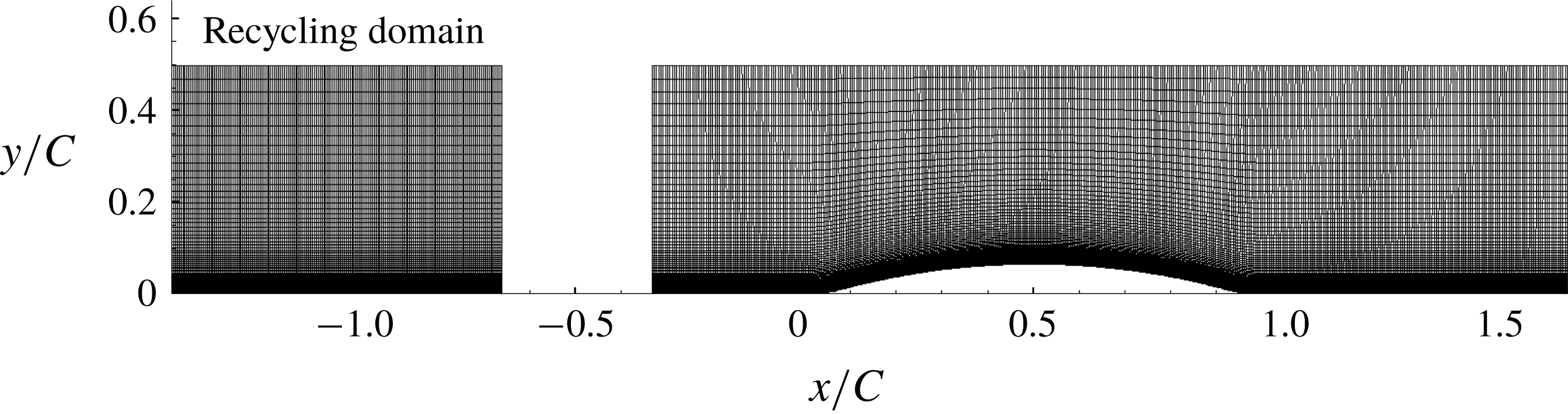
Mesh used for the LES simulation, shown for the h20 reference bump. Note the disconnected recycling domain for generating the inlet flow ( $C=0.305$ m).

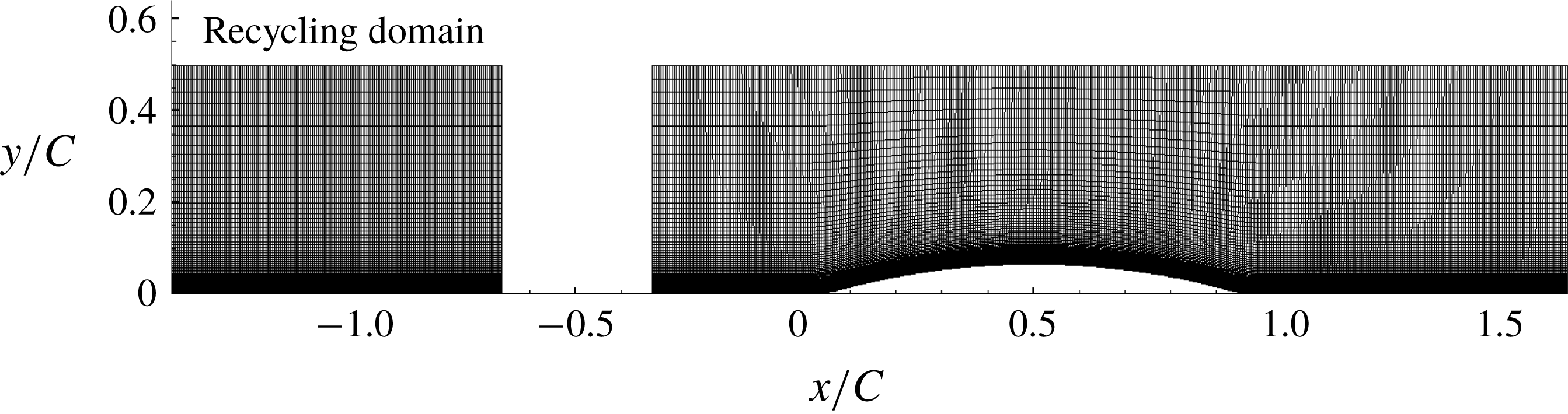
For the present study, the circular arc geometry of Webster, DeGraaff & Eaton (Reference Webster, Degraaff and Eaton1996) is adopted – see figure 1. The Webster et al. (Reference Webster, Degraaff and Eaton1996) data have been seen as a resource for testing turbulence models, and the present simulations have that as a motivation, too. The directly measured data are mean flow and Reynolds stresses. But, the best that can be done with such data is to compute with turbulence models, and compare. It would be valuable to go beyond that. This is the aim of modern, data-driven modelling. One would like to have data on turbulence model variables, such as $\unicode[STIX]{x1D708}_{T},~k,~\unicode[STIX]{x1D714}$ , as well. However, such quantities are not measurable, physical variables. They are defined by their role in a closure model, and cannot be measured directly. Even the variable $k$ , which is named ‘turbulent kinetic energy’, does not behave as the measurable turbulent kinetic energy. An innovative method to extract turbulence variables has been developed by Duraisamy, Zhang & Singh (Reference Duraisamy, Zhang and Singh2015) and Parish & Duraisamy (Reference Parish and Duraisamy2016). Turbulence variables are obtained by solving an optimization problem. Data on the variables of the $k$ – $\unicode[STIX]{x1D714}$ model, obtained by this method, will be presented in § 4. The prospect of improving turbulence models with those extracted data, and machine learning methods, is discussed in Singh et al. (Reference Singh, Matai, Mishra, Duraisamy and Durbin2017) and Matai & Durbin (Reference Matai and Durbin2019). To that end, a parametric series of datasets is helpful for training and testing.

The effects of pressure gradients, with and without surface curvature, have been studied previously by experiments and numerical simulations. These have explored various aspects of pressure gradient flows, such as disequilibrium, relaminarization and separation. Blackwelder & Kovasznay (Reference Blackwelder and Kovasznay1972) reported that a strong favourable pressure gradient resulted in the disappearance of the law of the wall and caused a decrease in the intermittency within the boundary layer. A numerical and experimental study by Spalart & Watmuff (Reference Spalart and Watmuff1993) of turbulent boundary layers with pressure gradients revealed that the buffer layer and lower end of the log layer shift up in FPG and down in APG. Bandyopadhyay & Ahmed (Reference Bandyopadhyay and Ahmed1993) also noticed a departure from the log law. Alving, Smits & Watmuff (Reference Alving, Smits and Watmuff1990) reported a slow recovery of the skin friction and Reynolds stresses after removal of a pressure gradient. The slow recovery is confirmed herein, but the profiles over the bump cannot be characterized by log-layer shifts; rather, the log layer ceases exist.

Disruption of the log law and substantial disequilibrium occur with relatively low bumps; the reference bump height in the present study is two-thirds of the inlet 99 % boundary layer thickness. Strong disequilibrium, in a simple geometry, adds a fundamental value to the present simulations.

2 Simulation overview

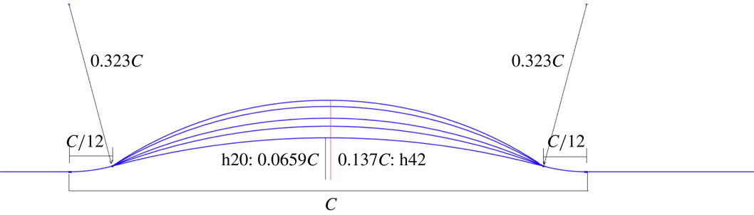
The geometry of Webster et al. (Reference Webster, Degraaff and Eaton1996) is shown in figure 1. It is a circular arc of length $L=254~\text{mm}$ and $h=20.1~\text{mm}$ . Convex fillets are added before and after the bump to create a total length of $C=305~\text{mm}$ . In § 3.2 this basic geometry will be extended by increasing $h$ , with other dimensions unchanged. The series is parametrized by $h/C$ , starting with $h/C=20/305$ , and increasing up to $42/305$ . The flow has separated by that value. The baseline geometry was previously simulated at a lower Reynolds number by Wu & Squires (Reference Wu and Squires1998), who were able to reproduce the experimental measurements via LES.

At present, the flow was simulated by wall-resolved LES in the finite volume code OpenFOAM (Weller et al. Reference Weller, Tabor, Jasak and Fureby1998). OpenFOAM uses a collocated grid arrangement with support for unstructured grids. The simulations were carried out with the unsteady and incompressible flow solver ‘pisoFoam’. The second-order, backward, implicit time advancement scheme was selected. Gauss-linear discretization was used for gradient and divergence terms, where ‘linear’ stands for a central differencing, second-order-accurate scheme to interpolate values from cell centres to face centres, and ‘Gauss’ specifies Gaussian integration. Laplacians were also discretized with the Gauss scheme and surface-normal gradients were computed with the corrected scheme, which is also second-order-accurate. The pressure and momentum equations were solved by preconditioned (bi)conjugate gradient. Diagonal incomplete-Cholesky factorization (pressure equation) and incomplete-LU factorization (momentum equation) was used for preconditioning. The PISO algorithm solves the pressure and momentum equation correctors two times in each step. Subgrid stresses were represented by the dynamic Smagorinsky model.

A time-dependent, turbulent inflow was generated by a separate, concurrent flat-plate boundary layer simulation as can be seen in figure 1. The disconnected, upstream domain recycles and rescales the flow (Arolla Reference Arolla2016) to generate fully developed inflow to the downstream domain. The inlet momentum thickness was $\unicode[STIX]{x1D6E9}=3.6~\text{mm}$ ; hence, for the baseline case $\unicode[STIX]{x1D6E9}/h=0.18$ and $\unicode[STIX]{x1D6FF}_{99}/h=1.5$ . This same thickness was used for the higher bumps. The time step, $\text{d}t=0.009\unicode[STIX]{x1D6E9}/U_{ref}$ , ensured a maximum Courant–Friedrichs–Lewy (CFL) number ${<}0.7$ , where $U_{ref}$ is the inlet free-stream velocity.

The inlet to the bump is located at $x/C=-1/3$ with an inlet Reynolds number of 2500 based on inlet free-stream velocity and momentum thickness ( $=C/82$ ). The bump starts at $x/C=0$ and ends at $x/C=1$ and the width of the domain is $0.22C$ . The top boundary condition is zero normal-gradient for the velocity and pressure, and the outlet condition is zero normal gradient for the velocity, and zero pressure.

2.1 Verification

Figure 2.

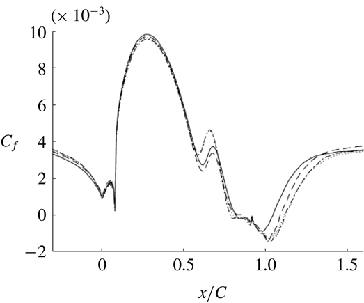
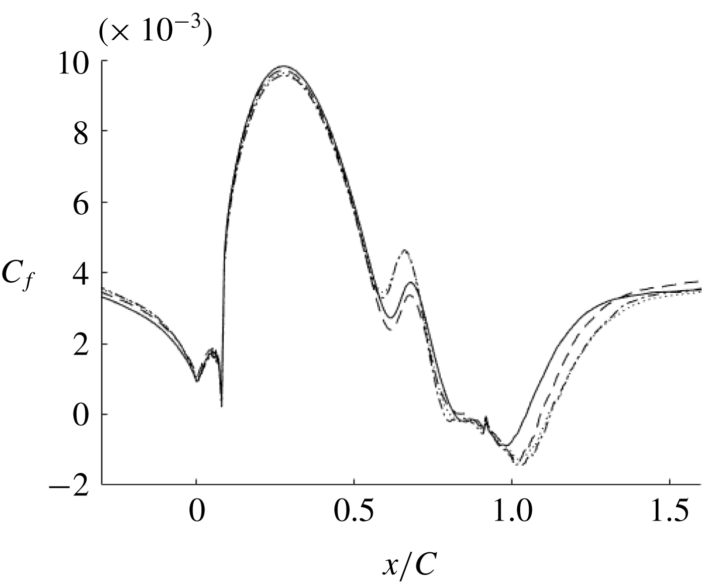
Grid convergence for highest bump (h42), LES: ——, mesh 1; - - - -, mesh 2; $\cdots \cdots$ , mesh 3; — - —, mesh 4.

Table 1.

Grid characteristics of the bump simulation at $Re_{\unicode[STIX]{x1D703}}=2500$ .

As the highest bump has the largest separation and requires the finest grid, a sensitivity study is shown for this bump. This same resolution was used for all the bumps. Table 1 gives the grid characteristics for the different resolutions that were tested and figure 2 shows the skin friction for these meshes. The grid spacing is in plus units, using the friction velocity at the inlet. LES is inherently grid-dependent. Hence, the grid dependence in figure 2 can be regarded as a measure of experimental accuracy. The accuracy is very good, and even better for the lower bumps; indeed, the reference bump is virtually grid-independent.

It was observed that resolution in the spanwise and streamwise directions was more important for accuracy than was the wall-normal direction. The streamwise resolution was most important in the APG region. As seen in figure 2, the upstream region is virtually grid-independent. Hence, streamwise refinements were made after the crest of the bump; before the crest, all meshes have the same streamwise resolution (Matai Reference Matai2018).

Mesh 3 and mesh 4 had identical skin friction and velocity profiles, indicating that mesh 3 had sufficient resolution and, thus, was chosen for all the simulations.

The ratio of the subgrid viscosity to molecular viscosity is a standard metric for LES resolution. The ratio was less than 2 over almost all of the domain, which indicates very good LES resolution (Durbin & Reif Reference Durbin and Reif2011).

Figure 7, below, shows that the domain width is sufficient to capture several high- and low-speed streaks, indicating that the domain width was sufficient in the $z$ -direction. Further verification studies are reported in Matai (Reference Matai2018).

2.2 Validation

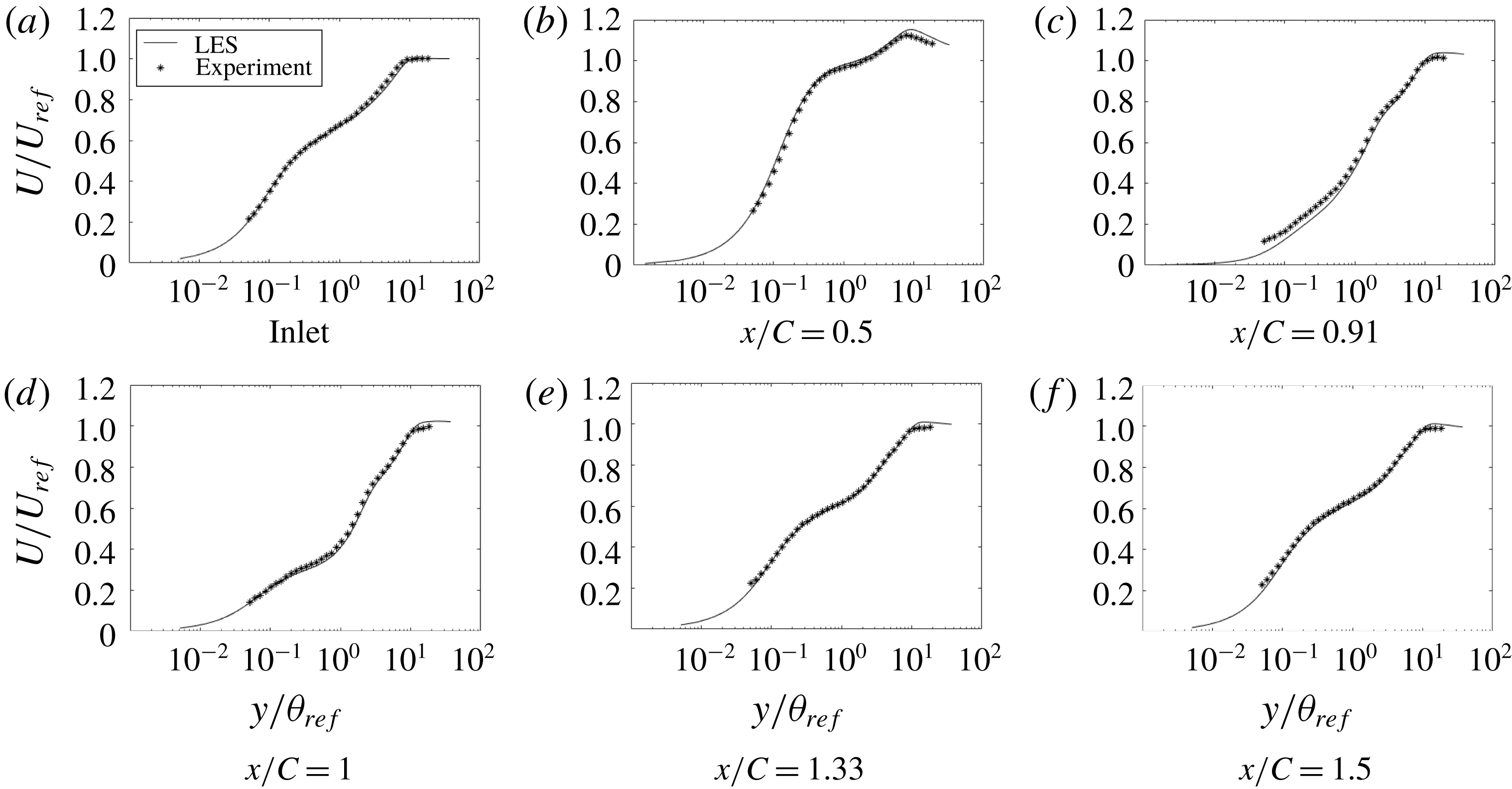
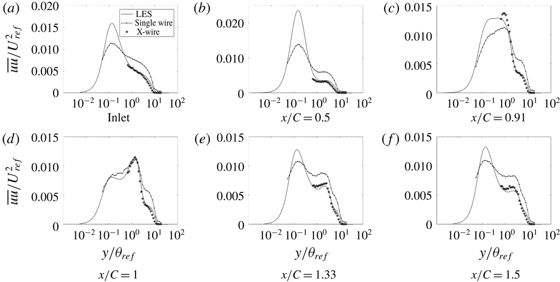
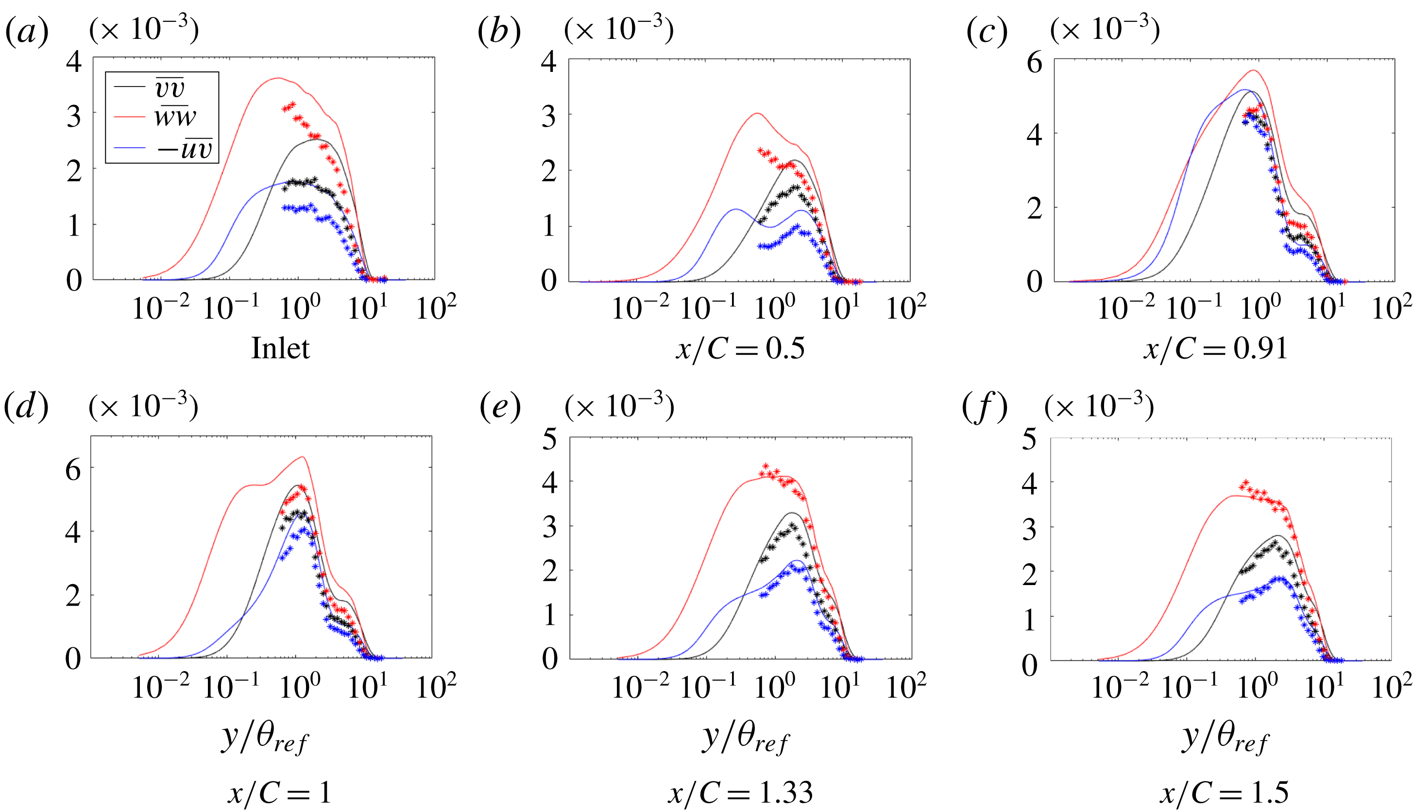
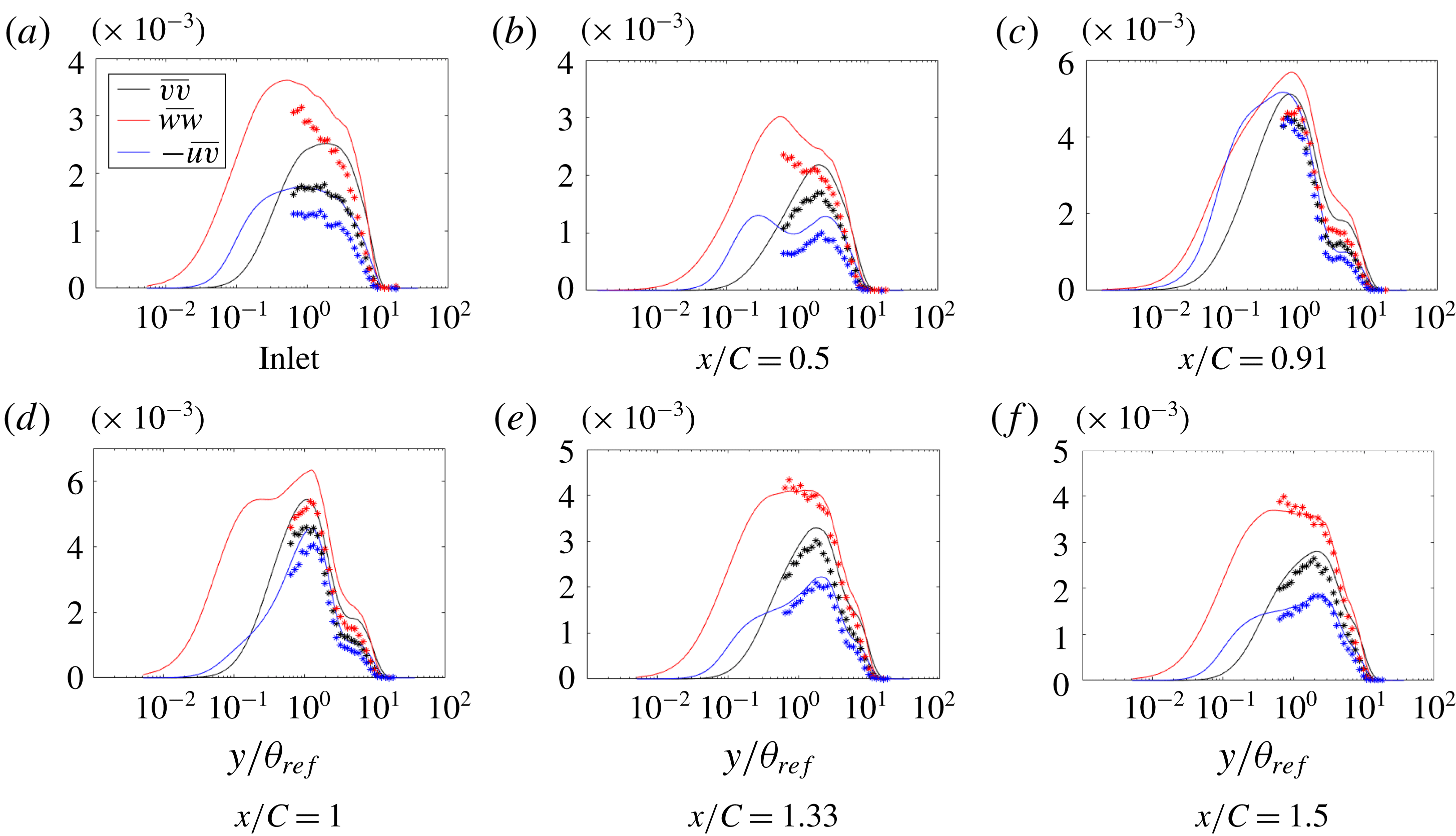
Time- and span-averaged velocity profiles were compared with experimental data (Webster et al. Reference Webster, Degraaff and Eaton1996). Those data are for the lowest bump, only. The published data are at $Re_{\unicode[STIX]{x1D703}}=4000$ , but unpublished data are available for the present $Re_{\unicode[STIX]{x1D703}}=2500$ . Those were used in figure 3. Velocity is scaled on the inlet free-stream velocity, and the inlet momentum thickness is the length scale. Components of Reynolds stresses, $\overline{uu}$ (figure 4), $\overline{vv}$ , $\overline{ww}$ and $\overline{uv}$ (figure 5), were also compared.

Figure 3.

Time- and span-averaged $x$ -velocity at various $x$ locations: ——, LES; $\ast$ , experiment.

The LES profiles of mean velocity in the $x$ -direction match extremely well with the experimental data. Over the bump, figure 3 shows large deviations from the log law; this will be seen clearly below in figure 13, where velocity is normalized by viscous units. The experimentalists noted the absence of a log layer, too, and used an oil drop method to infer skin friction.

Figure 4.

Time- and span-averaged $\overline{uu}$ at various $x$ locations: ——, LES; — - —, single wire; $\ast$ , X-wire.

The $\overline{uu}$ profiles, figure 4, match well with the X-wire experimental data, where they are available. However, the LES shows structure close to the wall that could not be measured by the X-wire. The experimenters measured some data with a single wire, but they are not quantitatively accurate. The single-wire data are included to show that the near-wall behaviour, seen in the LES, was also present in the laboratory experiment. The $\overline{uu}$ peak is an order of magnitude larger than the other diagonal components of the Reynolds stress tensor. The peaks of $\overline{uu}$ at $y_{+}\sim 11$ are at the position of highest production in a zero pressure gradient (ZPG) flat-plate boundary layer ( $y_{+}=11$ ).

The $\overline{vv}$ and $\overline{ww}$ data are slightly overpredicted by LES. This is similar to what Wu & Squires (Reference Wu and Squires1998) observed. The $\overline{uv}$ component (figure 5), also, is slightly overpredicted by LES.

Figure 5.

Time- and span-averaged $\overline{vv}$ , $\overline{ww}$ and $-\overline{uv}$ at various $x$ locations normalized by $U_{ref}^{2}$ : ——, LES; $\ast$ , experiment.

Figure 6.

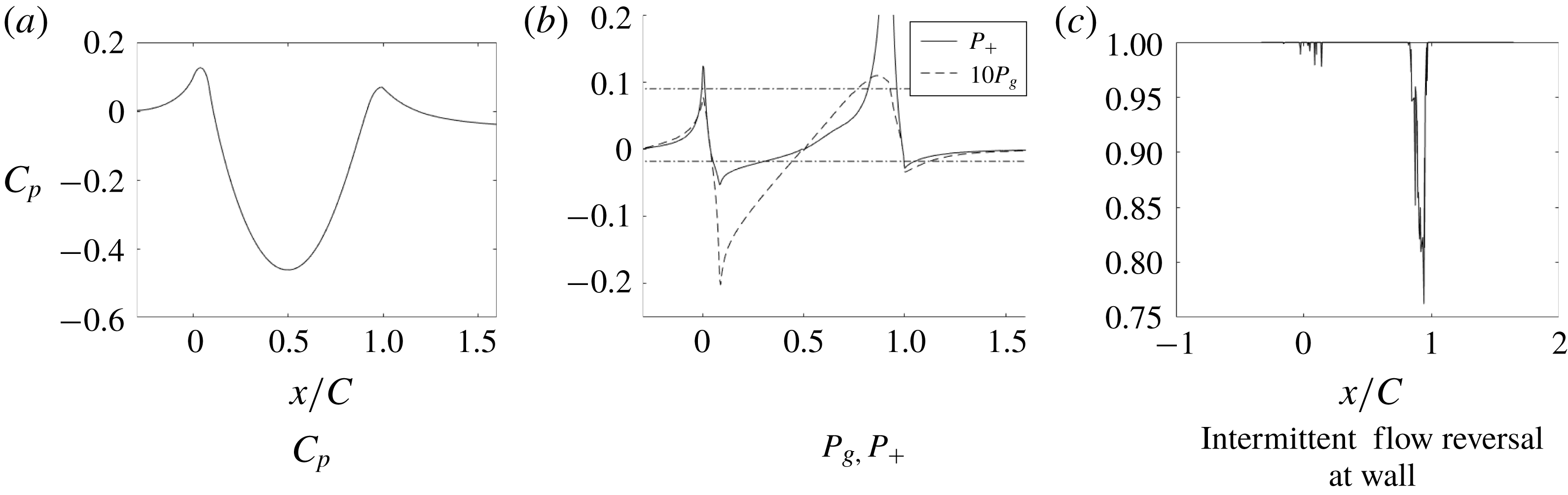
Pressure coefficient, pressure gradient parameters and intermittent flow reversal at the wall.

Figure 7.

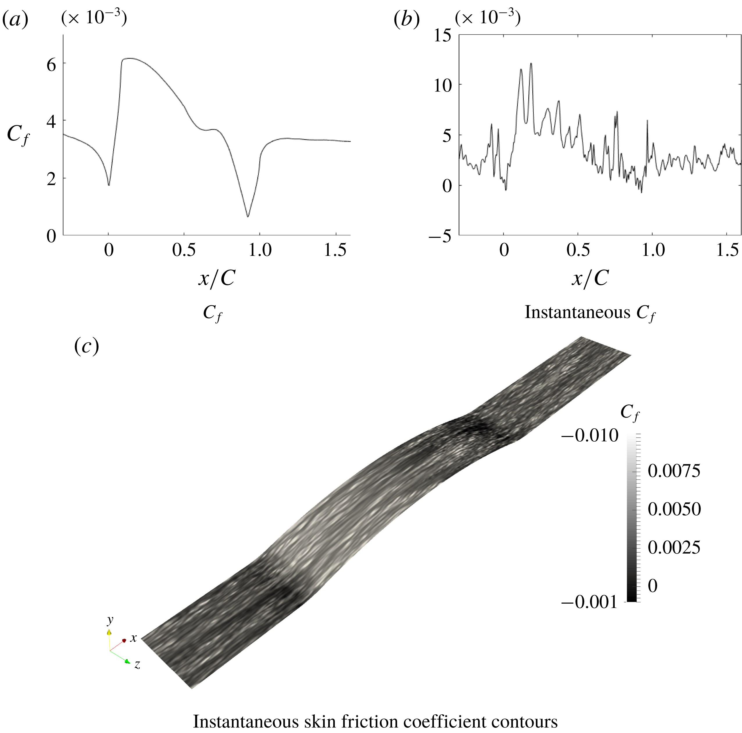
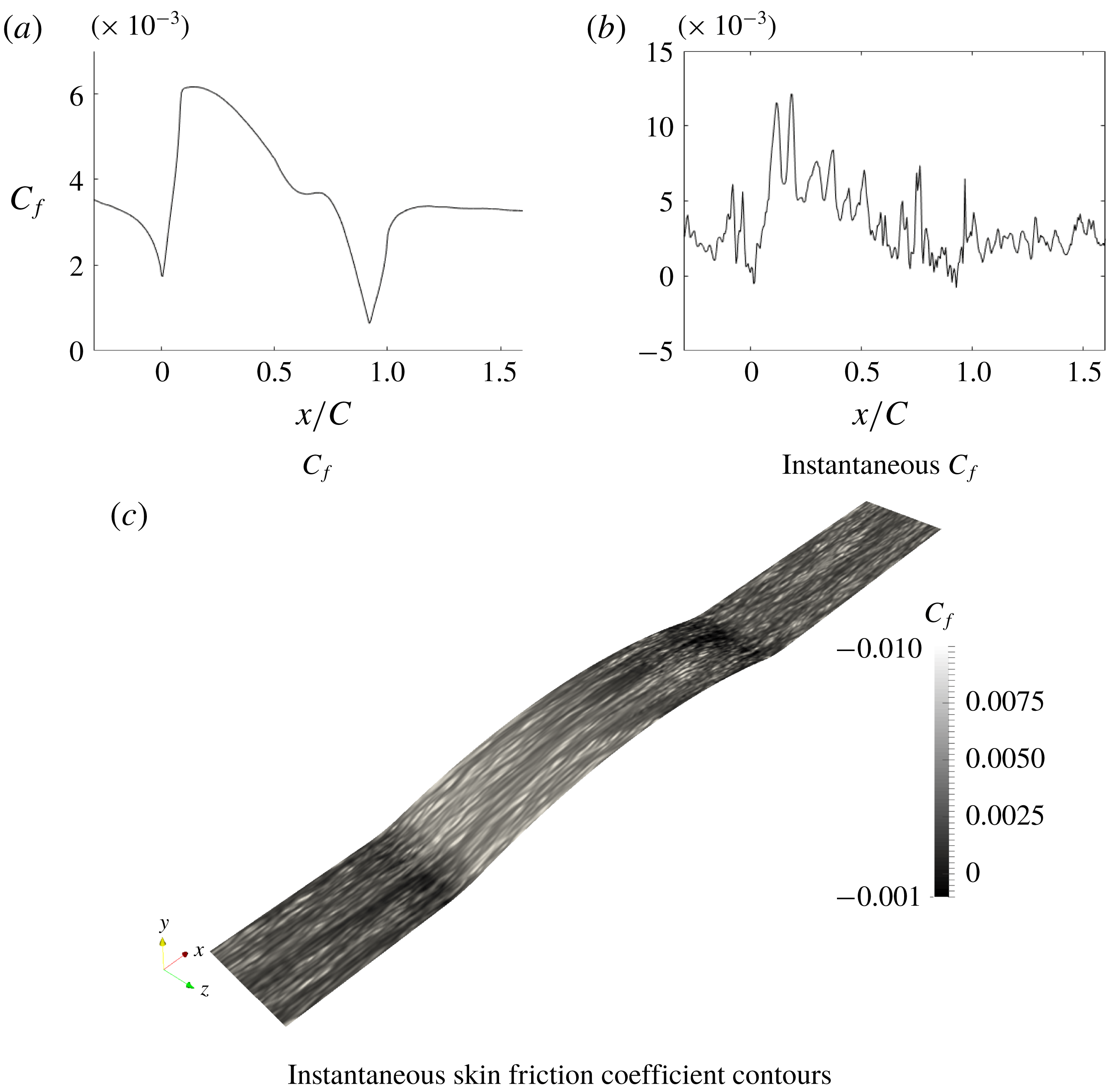
Skin friction coefficient.

3 Flow analysis

3.1 Base case

The surface static pressure coefficient and non-dimensionalized gradient of pressure are plotted in figure 6. The pressure gradient is adverse as the flow approaches the bump and then becomes favourable until the crest of the bump. It then becomes adverse and drops to being favourable in the recovery region of the flow.

The effect of the sudden change in pressure gradient at the start and end of the bump can be seen on the skin friction coefficient (figure 7); it too exhibits sudden increase and decrease at $x/C=0$ and $x/C=1$ . The skin friction coefficient shows a plateau from $x/C=0.6$ to 0.8. The plateau (observed in this case of $Re_{\unicode[STIX]{x1D703}}=2500$ ) was attributed by Wu & Squires (Reference Wu and Squires1998) to intermittent flow reversal at the wall; intermittent flow reversal is the percentage of time the skin friction is negative. At their $Re_{\unicode[STIX]{x1D703}}=1500$ , the streamwise locations of the $C_{f}$ plateau and the intermittent flow reversal coincide. This, however, is not the case at the current Reynolds number. Figure 6 shows that the intermittent flow reversal at the wall occurs at $x/C=0.8$ , which is after the plateau.

The non-dimensional pressure gradient parameters, defined as

(3.1a,b )

$$\begin{eqnarray}P_{g}=\frac{\text{d}\overline{p}_{w}}{\text{d}s}\frac{\unicode[STIX]{x1D703}_{ref}}{U_{ref}^{2}},\quad P^{+}=\frac{\text{d}\overline{p}_{w}}{\text{d}s}\frac{\unicode[STIX]{x1D708}}{\unicode[STIX]{x1D70F}_{w}^{3/2}},\end{eqnarray}$$

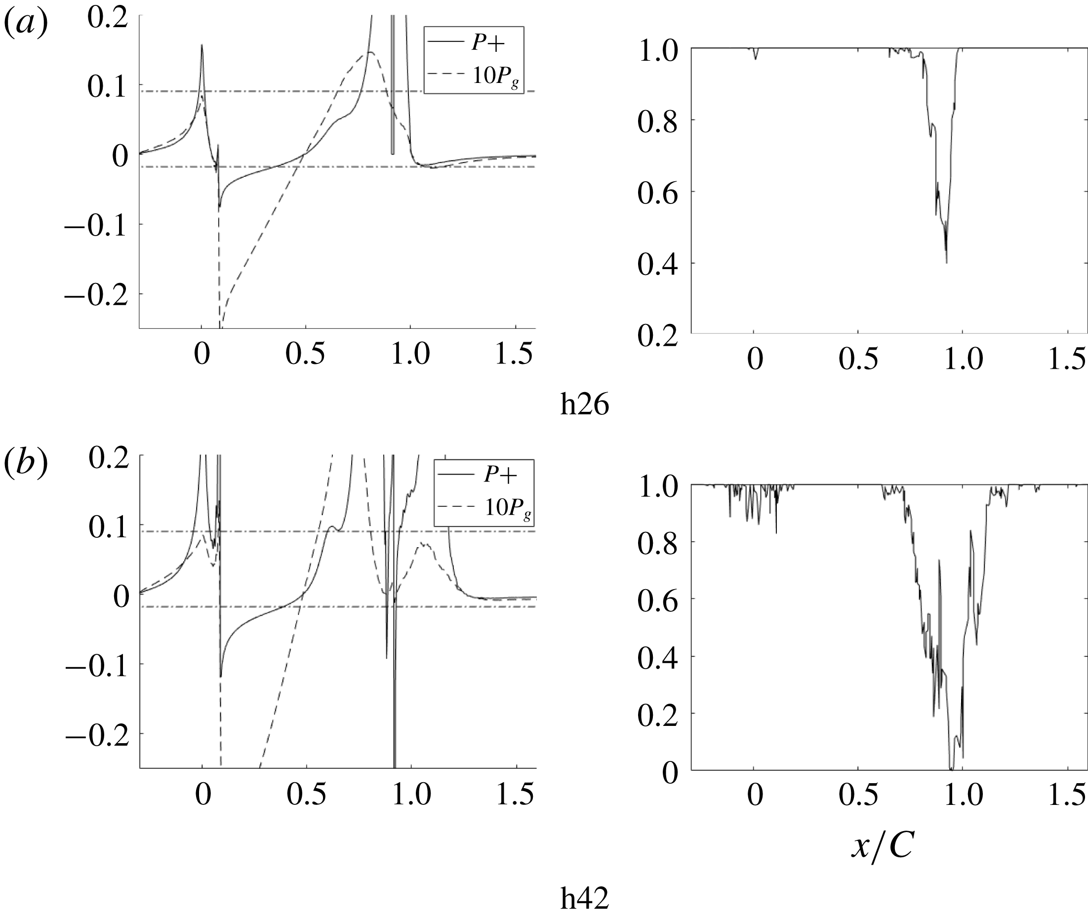
are shown in figure 6(b). There, $P^{+}=0.09$ , marked in the figure, was suggested by Patel (Reference Patel1965) as a criterion for the onset of separation; indeed, it correlates with the beginning of intermittent flow reversal at the wall. Patel (Reference Patel1965) suggested $P^{+}=-0.018$ , also marked in the figure, as a criterion for the onset of relaminarization. The pressure gradient parameter crosses this mark, briefly, just near the front of the bump, but is above it near the crest.

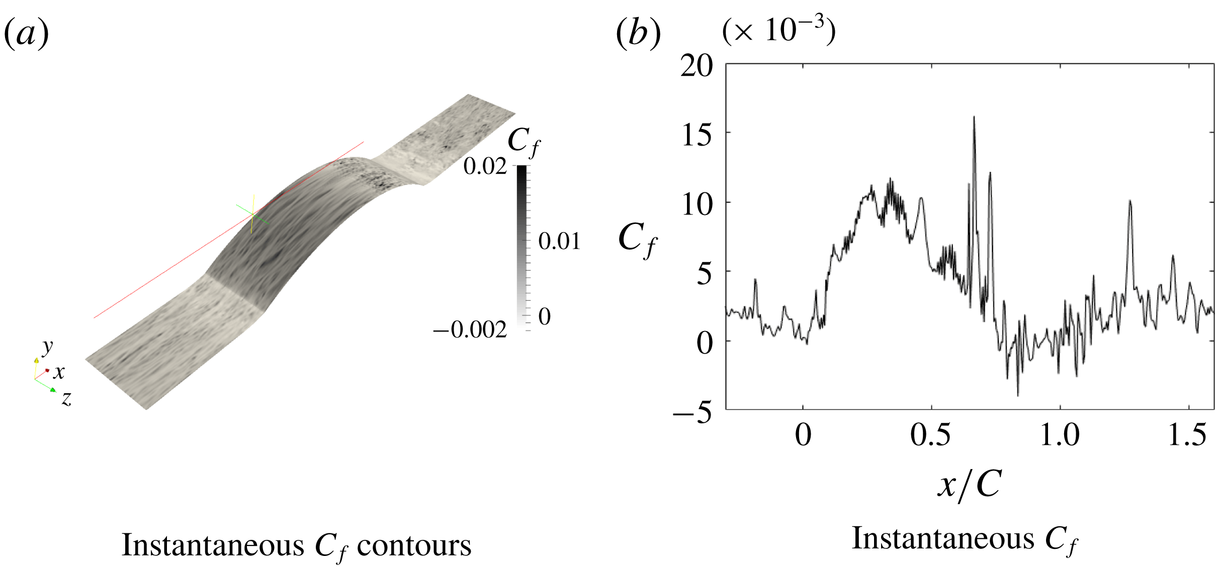
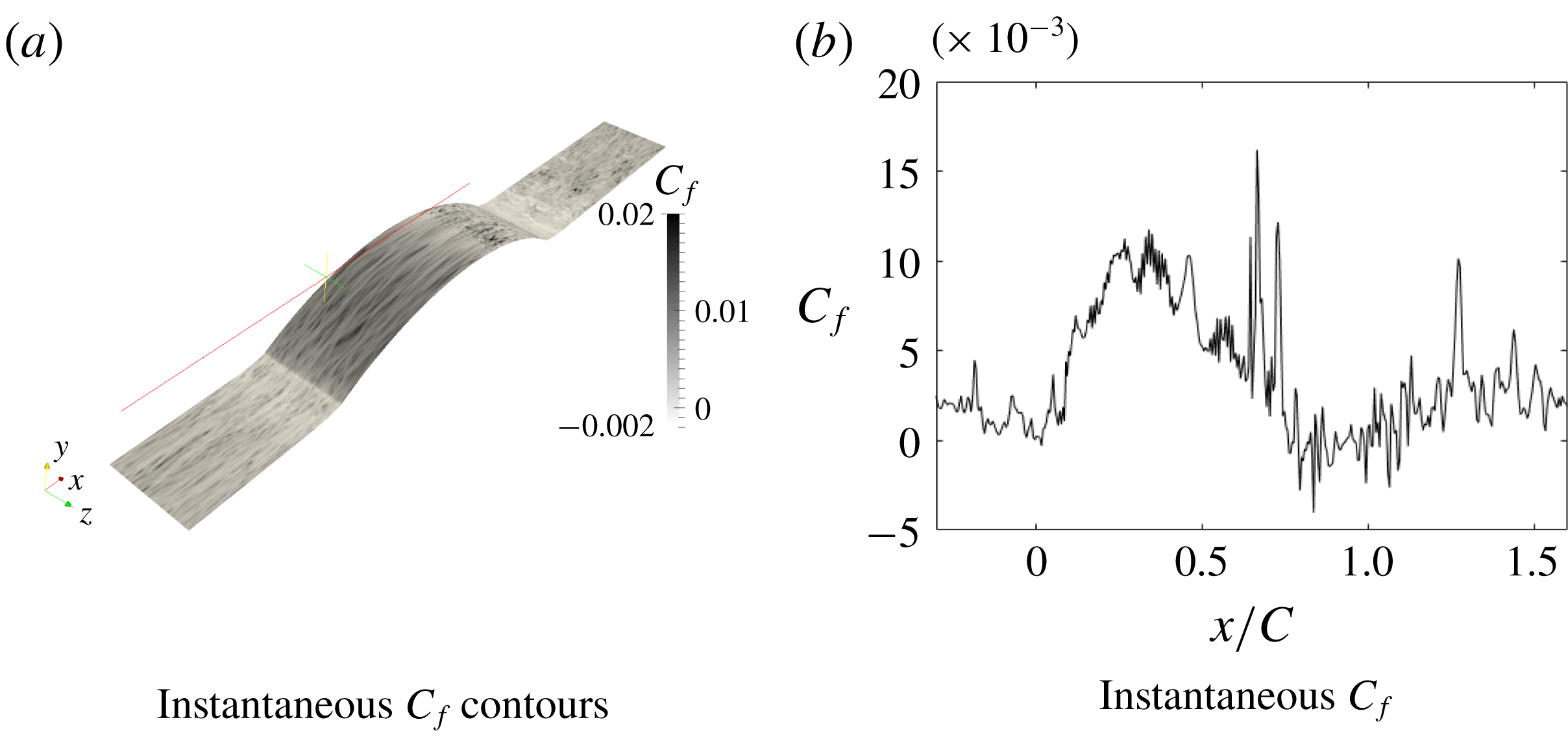
There has been speculation that the Webster et al. (Reference Webster, Degraaff and Eaton1996) bump relaminarized at the crest. That was partly because turbulence closure models did not capture the flattening of the $C_{f}$ curve, near the crest. However, even for the highest bump, we found this not to be the case. The instantaneous $C_{f}$ at the mid-span plane is plotted in figure 7 to illustrate that the flow does not become laminar. This and the instantaneous skin friction coefficient contours (figure 7) show turbulent fluctuations. In § 4 it will be seen that the flow can be predicted by a fully turbulent RANS computation.

3.2 Bump series

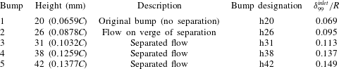
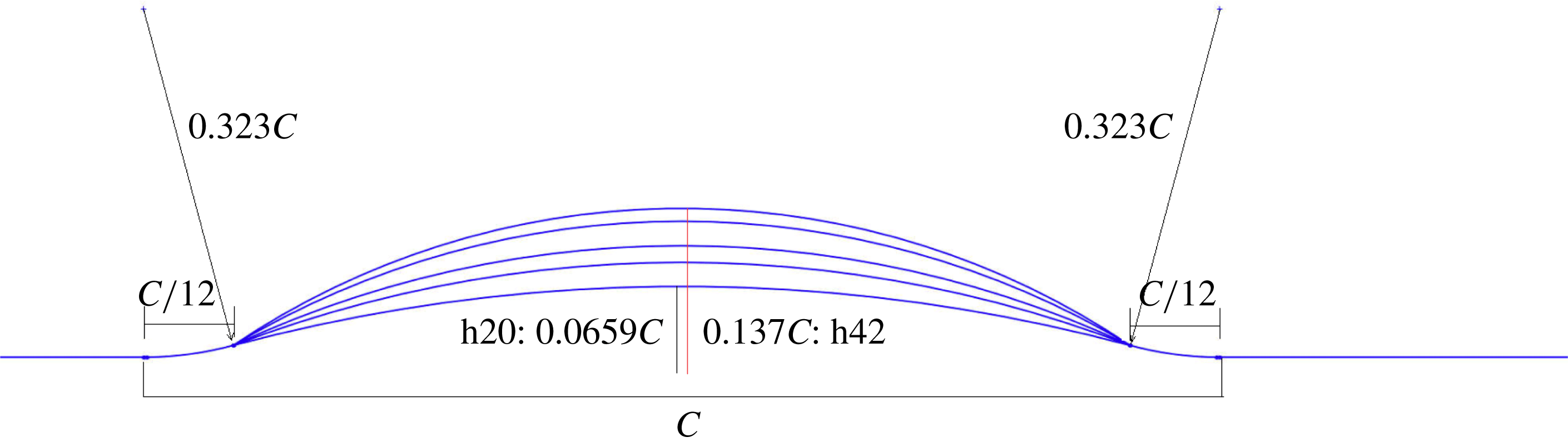
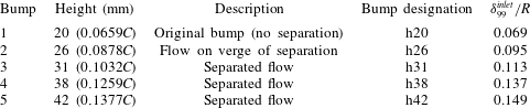
In order to study the progression towards separation, the flow over bumps of increasing height was simulated. The bump geometries are shown in figure 8. The set of bumps is summarized in table 2. The bumps were created by fitting a circular arc between three points: the end of the first convex fillet, the crest of the bump and the beginning of the last convex fillet.

Figure 8.

Bump geometries.

Table 2.

Summary of bumps.

Figure 9.

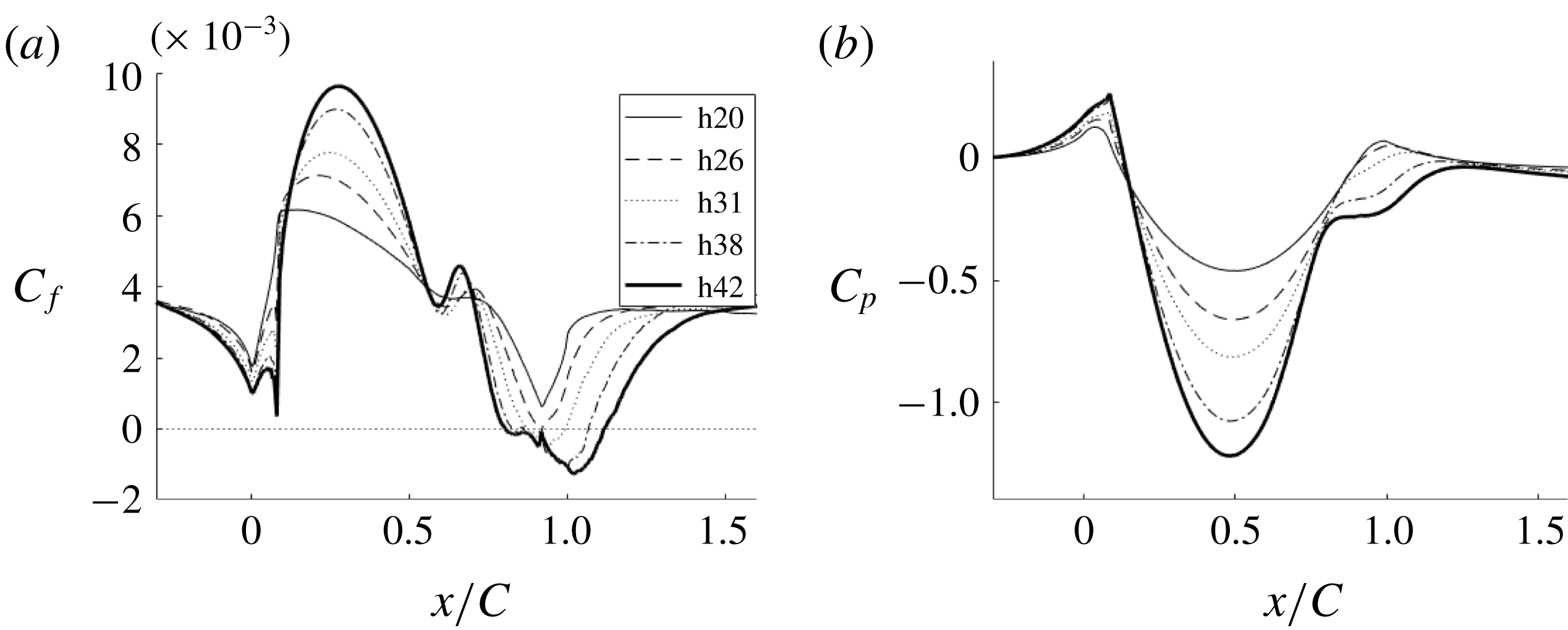
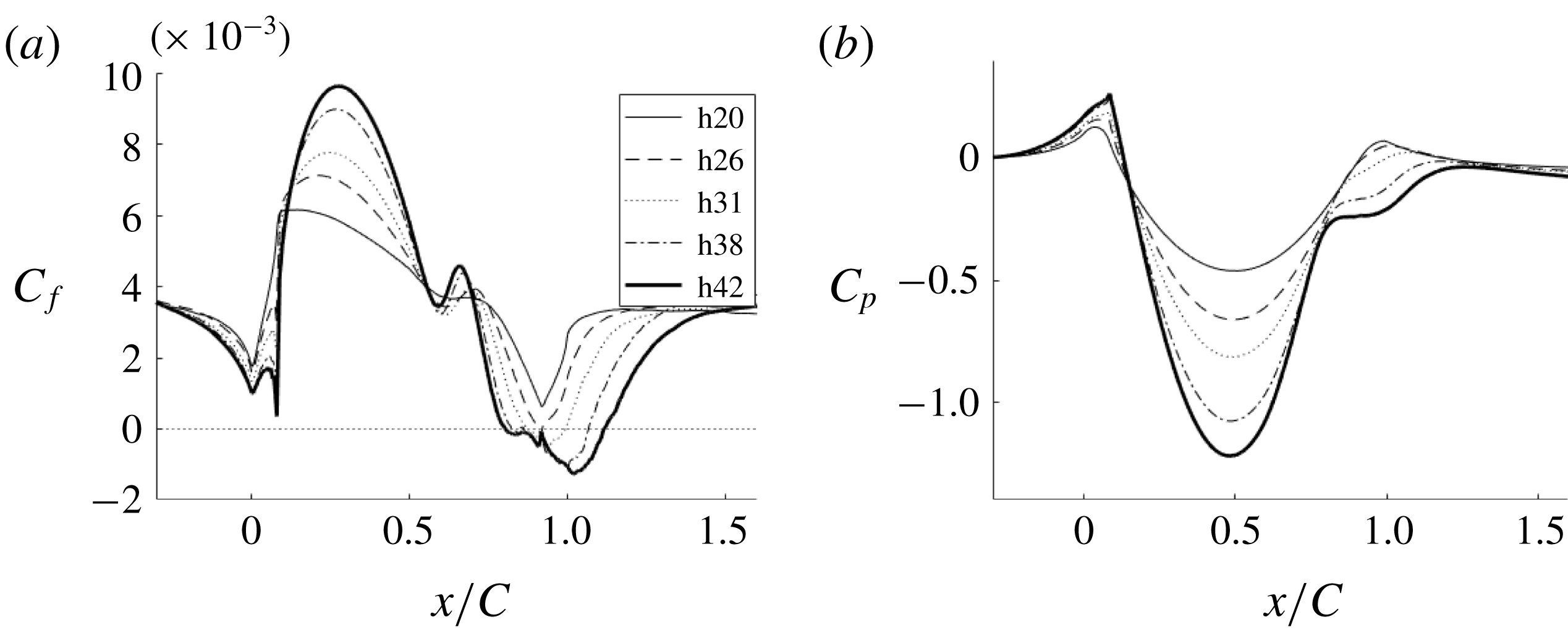
Comparison of skin friction coefficient and pressure for different bump crest heights.

Figure 10.

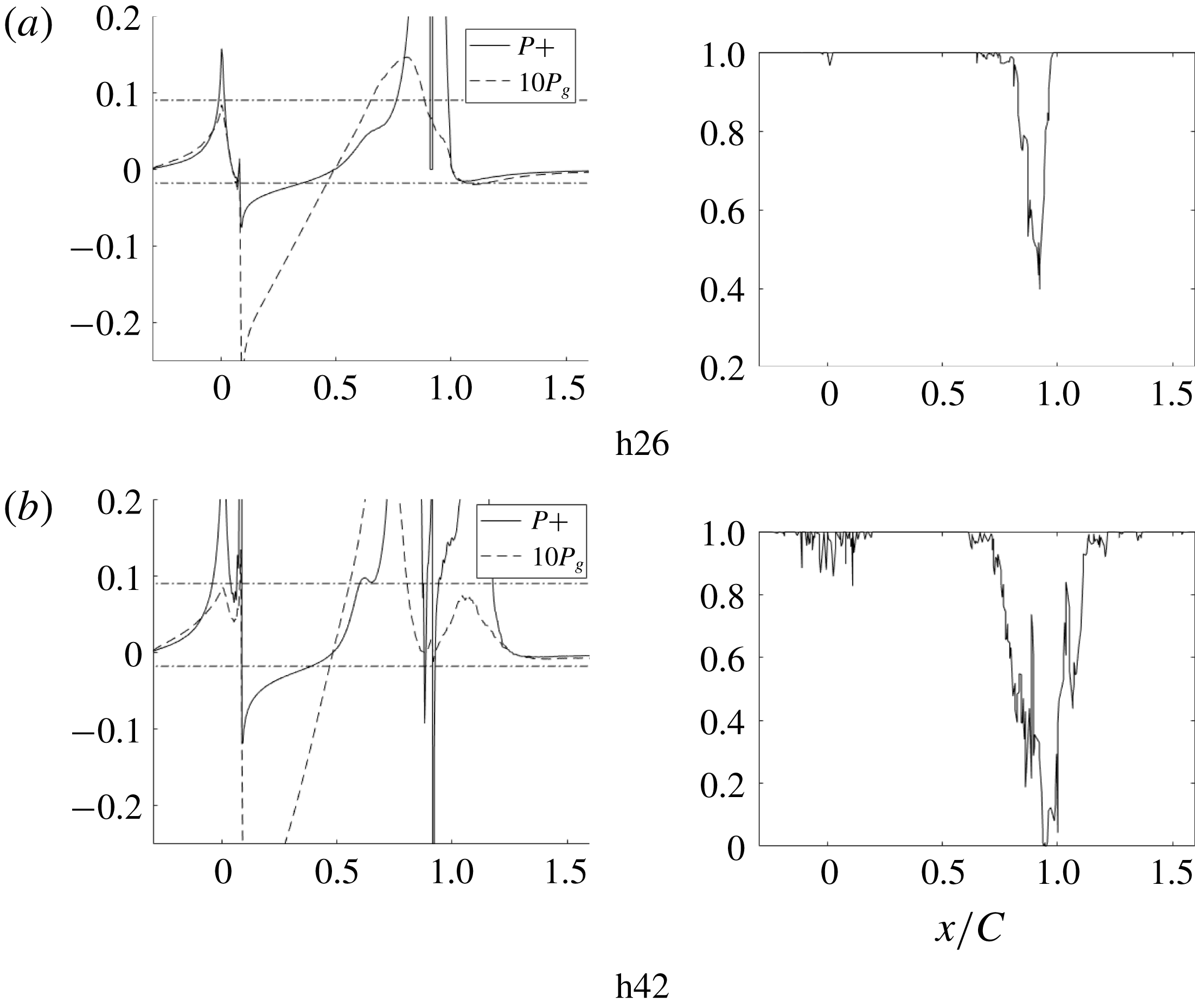
Pressure gradient parameters and intermittent flow reversal at the wall for bumps with different crest heights.

Figure 11.

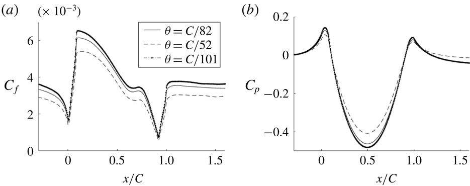
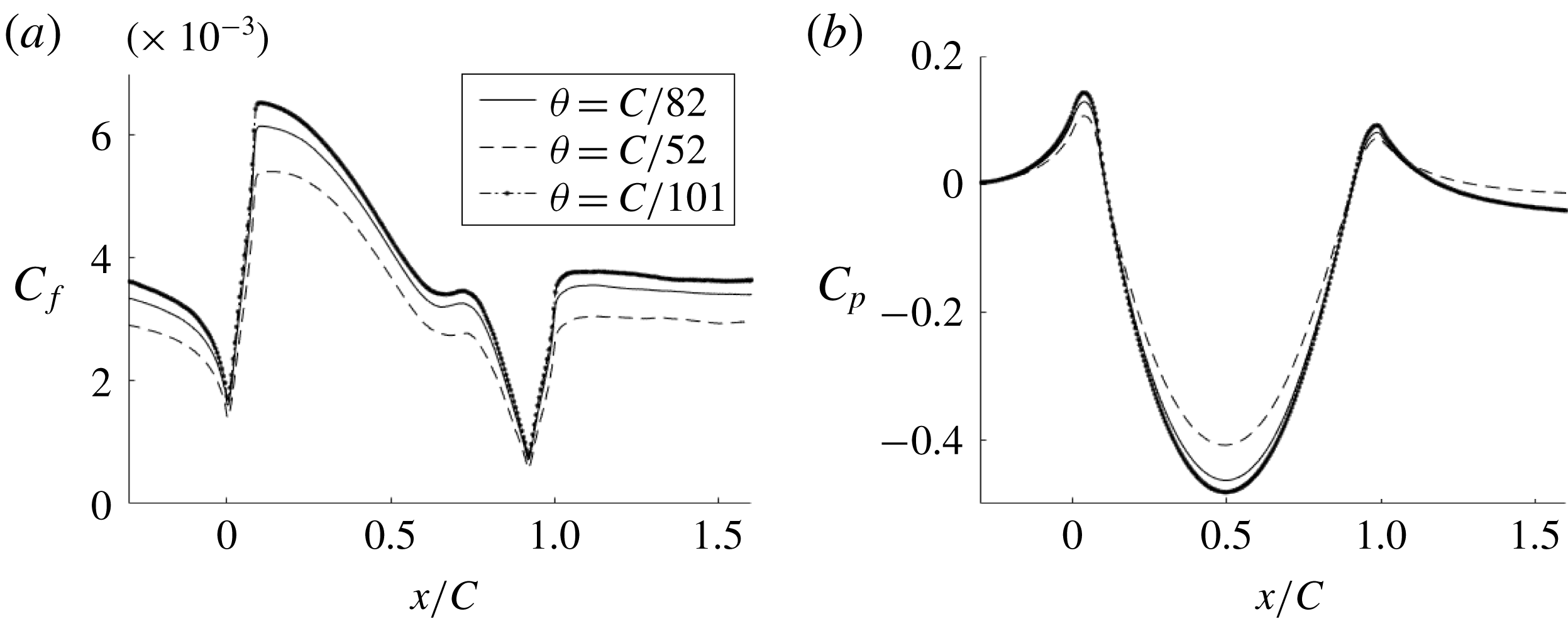
Comparison of skin friction coefficient and pressure for different inlet momentum thicknesses (h20).

Figure 12.

Instantaneous skin friction coefficient for h42.

Figure 13.

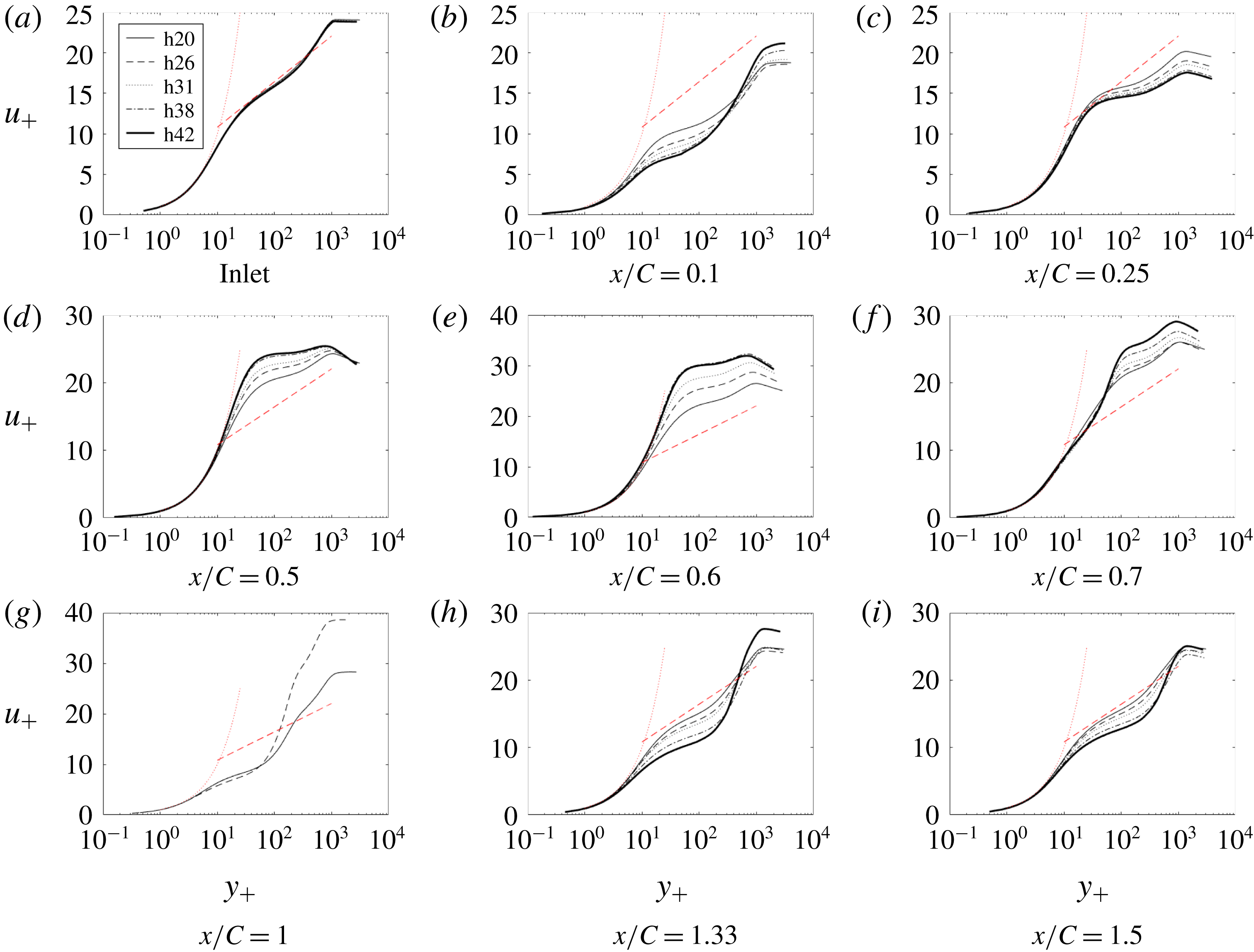
Time- and span-averaged $x$ -velocity at various $x$ locations: ——, h20; - - - -, h26; $\cdots \cdots$ , h31; — - —, h38; _______, h42.

Figure 14.

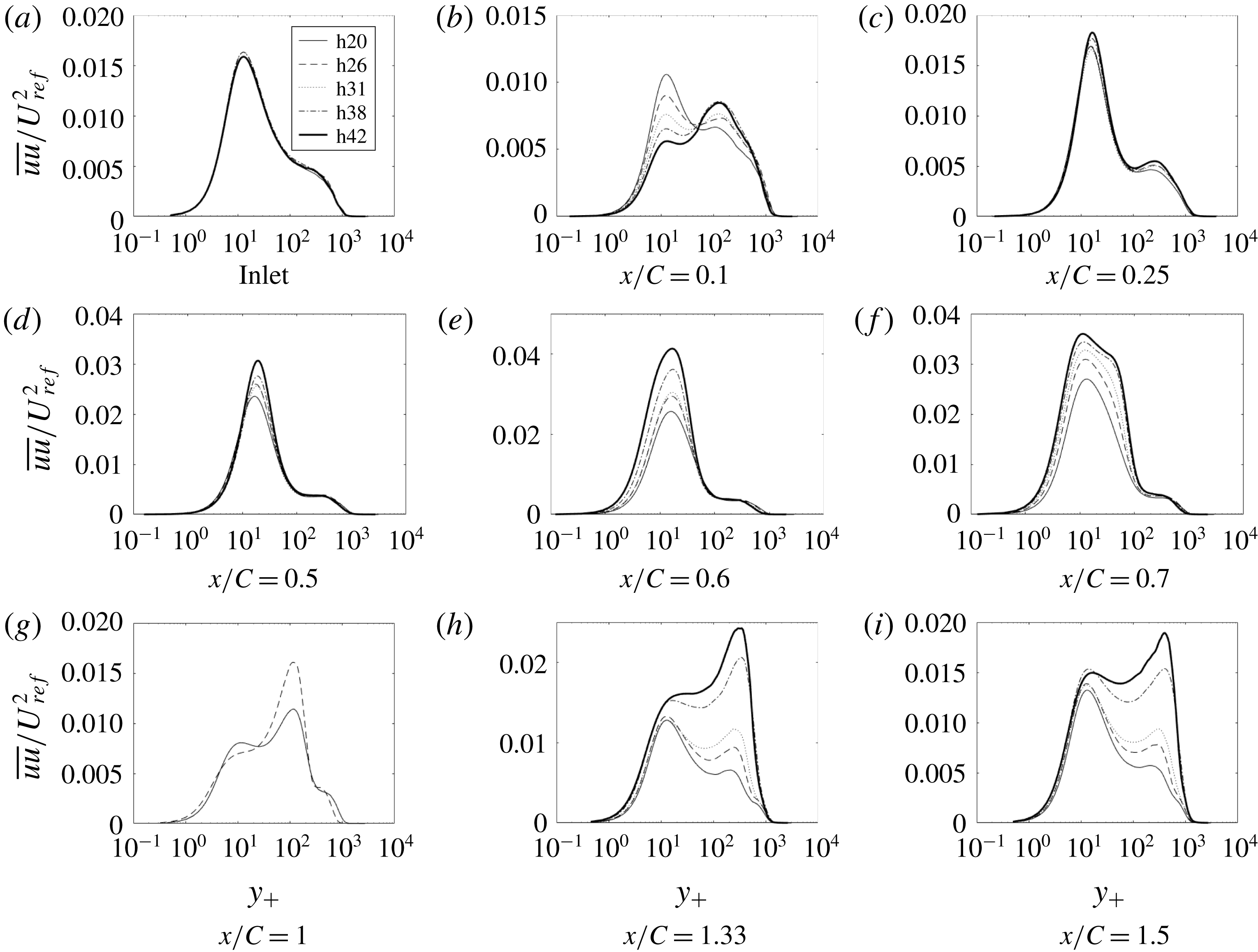
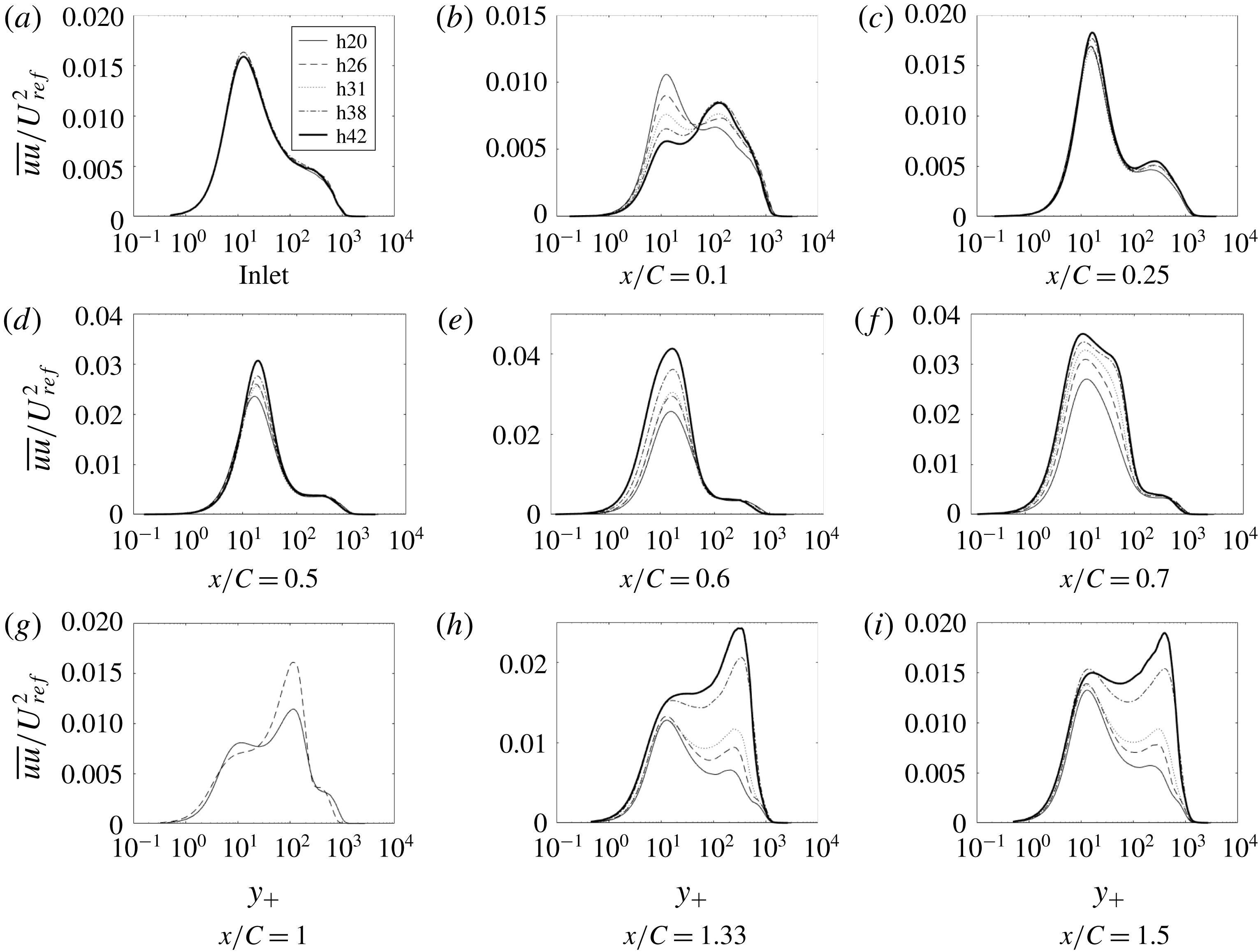
Time- and span-averaged $\overline{uu}$ at various $x$ locations: ——, h20; - - - -, h26; $\cdots \cdots$ , h31; — - —, h38; _______, h42.

Figure 15.

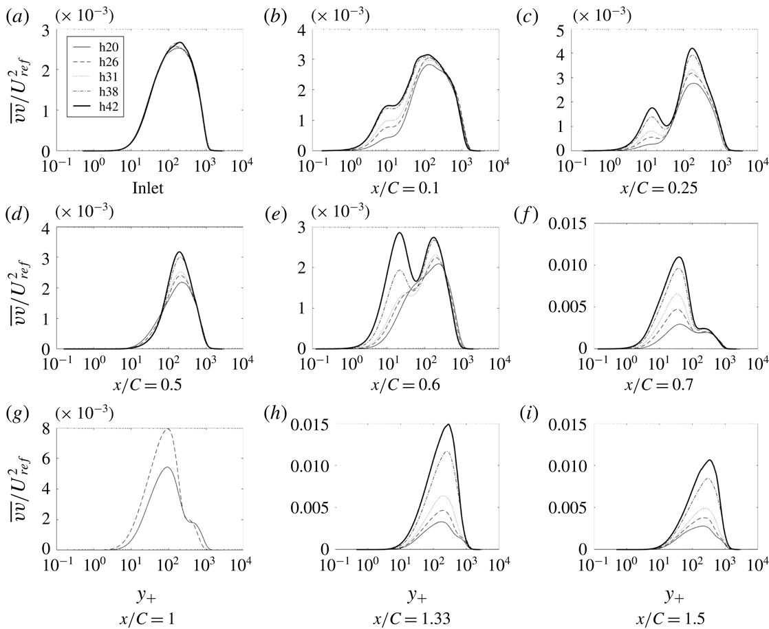
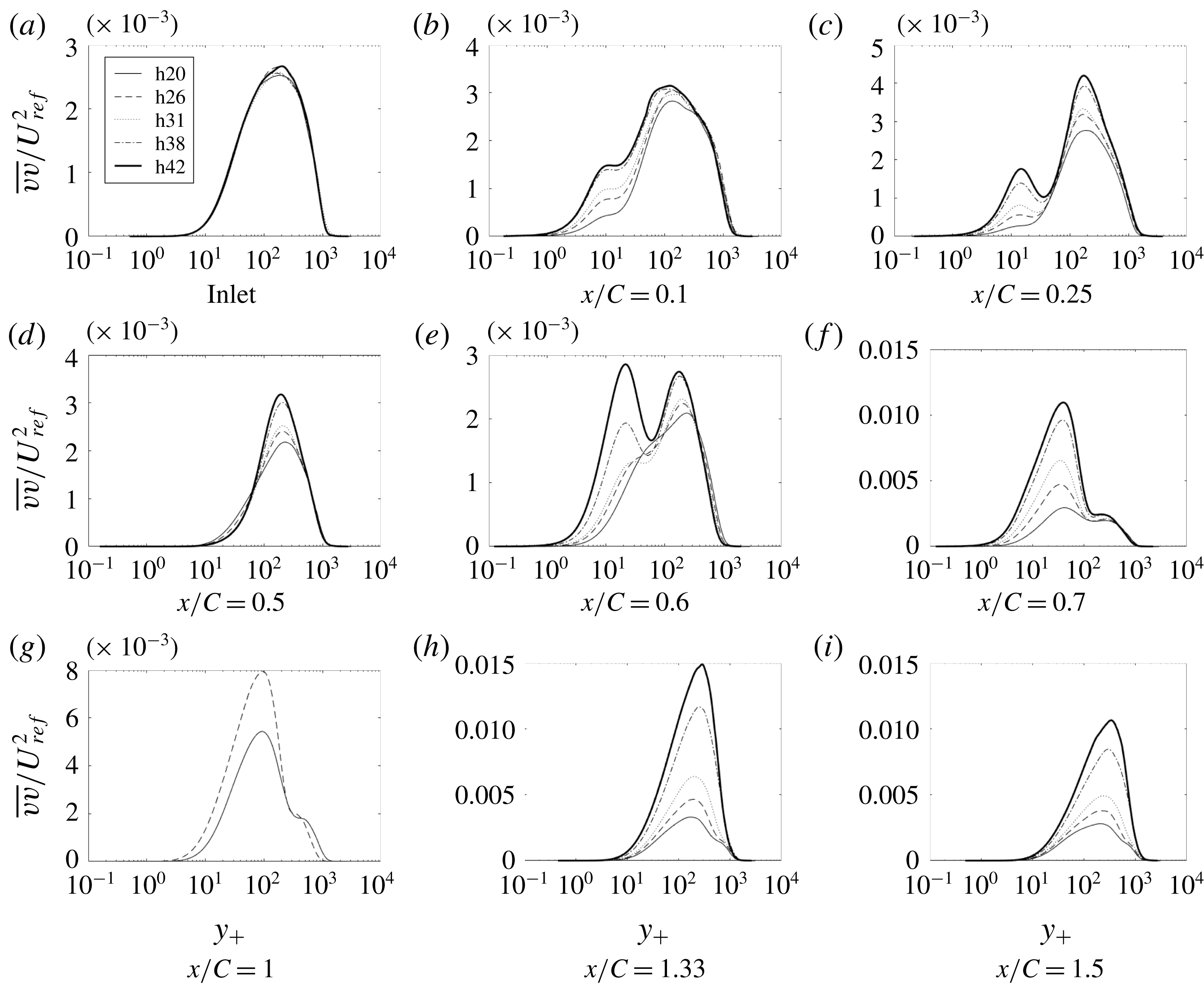
Time- and span-averaged $\overline{vv}$ at various $x$ locations: ——, h20; - - - -, h26; $\cdots \cdots$ , h31; — - —, h38; _______, h42.

Figure 16.

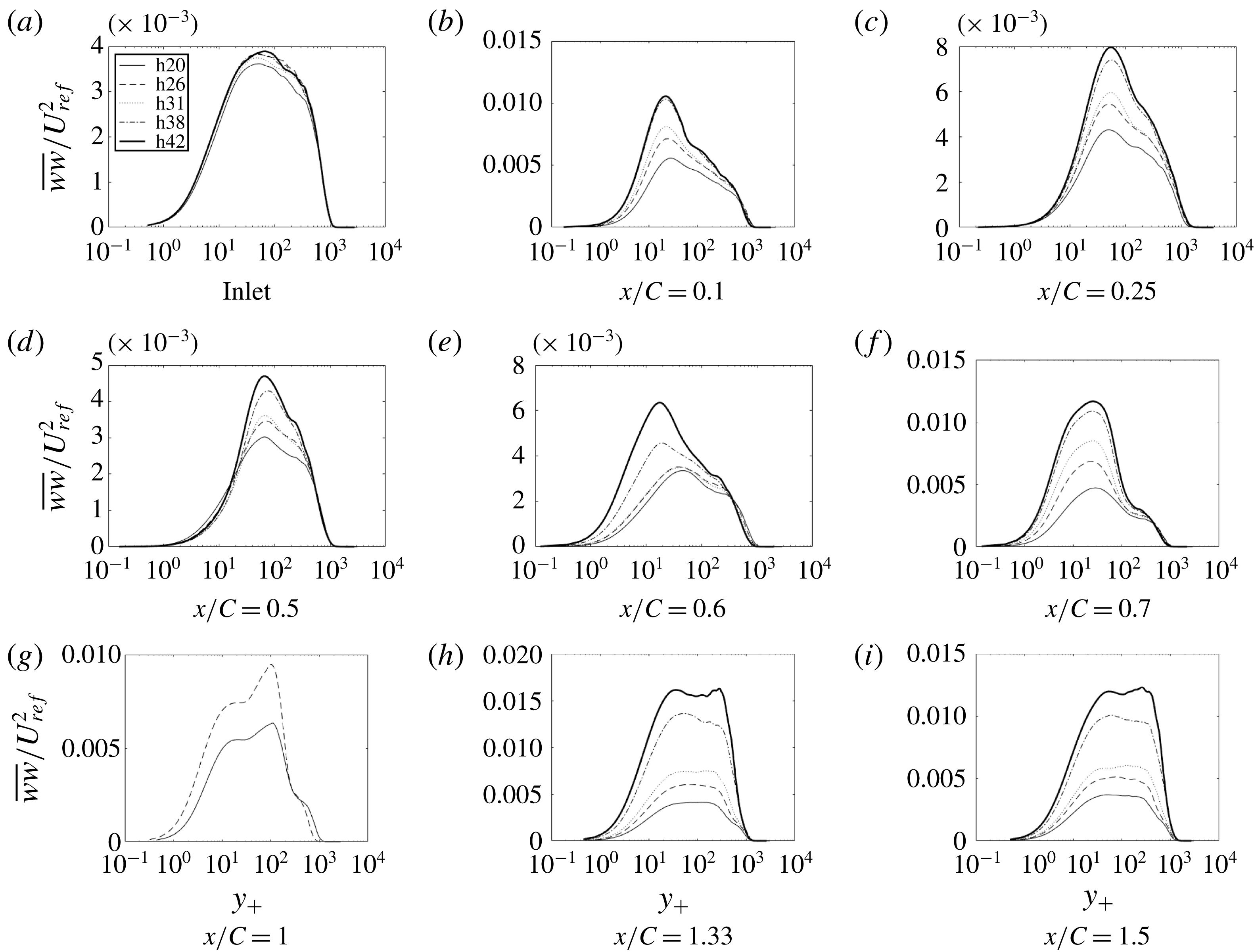
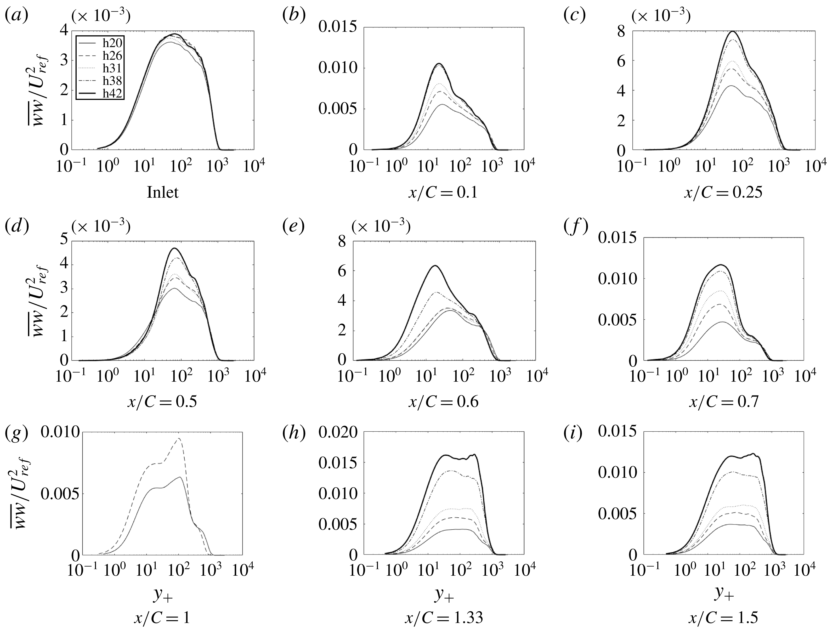
Time- and span-averaged $\overline{ww}$ at various $x$ locations: ——, h20; - - - -, h26; $\cdots \cdots$ , h31; — - —, h38; _______, h42.

Figure 17.

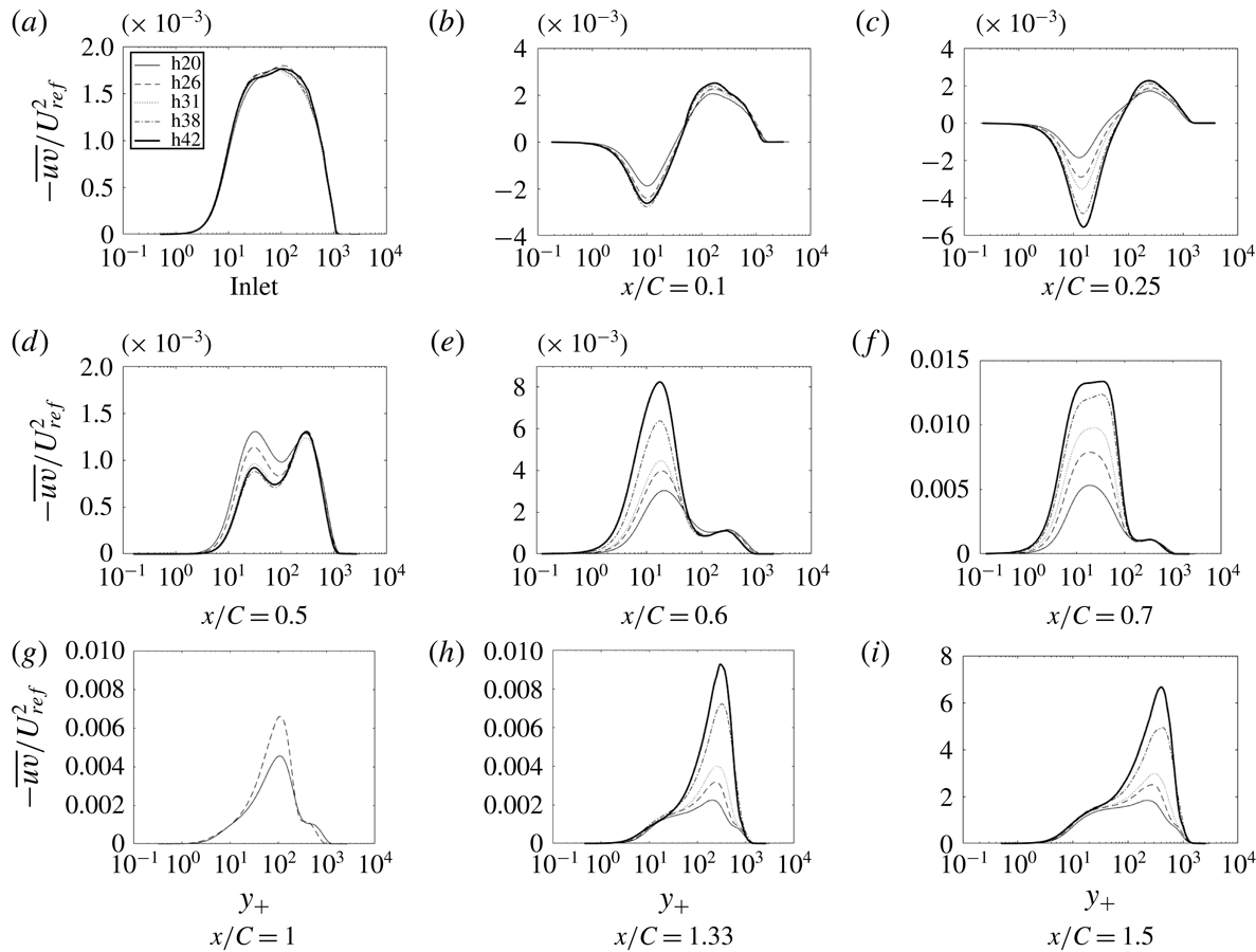
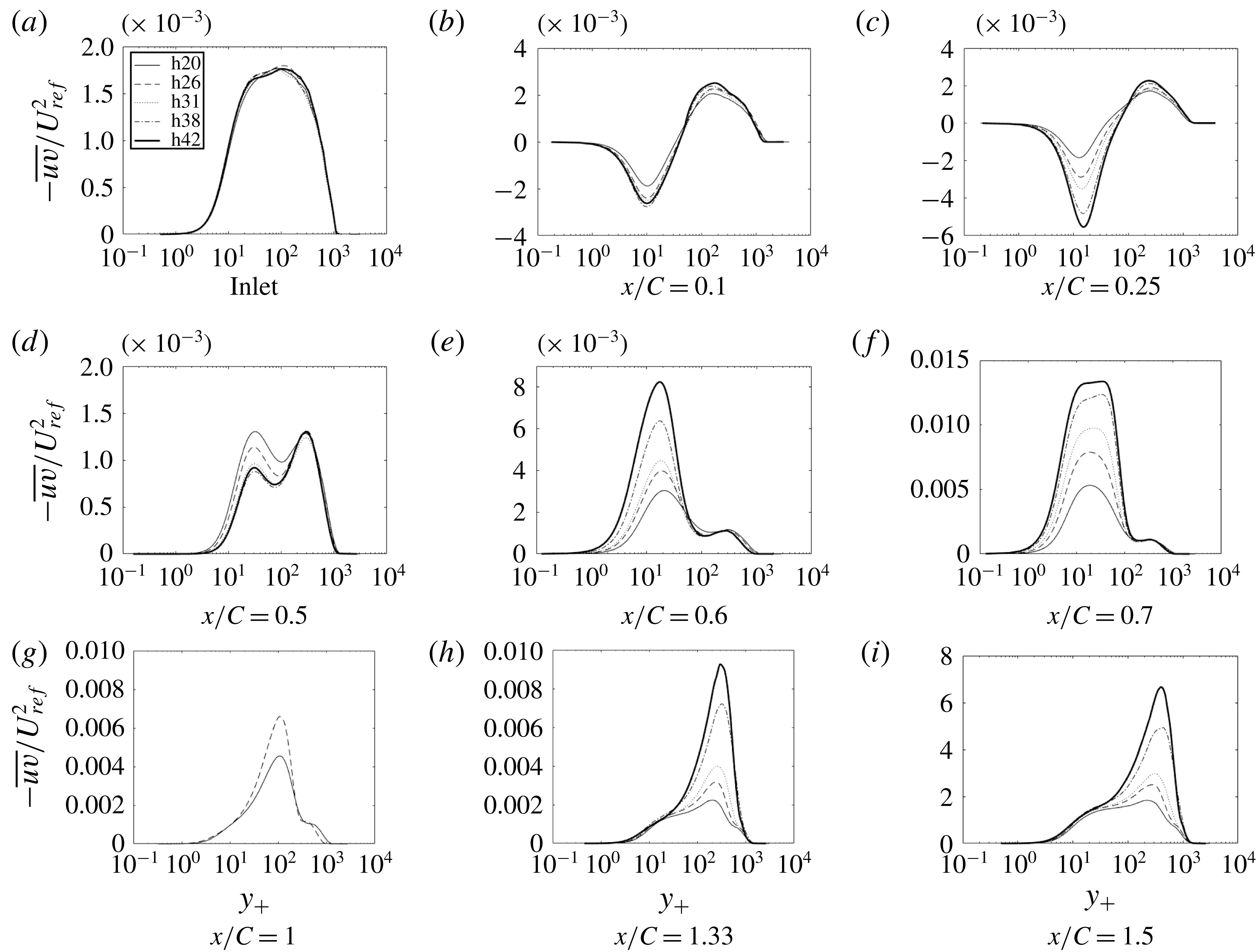
Time- and span-averaged $-\overline{uv}$ at various $x$ locations: ——, h20; - - - -, h26; $\cdots \cdots$ , h31; — - —, h38; _______, h42.

Figure 18.

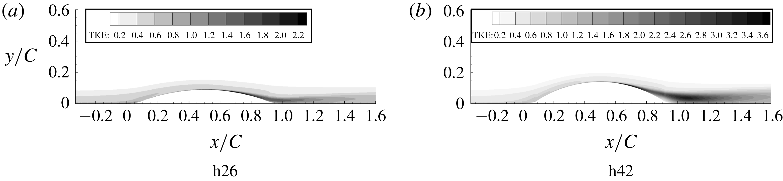
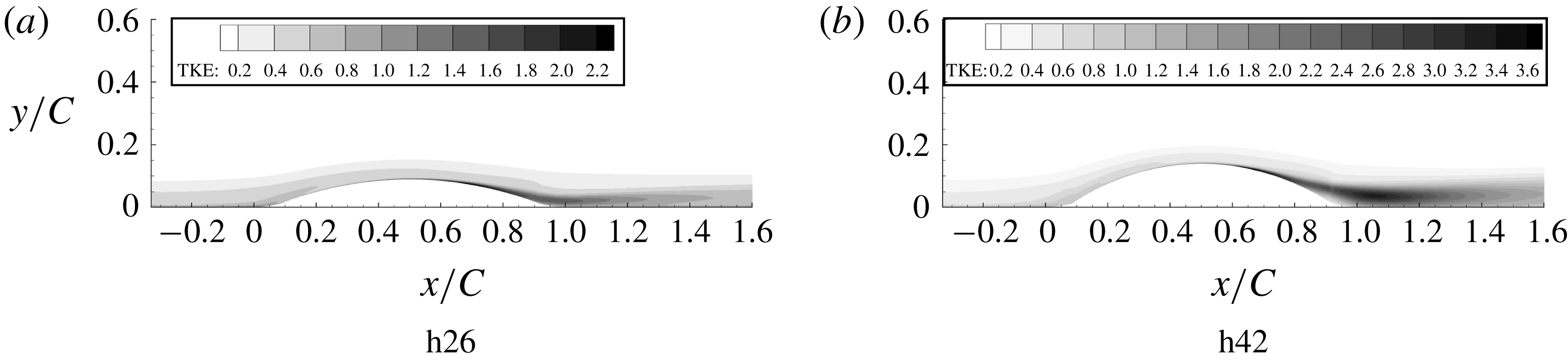
Turbulent kinetic energy contours multiplied by $10^{2}/U_{ref}^{2}$ .

Figure 19.

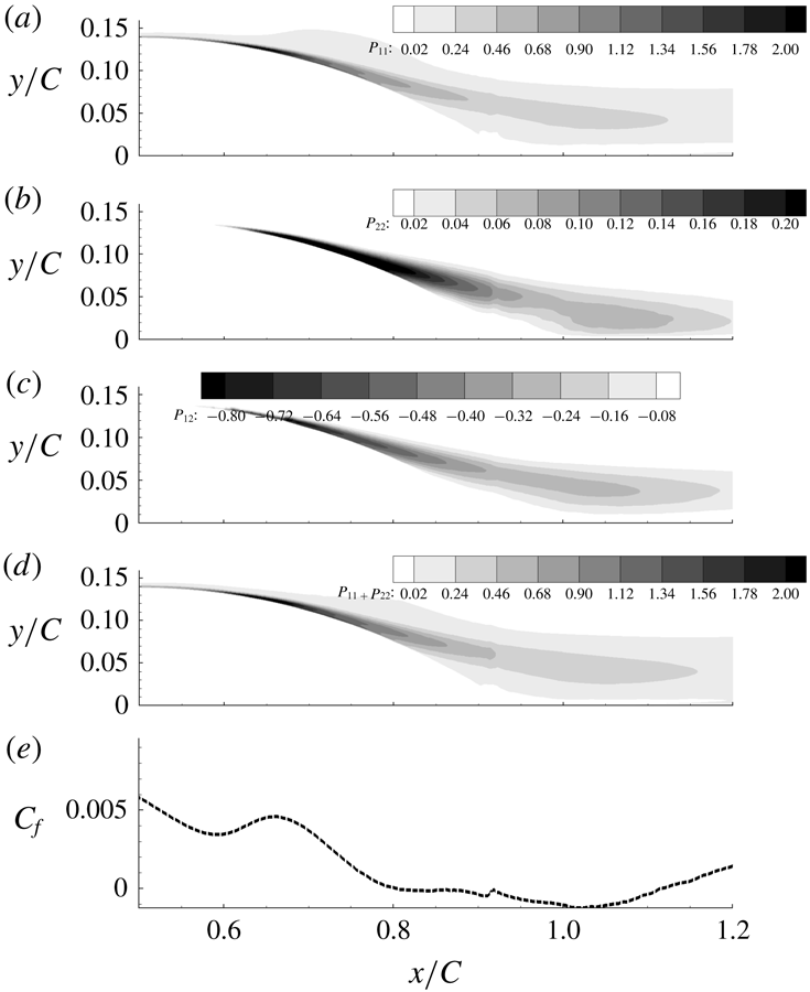
Production tensor component contours for h42 multiplied by $10^{2}\unicode[STIX]{x1D703}/U_{ref}^{3}$ . From the top: $P_{11}$ , $P_{22}$ , $P_{12}$ and $P_{11}+P_{22}$ . Bottom: $C_{f}$ versus $x/C$ is shown for comparison.

The flow over the original bump, h20, did not separate; h26 is on the verge of separation; and h31–h42 develop a small separated region near the end of the bump, as seen in the skin friction coefficient ( $C_{f}$ ) plots in figure 9(a). As the bump height is increased, $C_{f}$ at the bump crest also increases, due to greater flow acceleration; this is exemplified by the $C_{p}$ curves and by the pressure gradient curves in figure 10. Because $P^{+}$ uses $\unicode[STIX]{x1D70F}_{w}$ in the denominator, it behaves erratically in the separated region of the flow.

Pressure gradient parameter $P_{g}$ becomes progressively more negative as the bump height increases. The region of intermittent flow reversal becomes wider and the percentage time the flow is reversed also increases. The maximum flow reversal increases from 25 % of the time for h20 to 100 % of the time for h42. There is also some reversal where the flow encounters APG before the start of the bump. The $C_{f}$ plateau near $x/C=0.7$ becomes a local maximum and a separated region – negative $C_{f}$ – develops near $x/C=0.8$ as the bump height increases.

To test the sensitivity to incident boundary layer thickness, two additional momentum thicknesses equal to $C/52$ (momentum thickness 2) and $C/101$ (momentum thickness 3) were prescribed at the inlet. The effect of the change in momentum thickness is shown in figure 11. The $C_{f}$ and $C_{p}$ profiles remain qualitatively similar; thus, the qualitative behaviour is not sensitive to inlet boundary layer thickness.

The instantaneous skin friction coefficient in a $z$ -plane and its surface contours are plotted in figure 12. The contours show streaky structures and the line plots show turbulent structures, showing that the flow did not relaminarize, even over the highest bump.

Figure 13 provides the streamwise mean velocity profiles in viscous units (note that the viscous units were based on local friction velocity). As in the base simulation, major departure from the log law can be seen over the bump. From figure 10 it is seen that the flow changes from APG to FPG around $x/C=0.08$ and an immediate deviation from the log law is observed. Profiles after $x/C=0.1$ show similarity to reverse transitional profiles; i.e. we see an increase in the thickness of the viscous sublayer that becomes greater as the bump height increases. However, as noted earlier, the flow is never laminar. It is interesting to note that this thick viscous sublayer continues, even after the pressure gradient changes signs (FPG turns to APG) at $x/C=0.5$ . The present simulations parallel behaviours seen over flat and curved surfaces (Tsuji & Morikawa Reference Tsuji and Morikawa1976): in the experiments of Tsuji & Morikawa (Reference Tsuji and Morikawa1976), APG did not result in deviation from the log law, but FPG did.

The profiles progressively deviate from h20 and major deviations can be seen after $y_{+}=10$ . At $x/C=1$ profiles have not been plotted for cases in which the flow separated, because $C_{f}$ is negative. After the bump all the profiles tend towards h20. But, by the end of the domain, the flow has not fully recovered to a ZPG boundary layer.

Figures 14–17 show components of the Reynolds stress tensor for the complete set of bumps. As before, $\overline{uu}$ is the largest diagonal component of the stress tensor; i.e. it is the major contributor to the turbulent kinetic energy (TKE), with its highest value being an order of magnitude larger than those of $\overline{vv}$ and $\overline{ww}$ .

The $\overline{uu}$ profiles show that increasing the crest height decreases the first peak, at around $y_{+}=10$ , and increases the outer peak, at $x/C=0.1$ . Over the crest and in the APG, the inner peak forms into a plateau. The outer peaks are much higher for bumps with higher crest height.

The other components of Reynolds stress develop a similar pattern of near-wall and outer peaks, each component differing in where they develop and in their relative heights, as seen in figures 15–17.

An overview of the field of TKE is provided by contour plots in figure 18. This is especially interesting because the pattern shown has a large effect on skin friction and has a relevance to turbulence closure models. The prominent feature in the contour plots is a band of high TKE that originates near the wall, on the lee side. It originates close to the position where the $C_{f}$ plateau is observed in figure 9 and extends downstream over the recovery region. The band extends further downstream for higher bumps and the magnitude also increases; note that this is not a region of separated flow. While that behaviour seems extraordinary, it was seen in RANS computations with eddy viscosity, as well. The primary departure of RANS from LES was that the band originated farther from the wall. A consequence is that the RANS prediction of $C_{f}$ is inaccurate, as will be seen in figure 20. The LES data provide an insight into the dominant role of near-wall behaviour.

The production of $\overline{uu}$ for h42 is an order of magnitude larger than $\overline{vv}$ , as shown in figure 19. All the production components start near the wall and extend into the recovery region. It can be seen that the streamwise position of this increase coincides, almost perfectly, with the increase in $C_{f}$ . Full budgets (Matai Reference Matai2018) show that in the near-wall $(y_{+}<20)$ APG region, turbulent transport can be more than 50 % as high as production. Thus, turbulent transport is a major contributor to near-wall TKE.

4 Data extraction by inversion

The ambiguous connection between model variables and measurable quantities has been a juggernaut to using data to improve RANS models. Obvious examples are the eddy viscosity and $\unicode[STIX]{x1D714}$ , of the $k$ – $\unicode[STIX]{x1D714}$ model: these are not measurable variables; they exist as artifacts of the closure model. But, even $k$ , as used in the $k{-}\unicode[STIX]{x1D714}$ and $k{-}\unicode[STIX]{x1D716}$ models, does not correspond to turbulent kinetic energy; for example, it equals $3.3u_{\ast }^{2}$ in the log layer, while the actual TKE is higher and depends on Reynolds number (Durbin & Reif Reference Durbin and Reif2011). Duraisamy et al. (Reference Duraisamy, Zhang and Singh2015) proposed an innovative method to extract data on model variables by solving an optimization problem. (We gratefully acknowledge Professor Duraisamy for providing the computer code to do this.)

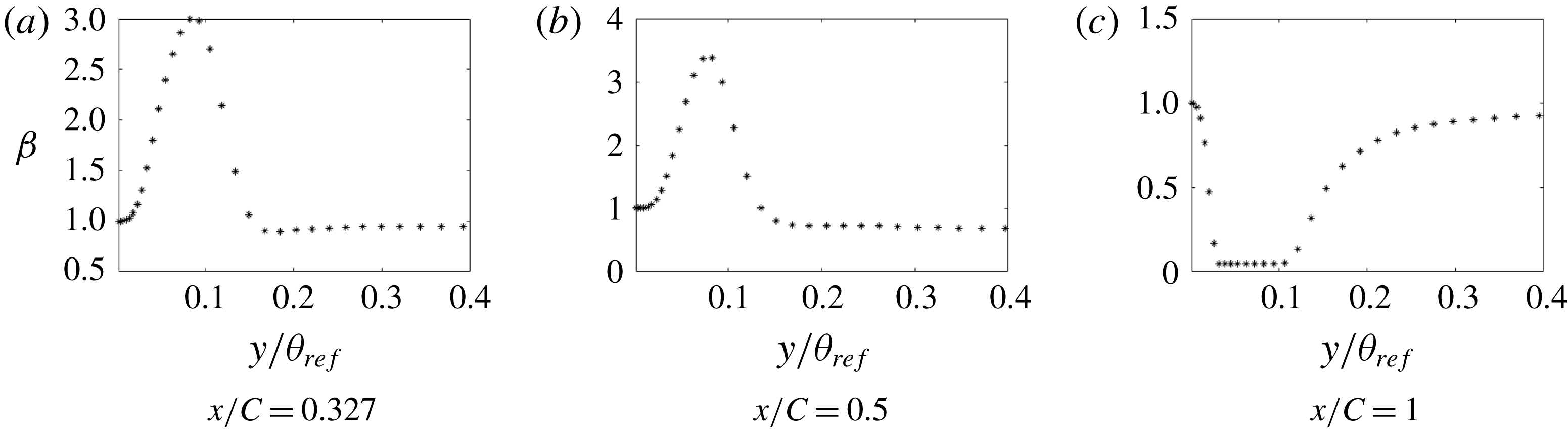
In the method of Duraisamy et al. (Reference Duraisamy, Zhang and Singh2015), optimization is accomplished after introducing a coefficient into the $k{-}\unicode[STIX]{x1D714}$ model. The coefficient can be inserted in various places. Here, the production term of the $\unicode[STIX]{x1D714}$ equation is multiplied by a coefficient $\unicode[STIX]{x1D6FD}$ :

(4.1)

$$\begin{eqnarray}\frac{\text{D}\unicode[STIX]{x1D714}}{\text{D}t}=\unicode[STIX]{x1D6FD}(\boldsymbol{x})\,c_{\unicode[STIX]{x1D714}1}|S|^{2}-c_{\unicode[STIX]{x1D714}2}\unicode[STIX]{x1D714}^{2}+\unicode[STIX]{x1D735}\boldsymbol{\cdot }(\unicode[STIX]{x1D708}+\unicode[STIX]{x1D70E}_{\unicode[STIX]{x1D714}}k/\unicode[STIX]{x1D714})\unicode[STIX]{x1D735}\unicode[STIX]{x1D714},\end{eqnarray}$$

where $\unicode[STIX]{x1D6FD}$ is initialized to the baseline value of unity. Then values of $\unicode[STIX]{x1D6FD}$ over the grid are found by minimizing a cost function, $J$ . Two cost functions were examined: the surface skin friction, and the $x$ -velocity profiles; either

(4.2a,b )

$$\begin{eqnarray}J=\sum (\mathop{C}_{f}^{RANS}-C_{f}^{LES})^{2}A_{face}\quad \text{or}\quad J=\sum (U^{RANS}-U^{LES})^{2}\frac{V_{cell}}{d_{w}^{2}},\end{eqnarray}$$

where $d_{w}$ is wall distance. Inverse wall distance weighting was used in (4.2) to compensate the small values of $U$ near the wall.

The optimization problem is $(\unicode[STIX]{x1D6FD}(x,y)\,\mid \,\min _{\unicode[STIX]{x1D6FD}}J)$ . Minimization is accomplished iteratively, requiring the full RANS equations to be solved at each iteration. A gradient descent algorithm is used to reach the optimum solution. The gradient of the cost ( $\unicode[STIX]{x2202}J/\unicode[STIX]{x2202}\unicode[STIX]{x1D6FD}$ ), which represents its sensitivity to $\unicode[STIX]{x1D6FD}$ , is calculated by solving a linear adjoint set of equations (see Duraisamy et al. (Reference Duraisamy, Zhang and Singh2015) for a more complete discussion).

Figure 20.

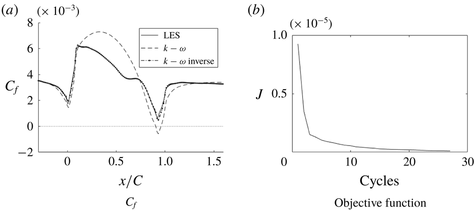
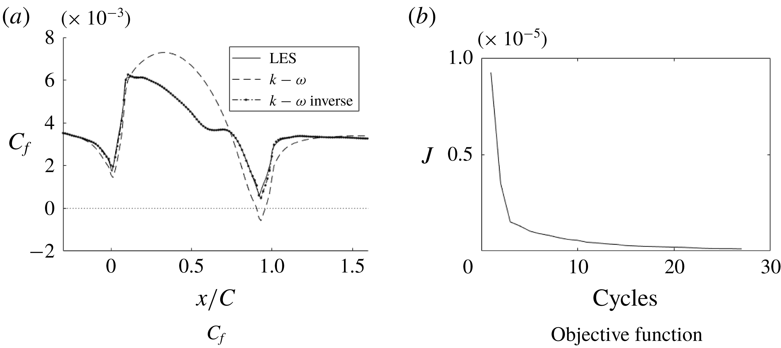
Skin friction coefficient $C_{f}$ of the inverse solution compared to LES and RANS solutions and the objective function for the optimization (h20).

Figure 21.

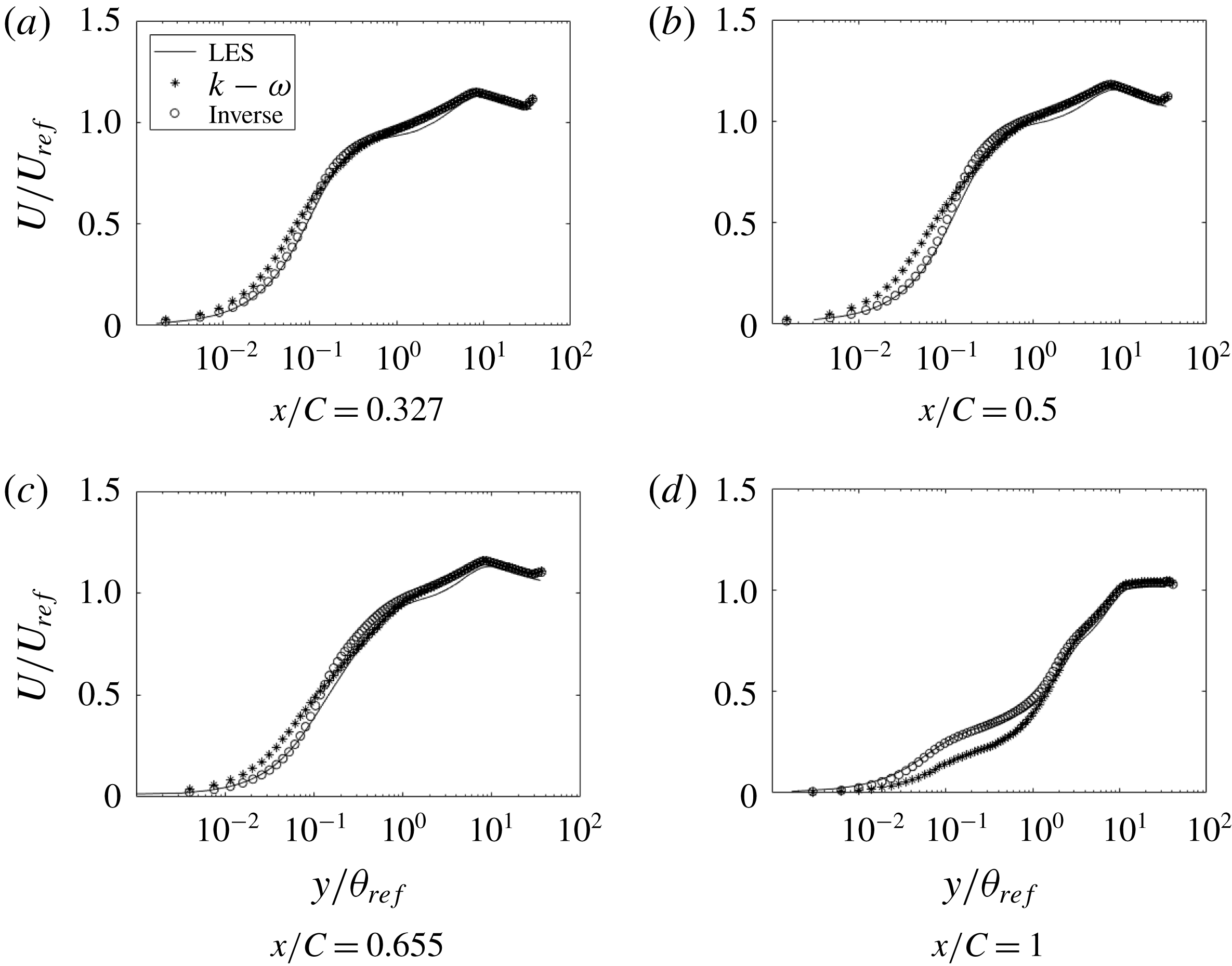
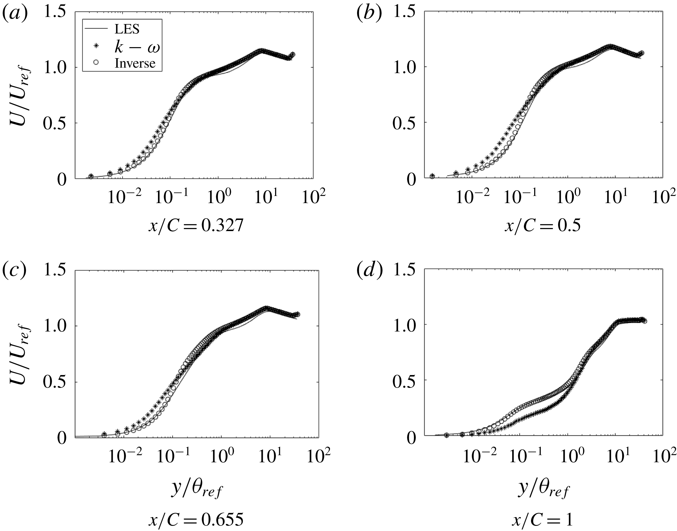
Comparison of streamwise velocity at various $x$ locations (h20): $\ast$ , base model; $\circ$ , optimized; ——, LES.

Figure 22.

Correction profiles ( $\unicode[STIX]{x1D6FD}$ ) at various $x$ locations (h20).

Figure 23.

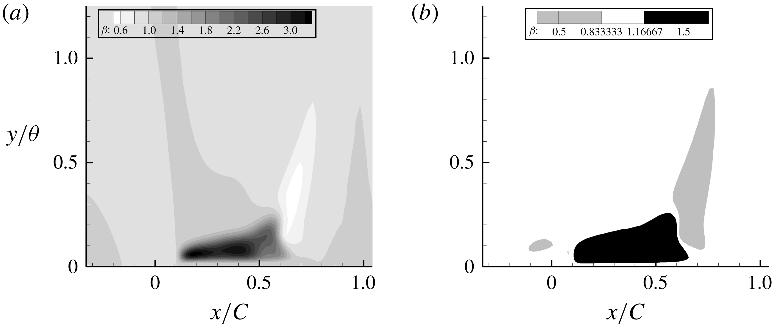
Distribution of $\unicode[STIX]{x1D6FD}$ for h42. The $y$ -coordinate is relative to the surface.

Figure 24.

Comparison of $\unicode[STIX]{x1D708}_{t}$ at various $x$ locations (h20): $\ast$ , base model; $\circ$ , optimized.

Figure 25.

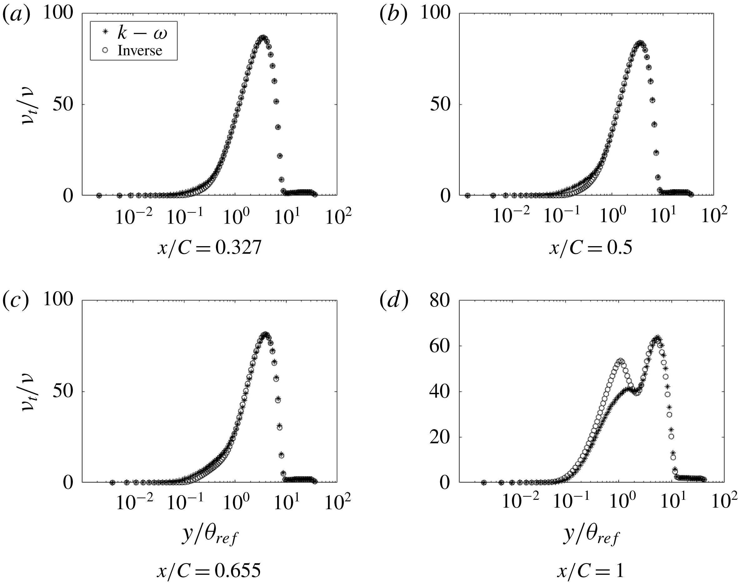
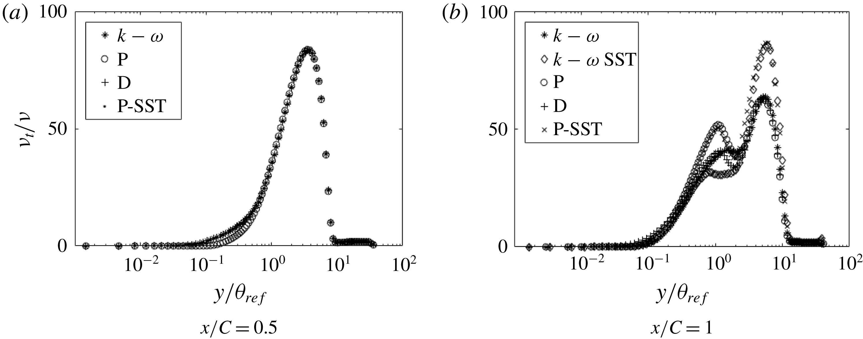
Comparison of inverse solutions with different base models and with the correction factor multiplied to the destruction of $\unicode[STIX]{x1D714}$ term instead of production (h20): $\ast$ , base $k$ – $\unicode[STIX]{x1D714}$ model; $\diamond$ , base $k$ – $\unicode[STIX]{x1D714}$ SST model; $\circ$ , $\unicode[STIX]{x1D6FD}$ multiplied to production of $\unicode[STIX]{x1D714}$ of base $k$ – $\unicode[STIX]{x1D714}$ model; $+$ , $\unicode[STIX]{x1D6FD}$ multiplied to destruction of $\unicode[STIX]{x1D714}$ of base $k$ – $\unicode[STIX]{x1D714}$ model; $\times$ , $\unicode[STIX]{x1D6FD}$ multiplied to production of $\unicode[STIX]{x1D714}$ of base $k$ – $\unicode[STIX]{x1D714}$ SST model.

Figure 26.

Comparison of streamwise velocity at various $x$ locations for inverse solutions with different cost functions (h20).

Figure 27.

Comparison of $\unicode[STIX]{x1D708}_{t}$ at various $x$ locations for inverse solutions with different cost functions (h20).

Figure 28.

Comparison of $k$ at various $x$ locations (h20).

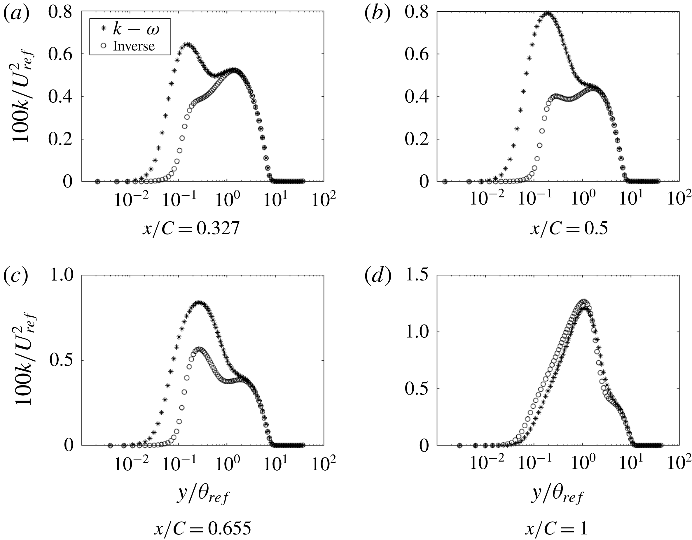
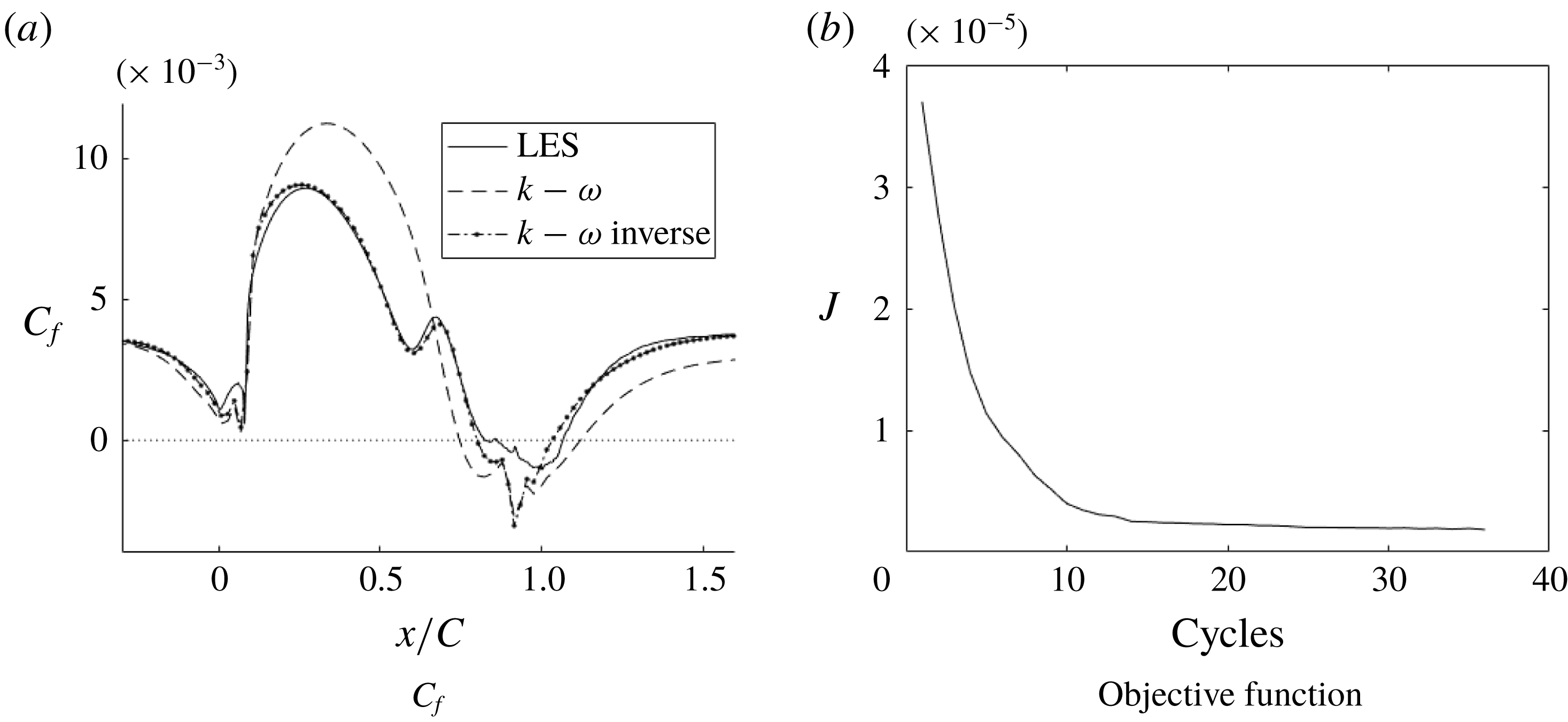
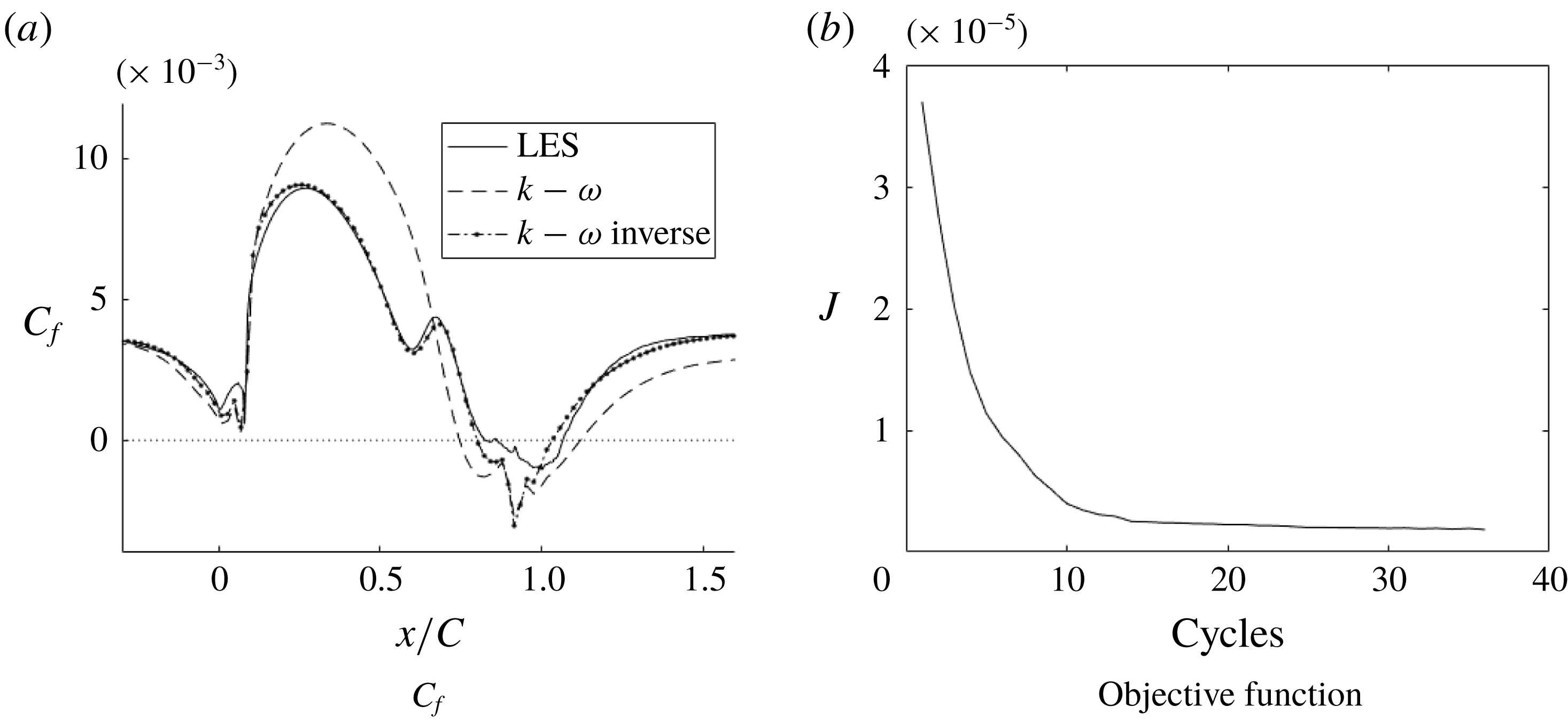
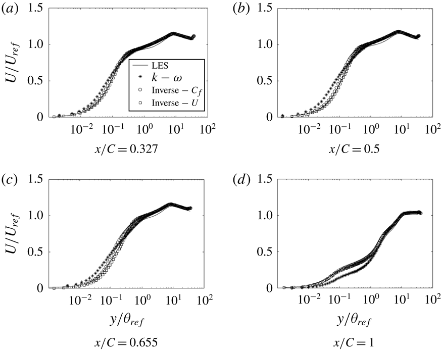
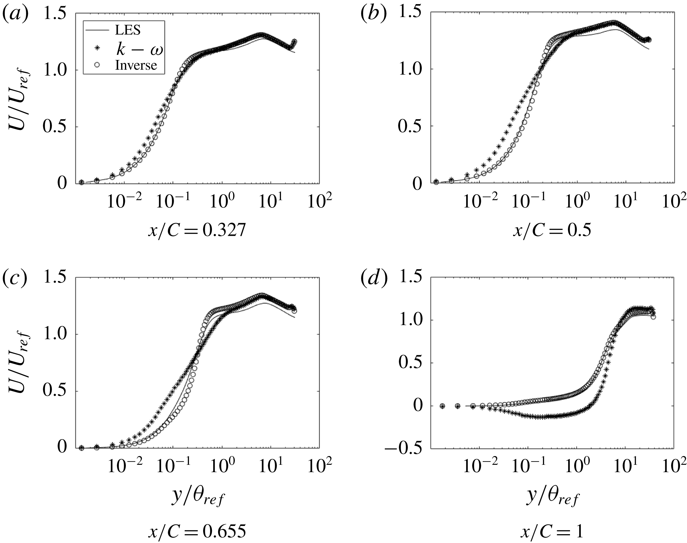
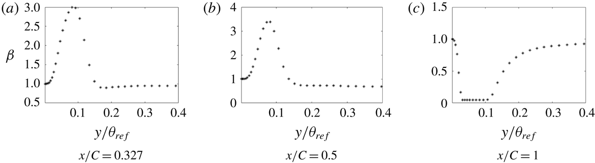
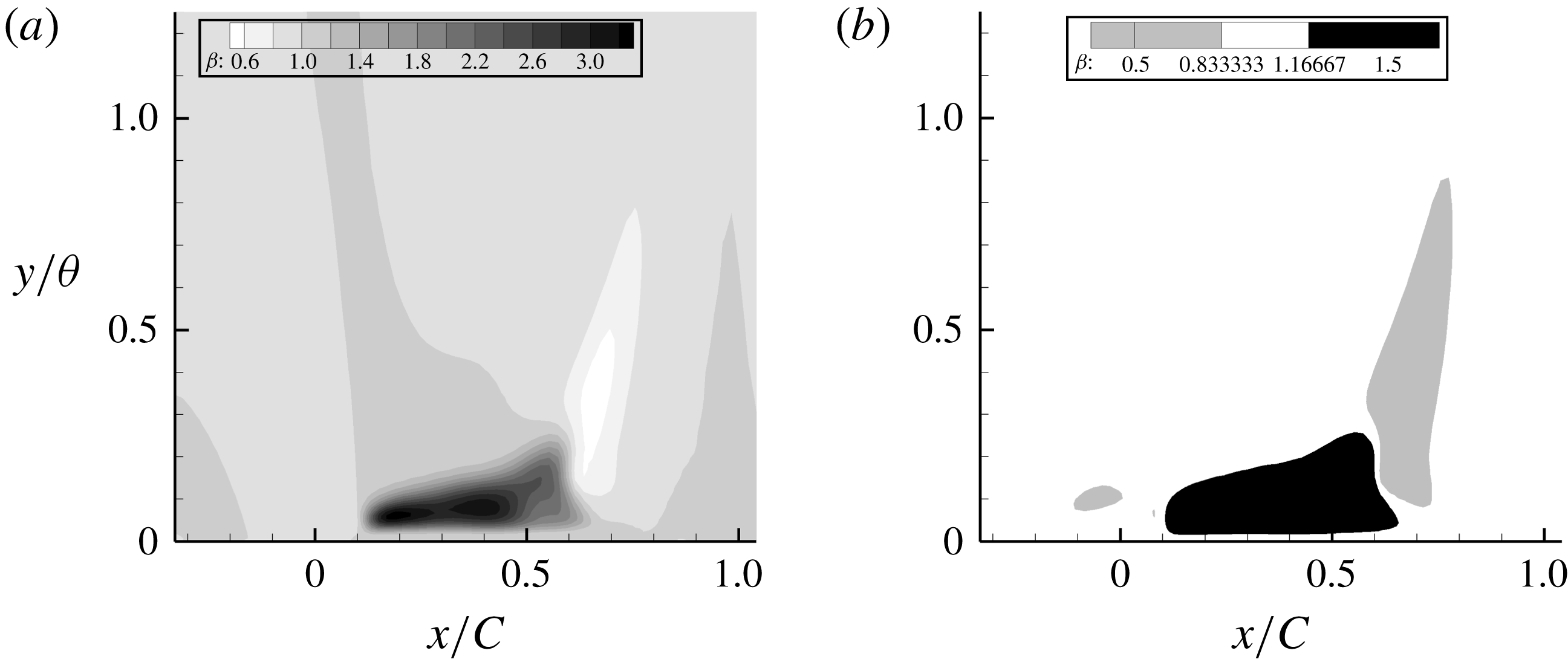
Figure 20 shows that, once the optimal field $\unicode[STIX]{x1D6FD}(x,y)$ was reached, the $C_{f}$ matched almost exactly with the LES data. Figure 21 shows that, even with $C_{f}$ as the cost function, the velocity profiles match well with the LES data; thus, although the cost function is a wall quantity, its effect on the solution is not local. Figure 22 shows that corrections are needed, mostly near the wall. Contour plots for case h42, figure 23, show that $\unicode[STIX]{x1D6FD}>1$ is needed in the FPG and $\unicode[STIX]{x1D6FD}<1$ in the APG case. The former enhances $\unicode[STIX]{x1D714}$ , hence reducing the eddy viscosity $k/\unicode[STIX]{x1D714}$ , and vice versa. This can be seen clearly in figure 23(b).

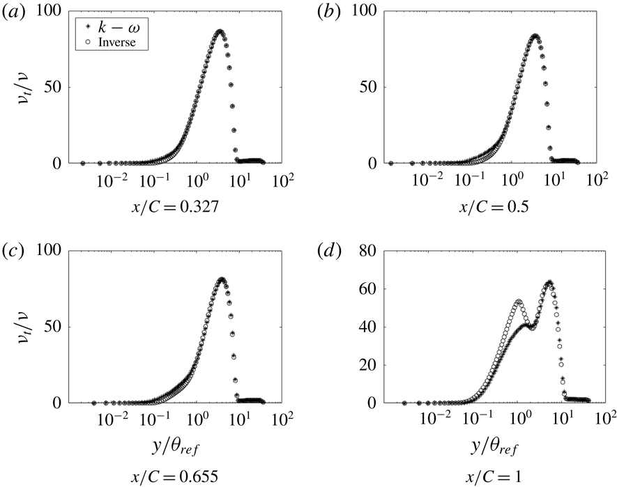
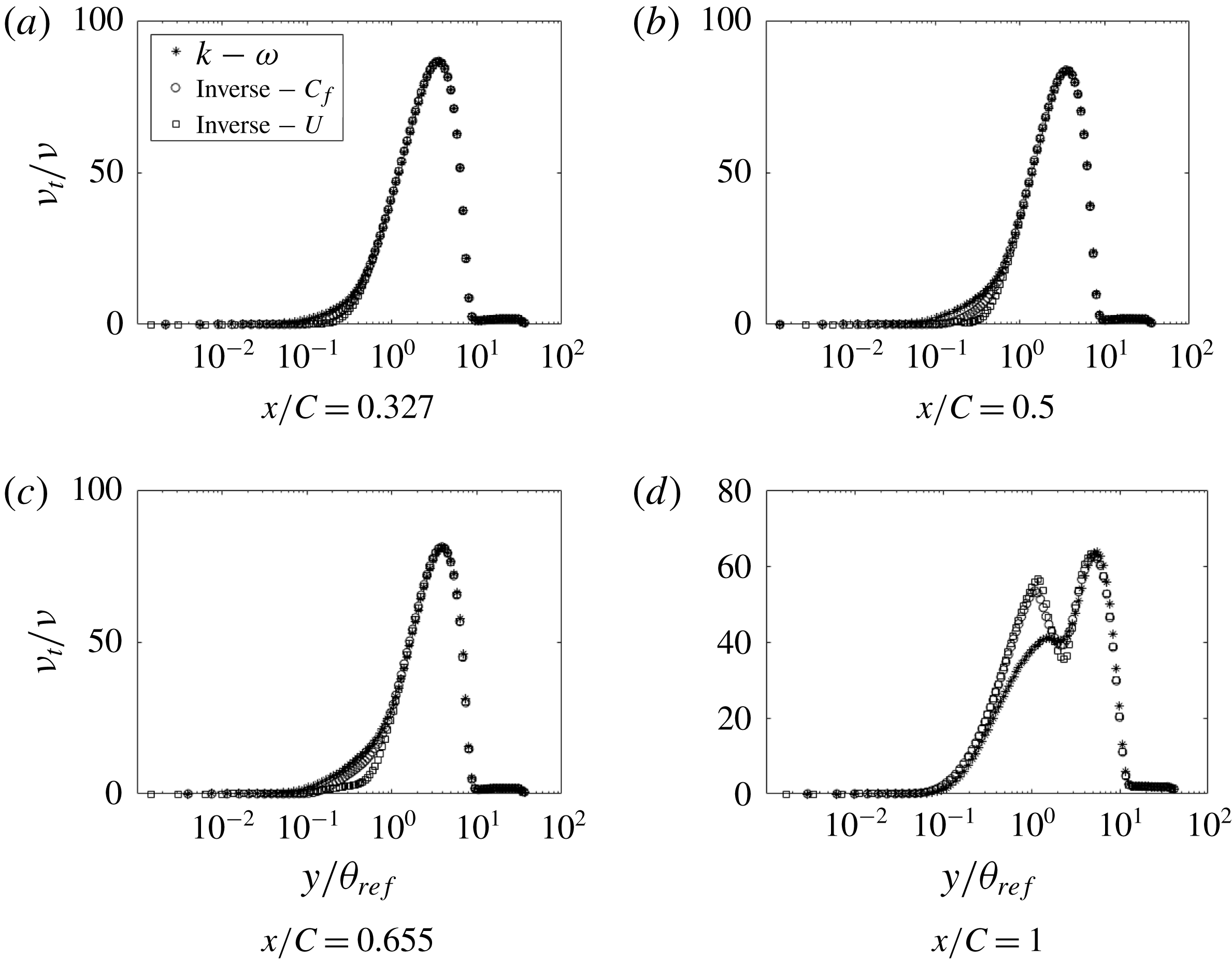
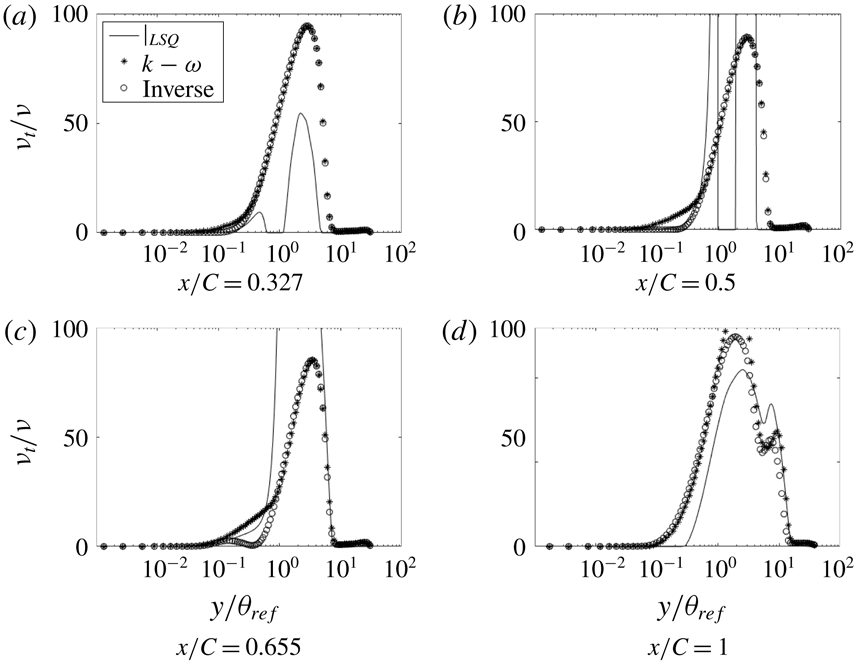
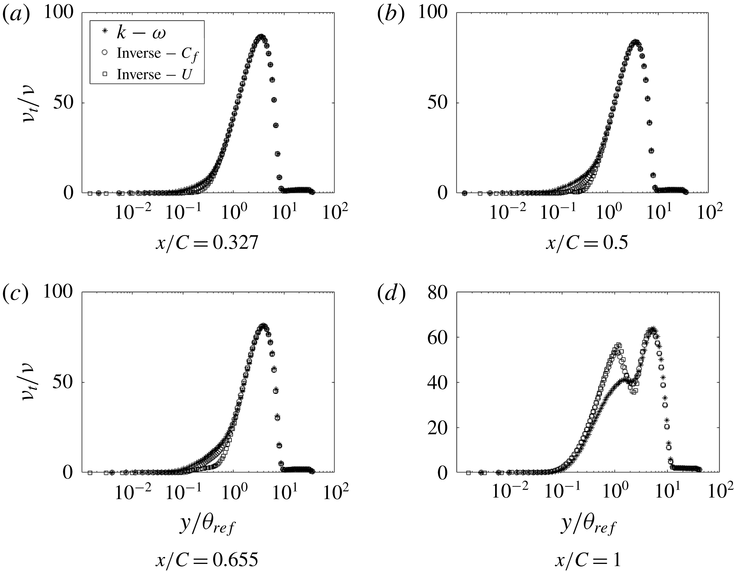
We regard the eddy viscosity, obtained in this manner, to be data; albeit, data that are extracted, not measured directly. Figure 24 shows the initial eddy viscosity, corresponding to $\unicode[STIX]{x1D6FD}=1$ , and the optimized eddy viscosity. It can be seen that most of the difference between the two is near the wall, below $y/\unicode[STIX]{x1D703}_{ref}=1$ ( $y/\unicode[STIX]{x1D703}_{ref}=1$ corresponds to $y_{+}\approx 100$ ). On the FPG side, the baseline model overpredicts the eddy viscosity. This trend continues for some distance even after the pressure gradient reverses its sign, suggesting a lag effect. At the end of the bump, the baseline model underpredicts the eddy viscosity near the wall. One can attribute failures of the baseline $k{-}\unicode[STIX]{x1D714}$ model largely to erroneous eddy viscosity quite near the wall.

Although it might appear that the optimal and baseline viscosity are the same when $y/\unicode[STIX]{x1D703}_{ref}\gtrsim 1$ , they are not; the cost function is insensitive to the eddy viscosity in this region. Regions where the optimal and baseline viscosities are the same are insensitive to the optimizer, and these cannot be trusted as extracted data. This points to a limitation of the present method. The data that it provides on turbulence variables are significant only where those data differ from the baseline model.

This is illustrated by changing the baseline model to the $k{-}\unicode[STIX]{x1D714}$ shear stress transport (SST) model, with the corrector term, $\unicode[STIX]{x1D6FD}$ , again multiplying the production of $\unicode[STIX]{x1D714}$ . Figure 25(b) shows the optimal $\unicode[STIX]{x1D708}_{T}/\unicode[STIX]{x1D708}$ for two baseline models. The optima agree when $y/\unicode[STIX]{x1D703}_{ref}\lesssim 1$ . However, dependence on the baseline model is seen further from the wall. The cost function is not sensitive to data at these locations. Hence, the values of $\unicode[STIX]{x1D708}_{t}$ remain the default, i.e. the same as the base model. A corollary to this non-uniqueness is that correct velocity profiles can be obtained using different $\unicode[STIX]{x1D708}_{t}$ distributions; and this is so because the near-wall behaviour has an overwhelming influence on the boundary layer flow.

The sensitivity of the inverse solution to the position of the correction multiplier was checked by moving $\unicode[STIX]{x1D6FD}$ to the destruction term (D in figure 25) of the $\unicode[STIX]{x1D714}$ equation (4.1). Figure 25 shows that the inverse solutions for the eddy viscosity are virtually identical.

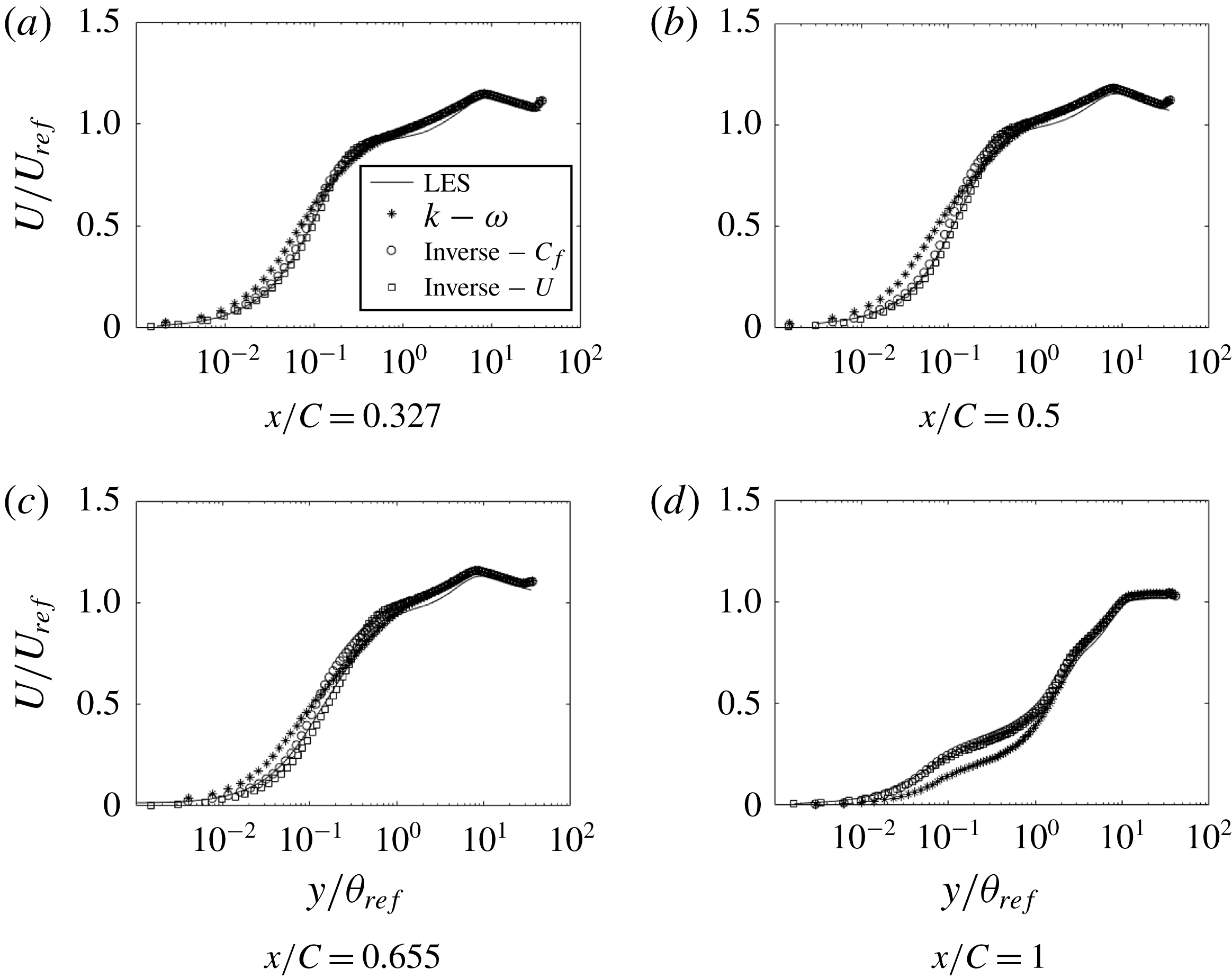
The effect of the cost function on the inverse solution was examined by using the second cost function in (4.2). Figure 26 shows the velocity profile for both the cost functions. A small difference is visible only at $x/C=0.655$ . The eddy viscosity profiles show some differences (figure 27), suggesting a non-unique optimum eddy viscosity. Near the end of the bump they become identical. Of the two, the $C_{f}$ cost function seems preferable.

Figure 29.

Cost function $C_{f}$ of the inverse solution compared to LES and RANS solutions and the objective function for the optimization (h38).

Figure 30.

Comparison of streamwise velocity at various $x$ locations (h38).

Figure 31.

Comparison of $\unicode[STIX]{x1D708}_{t}$ at various $x$ locations (h38): $\ast$ , base model; $\circ$ , optimized; ——, least squares.

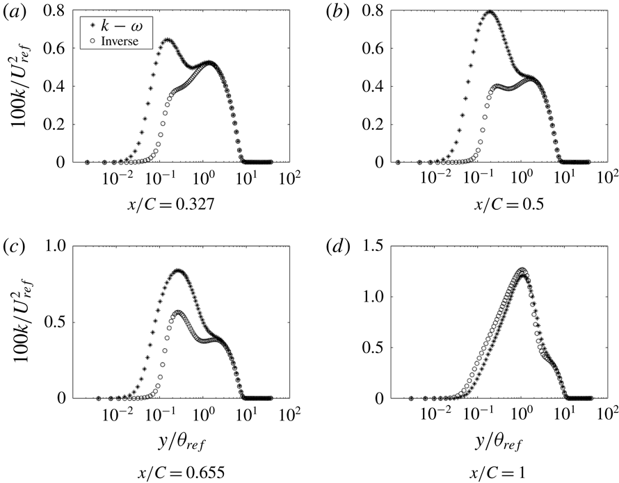
The variable $k$ shows a trend similar to the eddy viscosity since they are directly proportional (figure 28). In the FPG section of the bump, $k$ is overpredicted by the baseline RANS solution. The baseline also predicts a spurious peak near the wall, which does not exist in the optimal solution.

A similar optimization procedure was carried out for h38, and is shown in figure 29. The inverse solution matches almost exactly with the LES data, except very near the end of the bump. At this point the gradients become exceedingly small and the optimization does not converge to the data. Elsewhere, it is quite accurate. Figure 30 shows the optimal solution agreeing well with the LES data, again proving that optimizing the $C_{f}$ cost function can correct the velocity field away from the wall.

One might propose a simpler extraction of eddy viscosity. Least-squares minimization of the eddy viscosity in the formula

(4.3)

$$\begin{eqnarray}\overline{u_{i}u}_{j}=-2\unicode[STIX]{x1D708}_{t}S_{ij}+{\textstyle \frac{3}{2}}k\unicode[STIX]{x1D6FF}_{ij}\end{eqnarray}$$

gives

(4.4)

$$\begin{eqnarray}\unicode[STIX]{x1D708}_{t}=-\frac{\overline{u_{i}u}_{j}S_{ij}}{2S_{ij}S_{ij}}.\end{eqnarray}$$

Inserting LES data on the right extracts an eddy viscosity. Note, however, that this is not a rational method; there is no connection between least squares and the operational use of eddy viscosity. Figure 31 shows that the eddy viscosity from least squares agrees with the inverse solution near the wall at some locations. However, in general, it is quite unreasonable.

5 Conclusion

The present is an empirical study. LES was used to create flow over a set of five bumps, with increasing crest heights. The influence of pressure gradients on the turbulence is brought out through comparisons within this family. The base case, with the lowest bump height, had been studied experimentally by Webster et al. (Reference Webster, Degraaff and Eaton1996) and the LES were validated with their data. Conversely, the LES fills in omissions from laboratory data, providing a more complete picture of the flow field for the reference bump.

The lowest bump had no separation, while, the highest bump produced a marginal separation. The grid requirements are the most severe for the highest bump. To ensure solution accuracy, a convergence study was carried out for that case. For LES, grid refinement studies provide a measure of ‘experimental uncertainty’. The grid that was used in the present simulations provides a benchmark degree of accuracy. A database for the bump series is available at Rumsey (Reference Rumsey2018).

The Reynolds stress data show some intriguing behaviours. All components of the Reynolds stress developed second peaks over the bump. A detached layer of high TKE developed in the wake. This is distinct from high TKE in fully separated flow. Even in the marginally separated cases, the band of high TKE leaves the surface well before separation. The band is due to the mean shear profile created by adverse pressure gradient.

A plateau in the skin friction develops into a local maximum on the lee side (figure 9), as the bump height increases. In combination with the band of high TKE, this is seen to be a consequence of the reaction of the Reynolds stresses to the flow field, and not a direct effect of the pressure distribution.

These and other effects of strong disequilibrium, such as the absence of a log layer, prevent data correlation. Hence, the parametric series provides a systematic view of the development of disequilibrium. Although the focus is on adverse pressure gradient, there is flow acceleration over the front slope of the bump. In that region, turbulent intensity is initially reduced near the wall – increasingly so as the bump height increases. However, the flow remains fully turbulent. There has been some question over whether the flow relaminarizes: it does not, even for the highest bump.

The database was originally created for assessment and development of Reynolds-averaged models. It was shown that RANS with $k$ – $\unicode[STIX]{x1D714}$ fails to correctly simulate flow over these bumps. In order to explore the origin of this failure, turbulence variables were extracted by an optimization procedure. The extracted data include the eddy viscosity, $\unicode[STIX]{x1D708}_{t}$ . It was shown that current turbulence models fail because their predicted eddy viscosity is erroneous close to the wall. The behaviour of the eddy viscosity further away from the wall did not have an appreciable effect on the flow solution.

Acknowledgements

This work was funded in part by the National Science Foundation Grant no. 1507928, NASA grant NNX15AN98A and Office of Naval Research award no. N00014-17- 1-2200. We are grateful to Professor K. Duraisamy for his help.

References

Alving, A. E., Smits, A. J. & Watmuff, J. H. 1990 Turbulent boundary layer relaxation from convex curvature. J. Fluid Mech. 211, 529–556.10.1017/S0022112090001689Google Scholar

Arolla, S. K. 2016 Inflow turbulence generation for eddy-resolving simulations of turbomachinery flows. J. Fluids Engng 138 (3), 031201.Google Scholar

Bandyopadhyay, P. R. & Ahmed, A. 1993 Turbulent boundary layers subjected to multiple curvatures and pressure gradients. J. Fluid Mech. 246, 503–527.10.1017/S0022112093000242Google Scholar

Blackwelder, R. F. & Kovasznay, L. S. 1972 Large-scale motion of a turbulent boundary layer during relaminarization. J. Fluid Mech. 53 (1), 61–83.10.1017/S0022112072000047Google Scholar

Breuer, M., Peller, N., Rapp, C. & Manhart, M. 2009 Flow over periodic hills – numerical and experimental study in a wide range of Reynolds numbers. Comput. Fluids 38, 433.10.1016/j.compfluid.2008.05.002Google Scholar

Duraisamy, K., Zhang, Z. J. & Singh, A. P. 2015 New approaches in turbulence and transition modeling using data-driven techniques. In 53rd AIAA Aerospace Sciences Meeting, AIAA Paper 2015–1284.Google Scholar

Durbin, P. A. 2018 Some recent developments in turbulence closure modeling. Annu. Rev. Fluid Mech. 50, 1–27.10.1146/annurev-fluid-122316-045020Google Scholar

Durbin, P. A. & Reif, B. P. 2011 Statistical Theory and Modeling for Turbulent Flows. Wiley.Google Scholar

Matai, R.2018 LES of flow over bumps and machine learning augmented turbulence modeling. PhD thesis, Iowa State University.Google Scholar

Matai, R. & Durbin, P. 2019 Zonal eddy viscosity models based on machine learning. Flow Turbul. Combust., doi:10.1007/s10494-019-00011-5.Google Scholar

Mollicone, J.-P., Battista, F., Gualtieri, P. & Casciola, C. 2017 Effect of geometry and Reynolds number on the turbulent separated flow behind a bulge in a channel. J. Fluid Mech. 823, 100–133.10.1017/jfm.2017.255Google Scholar

Parish, E. J. & Duraisamy, K. 2016 A paradigm for data-driven predictive modeling using field inversion and machine learning. J. Comput. Phys. 305, 758–774.Google Scholar

Patel, V. 1965 Calibration of the Preston tube and limitations on its use in pressure gradients. J. Fluid Mech. 23 (1), 185–208.10.1017/S0022112065001301Google Scholar

Rumsey, C.2018 NASA Turbulence Modeling Resource.https://turbmodels.larc.nasa.gov/Other_LES_Data/family_of_bumps.html.Google Scholar

Seifert, A. & Pack, L. G. 2002 Active flow separation control on wall-mounted hump at high Reynolds numbers. AIAA J. 40 (7), 1363–1372.Google Scholar

Singh, A. P., Matai, R., Mishra, A., Duraisamy, K. & Durbin, P. A. 2017 Data-driven augmentation of turbulence models for adverse pressure gradient flows. In 23rd AIAA Computational Fluid Dynamics Conference, AIAA Paper 2017–3626.Google Scholar

Slotnick, J., Khodadoust, A., Alonso, J., Darmofal, D., Gropp, W., Lurie, E. & Mavriplis, D.2014 CFD vision 2030 study: a path to revolutionary computational aerosciences. NASA. Tech. Rep. CR-2014-218178.Google Scholar

Spalart, P. R. & Watmuff, J. H. 1993 Experimental and numerical study of a turbulent boundary layer with pressure gradients. J. Fluid Mech. 249, 337–371.10.1017/S002211209300120XGoogle Scholar

Tsuji, Y. & Morikawa, Y. 1976 Turbulent boundary layer with pressure gradient alternating in sign. Aeronaut. Q. 27 (1), 15–28.10.1017/S0001925900007514Google Scholar

Webster, D., Degraaff, D. & Eaton, J. 1996 Turbulence characteristics of a boundary layer over a two-dimensional bump. J. Fluid Mech. 320, 53–69.10.1017/S0022112096007458Google Scholar

Weller, H. G., Tabor, G., Jasak, H. & Fureby, C. 1998 A tensorial approach to computational continuum mechanics using object-oriented techniques. Comput. Phys. 12 (6), 620–631.10.1063/1.168744Google Scholar

Wu, X. & Squires, K. D. 1998 Numerical investigation of the turbulent boundary layer over a bump. J. Fluid Mech. 362, 229–271.10.1017/S0022112098008982Google Scholar

Figure 1.Mesh used for the LES simulation, shown for the h20 reference bump. Note the disconnected recycling domain for generating the inlet flow ($C=0.305$ m).

Figure 2.Grid convergence for highest bump (h42), LES: ——, mesh 1; - - - -, mesh 2; $\cdots \cdots$, mesh 3; — - —, mesh 4.

Table 1.Grid characteristics of the bump simulation at $Re_{\unicode[STIX]{x1D703}}=2500$.

Figure 3.Time- and span-averaged $x$-velocity at various $x$ locations: ——, LES; $\ast$, experiment.

Figure 4.Time- and span-averaged $\overline{uu}$ at various $x$ locations: ——, LES; — - —, single wire; $\ast$, X-wire.

Figure 5.Time- and span-averaged $\overline{vv}$, $\overline{ww}$ and $-\overline{uv}$ at various $x$ locations normalized by $U_{ref}^{2}$: ——, LES; $\ast$, experiment.

Figure 6.Pressure coefficient, pressure gradient parameters and intermittent flow reversal at the wall.

Figure 7.Skin friction coefficient.

Figure 8.Bump geometries.

Table 2.Summary of bumps.

Figure 9.Comparison of skin friction coefficient and pressure for different bump crest heights.

Figure 10.Pressure gradient parameters and intermittent flow reversal at the wall for bumps with different crest heights.

Figure 11.Comparison of skin friction coefficient and pressure for different inlet momentum thicknesses (h20).

Figure 12.Instantaneous skin friction coefficient for h42.

Figure 13.Time- and span-averaged $x$-velocity at various $x$ locations: ——, h20; - - - -, h26; $\cdots \cdots$, h31; — - —, h38; _______, h42.

Figure 14.Time- and span-averaged $\overline{uu}$ at various $x$ locations: ——, h20; - - - -, h26; $\cdots \cdots$, h31; — - —, h38; _______, h42.

Figure 15.Time- and span-averaged $\overline{vv}$ at various $x$ locations: ——, h20; - - - -, h26; $\cdots \cdots$, h31; — - —, h38; _______, h42.

Figure 16.Time- and span-averaged $\overline{ww}$ at various $x$ locations: ——, h20; - - - -, h26; $\cdots \cdots$, h31; — - —, h38; _______, h42.

Figure 17.Time- and span-averaged $-\overline{uv}$ at various $x$ locations: ——, h20; - - - -, h26; $\cdots \cdots$, h31; — - —, h38; _______, h42.

Figure 18.Turbulent kinetic energy contours multiplied by $10^{2}/U_{ref}^{2}$.

Figure 19.Production tensor component contours for h42 multiplied by $10^{2}\unicode[STIX]{x1D703}/U_{ref}^{3}$. From the top: $P_{11}$, $P_{22}$, $P_{12}$ and $P_{11}+P_{22}$. Bottom: $C_{f}$ versus $x/C$ is shown for comparison.

Figure 20.Skin friction coefficient $C_{f}$ of the inverse solution compared to LES and RANS solutions and the objective function for the optimization (h20).

Figure 21.Comparison of streamwise velocity at various $x$ locations (h20): $\ast$, base model; $\circ$, optimized; ——, LES.

Figure 22.Correction profiles ($\unicode[STIX]{x1D6FD}$) at various $x$ locations (h20).

Figure 23.Distribution of $\unicode[STIX]{x1D6FD}$ for h42. The $y$-coordinate is relative to the surface.

Figure 24.Comparison of $\unicode[STIX]{x1D708}_{t}$ at various $x$ locations (h20): $\ast$, base model; $\circ$, optimized.

Figure 25.Comparison of inverse solutions with different base models and with the correction factor multiplied to the destruction of $\unicode[STIX]{x1D714}$ term instead of production (h20): $\ast$, base $k$–$\unicode[STIX]{x1D714}$ model; $\diamond$, base $k$–$\unicode[STIX]{x1D714}$ SST model; $\circ$, $\unicode[STIX]{x1D6FD}$ multiplied to production of $\unicode[STIX]{x1D714}$ of base $k$–$\unicode[STIX]{x1D714}$ model; $+$, $\unicode[STIX]{x1D6FD}$ multiplied to destruction of $\unicode[STIX]{x1D714}$ of base $k$–$\unicode[STIX]{x1D714}$ model; $\times$, $\unicode[STIX]{x1D6FD}$ multiplied to production of $\unicode[STIX]{x1D714}$ of base $k$–$\unicode[STIX]{x1D714}$ SST model.