1. INTRODUCTION
Many statistical and econometric data sets exhibit some form of truncation. In this paper we consider estimation of a truncated regression model, which corresponds to a regression model where the sample is selected on the basis of the dependent variable.
1See, e.g., Hausman and Wise (1977) and Wooldridge (2002) for empirical examples of this type of sampling.

, wi, and ei denote a latent dependent variable, a J + 1–dimensional vector of observed covariates (which may include a constant), and a random unobserved disturbance term. We have the following latent variable relationship:

For our truncated model the econometrician does not observe

, but the nonnegative variable yi, where

If

were observed without truncation, then it could be linearly regressed on wi using ordinary or two-stage least squares to estimate θ0, which is the parameter of interest. However, this simple estimator cannot be used because our data are only sampled from individuals having

positive.
Our method of obtaining identification makes relatively weak assumptions regarding ei, but it assumes that we can estimate the population (as opposed to the truncated) distribution of the regressors wi. One way this may be accomplished is by having two distinct data sets, one being a sample of yi, wi observations generated by the truncation model

and the other a possibly independent sample of just wi observations that are drawn from the population distribution of wi. The latter, augmented data would be used to construct an estimate of the population density of wi, which is the feature of the untruncated population that our estimator requires. For example,

could be an attribute of consumers or workers that we sample with truncation, and wi could be a vector of demographic characteristics with a population distribution that can be estimated from census data. See, e.g., Devereux and Tripathi (2004) and Chen, Hong, and Tamer (2005)
2Chen et al. (2005) develop general asymptotic theory results for two sample sizes, one corresponding to a primary data set and the other to an auxiliary data set. Their asymptotic theory is for an estimation procedure based on the method of sieves, which cannot be applied to our procedures, which require estimation of probability density functions.
Another sampling design that fits our framework is a design using data derived from a classical censored regression model, where the econometrician observes regressor wi values for both censored and uncensored observations and can thus infer the population regressor distribution from the data. However, we emphasize that the truncated regression model considered here is more general than the censored regression model, because censored regression data also provide information on the probability of the variable

being negative and hence the probability of censoring, whereas our estimators do not require that information. Our estimators do require either regressors or instruments that are uncorrelated with ei, and they require one regressor to satisfy some additional conditional independence and support requirements.
Most parametric truncated regression models restrict ei to be distributed independently of wi and lie in a parametric family, so that θ0 and nuisance parameters in the distribution of ei could be estimated by maximum likelihood estimation or (nonlinear) least squares. These estimators are generally inconsistent if the distribution of ei is misspecified, if ei is correlated with wi, or if conditional heteroskedasticity is present.
Semiparametric, or “distribution-free,” estimators for truncated models have been proposed with various restrictions on ei by researchers including Bhattacharya, Chernoff, and Yang (1983), Powell (1986), Newey (1987, 2001), Lee (1989, 1993), and Honoré and Powell (1994). With the exception of the estimator in Lee (1989), which converges at a rate of the cube root of the sample size, these estimators converge at parametric rates and have asymptotic normal distributions. Attaining this rate is more difficult in the truncated model than it is for standard models. For example, Newey (2001) shows that attaining the parametric rate is not possible with only a conditional mean restriction on the disturbance term.
In this paper, two new estimators for the truncated regression model are proposed. The estimators are numerically simple, being equivalent to linear weighted least squares or weighted two-stage least squares, though the weights depend on an estimated (plug-in) density. The error distribution is assumed to be unknown and permits very general forms of heteroskedasticity, including forms not permitted by other semiparametric estimators. Unlike the previously listed estimators, our estimator does not require conditional independence, conditional symmetry, or conditional mode restrictions on the errors. The estimators may also be applied to doubly truncated data.
Given instruments zi that are uncorrelated with the latent errors ei, the two-stage least squares estimator we propose permits estimation of coefficients when these errors are correlated with the regressors (as would arise in models with endogenous or mismeasured regressors), analogous to a standard linear model two-stage least squares regression. This is in contrast to the semiparametric approaches referred to previously, which do not allow for any form of endogeneity.
The new estimators involve weighting the data by an estimate of the population probability density of one of the regressors. We provide the limiting distribution for a general class of density weighted estimators. This limiting distribution theory includes a new result on the use of asymptotic trimming to deal with issues regarding first-stage density estimation, specifically addressing the boundary bias without knowledge of the support boundary. It also encompasses the case where the density of wi might be estimated using an auxiliary data set.
Turning attention to the notation we will be adopting in the rest of the paper, we decompose the regressor vector as wi = (vi,xi′)′ with vi denoting a regressor that satisfies restrictions discussed subsequently and xi denoting the J-dimensional vector of other regressors. Correspondingly we decompose the parameter vector as θ0 = (α0,β0′)′. With this notation the truncated regression model is


There may also be a vector of instruments zi that are uncorrelated with ei. The primary data set consists of n observations of yi, vi, xi, and possibly zi.
We assume a fixed underlying or untruncated distribution for the random variables V,X,Z,e or equivalently for

. We will refer to this as the underlying, or untruncated, population and use E* to denote expectations over this population. Our estimator depends on knowing or estimating a conditional distribution of the regressors and instruments, V,X,Z, and so our augmented data generating process consists of draws from the underlying or untruncated distribution of V,X,Z. In what follows, we will let (vi*,xi*,zi*), i = 1,2,…,n* denote the independent and identically distributed (i.i.d.) draws from this distribution, with n* denoting the sample size.
Our primary data generating process is draws of truncated data. These are draws, denoted by (vi, xi, zi, ei), from the joint distribution of V,X,Z,e, conditional on viα0 + xi′ β0 + ei ≥ 0 (i.e., discarding draws where this inequality does not hold) and yi defined by equation (1.2). We refer to these draws as coming from the truncated population, use E to denote expectations over this truncated distribution, and let n denote the sample size.
The rest of the paper is organized as follows. The following section shows identification of the parameters of interest and motivates the weighted and two-stage least squares estimation procedures. Section 3 discusses the asymptotic properties of the proposed estimators, first by establishing general asymptotic results concerning functions that satisfy a density weighted moment condition and then by applying the general results to the estimators at hand. Section 4 explores the finite-sample properties of the estimators by means of a Monte Carlo study, and Section 5 concludes. Details regarding the asymptotics of our estimators are provided in the Appendix.
2. IDENTIFICATION
2.1. Preliminary Results
Our identification results are based on conditions imposed on the relationships between ei,xi,vi for the heteroskedastic truncated regression model and on the relationships between ei,xi,vi,zi for the endogenous truncated regression model, where zi is a vector of instrumental variables.
Let Fe*(e|·) denote the underlying, untruncated conditional distribution of an observation of e given data ·. The minimal uncorrelated error assumption for (exogenous) linear models,

is not generally sufficient to identify the coefficients in the truncated regression model. We make two additional assumptions for identification and estimation. These assumptions are analogous to those imposed in Lewbel (1998, 2000), though the identification and estimation results in those papers do not apply to truncated regression models. One such assumption is that the underlying distribution of e is conditionally independent of the one regressor v, or equivalently,

The other is that the underlying distribution of v is assumed to have a large support.
The conditional independence restriction in (2.2) is an example of what Powell (1994, Sect. 2.5) calls a strong exclusion restriction. He notes that it permits general forms of conditional heteroskedasticity. This exclusion assumption arises naturally in some economic models. For example, in demand models where e represents unobserved preference variation, prices satisfy the conditional independence condition if they are determined by supply, such as under constant returns to scale production. An analogous exclusion restriction in the endogenous setting can be interpreted as a form of exogeneity; e.g., Blundell and Powell (2003) show that e,x|v,z ∼ e,x|z is very closely related to their control function assumption.
The other assumption for identification is that v have large support. Assuming a regressor to have large or infinite support is common in the literature on semiparametric limited dependent variable models. Examples include Manski (1975, 1985) and Horowitz (1992) for heteroskedastic binary choice models and Han (1987) and Cavanagh and Sherman (1998) for homoskedastic transformation models.
Let Fex*(e,x|·) denote the underlying, untruncated joint distribution of (e,x) conditional on data (·), with support denoted Ωex(·). Let f*(v|·) denote the underlying, untruncated conditional density of an observation of v, conditional on an observation of (·). In the exogenous setting we condition on the regressors x, whereas in the endogenous model we condition on a vector of instruments z.
THEOREM 2.1. Let θ be a vector of parameters and let h(v,x,z,e,θ) be any function

If Fex*(e,x|v,z) = Fex*(e,x|z), Ωex(v,z) = Ωex(z), and the support of the random variable v is the interval [L,K], then

Proof.

█
An immediate implication of Theorem 2.1 is

The usefulness of equation (2.4) or (2.6) is that h can be a function of a limited dependent variable and appropriate choice of the function h can make

either linear or quadratic in e, which then permits direct estimation of θ from ψ(θ).
Taking z = x yields the following corollary to Theorem 2.1, which will be useful for estimation of models in which the errors are uncorrelated with the regressors.
COROLLARY 2.1. If Fe*(e|v,x) = Fe*(e|x), Ωe(v,x) = Ωe(x), and the support of the random variable v is the interval [L,K], then

To illustrate Theorem 2.1, consider as a special case the binary choice model d = I(v + x′β0 + e ≥ 0) with data consisting of a sample of observations of di,vi,xi,zi. Letting h(v,x,z,e,θ) = z[d − I(v ≥ 0)] gives, by equation (2.6),

which, if E*[ze] = 0, shows that β0 in the binary choice model can be estimated by linearly regressing [di − I(vi ≥ 0)]/f*(vi|zi) on xi using instruments zi. This is the binary choice model identification result proposed in Lewbel (2000).
We will now apply Theorem 2.1 and its corollary to obtain identification results for truncated regression models.
2.2. Exogenous Truncated Regression Model Identification
Our identification for the truncated regression model with exogenous regressors and possibly heteroskedastic errors is based on the following assumptions.
Assumption A.1. Assume that the truncated data are draws v,x,e,y conditional on

as described by equations (1.1) and (1.2) with α0 ≠ 0. The underlying, untruncated conditional distribution of v given x is absolutely continuous with respect to a Lebesgue measure with conditional density f*(v|x).
Assumption A.2. Let Ω denote the underlying, untruncated support of the distribution of an observation of (v,x). Let Fe*(e|v,x) denote the underlying, untruncated conditional distribution of an observation of e given an observation of (v,x), with support denoted Ωe(v,x). Assume Fe*(e|v,x) = Fe*(e|x) and Ωe(v,x) = Ωe(x) for all (v,x) ∈ Ω.
Assumption A.3. The underlying, untruncated conditional distribution of v given x has support [L,K] for some constants L and K, −∞ ≤ L < K ≤ ∞.
Assumption A.4. For all (x,e) on the underlying, untruncated support of (x,e), [I(α0 > 0)L − I(α0 < 0)K]α0 + x′β0 + e < 0. Let

equal the largest number that satisfies the inequality

for all (x,e) on the support of (x,e). Note that

.
Assumption A.5. For some positive, bounded function w(x) chosen by the econometrician, E*[exw(x)] = 0 and E*[w(x)xx′] exists and is nonsingular.
Assumption A.1 defines the truncated regression model and says that v has a continuous distribution. The assumptions do not require the distributions of e or x to be continuous; e.g., they can be discrete or contain mass points. The vector of regressors x can include dummy variables. Squares and interaction terms, e.g., x3i = x2i2, are also permitted. In addition, x can be related to (e.g., correlated with) v, though Assumption A.1 rules out having elements of x be deterministic functions of v.
Assumption A.2 is the conditional (or partial) independence exclusion assumption discussed earlier. Assumptions A.3 and A.4 together imply that whatever value x,e take on, there exists some value of v that results in

and in this sense requires v to have a large support. Standard models like tobit have errors that can take on any value, which would require v to have support equal to the whole real line. These assumptions imply that the estimator is likely to perform best when the spread of observations of v is large relative to the spread of x′β + e, because if the observed spread of v values were not large, then the observed data might resemble data drawn from a process that violated Assumption A.4.
For Assumption A.5, the function w(x) will be chosen for efficiency. If E*[e|x] = 0, w(x) can be almost any positive, bounded function. Under the weaker assumption E*[ex] = 0, we can just let w(x) ≡ 1.
The truncation takes the form

. It follows that for any function h(y,x,e) and constant k > 0 the relationship of the truncated to untruncated expectation is

The following corollary to Theorem 2.1, along with equation (2.9), provides the main identification result that is the basis for our estimator of the heteroskedastic model.
COROLLARY 2.2. Let Assumptions A.1–A.4 hold. Let

be any function that is differentiable in

. Let k be any constant that satisfies

. Then

provided that these expectations exist.
Proof. First apply Corollary 2.1 and then do a change of variables in the integration from v to

to get


if α0 > 0 or

if α0 < 0. Either way, by Assumptions A.3 and A.4 and

, we get

which proves the result. █
THEOREM 2.2. Let Assumptions A.1–A.5 hold. Let k be any constant that satisfies

. Define the function μ(α,β) by

Then

and (α0,β0) are the only finite solutions to the first-order conditions ∂μ(α,β)/∂α = 0 and ∂μ(α,β)/∂β = 0.
Proof of Theorem 2.2. Define h(y,x,v,e) in equation (2.9) by h(y,x,v,e) = (y − vα − x′β)2α−2w(x)/f*(v|x). Equations (2.9) and (2.10) will be combined by defining H such that

. Specifically by equations (2.9) and (2.15) and

we obtain

Next apply Corollary 2.2, obtaining

by integrating

and making use of E*[exw(x)] = 0 to get


Minimizing this expression for μ(α,β) first over β gives the first-order condition

which is linear in β and so has a unique solution. Call this solution β(α). The second-order condition

is positive definite, and so β(α) does indeed minimize μ(α,β) with respect to β. Substituting the preceding first-order condition into μ(α,β) gives

The first-order condition for minimizing μ[α,β(α)] is

which has solutions α = ±∞ and α = α0. Now

whereas β(α0) = β0 and

Also the second-order condition

is positive, and hence α = α0 and β = β0 is the only finite solution to the first-order conditions and is the global minimizer of μ(α,β). █
Theorem 2.2 shows that α0 and β0 are identified and can be estimated by a linear weighted least squares regression of y* on x. The variable y* depends on the untruncated population density f*(v|z), which we will estimate using a kernel density estimator.
2.3. Endogenous Truncated Regression Model Identification
Now consider identification of the truncated regression model with endogenous or mismeasured regressors in addition to heteroskedastic errors. Theorem 2.3, which follows, describes instrumental variables based identification of this model, where we assume E*[ez] = 0 (i.e., the standard assumption regarding instruments in two-stage least squares regressions) and the underlying, untruncated conditional independence

Assumption A.1′. Assume that the truncated data are draws v,x,z,e,y conditional on

as described by equations (1.1) and (1.2) with α0 ≠ 0. The underlying, untruncated conditional distribution of v given x is absolutely continuous with respect to a Lebesgue measure with conditional density f*(v|z).
Assumption A.2′. Let Ω denote the underlying, untruncated support of the distribution of an observation of (v,z). Let Fe*(e,x|v,z) denote the underlying, untruncated conditional distribution of an observation of (e,x) given an observation of (v,z), with support denoted Ωex(v,z). Assume Fex*(e,x|v,z) = Fex*(e,x|z) and Ωex(v,z) = Ωex(z) for all (v,z) ∈ Ω.
Assumption A.3′. The underlying, untruncated conditional distribution of v given z has support [L,K] for some constants L and K, −∞ ≤ L < K ≤ ∞.
Assumption A.4′. This is the same as Assumption A.4.
Assumption A.5′. E*[ez] = 0, E*[zz′] exists and is nonsingular, and the rank of E*[xz′] is J (the dimension of x).
Define Σxz, Σzz, Δ, and y* by Σxz = E*[xz′], Σzz = E*[zz′],


THEOREM 2.3. Let Assumptions A.1′–A.5′ hold. Let k be any constant that satisfies

. Then E [zy*] = E*[zx′]β0, and so

Proof of Theorem 2.3. Let

be any function that is differentiable in

. If Assumptions A.1′–A.4′ hold then

provided these expectations exist. The proof follows the same steps as the proof of Corollary 2.2. Similarly, the analogue to equation (2.9) is

and these two equations are combined by defining H such that

.
Applying (2.31) and (2.32) with h(y,x,z,e) = 1/f*(v|z), which makes

, gives

and applying (2.31) and (2.32) with h(y,x,z,e) = z(y − vα0)/f*(v|z) gives

where the last equality applies (2.31) with

. With E*[ze] = 0, it follows that E*[zy*] = E*[zx′]β0. █
We next provide an identification result for α0. Define η(k) by

COROLLARY 2.3. Let Assumptions A.1′–A.5′ hold. Let k and k* be any constants that satisfy

. Then

Proof of Corollary 2.3.


where the second equality applies (2.31) and (2.32) with h(y,x,v,z,e) = α0−1(y − x′β − e)/f*(v|z), which implies

. Similarly,

is given by equation (2.33), and so η(k) = (k/α0) − 2E*[x′β − e] and equation (2.35) follows immediately. █
Equation (2.30) in Theorem 2.3 shows that β0 is identified and can be estimated by an ordinary linear two-stage least squares regression of y* on x, using instruments z. The variable y* depends on f*(v|z), which we will estimate using a kernel density estimator, and it also depends on α0. Equation (2.35) can be used to construct an estimator for α0. A disadvantage of equation (2.35) is that it requires choosing a constant k* in addition to k. If the assumptions of Theorem 2.3 hold for z = x, then either the weighted least squares estimator of Theorem 2.2 or the two-stage least squares estimator could be used, but in that case the weighted least squares is likely to be preferable, in part because it does not require this separate preliminary estimator for α0. Identification was achieved in one step in the exogenous setting because the coefficient of the regressor vi (which equals the intercept after dividing by vi) is obtained along with the other parameters by minimizing a least squares based criterion, which is valid under exogeneity. In contrast, in the endogenous case, identification of coefficients other than the coefficient of v are obtained by instrumenting. In this case, the coefficient of vi cannot be obtained in the same way as the others, because we must integrate over vi to obtain properly weighted instruments.
3. ESTIMATION
In this section we provide descriptions and limiting distributions of the weighted and two-stage least squares estimators based on the identification results in the previous section.
3.1. Weighted Least Squares Estimation of the Heteroskedastic Truncated Regression Model
Let u = u(x) be any vector of variables such that the conditional density of v given x equals the conditional density of v given u, i.e., f*(v|u) = f*(v|x), where no element of u equals a deterministic function of other elements of u. This construction of u is employed because f*(v|x) will be estimated as

using a kernel density estimator. Also, if v is known to be conditionally independent of some elements of x, then this construction allows u to exclude those elements of x, thereby reducing the dimension of this conditional density estimation. As mentioned previously, f*(v|x) and hence f*(v|u) refers to the underlying population density before truncation, and consequently its kernel density estimator requires availability of an augmented data set on regressor observations (either regressor observations for the truncated data, as in a censored regression data set, or data from another source such as a census). As a result

is estimated from the augmented data set but is evaluated at observations that are drawn from truncated data.
To deal with boundary bias issues or vanishing marginal densities that arise in kernel density estimation, we incorporate a “trimming” function into the estimator procedure. A novelty of the asymptotic trimming we apply to address boundary bias is that it is based directly on the distance of observation i to the boundary of the support (if known) or on the distance to the nearest (element by element) extreme observation in the data. This trimming permits root-n convergence of a density weighted average over the entire support of the data.
The resulting estimator based on Theorem 2.2 is

for some chosen scalar k, weighting function w(x), and trimming function τni ≡ τ(xi,n), with properties that are detailed in the Appendix. The n observations in equation (3.1) are of truncated data, whereas the function

is constructed from an augmented data set, with sample size n*. The resulting limiting distribution depends on the asymptotic relative sample sizes of these data sets.
The function w(x) is chosen by the researcher and so may be selected to ensure that the assumptions of Theorem 2.2 are likely to hold in a particular application, e.g., taking w(x) = 1 if economic theory suggests only that E*[ex] = 0. Alternatively, if E*[e|x] = 0, then w(x) may be chosen to maximize an estimated measure of efficiency. Similarly, the truncation point k may be chosen either by a sensible rule of thumb based on not discarding much data or more formally to maximize an efficiency measure. In our simulations we simply take w(x) = 1 and set the right truncation point k to be the sample 75th percentile of yi.
Closed form expressions for

can be obtained as follows. Let a = 1/α and b = −β/α. Then (y − vα − x′β)2α−2I(0 ≤ y) = (v − ya − x′b)2I(0 ≤ y), and so from equation (2.10)

and

where

and (3.2) is just a linear weighted least squares regression of v on y and x, using weights

. Unlike an ordinary least squares regression, where weighting only affects efficiency, in equations (3.1) and (3.2) the weights are functions of the regress and are required for consistency.
The following theorem characterizes the limiting distribution of this estimator. Asymptotic theory corresponds to the primary (i.e., truncated) data set, with sample size n going to infinity. To allow for an augmented data set to be used for density estimation, with n* denoting its sample size, we let cp = limn→∞(n/n*), with 0 ≤ cp < ∞.
The conditions upon which the theorem is based, in addition to its proof, can be found in the Appendix.
THEOREM 3.1. Define the (J + 1) × (J + 1) matrix Q as

where 01×J refers to a (1 × J) vector of 0's and IJ×J refers to a (J × J) identity matrix, and define the (J + 1) × (J + 1) matrix H0 as

Also, define the (J + 1) × 1 vector ħi ≡ (ħ1i,ħ2i′)′ as

Let f (xi) denote the density function of X from the truncated sample evaluated at xi. Similarly, let f (vi,xi) denote the joint density function of V,X from the truncated sample evaluated at vi,xi. Let rxi = f (xi)/f*(xi) denote the ratio of the density functions of X from the truncated sample over the density function of X from the underlying (untruncated) sample, evaluated at draws from the truncated sample, xi. Furthermore, let rvxi = f (vi,xi)/f*(vi,xi) denote the analogous ratio (truncated over underlying) of joint density functions of X,V. Furthermore, we let φa(·) = E [(rxi ħi /fi)|xi = ·] and φb(·,·) = E [(rvxi ħi /fi)|vi = ·,xi = ·], where fi is shorthand notation for f*(vi|ui). Define the “score” vector

Note that δi depends on values drawn from both the truncated and untruncated distributions. Finally, set

, where the operator

denotes that the expectation is taken over both the truncated and underlying distributions. Then

The last two terms in the definition of δi correspond to the correction term for replacing the true conditional density function with its estimator. If an augmented data set is used to estimate this density function and is sufficiently large with respect to the primary data set, then cp = 0 and this correction term in δi disappears asymptotically, and so in that case one can treat the density function as known.
3.2. Two-Stage Least Squares Estimation of the Endogenous Truncated Regression Model
Equations (2.30) and (2.35) suggest natural estimators for α0,β0. Let τni denote a trimming function as before. Let fi* and

denote f*(vi|zi) and

, respectively, the latter being a kernel estimator of the underlying conditional density function, using the augmented sample, evaluated at observations in the truncated sample. Define μ0(k) ≡ E [I [0 ≤ yi ≤ k]/fi] and its estimator

and define our estimator of η(k) from equation (2.34) as

Then our estimator of α0 is

The following theorem characterizes the limiting distribution of this estimator. The conditions under which it holds, in addition to its proof, are left to the Appendix.
THEOREM 3.2. The estimator

is root-n consistent and asymptotically normal. Specifically, we have

where

and

and

where

and

with, analogous to the notation we adopted before, rzi,rvzi denoting ratios of density functions for truncated and underlying distributions.
To estimate β0 we define the estimator of Δ by

Note that

is, like

, estimated from the augmented data set, i.e., from a sample drawn from the untruncated population of the regressors and instruments. Define the estimator of yi* by

Then our proposed estimator of β0 is

The following theorem characterizes the limiting distribution of our proposed instrumental variables estimator. The conditions on which it holds, in addition to its proof, are left to the Appendix.
THEOREM 3.3. Define the following mean zero vectors:

where

and let ψβi = ψβ1 i + ψβ2 i + ψβ3 i and

. Then we have

COROLLARY 3.1. It immediately follows from the proofs of Theorems 3.2 and 3.3 in the Appendix that the limiting distribution of

is

where

4. MONTE CARLO RESULTS
In this section, the finite-sample properties of the estimators proposed in this paper are examined by a small simulation study. The performances of our estimators are compared to existing parametric and semiparametric estimators. The study was performed in GAUSS.
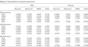
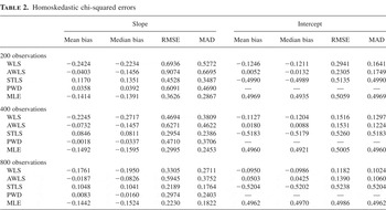
Simulation results for the weighted least squares (WLS) estimator, both with the regressor density known, and with the density estimated from an augmented data set, are reported in Tables 1, 2, and 3. We simulated data from the following model:


The random variables xi,vi were distributed bivariate normal, with correlation of 0.25 and marginals with mean zero and standard deviation of 0.25. The error term ei was distributed independently of vi,xi, either standard normal truncated at −2 and 2, or chi-squared with one degree of freedom, censored at 4, minus its mean. For homoskedastic designs the scale function σ(xi) was set to 1, and for heteroskedastic designs the scale function was set to exp(0.5·xi).
Homoskedastic truncated normal errors

Homoskedastic chi-squared errors

Heteroskedastic truncated normal errors

To simulate the model we first generated a censored data set sequentially until the desired sample size n for the truncated data set was achieved. For the proposed estimator with estimated density function (AWLS in the tables), we estimate the density function from exogeneous variables in the censored data set using kernel methods with a bandwidth of order n*−1/5 to estimate the joint density of vi,xi and a bandwidth of order n*−1/4 for estimating the marginal density of xi, n* denoting the number of observations in the censored data set. The Silverman (1986) rule of thumb was used to calculate the constant, and an Epanechnikov kernel function was used. We set the right truncation point k to be the sample 75th percentile of yi.
For comparison, results are also reported for the symmetrically trimmed least squares (STLS) estimator in Powell (1986), the pairwise difference (PWD) estimator in Honoré and Powell (1994) (this estimator can only identify the slope coefficient, and so no results are reported for its intercept term), and the maximum likelihood estimator (MLE) assuming a homoskedastic normal distribution. The PWD and STLS were computed using linear programming and iterative least squares methods, respectively. The MLE was computed using the BFGS algorithm. The summary statistics reported are mean bias, median bias, root-mean squared error (RMSE), and mean absolute deviation (MAD). Sample sizes of 200, 400, and 800 were simulated with 801 replications.
As the results in Tables 1, 2, and 3 indicate, the proposed WLS estimator performs moderately well at all sample sizes in both the homoskedastic and heteroskedastic designs. The AWLS performs worse for the intercept term, reflecting perhaps the method of bandwidth selection. The MLE performs poorly for all designs as a result of distributional misspecification and/or heteroskedasticity. The STLS poorly estimates the intercept with the chi-squared errors, and PWD performs poorly in the heteroskedastic designs.
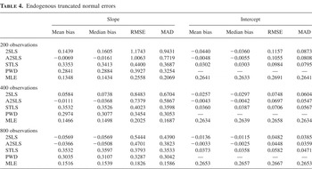
Table 4 reports results for the instrumental variables two-stage least squares (2SLS in the table) estimator. Here we simulated data from the following model:


Endogenous truncated normal errors

To incorporate endogeneity, we simulated a binary variable di that took the value 1 with probability ½ and 0 otherwise. When di was 1, the error term ei was equal to xi, and when di was 0, the error term was drawn from the truncated normal distribution mentioned previously. The instrument zi was independently distributed as uniform between −1 and 1 when di was 1 and equal to xi when di was 0.
Here again we first simulated a censored data set for which the density functions could be estimated and then truncated the data. For implementing the proposed two-stage least squares procedure, we used the same kernel function and bandwidth selection procedure as in the heteroskedastic designs. The constants k and k* needed for this procedure were chosen to be the 25th and 75th percentiles of the dependent variable.
Results using this endogenous model are reported in Table 4 for our two-stage least squares estimator(2SLS) and our estimator using the augmented data set to estimate the density function (A2SLS), and for the STLS, PWD, and MLE. As Table 4 indicates, only the two-stage least squares estimator performs at an acceptable level when the regressor is endogenous. The other estimators, which are inconsistent when the regressors are endogenous, perform very poorly, with biases as high as 35% and not decreasing with the sample size.
Overall, the results of our simulation study indicate that the estimators introduced in this paper perform well in moderately sized samples. The results for the endogenous regressor design are especially encouraging when compared to other estimation procedures.
5. CONCLUSIONS
This paper proposes new estimators for truncated regression models. The estimators are “distribution free” and are robust to general forms of conditional heteroskedasticity, in addition to general forms of measurement error and endogeneity. The proposed estimators converge at the parametric rate and have a limiting normal distribution.
Our limiting distribution theory employs a new variant of asymptotic trimming to deal with boundary bias issues. This is demonstrated for estimation of density weighted averages but should be usefully applicable in general contexts involving two step “plug-in” estimators with a nonparametric first step.
The results in this paper suggest areas for future research. For example, the semiparametric efficiency bound of the models considered needs to be derived under the exclusion restriction we imposed, so that the relative efficiency of our estimators can be computed. Magnac and Maurin (2003) compute the bound for a binary choice model under similar identifying assumptions, and Jacho-Chavez (2005) finds the bound for other similar density weighted estimators. Both find that such estimators are generally semiparametrically efficient.
APPENDIX
The Appendix first develops regularity conditions for a general density weighted closed form estimator and then applies the results to the weighted and two-stage least squares estimators introduced in this paper. Throughout this section ∥·∥ will denote the euclidean norm, i.e., for a matrix A with components {aij},∥A∥ = ([sum ]i,j aij2)1/2; ∥·∥∞ will denote the sup norm over the regressor support.
A.1. Theorem for Density Weighted Estimators.
In this section, we establish the asymptotic properties of a general density weighted estimator. The estimator is defined as a function of the data, a preliminary root-n consistent estimator of a finite-dimensional nuisance parameter (denoted by κ0), and a preliminary estimator of the underlying conditional density function using kernel estimation. Here, we let Ξ0 ∈ Rk denote the parameter of interest in the general setting, defined here as

with ħi,fi* denoting ħ(yi,vi,xi,zi,κ0) and f*(vi|zi), respectively. For any other possible value of the nuisance parameter, κ, we will let ħi(κ) denote ħ(yi,vi,xi,zi,κ). We define the estimator as a sample analogue to the preceding equation:

with

denoting

and

, respectively; τni denotes the trimming function as before, and

denotes an estimator of κ0.
We will assume throughout this section that

has an asymptotically linear representation. Letting the random variables yi,vi and the random vectors zi,xi be as defined previously, we express the representation as

where ψi denotes ψ(yi,xi,vi,zi) and satisfies E [ψi] = 0 and E [∥ψi∥2] < ∞. The estimator of the parameter of interest also involves an estimator of the underlying conditional density function f*(vi|zi). We assume that a kernel estimator is used to estimate this function, and we denote the estimator by

. To define this estimator, we first assume that the vector zi can be partitioned as zi = (zi(c),zi(d)), where zi(c) ∈ RZc is continuously distributed and zi(d) ∈ RZd is discretely distributed. As alluded to in the paper, for identification in the truncated regression model we assume that the population density of the regressors (without truncation) is either known or can be estimated from an alternative or augmented data set. In the latter case, to avoid notational confusion we will distinguish observations from this data set by the superscript * and let n* denote the number of observations for this data set. Regarding relative sample sizes, we will assume limn→∞ n/n* = cp ∈ [0,∞). Furthermore, as the two regressor density functions may be different, we will let rzi,rvzi denote [f (zi)/f*(zi)],[f (vi,zi)/f*(vi,zi)], respectively.
We define the kernel estimator as

where K1 and K2 are “kernel” functions and hn is a bandwidth sequence. Properties of K1, K2, and hn will be detailed in assumptions needed for the main theorems.
Our theorem for the asymptotic properties of

is based on an i.i.d. assumption on the sequences of vectors (yi,vi,xi′,zi′)′ and (vi*,xi*′,zi*′)′ and the following assumptions.
C1. ħi(κ) is continuously differentiable for

, a neighborhood of κ0.
C2.

C3. The function E [ħi(κ)/fi*] is continuous at κ0.
C4. With ∇κ denoting the partial derivative with respect to the nuisance parameter, let Mκ denote E [∇κ(ħi(κ0)/fi*)] and let δni denote the vector

where φnb(·,·) = E [τni rvzi(ħi /fi*)|vi = ·,zi = ·] and φna(·) = E [τni rzi(ħi /fi*)|zi = ·], and let δi denote the mean 0 vector

where φb(·,·) = E [rvzi(ħi /fi*)|vi = ·,zi = ·] and φa(·) = E [rzi(ħi /fi*)|zi = ·]. Then we make the following assumptions.
C4.1.

uniformly in n ∈ N.
C4.2.

.
C5. We let

denote the support of zi, which we assume to be the same for the truncated and untruncated populations. We assume that the support set

is an open, convex subset of RZc and assume that the support of vi, denoted by

, is an open interval in R. Let f*(v,z(c)|z(d)) denote the (population untruncated) conditional (Lebesgue) density of vi,zi(c) given zi(d) and let f*(z(d)) denote the probability mass function of zi(d). Furthermore, let f*(v,z) denote f*(v,z(c)|z(d))·f*(z(d)). Then we make the following assumptions.
C5.1. f*(v,z(c)|z(d)), considered as a function of v,z(c), is p times continuously differentiable, with bounded pth derivatives on

.
C5.2. There exists a constant μ0 > 0 such that for all

, f*(zi(d)) ∉ (0,μ0).
C6. The kernel functions K1(·),K2(·) satisfy the following properties.
C6.1. They are each the product of a common univariate function that integrates to 1, has support [−1,1], and is assumed to be p times continuously differentiable.
C6.2. For two vectors of the same dimension, u,l, we let ul denote the product of each of the components of u raised to the corresponding component of l. Also, for a vector l that has all integer components, we let s(l) denote the sum of its components. The kernel functions are assumed to have the following property:

C7. The functions φna(z) and φnb(v,z) are p times differentiable with bounded pth derivatives, in z(c) and z(c),v, respectively, for all values of z(d) and all n ∈ N.
C8. The trimming function satisfies the following properties.
C8.1. τni is a function of vi,zi, and n only, and 0 ≤ τni ≤ 1 for all n ∈ N.
C8.2. For each

, τni → 1 as n → ∞.
C8.3. For all δ > 0,

, and

, where fvzi* denotes f*(vi,zi).
We now state the theorem for the density weighted closed form estimator.
THEOREM A.1. Suppose Assumptions C1–C8 hold and the bandwidth hn satisfies

and n*1/2+δ/(n*hn2Zc) → 0 for some arbitrarily small δ > 0; then

where

.
Remark A.1. Our assumptions regarding the trimming function τni have particular features that warrant comment. Assumption C8 implicitly makes assumptions regarding where and how quickly the densities fi*,fvzi* approach 0, as was assumed in Sherman (1994). Sherman (1994) provides concrete examples where C8 will be satisfied. Assumption C4 ensures that the bias induced by the trimming function decreases to 0 faster than the parametric rate. For the estimators proposed in this paper, this assumption imposes conditions on the tail behavior of ei,vi,zi and can be satisfied, e.g., if the error term ei has bounded support and vi (strictly) contains the support of ei.
As an alternative to the trimming conditions in C8, which has the drawback of requiring that the researcher know where and how quickly regressor densities go to 0, we propose the following data dependent trimming procedure. This procedure only applies to situations where the regressors have a bounded, “rectangular” support, as opposed to the support assumptions stated at the beginning of Assumption C5. Here we assume that zi(c),vi have compact support that is independent of zi(d).
Specifically, we let zmx denote the Zc-dimensional vector of the maxima in the supports of each of the Zc components of zi(c) and zmn denote the vector of minima. Let vmx,vmn denote the maximum and minimum of vi.
We assume a “rectangular” support of zi(c),vi, providing an alternative condition to C5.
C5′.

, (z(c),v) ∈ [zmn[1],zmx[1]] × [zmn[2],zmx[2]] × … [zmn[Zc],zmx[Zc]] × [vmn,vmx] where superscripts [·] denote components of a vector. Furthermore, the smoothness condition in C5.1 is satisfied on the interior of the rectangular support of zi(c),vi.
Also, before imposing the trimming conditions for these support conditions we slightly modify the smoothness conditions in C7 to account for the rectangular support assumption.
C7′. The functions φna(z) and φnb(v,z) are p times differentiable with bounded pth derivatives on the interior of the (rectangular) support of zi(c),vi.
Turning to the trimming procedure, one form of the infeasible trimming function is the product of Zc + 1 indicator functions:

To define the feasible, data dependent trimming function, let

denote the Zc vector obtained by taking the maximum of each of the components of zi(c) from a sample of n observations. Let

denote the vector of sample minima and analogously denote sample minima and maxima for vi as

, respectively. The feasible trimming function is
C8′.

We now show that for our purposes, the feasible data dependent trimming function is asymptotically equivalent to the infeasible trimming function in density estimation and so we can work with the latter in later proofs.
LEMMA A.1.

Proof. Let An denote

and for an arbitrarily small δ > 0, let Bn denote the event

We have for some arbitrarily small ε > 0

where Bnc denotes the complement of the event Bn. We note that

and the right-hand side goes to 0 by the well-known n-rate of convergence of the extreme estimators under the compact support conditions. Also, we note that

where

We note that by the assumption vi,zi(c) has positive density everywhere on the rectangle, E [Cn] = o(1), and Var(Cn) = o(1), and so P(Cn > ε) → 0, establishing the desired result. █
We now prove the theorem for the density weighted closed form estimator (Theorem A.1). The proof applies to either of the two trimming assumptions and their corresponding support assumptions. For clarity of exposition, we focus on the first set of assumptions and simply note that Assumptions C5′, C7′, and C8′ could be used whenever C5, C7, and C8 are referred to in the proof.
Proof of Theorem A.1. We work with the relationship


We note that the last term is o(n−1/2) by Assumption C4.2. We first focus attention on the first term. The difference in ratios can be linearized, yielding the terms


The remainder term is of order

and is op(n−1/2) by Assumptions C1 and C5–C7 and the conditions on hn (which imply the fourth root consistency with respect to ∥·∥∞ of the kernel density estimator; for the support and trimming conditions C5′ and C8′, see, e.g., Newey and McFadden, 1994, Lem. 8.10; for the conditions C5 and C8, see Sherman, 1994, Cor. 5A). We derive a linear representation for (A.20). A mean value expansion of

around ħi implies that we can express (A.20) as

where ħκi denotes ∇κ ħ(yi,vi,xi,zi,κ*), with κ* denoting an intermediate value. By Assumptions C1–C3 and the root-n consistency of

, we can express

as Mκ + op(1). It thus follows by (A.3) that (A.20) has the following linear representation:

Turning attention to (A.21), we again first replace

with ħi. By the root-n consistency of

and the uniform consistency of the kernel density estimator (for the bounded support case, see Newey and McFadden, 1994; for the support and trimming conditions C5 and C8, see Sherman, 1994), the resulting remainder term is op(n−1/2). We next establish a linear representation for (A.21) with ħi replacing

. As the steps are more involved, we state this as a separate lemma.
LEMMA A.2. Under Assumptions C5–C8, if the bandwidth hn satisfies

and n*1/2+δ/(n*hnZc) → 0 for some arbitrarily small δ > 0, then

Proof. We again work with the identity


where fzi* denotes the true (population) conditional density function of the continuous components of the instrument vector times the probability function of the discrete components and

denotes estimated values. By Assumptions C5 and C6 and the conditions on the bandwidth, by Lemma 8.10 in Newey and McFadden (1994) for the bounded support case, or Sherman (1994) for the unbounded support case, we have that

and

are both op(n*−1/4). It will thus suffice to derive representations for

and

Turning attention to the first of the preceding terms, we let fzi* denote the expected value of the kernel estimator

and work with the decomposition


We note that by the definition of

, (A.29) can be expressed as

To write this in U-statistic form, we will multiply the terms in the double summation by the sequence of numbers vni = I [i ≤ n]. Therefore, the preceding equation can be expressed as

We apply a projection theorem (see, e.g., Powell et al., 1989) to derive a linear representation. Let ζ denote the vector corresponding to observed data, either from the primary or augmented data set, and let χn*(ζi,ζj*) denote the term inside the double summation. We first note that

, which is o(n*) by the conditions on hn. We also note that E*[χn*(ζi,ζj*)|ζi] = 0. It follows by Lemma 3.1 in Powell, Stock, and Stoker (1989) that it will suffice to derive a representation for E [χn*(ζi,ζj*)|ζj*]. We first show that


To show (A.33), we note that

can be written as

A change of variables u = (zj*(c) − zi(c))/hn yields the following integral:

By Assumptions C5–C7 a pth-order Taylor series expansion of φna(zj*(c) − uhn,zj*(d)) around φna(zj*) implies that the preceding integral can be expressed as the sum of φna(zj*) and a remainder term that is of the form

where here pj denotes a vector of nonnegative integers, ∇pjφna(·) denotes partial derivatives of φna(·) with respect to its components, and the order of each partial corresponds to components of pj; the vector u raised to the vector of integers pj denotes the product of the components of u raised to the corresponding component of pj. Therefore, each term in the summation is a scalar, and we sum over all vectors pj where the sum of its components, s(pj), is p. Finally, hn* denotes an intermediate value between 0 and hn. It follows by the dominated convergence theorem and the conditions on hn that

We also note that by the continuity and boundedness of φna(·), an application of the dominated convergence theorem to (A.34) implies that

as hn → 0. Another application of the dominated convergence theorem implies that

as hn → 0. Thus (A.33) follows from Chebyshev's inequality.
To complete the linear representation of E [χn(ζi,ζj*)|ζj*] we show that

Note that

by Assumption C4.2. Note also that ∥E [τni(ħi /fvzi*)(fzi* − fzi*)]∥ is bounded above by

∥ fzi* − fzi*∥∞ = O(hnp) by Sherman (1994) (or, in the bounded support case, by Newey and McFadden, 1994, Lem. 8.9), and E [∥τni(ħi /fvzi*)∥] is bounded for all n by assumption. The desired result follows by the conditions on the bandwidth. To complete the linear representation in (A.26) we show that

First note that ∥E [τni(ħi /fvzi*)(fzi* − fzi*)]∥ is bounded above by

∥ fzi* − fzi*∥∞ = O(hnp) (in the bounded support assumption, by Newey and McFadden, 1994, Lem. 8.9; otherwise, Sherman, 1994), and E [∥τni(ħi /fvzi*)∥] is bounded for all n by assumption. The desired result follows by the conditions on the bandwidth. Therefore, it will suffice to show that

By Chebyshev's inequality it will suffice to establish the preceding relation by showing that

This follows by an application of the dominated convergence theorem and the condition that hn → 0. Using virtually identical arguments, we can show that (A.27) has the following linear representation:

This completes the proof of the lemma. █
Combining all our results we have the following linear representation for the density weighted closed form estimator:

The conclusion of the theorem follows from Assumption C4.2 and an application of the central limit theorem. █
A.2. Truncated Model Estimators.
In this section, we apply the general theorems of the previous sections to derive the limiting distributions of the estimation procedures proposed in the paper. The results are derived under the support, smoothness, and trimming conditions in C5, C7, and C8, but we note that the result also hold under the conditions C5′, C7′, and C8′.
A.2.1. Asymptotics for the Weighted Least Squares Estimator (Proof of Theorem 3.1). Here we derive the limiting distribution of the weighted least squares estimator for the truncated regression model estimator. For notational convenience, here we set ui = xi. We will derive the limiting distribution for the closed form estimators obtained from (3.2). Specifically, here we will let π0 denote (a0,b0′)′ with a0 = 1/α0 and b0 = −β0 /α0. From (3.2) we can define

where here xi = (yi,xi′)′ and

. Note that we have

where

and

.
The proof of limiting distribution theory is based on the following assumptions.
WLS1. 0 < α0 < ∞.
WLS2. The sequences of random vectors (yi,vi,xi) and (vi*,xi*) are i.i.d.
WLS3. The J-dimensional vector xi can be partitioned as (xi(c),xi(d)), where the Jc-dimensional vector xi(c) is continuously distributed and the Jd-dimensional vector xi(d) is discretely distributed. Furthermore, setting zi = xi, assume either the support condition at the beginning of Assumption C5 or the rectangular support assumption in C5′.
WLS4. The error term ei satisfies either E*[ex] = 0 or the stronger condition E*[e|x] = 0.
WLS5. Letting f*(v,x(c)|x(d)) denote the (population untruncated) joint density function of vi,xi(c) conditional on xi(d), we assume that this function is p times continuously differentiable in its arguments v,x(c) with bounded derivatives, for all values of x(d). This smoothness assumption holds over the entire support defined at the beginning of Assumption C5 or on the interior of the rectangular support in C5′.
WLS6.1. The trimming function, here a function of vi,xi,n, satisfies either C8 (if the support condition at the beginning of C5 is satisfied) or C8′ (if condition C5′ is satisfied).
WLS6.2. For the vector ħi = I [0 ≤ yi ≤ k]w(xi)xi(vi − xi′π0), the trimming function satisfies

WLS7. Because we have defined ħi,τni for the estimator at hand, condition C7 is satisfied. Alternatively, C7′ holds if the support and trimming conditions in C5′ and C8′ are satisfied.
WLS8. The matrix H0 ≡ E [wkixixi′] is finite and positive definite, where wki = (I [0 ≤ yi ≤ k]w(xi))/f*(vi|xi).
WLS9. With ħi defined in WLS6.2, δi is defined as in Assumption C4, with zi = xi, zi* = xi*. Defining

, assume ∥Ω∥ < ∞.
We now state the theorem characterizing the limiting distribution of the weighted least squares estimator

of π0 ≡ (a0,b0′)′.
THEOREM A.2. Assume that the bandwidth hn satisfies

, and n*1/2+δ/(n*hnZc) → 0 for some arbitrarily small δ > 0, the kernel function satisfies Assumption C6, and Assumptions WLS1–WLS9 hold. We then have

Proof. Our proof strategy will be to show that the probability limit of the term

is the matrix H0 and use the results from the previous section to derive a linear representation for

. Finally, with the asymptotic distribution theory for π0 ≡ (a0,b0′)′ we can apply the delta method to attain the asymptotic distribution of our estimators of θ0 = (α0,β0′)′.
As a first step note that under the conditions on the bandwidth sequence and the kernel functions (i.e., Assumption WLS3) we can replace kernel density estimates with true values and the remainder term is uniformly (in the support of xi,vi) op(1). (For the bounded support and trimming in C5′ and C8′, see, e.g., Newey and McFadden, 1994, Lem. 8.10; for the support and trimming in C5 and C8, see Sherman, 1994, Cor. 5A.) Thus we are left with the term

Thus by the law of large numbers and Assumptions WLS8 and WLS9 the preceding term converges to H0 ≡ E [wkixixi′]. Note that using (2.10) we can alternatively express H0 as

By assumption WLS8 it follows that

.
Next we apply results from the previous section to derive a linear representation for

First we note that by (2.10) and the conditions on the trimming function behavior (specifically WLS6.2), E [τni wkixi(vi − xi′π0)] = o(n−1/2). Conditions C1–C8 follow immediately from Assumptions WLS1–WLS9. To state the form of the limiting variance matrix of the estimator of π0 we note that ħi /fi* is mean 0 by (2.10), and so δi in WLS9 is mean 0.
Finally, to get the asymptotic variance of the parameters of interest θ0 = (α0,β0) we can simply apply the delta method and pre- and postmultiply the matrix H0−1ΩH0−1 by the Jacobian of transformation. This (J + 1) × (J + 1) matrix, referred to here as Q, is of the form

where 01×J refers to a (1 × J) vector of 0's and IJ×J refers to a (J × J) identity matrix. █
A.2.2. Asymptotics for the Instrumental Variables Estimator (Proofs of Theorems 3.2 and 3.3). The asymptotic properties of the two-stage least squares estimator are based on the following assumptions in addition to the identification assumptions A.1′–A.5′ in the text.
IV1. The random vectors (yi,vi,xi′,zi′)′,(vi*,xi*′,zi*′)′ are i.i.d.
IV2. The Z-dimensional vector zi can be partitioned as (zi(c),zi(d)), where the Zc-dimensional vector zi(c) is continuously distributed and the Zd-dimensional vector zi(d) is discretely distributed. Assume that the support and (population untruncated) density smoothness conditions in Assumption C5 are satisfied or, alternatively, the conditions in C5′.
IV3. E*[∥z∥2] < ∞, E*[∥x∥2] < ∞.
IV4. For the vectors ħ1i = I [0 < yi < k], ħ2i = μ0−22yi I [0 < yi < k], ħ3i = zi(yi* − xi′ β0), define δij,δnij, j = 1,2,3 as in Assumption C4, with ħi = ħji, j = 1,2,3, and assume that C4 is satisfied.
IV5. For j = 1,2,3, the functions τni(rvzi ħji /fi*) satisfy the smoothness of conditional expectation conditions in Assumption C7 or C7′, depending on support conditions.
IV6. The trimming function depends on vi,zi,n and satisfies either Assumption C8 or C8′, depending on support conditions.
We now derive the limiting distribution of the two-stage estimator. Our arguments are based on applying Theorem A.1, and so we will be verifying Assumptions C1–C8. We first derive linear representations for

and

, assuming that α0 > 0. The following lemma characterizes the limiting distribution of the estimator

.
LEMMA A.3. If Assumptions A1′–A5′ and IV1–IV6 hold, and the bandwidth sequence satisfies

, n*1/2+δ/(n*hnZc) → 0 for some arbitrarily small δ > 0, and the kernel function satisfies Assumption C6, then

where μ0 ≡ E [I [0 < yi < k]/fi*] and ψμi is defined as in equation (3.12).
Proof. The result follows directly from Theorem A.1, with ħi = I [0 < yi < k]. █
We can now derive a limiting representation for

.
THEOREM A.3. If Assumptions A1′–A5′ and IV1–IV6 hold, and the bandwidth sequence satisfies

, and n*1/2+δ/(n*hnZc) → 0 for some arbitrarily small δ > 0, and the kernel function satisfies Assumption C6, then

with ψαi defined as in equation (3.11).
Proof. We again apply Theorem A.1. In this case ħi = μ0−22yi I [0 < yi < k], and the plugged-in estimator is

. Note that E [∇μ(ħi /fi*)] = −2μ0−1α0. █
With the established linear representations, we can now derive the limiting distribution of

.
THEOREM A.4. Suppose that Assumptions A1′–A5′ and IV1–IV6 hold and the bandwidth sequence satisfies

, and n*1/2+δ/(n*hnZc) → 0 for some arbitrarily small δ > 0, and the kernel function satisfies Assumption C6. With Δ defined in equation (2.28), and Ωβ as defined right above equation (3.17),

Proof. Define

,

as was done in equations (3.14) and (3.15). Note that we can write

We first note that an application of the law of large numbers and Slutsky's theorem immediately implies that

To complete the proof we apply Theorem A.1 to derive a linear representation for

In this context, ħi = μ0−1zi(yi − viα0)I [0 < yi < k] − zi xi′ β0. The preliminary estimators are

and

. We note that

and

Hence the limiting distribution follows from this linear representation, the convergence of

to Δ, and Slutsky's theorem. █