1. Introduction
Transitioning the gait types is an effective strategy for enabling energetically efficient legged locomotion over a wide range of speeds [Reference Voigt and Hansen51]. The gait type is determined by the specific phase relationship of each leg’s periodic foot touchdown. For instance, horses exhibit trotting and galloping, while bipeds such as humans demonstrate walking and running [Reference Hoyt and Taylor20, Reference Segers, De Smet, Van Caekenberghe, Aerts and De Clercq41]. These animals adaptively adjust their gait in response to changes in locomotion speed [Reference Vasudevan, Patrick and Yang50], thereby optimizing energy efficiency during movement [Reference Diedrich and Warren12, Reference Hoyt and Taylor20]. Understanding the gait transition mechanisms in animals is key to achieving adaptive and energy-efficient legged locomotion in robots.
In the field of bipedal robotics, control methods that incorporate gait transitions have been developed. These methods include using different gait pattern generators based on the target gait type [Reference Hodgins19, Reference Kamioka, Kaneko, Kuroda, Tanaka, Shirokura, Takeda and Yoshiike24] and/or adjusting the trajectory or impedance of the reduced-order model according to locomotion speed [Reference Kobayashi, Sekiyama, Hasegawa, Aoyama and Fukuda26, Reference Smaldone, Scianca, Lanari and Oriolo45]. Such approaches enable robots to change their gait at arbitrary timings and provide energy-efficient gaits optimized for the locomotion speed. However, unlike animals that adaptively transition their gait in response to locomotion speed, these methods only offer a gait transition policy for environments and robots that closely match the assumed model.
Just as a biomechanics study identified the zero moment point as a criterion for stable human walking [Reference Vukobratović and Borovac52], which was subsequently utilized in robot walking controllers [Reference Kajita, Kanehiro, Kaneko, Fujiwara, Harada, Yokoi and Hirukawa23, Reference Takenaka, Matsumoto and Yoshiike49], a method for efficient gait transition should similarly be inspired by an understanding of the mechanisms of gait transition in animals. In the realm of biomechanics, the mechanism behind human gait transitions [Reference Kwon and Park31, Reference Shahbazi, Babuška and Lopes42] is explained using the spring-loaded inverted pendulum (SLIP) model [Reference Blickhan7, Reference Geyer, Seyfarth and Blickhan16]. The efficacy of this model is supported by Geyer et al.’s demonstration that different gaits can be explained using a single model consisting of two SLIP models [Reference Geyer, Seyfarth and Blickhan16]. Mechanistic properties of human locomotion closely resemble those of the SLIP model, as evidenced by gait observation studies in infants learning to walk unassisted [Reference Vasudevan, Patrick and Yang50]. In contrast, the trajectory of the center of gravity (CoG) increasingly resembles that of the inverted pendulum (IP) model as infants develop independent walking abilities [Reference Vasudevan, Patrick and Yang50]. This acquisition of the IP model is closely related to the development of gait without environmental assistance. Moreover, treadmill experiments with varying speeds confirm that gait transitions occur even with passive changes in locomotion speed [Reference Vasudevan, Patrick and Yang50]. Therefore, the gait transition should be explained as a passive transition between the IP and SLIP models in response to environmental changes.
This paper introduces a novel bipedal robot model that behaves as the IP model during walking and the SLIP model during running. It presents a control method enabling the robot to transition between both gaits suitable for passively varying locomotion speeds. This bipedal robot model, capable of describing both walking and running in a unified manner, is developed by focusing on the similarities in leg states and CoG motions between the two gaits. By utilizing this model, a single gait controller is developed to facilitate both walking and running. Hence, simulation verifications reveal that the gait transitions of a robot occur passively, interacting with the environment without explicit gait-type instructions, and can maintain stable walking and running across a wide range of locomotion speeds. Additionally, these passive gait transitions are shown to be energy-efficient for locomotion over various speeds.
The main contributions of this paper are as follows:
-
1. Unified Bipedal Robot Model: We propose a novel bipedal robot model that enables adaptive and passive transitions between walking and running gaits, detailed in Section 3. This model integrates a mechanical model for leg dynamics and a continuous state model that governs gait transitions without explicit state switching, offering a unified framework for walking and running.
-
2. Simple Gait Controller: We develop a single, simple controller based on the bipedal robot model, which can be used for both walking and running, as detailed in Section 4.
-
3. Stability of Locomotion: We demonstrate the stability of the proposed model through dynamic simulations, showing that stable walking and running are maintained across varying speeds, as detailed in Section 5.2.
-
4. Passive Gait Transition: Our controller allows for passive gait transitions driven by environmental interactions and changes in locomotion speed, as detailed in Section 5.3.
-
5. Energy Reduction: By facilitating passive gait transitions, our controller reduces the energy required for locomotion, contributing to more efficient movement across various speeds, as detailed in Section 5.4.
This paper is structured as follows: Section 5.4 introduces relevant studies that underscore the significance of this study and explains the similarities between walking and running. Section 3 proposes a mechanical model that accommodates both walking and running alongside a continuous state model that does not require explicit switching between gait types. Section 4 details the controller developed for the bipedal robot model. The results of the validation are presented and discussed in Section 5. This is followed by a discussion in Section 6, culminating in the conclusions drawn in Section 7.
2. Related work
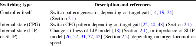
In this section, we review works related to control methods that facilitate gait changes depending on the locomotion speed. First, the section introduces prior studies on control methods for robots capable of gait transitions, emphasizing the importance of passive gait transitions, and the list of related works for gait transition controllers is shown in Table I. Then, the focus shifts to the physical model of gait in biomechanics, detailing the characteristics necessary to commonly represent both walking and running.

2.1. Robot controller modification
In humanoid robotics, the controller system often consists of planners and stabilizers, which include inverse dynamics and kinematics calculations. The planner defines the base trajectory for the center of mass [Reference Kajita, Kanehiro, Kaneko, Fujiwara, Harada, Yokoi and Hirukawa23] and centroidal dynamics [Reference Orin, Goswami and Lee36] and also generates the trajectory for the robot’s footstep or contact points. This planner determines the overall gait behavior. The stabilizer corrects the trajectory by compensating for the error between the actual state and the command from the planner trajectory [Reference Sugihara and Morisawa47] and then outputs the appropriate commands to the robot hardware. Typical control methods based on the linear inverted pendulum (LIP) model employ techniques such as the best COM-ZMP regulator [Reference Sugihara46] and the divergent component of motion [Reference Mesesan, Schuller, Englsberger, Ott and Albu-Schäffer34, Reference Takenaka, Matsumoto and Yoshiike49] to correct model errors and stabilize the trajectory. These values also provide feedback to the planner for additional balance control [Reference Kamioka, Kaneko, Kuroda, Tanaka, Shirokura, Takeda and Yoshiike24]. In this controller scheme, the planner part of the controller defines the desired gait behavior. Therefore, we focus on the planner component in the following sections.
In the study of bipedal walking robots, previous control methods, including gait transitions, involve either switching the controller itself [Reference Egle, Englsberger and Ott14, Reference Hodgins19] and/or altering its internal state [Reference Hanasaki, Tazaki, Nagano and Yokokohji18, Reference Santos and Matos40]. In the switching controller method, specific control rules and pattern generators are prepared for each gait type [Reference Egle, Englsberger and Ott14, Reference Kamioka, Kaneko, Kuroda, Tanaka, Shirokura, Takeda and Yoshiike24]. An auxiliary controller is implemented to facilitate the switching of the primary controller based on operator input or target speeds, thereby explicitly managing gait transitions. In the altering state method, the controllers are often developed based on a reduced-order model with variable states [Reference Hanasaki, Tazaki, Nagano and Yokokohji18] or a central pattern generator [Reference Santos and Matos40]. The former approach enables the CoM to generate vertical motion, which is crucial for both steady-state running and transitions between walking and running, by simply optimizing the stiffness parameter of the liner-inverted pendulum model during each contact phase [Reference Hanasaki, Tazaki, Nagano and Yokokohji18]. The latter approach enables the derivation and adjustment of coordination patterns among the joints in gait motions based on locomotion speed [Reference Khan and Mandava25]. Altering the coordination pattern in response to the target speed enables adjustments in the locomotion speed of the robot [Reference Santos and Matos40], facilitating transitions from walking to running, even though these transitions are discontinuous [Reference Taga, Yamaguchi and Shimizu48].
These methods force the robot to exhibit locomotion patterns that deviate from its inherent dynamics, potentially resulting in energetically inefficient gaits. A gait transition method that leverages the leg dynamics and does not require explicit gait switching is preferable for more efficient locomotion.
2.2. Leg-model modification
Mechanical models of legs have been extensively studied to abstractly represent the dynamics of walking and running [Reference Alexander1, Reference Blickhan7, Reference Geyer, Seyfarth and Blickhan16, Reference McMahon and Cheng33]. Based on the characteristics of the CoG motion in human gait, the IP [Reference Dickinson, Farley, Full, Koehl, Kram and Lehman11] and the SLIP [Reference Blickhan7] models are used for the mechanical models for walking and running, respectively. The SLIP model often elucidates the mechanism of transition between these two gait types [Reference Blickhan7, Reference Ding, Moore and Gan13, Reference Geyer, Seyfarth and Blickhan16]. This approach is primarily attributed to the work of Gayer et al., who demonstrated that both gaits could be explained using a single model comprising two SLIP models [Reference Geyer, Seyfarth and Blickhan16], and thereby the model is extended to a variety of control methods [Reference Davoodi, Mohseni, Seyfarth and Sharbafi10, Reference Jana and Gupta21, Reference Rezazadeh and Hurst39] and has also been used for bipedal robots [Reference Dadashzadeh and Macnab9].
Various control methods that leverage the dynamic properties of mechanical models to enable gait transitions have been developed [Reference Kobayashi, Sekiyama, Hasegawa, Aoyama and Fukuda26, Reference Koo, Trong, Lee, Moon, Koo, Park and Choi27, Reference Kwon and Park31, Reference Owaki, Osuka and Ishiguro37, Reference Shahbazi, Babuška and Lopes42]. Notably, a gait transition in locomotion was effectively demonstrated by using the SLIP model as the mechanical model [Reference Shahbazi, Lopes and Babuska43] and adjusting its stiffness [Reference Shahbazi, Babuška and Lopes42, Reference Shahbazi, Saranlı, Babuška and Lopes44]. However, the SLIP model alone is insufficient to comprehensively represent the human gait, particularly at slower walking speeds. A lower spring constant is required in lower speed ranges to align the oscillation period of the springs with the walking speed. This results in a significant increase in the amplitude of the CoG, and it is difficult to match walking CoG motion. Therefore, explicit impedance control through a model that integrates the viscosity model is necessary [Reference Anand, Seipel and Rietdyk3, Reference Kobayashi, Sekiyama, Hasegawa, Aoyama and Fukuda26, Reference Koo, Trong, Lee, Moon, Koo, Park and Choi27, Reference Kwon and Park31].
These models need appropriate parameters (spring and damper constants) for the specific environment. However, the approach might lead to energetically inefficient gaits under environmental conditions different from those anticipated. In other words, methods that rely solely on the SLIP model require explicit modification of leg parameters to fit the expected environment and also require complex compliant legs with variable stiffness [Reference Ju, Li, Kang, Zhang and Song22, Reference Wang, Zhang, Ma and Jia53]. These methods differ in the gait transition mechanism from humans, who adaptively transition their gait in response to environmental changes [Reference Vasudevan, Patrick and Yang50].
2.3. Biomechanics gait description
In biomechanics studies, distinct mechanical models have been traditionally utilized for walking and running [Reference Alexander1, Reference Blickhan7, Reference McMahon and Cheng33]. According to analyses of human gait, the SLIP model aptly represents running, while the CoG trajectory during walking exhibits similarities to the IP model as individuals acquire independent walking [Reference Vasudevan, Patrick and Yang50]. Furthermore, because gait transitions can also occur due to changes in locomotion speed caused by external factors [Reference Vasudevan, Patrick and Yang50], it is desirable to explain these transitions through passive changes in these different mechanical models.
In studies that use different mechanical models for running and walking, the focus is often on the behavior of the legs during their dominant phases. Running of the single support phase is typically represented by the SLIP model [Reference Blickhan7, Reference Han, Luo, Liu, Zhou and Chen17], while walking of the single support phase is described by the IP model [Reference Alexander1, Reference Bhounsule6]. However, these gaits exhibit distinct behaviors in each phase, even with the same gait type. Running alternates between a flight (
 $\textrm {F}$
) phase and a single support (
 $\textrm {SS}_{\textrm {run}}$
) phase, represented as an inelastic leg (constant acceleration motion) and an elastic leg (SLIP model), respectively [Reference Blickhan7]. Walking involves a single support (
 $\textrm {SS}_{\textrm {walk}}$
) phase and a double support (
 $\textrm {DS}$
) phase, which are described by a rigid leg (IP model) and elastic legs (SLIP model) [Reference Kuo29, Reference Kuo, Donelan and Ruina30]. Despite the similarity in the single support phase (
 $\textrm {SS}_{\textrm {walk}}$
and
 $\textrm {SS}_{\textrm {run}}$
), the difference in the order of contact (
 $\textrm {F}$
 $\rightarrow$
 $\textrm {SS}$
or
 $\textrm {DS}$
 $\rightarrow$
 $\textrm {SS}$
) and the resulting varied state of leg elasticity (SLIP and IP models) make it difficult to explain gait transitions solely through passive behavior of models.
On the other hand, by focusing on CoG motion rather than the behavior of the legs themselves, walking and running show similarities in the shape of their trajectories. The CoG motions in both gaits oscillate upward and downward once in each gait cycle, resembling the motion of a bouncing rubber ball [Reference Cavagna, Saibene and Margaria8]. The CoG trajectory during the
 $\textrm {SS}_{\textrm {run}}$
and
 $\textrm {DS}$
phases is lower convex, while the trajectory is upper convex during the
 $\textrm {F}$
and
 $\textrm {SS}_{\textrm {walk}}$
phases. The legs compress and extend in a manner akin to the elastic leg (SLIP model) during the lower convex trajectory [Reference Kuo29, Reference Kuo, Donelan and Ruina30], and they behave as inelastic legs, not undergoing compression or extension during the upper convex trajectory. Thus, walking and running can be commonly described as alternating between leg elastic states during the lower convex trajectory and inelastic states during the upper convex trajectory.
These variations in the CoG motion are due to its interactions with external forces, including environmental influences. Developing a mechanical model in which the mechanistic properties of the leg passively change in response to external forces can provide a way to explain gait transitions as passive phenomena. This study focuses on the CoG motion and proposes a mechanical model capable of representing both the IP and SLIP models, along with a state model whose state representations do not depend on gait types. Utilizing these models, we aim to develop a bipedal robot model that adaptively transitions between walking and running depending on locomotion speed.

3. Methodology
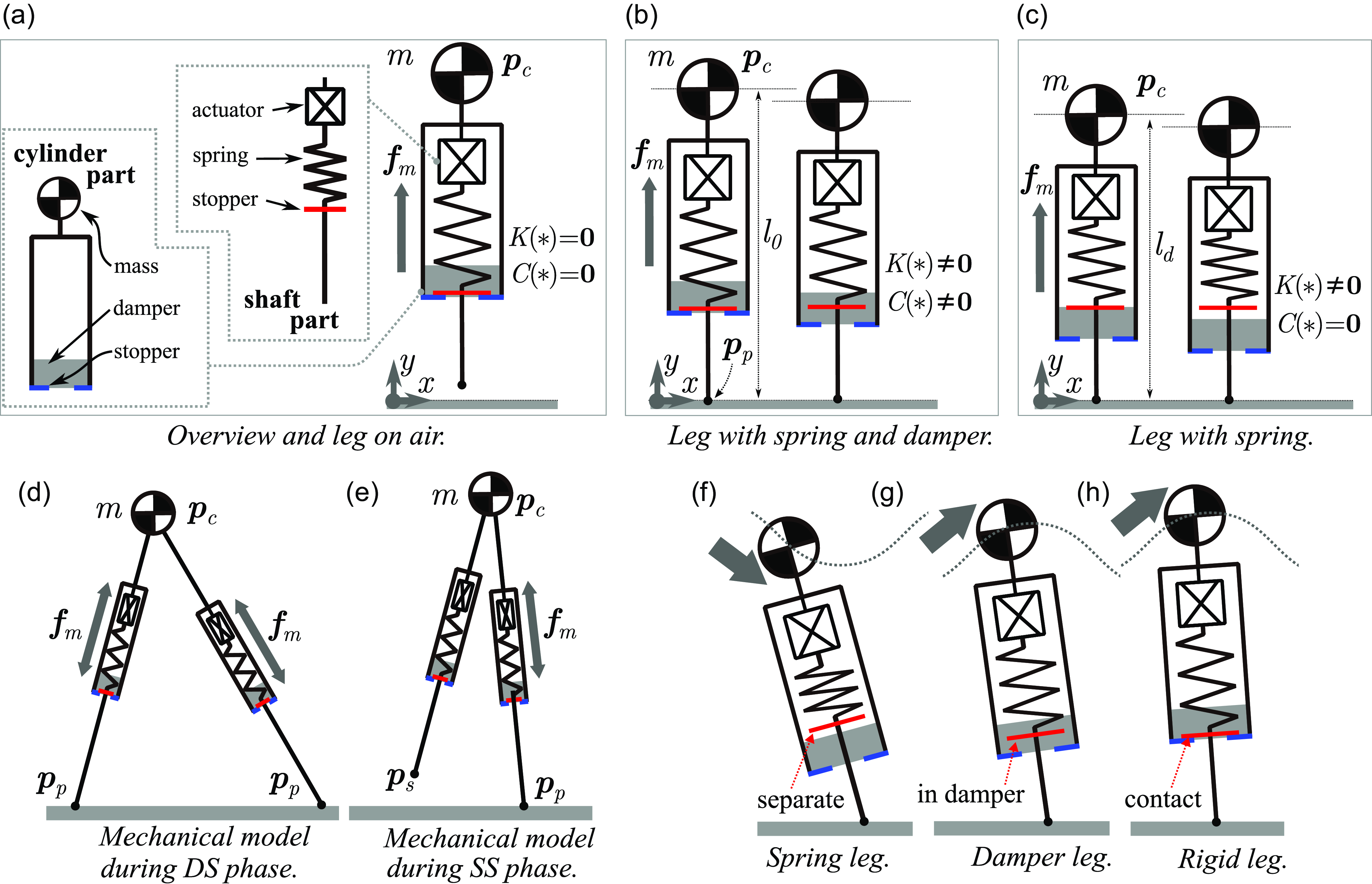
This section presents a biped robot model capable of adaptive gait transitions. The overall structure is shown in Figure 1. The model is constructed from the following two sub-models:
-
(a) Mechanical Model alternates its mechanistic properties between the IP model (inelastic leg) and the SLIP model (elastic leg), depending on the external force and/or ground reaction force,
-
(b) State Model commonly represents the state transitions between walking and running without explicit state switching based on the gait type.
Overview of the spring-loaded inverted pendulum model with a cylinder to replicate the behaviors of both SLIP and IP models. Panel (a) illustrates the structural details with the leg in the air. Panels (a) to (c) show how the spring and damper forces are generated depending on the leg length.
 $K(*)=\boldsymbol {0}$
and
 $K(*) \neq \boldsymbol {0}$
correspond to the lower case and upper case of (2), respectively. Similarly,
 $C(*)=\boldsymbol {0}$
and
 $C(*) \neq \boldsymbol {0}$
represent the lower and upper cases of (3). Panels (d) and (e) indicate how the mechanical model is structured during the DS and SS phases. Panels (f) to (h) display the changes in the mechanical properties of the leg model depending on leg behaviors.

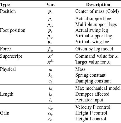
List of variables and parameters. Each position is a two-dimensional vector as
 $\boldsymbol{p}_*=[x_*, y_*]$
.

3.1. Mechanical model
In order to enable passive gait transitions in response to changes in locomotion speed, it is necessary to have a mechanical model for the leg that can switch between inelastic and elastic states depending on external forces and/or ground reaction forces is necessary. Therefore, we propose a novel mechanical model, illustrated in Figure 2, which consists of a cylinder, spring, and damper.
This mechanical model comprises a cylinder part and a shaft part. The lower portion of the cylinder part includes a stopper and a damper part. An actuator, spring, and stopper are connected in series within the shaft part. These two stoppers either make contact or separate. Let the CoM position as
 $ \boldsymbol{p}_{c} = [x_{c}, y_{c}]^T$
, the equation of motion (EoM) for this mechanical model is expressed as follows:
 \begin{align} m\,\ddot{\boldsymbol{p}}_{c} &= \boldsymbol{f}_m +mg[1,0]^T, \\[-10pt] \nonumber \end{align}
 \begin{align} \boldsymbol{f}_m &= K(\boldsymbol{p}_{c}, l_{a}) -C(\dot {\boldsymbol{p}}_{c},\boldsymbol{p}_{c}), \\[6pt] \nonumber \end{align}
where
 $m$
and
 $g$
represent the mass and gravitational acceleration, respectively, and variables and constants frequently mentioned in subsequent sections are listed in Table II. In order to vary the leg properties affected by the stopper, damper, and spring in response to external forces, the spring force
 $ K( \boldsymbol{p}_{c}, l_{a})$
and damper force
 $ C(\dot {\boldsymbol{p}}_{c}, \boldsymbol{p}_{c} )$
are defined in the same manner with Geyer’s SLIP model [Reference Geyer, Seyfarth and Blickhan16] as follows:
 \begin{align} K(\boldsymbol{p}_{c},l_{a}) = \left \{ \begin{array}{l@{\quad}l} k_0 \left ( \frac {l_0 + l_a}{|\hat {\boldsymbol{p}}_{c}|} -1 \right ) \hat {\boldsymbol{p}}_{c}, &\textrm {if}\;\; |\hat {\boldsymbol{p}}_{c}| \lt l_0 \; ;\\[3pt] \boldsymbol {0}, &\textrm {otherwise} \;, \\[3pt] \end{array} \right. \\[-10pt] \nonumber \end{align}
 \begin{align} C(\dot {\boldsymbol{p}}_{c},\boldsymbol{p}_{c}) = \left \{ \begin{array}{l@{\quad}l} c_0\frac {\hat {\boldsymbol{p}}_{c}^T \dot {\boldsymbol{p}}_{c}}{|\hat {\boldsymbol{p}}_{c}|^2} \hat {\boldsymbol{p}}_{c}, &\textrm {if}\;\; l_{d} \lt |\hat {\boldsymbol{p}}_{c}| \lt l_{0} \; ; \\[3pt] \boldsymbol {0}, &\textrm {otherwise} \;, \\[3pt] \end{array} \right . \\[6pt] \nonumber \end{align}
where,
 \begin{align} \hat {\boldsymbol{p}}_{c} = \boldsymbol{p}_{c}-\boldsymbol{p}_{p}. \end{align}
 $ k_0$
and
 $ c_0$
are the spring and damper constants, respectively. Here,
 $ \hat {\boldsymbol{p}}_{c}$
denotes the CoM position with
 $ \boldsymbol{p}_{p}$
as the origin. Define
 $ l_0$
as the natural length of the spring and
 $ l_a$
as the length of the actuator, which indicates the forced displacement from the natural length. When both stoppers are in contact, the leg reaches its maximum length
 $ l_0$
, as illustrated in the left figure of Figure 2(b). As the leg shortens from this maximum length, the stopper initially traverses through the damper region, as shown in the right figure of panel (b), during which both the damper and the spring generate forces. At even shorter lengths, the stopper enters the non-damper region, as illustrated in the right figure of panel (c), during which force is generated only by the spring. Here, let
 $ l_{d}$
be the leg length at the boundary between the damper and non-damper regions. Note that let
 $ \boldsymbol{p}_{p}$
represent the foot contact position with the ground, and its velocity is specified to describe the foot lift-off from the ground as described as
 \begin{align} \dot {\boldsymbol{p}}_{p} = \left \{ \begin{array}{l@{\quad}l} \boldsymbol {0}, &\textrm {if}\;\; |\hat {\boldsymbol{p}}_{c}| \lt l_{0} \; ; \\[3pt] \dot {\boldsymbol{p}}_{c}, &\textrm {otherwise} \; . \\[3pt] \end{array} \right . \end{align}
The EoM from (1a) to (5) represents the mechanical model for a single leg. In order to construct a mechanical model for a biped, the forces
 $f_m$
from both legs need to be added to (1a). Therefore, during the DS phase, each leg is assigned its own leg variables, and both legs independently generate their respective forces
 $f_m$
from (1b), as shown in Figure 2(d). During the SS phase, the single force
 $f_m$
from (1b) is added to (1a), as shown in Figure 2(e).
The mechanistic properties of this model change depending on the external and ground reaction forces applied to the CoM. As depicted in Figure 2(f), when an external force induces a lower convex trajectory of the CoM, the model behaves as an elastic leg (SLIP model) with only the spring action. Conversely, when an external force leads to an upper convex trajectory of the CoM, the model initially behaves as an inelastic leg, predominantly influenced by the damper, as shown in Figure 2(g). Subsequently, the model turns into an inelastic leg (IP model or foot lift-off ) where neither the damper nor the spring has an effect, as illustrated in Figure 2(h). Here, note that in the situation of Figure 2(g), the spring action becomes non-dominant in some cases on the damper parameters. Thus, this mechanical model enables a passive transition between elastic legs (SLIP model) and inelastic legs (IP model, flying), depending on the applied external force.
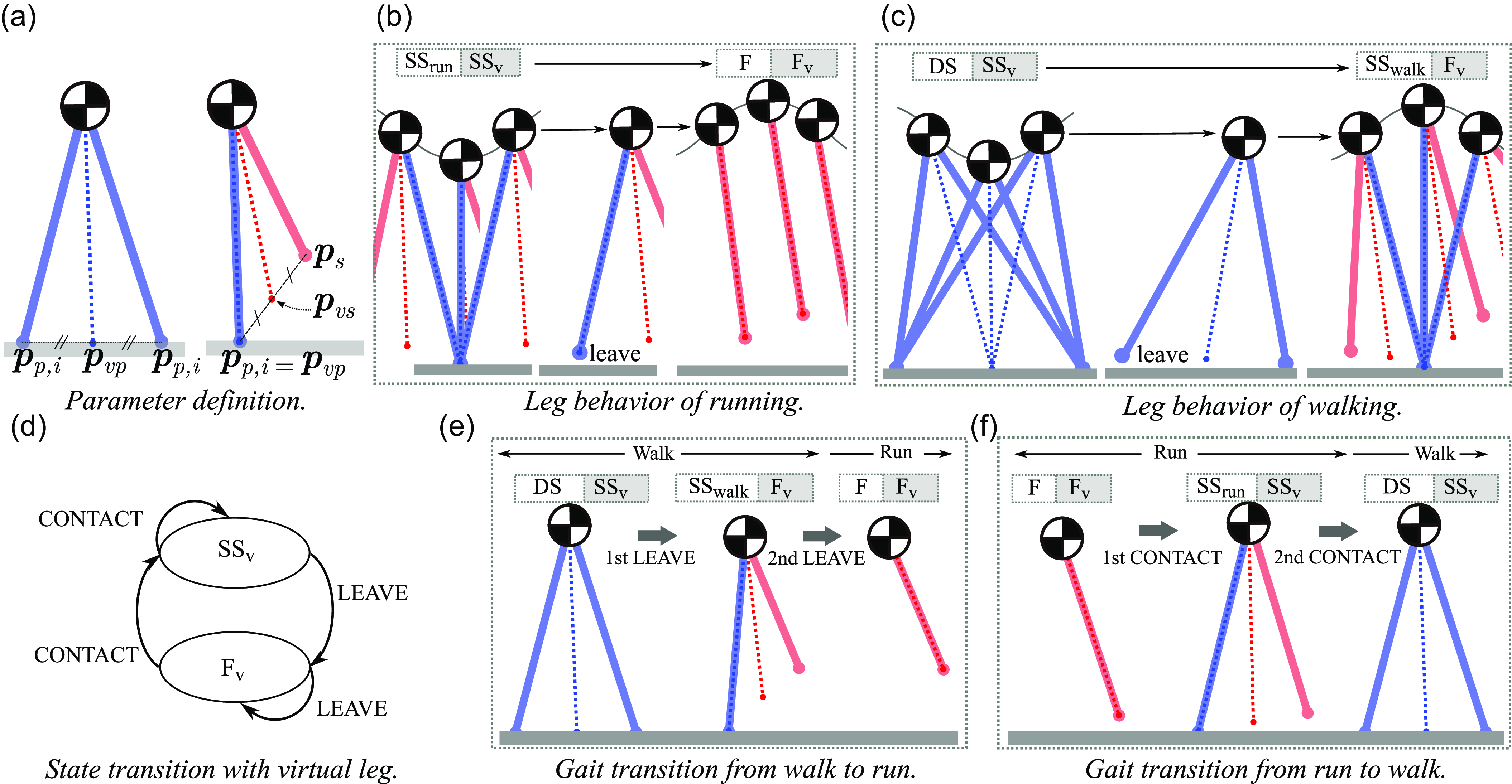
State model for unified gait transition during walking and running. The blue and red lines represent the supporting and swinging legs, respectively. The dashed blue and red lines denote the virtual supporting leg and the virtual swinging leg. The white and gray boxes above the panels indicate the actual gait and virtual leg phases, respectively. Panel (a) illustrates the parameter definitions for the virtual leg description. Panels (b) and (c) depict leg behaviors with virtual legs. Panel (d) presents the state transition diagram. Panels (e) and (f) display leg behaviors during gait transitions.

3.2. State model
A state model that does not differentiate between walking and running is needed for passive adaptation of the gait to suit various environmental conditions, such as external forces, ground reaction forces, and locomotion speed. The state model consists of leg representations and a state machine. In this study, we introduce a state model based on leg representations common to both walking and running, and a state machine developed from these representations.
By introducing virtual leg representations, we develop a unified approach to leg representation applicable to both walking and running. These virtual legs consist of a virtual support leg and a virtual swing leg. As depicted in Figure 3(a), the foot positions of these legs are defined as
 $ \boldsymbol{p}_{vp}$
for the virtual support leg and
 $ \boldsymbol{p}_{vs}$
for the virtual swing leg. The virtual support leg
 $ \boldsymbol{p}_{vp}$
is the midpoint among all actual support legs, while the virtual swing leg
 $ \boldsymbol{p}_{vs}$
is the midpoint between the actual swing leg and
 $ \boldsymbol{p}_{vp}$
. Accordingly, the foot position of the virtual support and swing legs are obtained as follows:
 \begin{align} &\boldsymbol{p}_{vp} = \frac {1}{|L_{p}|}\sum _{i\in L_{p}} \boldsymbol{p}_{{p}, i}, \\[-10pt] \nonumber \end{align}
 \begin{align} &\boldsymbol{p}_{vs} = \frac {1}{2 }(\boldsymbol{p}_{s} +\boldsymbol{p}_{vp} ),\\[6pt] \nonumber \end{align}
where
 $L_{p}$
signifies the set of all actual support legs, and
 $ |L_{p}|$
represents the number of support legs. Therefore, (6) shows the midpoint of all support legs as depicted in Figure 3(a). Define
 $ \boldsymbol{p}_{p,i}$
as an extension variable of the foot position of the actual support leg
 $ \boldsymbol{p}_{p}$
to accommodate multiple legs. These variables are recalculated upon the occurrence of a LEAVE and CONTACT event, which will be defined subsequently, as follows:
Actual Support Leg: when
 $y$
-coordinate of
 $ \boldsymbol{p}_{s}$
is lower equal than zero,
 $ \boldsymbol{p}_{s}$
is reallocated as
 $ \boldsymbol{p}_{p,i}$
Actual Swing Leg: when
 $y$
-coordinate of
 $ \boldsymbol{p}_{p,i}$
is larger equal than zero,
 $ \boldsymbol{p}_{p,i}$
is reallocated as
 $ \boldsymbol{p}_{s}$
.
Using these foot positions of actual support leg
 $ \boldsymbol{p}_{p,i}$
and actual swing leg
 $ \boldsymbol{p}_{s}$
, the virtual legs (6) and (7) are obtained. Note that the controller, which will be detailed in Section 4, adjusts the position of the virtual swing leg
 $ \boldsymbol{p}_{vs}$
, and then this position dictates the position of the actual swing leg,
 $ \boldsymbol{p}_{s}$
.
Utilizing this virtual leg representation allows for the four phases of walking and running (
 $\textrm {DS}$
,
 $\textrm {SS}_{\textrm {run}}$
,
 $\textrm {SS}_{\textrm {walk}}$
, and
 $\textrm {F}$
) to be represented as two phases of virtual legs (
 $\textrm {SS}_{\textrm {v}}$
and
 $\textrm {F}_{\textrm {v}}$
). As shown in Figure 3(b)(c), the virtual support leg during the
 $\textrm {DS}$
and
 $\textrm {SS}_{\textrm {run}}$
phases exhibit behavior similar to that of the
 $\textrm {SS}_{\textrm {run}}$
phase in the running, as indicated by the blue dashed line. Likewise, the virtual swing leg during the
 $\textrm {SS}_{\textrm {walk}}$
and
 $\textrm {F}$
phases mirror the behavior of the
 $\textrm {F}$
phase in the running, as denoted by the red dashed line. Therefore, the
 $\textrm {DS}$
and
 $\textrm {SS}_{\textrm {run}}$
phases enable to be represented as the
 $\textrm {SS}_{\textrm {v}}$
phase of the virtual leg, whereas the
 $\textrm {SS}_{\textrm {walk}}$
and
 $\textrm {F}$
phases can be represented as the
 $\textrm {F}_{\textrm {v}}$
phase of the virtual leg.
Using the virtual legs, the description of walking and running within a single state machine is shown in Figure 3(d). The state machine consists of event conditions and transition rules, while the virtual leg representation provides simple event conditions and transition rules for gait. The event condition is defined to determine whether the virtual leg touchdowns or lift-off from the ground, as follows:
LEAVE: when the foot position of current virtual support is
 $y_{vp}\gt 0$
,
CONTACT: when the foot position of current virtual swing leg is
 $y_{vs}\leq 0$
, and the current CoM velocity is
 $\dot {y}_{c}\leq 0$
.
Here, given that the relationship between the virtual leg and the actual leg is defined through equations (6) and (7), LEAVE corresponds to the lift-off of any actual leg, while CONTACT corresponds to the touchdown of any actual leg. The transition rules are based on the LEAVE and CONTACT events of the virtual legs as follows:
Rule1: when previous event is LEAVE, phase becomes
 $\textrm {F}_{\textrm {v}}$
,
Rule2: when previous event is CONTACT, phase becomes
 $\textrm {SS}_{\textrm {v}}$
.
Only employing this state machine with these simple event conditions and transition rules provides an explanation of the walking and running, including their transition.
First, the leg behaviors of each state transition for walking and running are illustrated in Figure 3(b) and (c), respectively. The walking alternates the
 $\textrm {DS}$
and
 $\textrm {SS}_{\textrm {walk}}$
phases, whereas the running repeats the
 $\textrm {SS}_{\textrm {run}}$
and
 $\textrm {F}$
phases. In the virtual leg representation, both gaits alternate between the
 $\textrm {SS}_{\textrm {v}}$
and
 $\textrm {F}_{\textrm {v}}$
phases. In other words, the same gait pattern is maintained as long as the CONTACT and LEAVE events (or the
 $\textrm {SS}_{\textrm {v}}$
and
 $\textrm {F}_{\textrm {v}}$
phases) occur in alternation. Next, the leg behaviors during gait transitions are shown in Figure 3(e) and (f). Figure 3(e) illustrates the gait transition sequence from walking to running occurs through “
 $\textrm {DS}\rightarrow \textrm {SS}_{\textrm {walk}}\rightarrow \textrm {F}$
.” During these phase transitions, the virtual leg transitions from the
 $\textrm {SS}_{\textrm {v}}$
phase to the
 $\textrm {F}_{\textrm {v}}$
phase following the initial LEAVE event. Subsequently, the position of the virtual support leg is recalculated, as indicated by the blue dashed line in the central diagram, which triggers a second successive LEAVE event. Similarly, two successive CONTACT events from the
 $\textrm {F}_{\textrm {v}}$
phase facilitate the transition from running to walking, as depicted in Figure 3(f). Thus, gait transitions arise when the sequence of alternating CONTACT and LEAVE events (or transitions between the
 $\textrm {SS}_{\textrm {v}}$
and
 $\textrm {F}_{\textrm {v}}$
phases) is discontinued. Furthermore, these transitions are hypothesized to occur when there is excessive energy (in terms of walking speed) relative to the current gait.
The state model does not retain specific information to distinguish between walking and running while enabling it to describe the state transitions for both gait types without distinction of their types. Furthermore, it is assumed that the irregularities in events leading to gait transitions, such as the successive occurrences of CONTACT or LEAVE, arise passively due to changes in the interaction between the robot and the ground depending on the changes in locomotion speed.
The bipedal robot model, comprised of both the mechanical and state models, commonly enables the representation of the robot’s model, regardless of whether the legs function as rigid or spring legs, regardless of whether the current gait type is walking or running. The method has the possibility to autonomously select the gait type depending on the interaction between the environment and the robot. In the subsequent section, a method to control the locomotion speed of this bipedal robot model will be introduced, and this behavior will be verified in dynamics simulations.
4. Implementation of controller
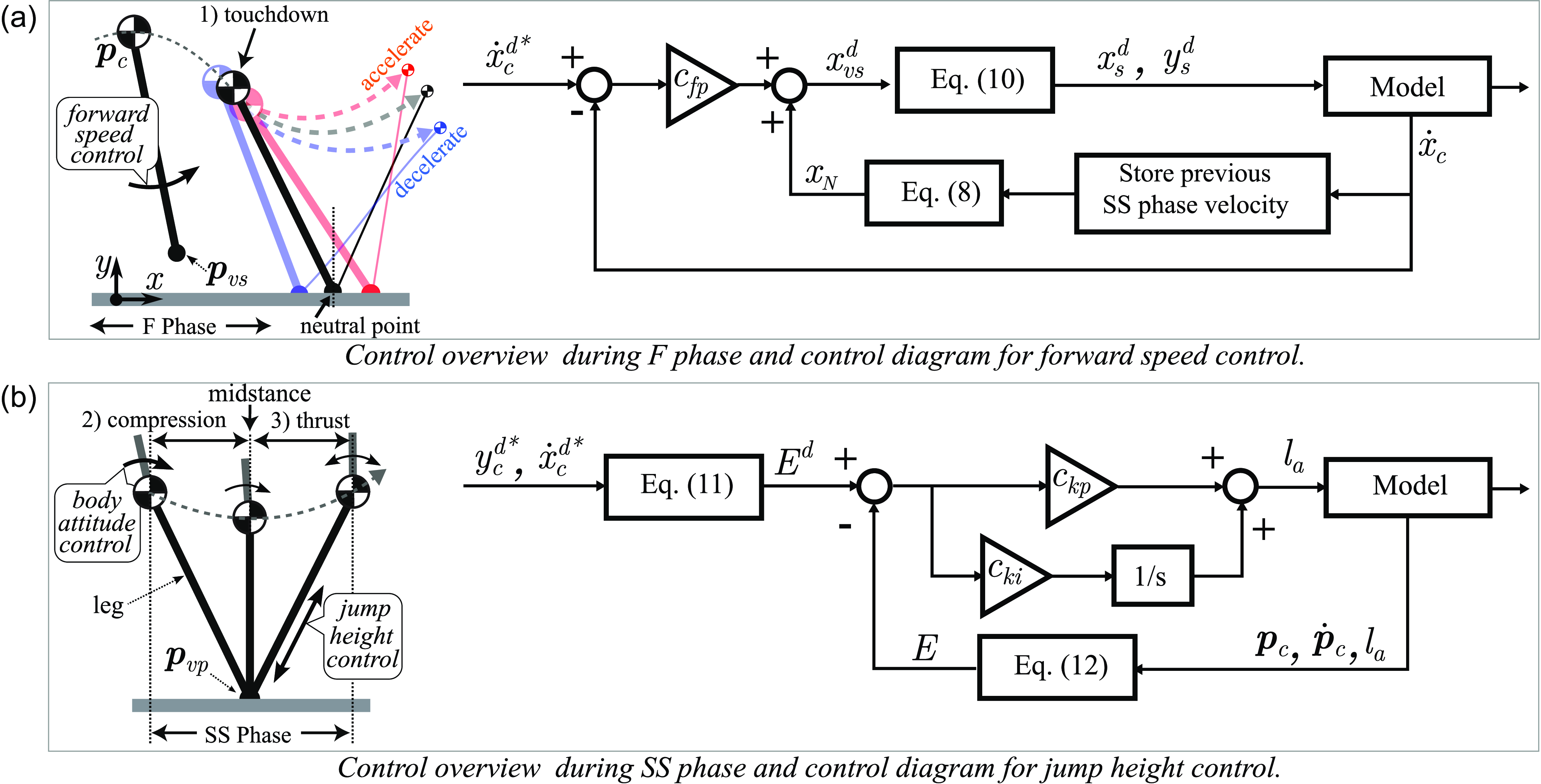
Owing to the similarity in behavior of the proposed virtual legs to running, the control method developed by Raibert et al., often used in running control [Reference Geyer, Saranli, Goswami and Vadakkepat15, Reference Raibert38], is implemented in the controller for our bipedal robot model. The control system treats jump height, forward speed, and body attitude as separate control problems, as illustrated in Figure 4. First, applying leg kick force during the thrust phase adjusts the peak jump height in the
 $\textrm {F}$
phase. This kick force compensates for the energy dissipated through the impact at foot touchdown and the viscoelastic properties of the leg during the compression phase. Second, body attitude control working during the
 $\textrm {SS}$
phase maintains the robot’s upper body posture upright during running. Last, the forward speed is adjusted by foot placement at the touchdown, which is the foot touchdown point at the end of the F phase. The foot touchdown at the neutral point, which is the position where the motion of the support leg is symmetrical during the
 $\textrm {SS}$
phase (indicated by the gray dotted line in the figure), maintains forward speed. When the foot contacts forward or backward from the neutral point, the motion of the support leg becomes asymmetrical (indicated by the red and blue dotted lines in the figure), thereby accelerating or decelerating the forward speed of the robot. Note that this control method is based on the assumption of minimal inertia effects in the legs; this feature is often mirrored in actual robots with designs where the mass is concentrated near the CoM position. Consequently, it is premised that variations in the touchdown point do not affect the behavior during the previous
 $\textrm {F}$
phase.
Phase definition and control diagrams in Raibert controller [Reference Raibert38], which consists of compression, trust phase, and touchdown period. The parameter definitions are in Tables II and III.

Raibert’s control framework allows continuous running with three independently executed control algorithms. In this study, we selectively use the forward speed control and the jump height control from Raibert’s controller to control the running behavior of the virtual leg.
4.1. Forward speed control
The foot touchdown point is determined by adding a positional correction for acceleration or deceleration (p control correction) to the neutral point, which keeps forward speed [Reference Raibert38]. This correction to the foot touchdown point is directly applied to determine the foot point of the virtual swing leg, as detailed in (7). Let the duration and average velocity of the previous SS phase as
 $ T_{PS}$
and
 $ \dot {x}_{PS}$
, respectively [Reference Raibert38], the neutral point is obtained as follows:
 \begin{align} x_{N} = \frac {\dot {x}_{PS} T_{PS}}{2}, \end{align}
where, for simplicity in this study,
 $ \dot {x}_{PS}$
is taken as the velocity
 $ \dot {x}_{\textrm {c}}$
at midstance during the previous
 $\textrm {SS}_{\textrm {v}}$
phase. Note that because the neutral point is dynamically adjusted by the duration (
 $ T_{PS}$
) of the previous SS phase, the neutral point can vary even at the same velocity. The touchdown point of the virtual swing leg touchdown is calculated by adding the neutral point and the p control term, which is determined as follows:
 \begin{align} x^{d}_{vs} = x_{N} + c_{fp}(\dot {x}_{c}^{d*}- \dot {x}_{c}), \end{align}
where
 $ c_{fp}$
is a constant, and
 $d*$
and
 $d$
, denote the target and control command values, respectively. The point of the actual swing leg is obtained by the relationship between (9) and (7) as follows:
 \begin{align} \begin{bmatrix} x^{d}_{s} \\[3pt] y^{d}_{s} \end{bmatrix} = \begin{bmatrix} 2 (x^{d}_{vs} - x_{vp}) + x_{vp} \\[3pt] y_{c} - \sqrt {l_{0}^2 - \left(x^{d}_{s} \right)^2 } \end{bmatrix}, \end{align}
where the position is determined by the target locomotion speed
 $ \dot {x}_{c}^{d*}$
. The control diagram for forward speed control is shown on the right side of Figure 4(a).
4.2. Jump height control
The kick force of the leg is determined by its energy, calculated as the difference between the target energy
 $ E^{d*}$
, based on the desired jump height, and the current energy
 $E$
. Let the target maximum height be defined as
 $ y_{c}^{d*}$
, the target energy
 $ E^{d*}$
is obtained according to:
 \begin{align} E^{d} = mg {y}^{d*}_{c} + \frac {1}{2}m\left (\dot {x}^{d*}_{c}\right )^2. \end{align}
The current energy is obtained as follows:
 \begin{align} E = mgy_{c} + \frac {1}{2}m\dot {\boldsymbol{p}}_{c} \cdot \dot {\boldsymbol{p}}_{c} + \frac {1}{2} \frac {\left ( K(\boldsymbol{p}_{c}, l_{a}) \right ) ^2}{k_0}, \end{align}
where the kick force of our mechanical model results from the forced displacement of the spring
 $ l_a$
. Consequently, the kick force is defined through PI control with the forced displacement
 $ l_a$
as the control input and energy as the control output, as follows:
 \begin{align} l_a = c_{kp}e + c_{ki} \int e dt, \\[-10pt] \nonumber \end{align}
 \begin{align} e = E^{d*} - E, \\[6pt] \nonumber \end{align}
where
 $ c_{kp}$
and
 $ c_{ki}$
represent the p and I gains, respectively. Note that to provide positive energy, the kick force is generated by legs positioned behind the CoM on the
 $x$
-axis. The control diagram for jump height control is shown on the right side of Figure 4(b).
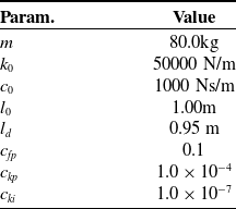
List of parameters for the simulation verifications.

5. Verification
This section shows that the developed bipedal robot model, in conjunction with the previously explained control method, demonstrates the gait transitions of the robot both passively and adaptively. Through dynamic simulations, the stability of the bipedal robot model was demonstrated, and the behavior of the model, along with the dynamics of energy change during the transition, was verified under gradual changes in locomotion speed.
5.1. Setup for simulation
Dynamics simulations were carried out by numerically integrating the EoM from (1a) to (5) using the Euler method. The simulation parameters are specified in Table III. Two simulation scenarios were established. In the first scenario, independent simulations were performed for each target velocity to analyze stability. The target locomotion speeds
 $ \dot {x}^{d*}_{c}$
ranged from
 $0.5$
m/s to
 $3.0$
m/s, with increments of
 $0.01$
m/s between each simulation. Each trial was executed over a duration of
 $50$
seconds at the specified target velocity. The second scenario involved increasing or decreasing the target locomotion speed during a continuous simulation to demonstrate gait transitions. The initial velocity was set at
 $\dot { \boldsymbol{p}_{c} }=[0.5, 0.0]^T$
and gradually increased from
 $0.5$
m/s to
 $3.0$
m/s by
 $0.01$
m/s every
 $2$
seconds. Conversely, another simulation began at
 $\dot { \boldsymbol{p}_{c} }=[3.0, 0.0]^T$
, where the target locomotion speed was decreased from
 $3.0$
m/s to
 $0.5$
m/s. The initial position and target height for both simulations were set to
 $ \boldsymbol{p}_{c} =[0, 1.02]^T$
and
 $ y_{c}^{d*} =0.99$
m, respectively.
5.2. Results of stability analysis
The results of the first scenario are shown in Figure 5. The larger dots represent the result from the first half of the simulation, while the smaller dots represent the results from the second half. These dots illustrate the deviation between the velocity when the CoM reaches peak height position during the previous and current
 $\text {SS}{v}$
phases, a type of Poincaré section. When this deviation converges to zero, it indicates asymptotic stability. Conversely, when the deviation remains within a certain range, it indicates marginal stability. In most of the simulation results, the system exhibits asymptotic stability, as indicated by the convergence of the velocity deviations to zero. However, at around
 $1.3$
m/s and
 $2.0$
m/s, the system does not exhibit asymptotic stability; rather, it demonstrates marginal stability. This is indicated by the clusters of smaller purple dots positioned between the clusters of larger dots, meaning that the velocity deviations remain bounded within a certain range rather than converging to zero. Note that the regions where asymptotic stability does not show correspond to areas where gait transitions occur, which will be explained in detail in the next section. These regions exhibit marginal stability rather than asymptotic stability.tm
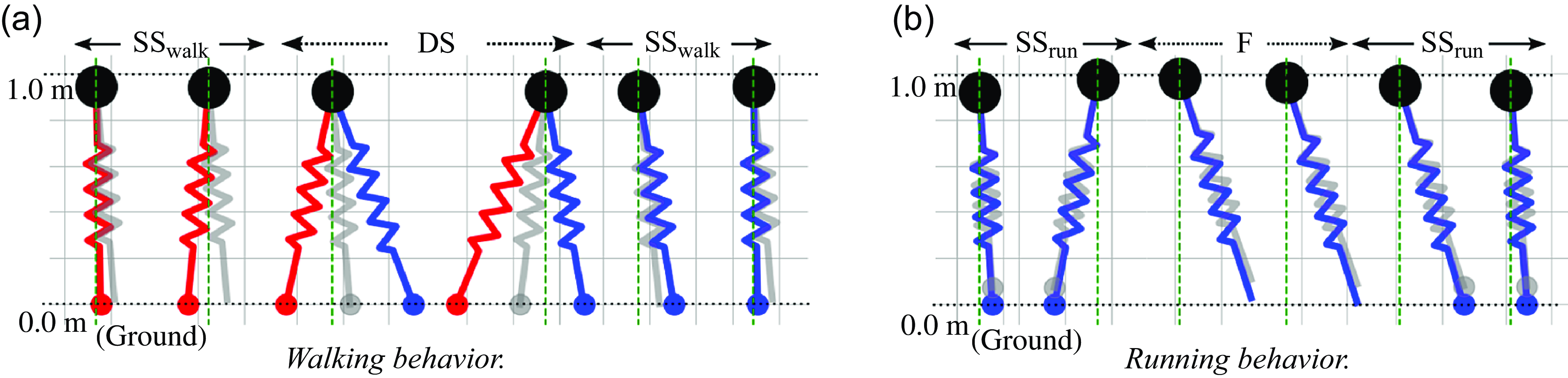
Additionally, in the low-speed range (below 1.8 m/s), the leg behavior corresponds to walking, characterized by alternating
 $\textrm {DS}$
and
 $\textrm {SS}_{\textrm {walk}}$
phases, as shown in Figure 6(a). Conversely, in the high-speed range (above 1.9 m/s), the leg demonstrates running behavior, repeating
 $\textrm {F}$
and
 $\textrm {SS}_{\textrm {run}}$
phases, as shown in Figure 6(b). These results demonstrate that our bipedal robot model can achieve stable locomotion over a wide range of speeds, with the appropriate gait being automatically selected based on the speed.
Result of the Poincaré section for velocity deviations for each individual target velocity. Each dot represents the velocity deviation between the current and previous phases, where the speed is measured when the CoM reaches peak height position.

Leg behavior in simulation. The red and blue legs show the actual legs, which are the left and right feet. The gray shows the virtual legs. While the legs come in contact with the ground, round markers at the tip of the legs are shown. Panel (a) shows a walking motion. Panel (b) shows a running motion.

Phase diagrams during the target speed are changed discontinuously during a continuous simulation. The target speed of panel (a) is changed from
 $0.5$
m/s to
 $3.0$
m/s every
 $0.01$
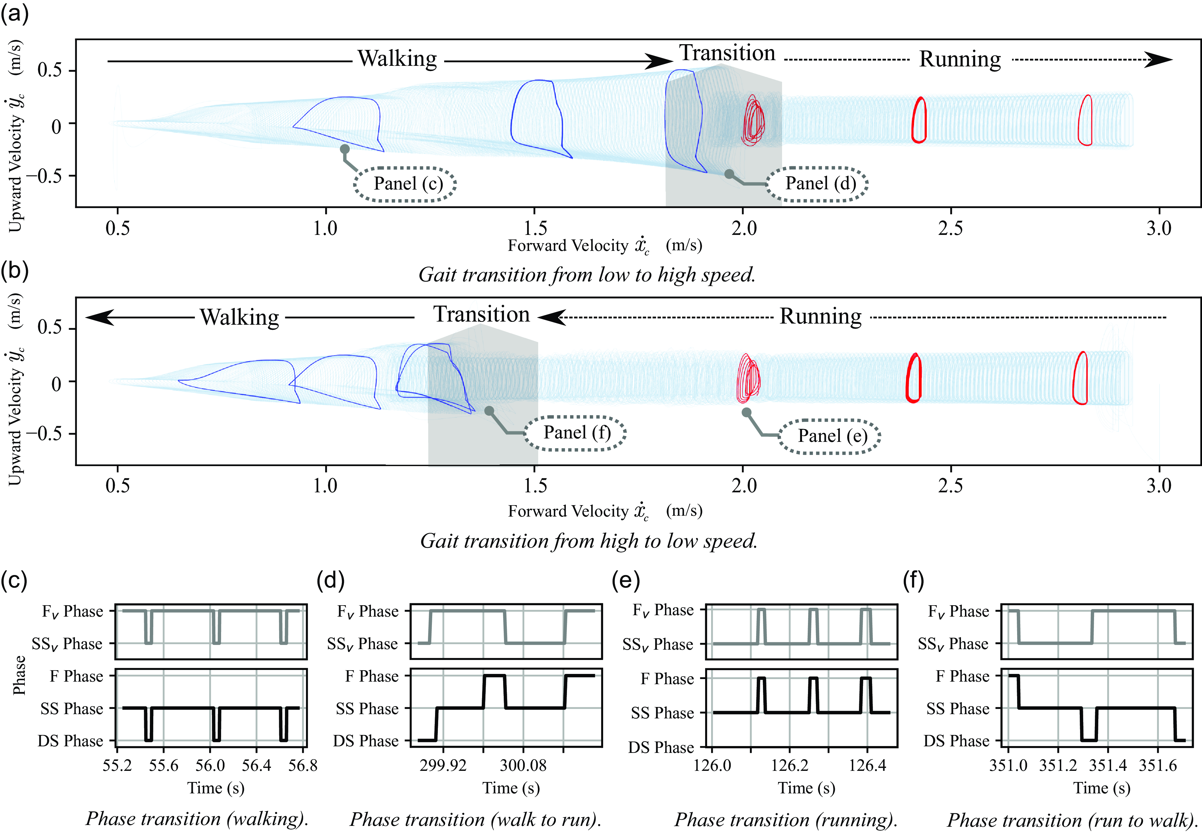
m/s, and it of panel (b) is the reverse. Although the result of decreasing and increasing speed has hysteresis, this graph shows stable motion in any speed range. Panels (c) to (f) show the actual phase transitions for the virtual leg and the actual leg, with their timings illustrated in panels (a) and (b), respectively.

5.3. Results of gait transition behavior
The results of the second scenario are shown in Figure 7. Panels (a) and (b) show simulation results that depict changes in the CoM velocity to verify passive gait transitions. The thin blue line of the figure is the CoM velocity
 $\dot { \boldsymbol{p}_{c} }$
. The bold blue line illustrates
 $\dot { \boldsymbol{p}_{c} }$
at certain target speeds; the bold blue line represents walking, while the bold red line represents running. Panels (c) to (f) show the phase transitions for both the virtual and actual legs to provide insight into how the gait transitions occur. The gray lines represent the phases of the virtual legs, while the black lines depict the resulting phases of the actual legs.
First, the walking pattern is depicted as the bold blue line in Figure 7, which shows trapezoidal limit cycle trajectories. During walking, the phases of the virtual legs alternate between the
 $\textrm {SS}_{\textrm {v}}$
and
 $\textrm {F}_{\textrm {v}}$
phases, while the phases of the actual legs alternate between the
 $\textrm {DS}$
and
 $\textrm {SS}_{\textrm {walk}}$
phases, as shown in Figure 7(c). This pattern aligns with the explanation provided in Figure 3(c).
Second, the running pattern is depicted as the bold red line in Figure 7, which shows a semicircular limit cycle trajectory. During running, the phases of the virtual legs alternate between the
 $\textrm {F}_{\textrm {v}}$
and
 $\textrm {SS}_{\textrm {v}}$
phases, while the phases of the actual legs alternate between the
 $\textrm {F}$
and
 $\textrm {SS}_{\textrm {run}}$
phases, as shown in Figure 7(e). This pattern also aligns with the explanation provided in Figure 3(b).
Third, the walk-to-run transition behavior is shown in the delineated gray region of Figure 7(a), with phase transitions illustrated in Figure 7(d). At the beginning of the gait transition, the phase of the virtual legs transitions from
 $\textrm {SS}_{\textrm {v}}$
to
 $\textrm {F}_{\textrm {v}}$
, while the phase of the actual legs transitions from
 $\textrm {DS}$
to
 $\textrm {SS}_{\textrm {walk}}$
. At that moment, the virtual stance leg is recalculated by (6) and is placed in the same position as the current actual stance leg. Next, when both the virtual and actual stance legs leave the ground, the phase of the actual legs transitions from
 $\textrm {SS}_{\textrm {walk}}$
to
 $\textrm {F}$
, while the phase of the virtual legs remains in the
 $\textrm {F}_{\textrm {v}}$
phase. Consequently, the gait phase transitions to running. This pattern also aligns with the explanation provided in Figure 3(e).
Lastly, the run-to-walk transition behavior is shown in the delineated gray region of Figure 7(b), with phase transitions illustrated in Figure 7(f). At the beginning of the gait transition, the phase of the virtual legs transitions from
 $\textrm {F}_{\textrm {v}}$
to
 $\textrm {SS}_{\textrm {v}}$
, while the phase of the actual legs transitions from
 $\textrm {F}$
to
 $\textrm {SS}_{\textrm {run}}$
. At that moment, the virtual swing leg is recalculated by (7), while the actual swing leg is redefined by (10). Next, when the actual swing leg contacts the ground, the phase of the actual legs transitions from
 $\textrm {SS}_{\textrm {run}}$
to
 $\textrm {DS}$
, while the phase of virtual legs remains in the
 $\textrm {SS}_{\textrm {v}}$
phase. Consequently, the gait phase transitions to walking. This pattern also aligns with the explanation provided in Figure 3(d).
These graphs show hysteresis existing in the speeds at which gait transitions occur. These regions, where the robot exhibits marginal rather than asymptotic stability in the stability analysis (as shown in Figure 5), are closer to the areas where gait transitions occur, as indicated in Figure 6. During the speed increase from low to high depicted in Figure 6(a), the gait transition is observed at approximately
 $2.0$
m/s. Conversely, during the speed decrease from high to low, as shown in Figure 6(b), the gait transition occurs at around
 $1.4$
m/s. While these results indicate the presence of hysteresis and some regions of non-asymptotic stability, the system in all regions exhibits either asymptotic or marginal stability. These results indicate that the gait transitions of the robot occur passively, triggered by the interaction between the robot and the environment in response to changes in locomotion speed, and that a stable gait can be maintained across a broad spectrum of speeds.
5.4. Result of input energy
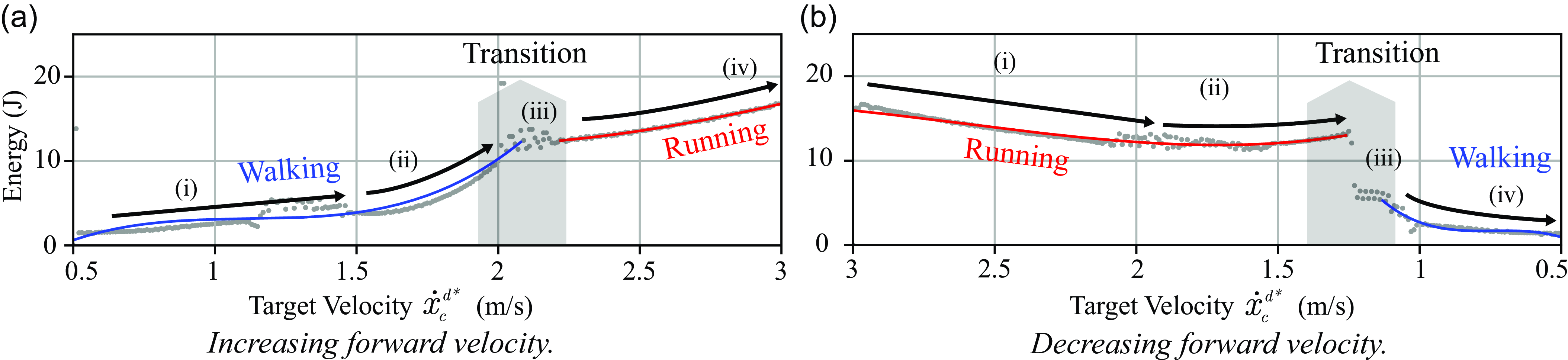
To verify that an adaptively efficient gait is selected, the energy consumed during the simulations of the second scenario was calculated, and the results are shown in Figure 8. The total energy input from the kick force (jump height control) at each target speed is plotted as gray dots. The cubic curve approximation of these points is represented by bold lines (red and blue), with the blue line indicating the walking and the red line indicating the running state.
The input energy for the transition from low to high speed is depicted in Figure 8(a), with the transition phases marked as (i)
 $\sim$
(iv). Initially, in (i), the robot begins walking, with input energy monotonically increasing alongside locomotion speed. Upon further velocity increase, (ii) exhibits a sharp escalation in input energy, yet the robot continues to walk. Continuing to increase the speed led to a significant change in the rate of energy increase in (iii), transitioning to a running gait. Subsequently, in (iv), the energy monotonically increased at a rate smaller than in (ii). These changes of energy are also shown in the transition from high to low speeds, shown in panel (b), through the speed range for (iii).
Hence, as the target speed increases (decreases), the energy consumption for gait correspondingly increases (decreases). Fundamentally, these results showed gradual energy changes, as illustrated in phases (i) and (iv) in Figure 8. On the other hand, as the locomotion speed closes to the speed range for gait transition, indicated by the gray area, a significant amount of energy is needed, exceeding these gradual changes (i) and (iv). In other words, the results indicate that an excess of energy is required before the gait transition occurs, and the transitioning gait makes the robot reduce the needed energy.
In summary, our proposed bipedal robot model has demonstrated passive gait transitions through modifications in locomotion speed. Furthermore, it has been confirmed that the process of gait transition contributes to a reduction in the energy necessary for locomotion across the respective speed range, thereby enhancing energy efficiency.
Change in energy as a function of target velocity. Panel (a) shows the change from low to high speed, and panel (b) shows the reverse.

6. Discussion
The results indicated that our method passively transitioned from walking to running gait and vice versa using the same stiffness (mechanical model), a single state transition rule, and a single controller without explicit controller switching. Similar gait transition controllers based on the spring-mass model, on the other hand, explicitly change the impedance of a damper-added SLIP model [Reference Kobayashi, Sekiyama, Hasegawa, Aoyama and Fukuda26] or discontinuously adjust the stiffness of the SLIP model, even though they use a unified mechanical model for both walking and running [Reference Shahbazi, Babuška and Lopes42]. These controllers, which explicitly change internal states [Reference Kobayashi, Sekiyama, Hasegawa, Aoyama and Fukuda26, Reference Shahbazi, Babuška and Lopes42], require a significant increase in energy during the transition from walking to running. In contrast, our proposed controller reduced energy consumption or the rate of change in required energy after gait transitions compared to before the transitions. Therefore, our method automatically selected the energy-efficient gait, which may allow humanoid robots to achieve more efficient motion behavior.
Our mechanical model, to account for the relationship between leg length and viscoelasticity, exhibits qualitatively similar characteristics to the human leg. The human leg is a linkage mechanism that reaches a singularity at the end of its extension and is driven by muscles with viscoelastic elements. In this structure, the change rate of the knee joint angle in relation to leg length varies, resulting in different mechanical behaviors depending on its length. Consequently, viscous forces dominate when the leg is extended, yielding a rigid leg akin to the IP model. In contrast, elastic forces prevail when the leg is contracted, resulting in a compliant leg akin to the SLIP model. Similarly, our model transitions between elasticity and inelasticity based on leg length, suggesting that even with a linkage structure similar to humans, it can naturally exhibit both the IP model for walking and the SLIP model for running, depending on the locomotion speed.
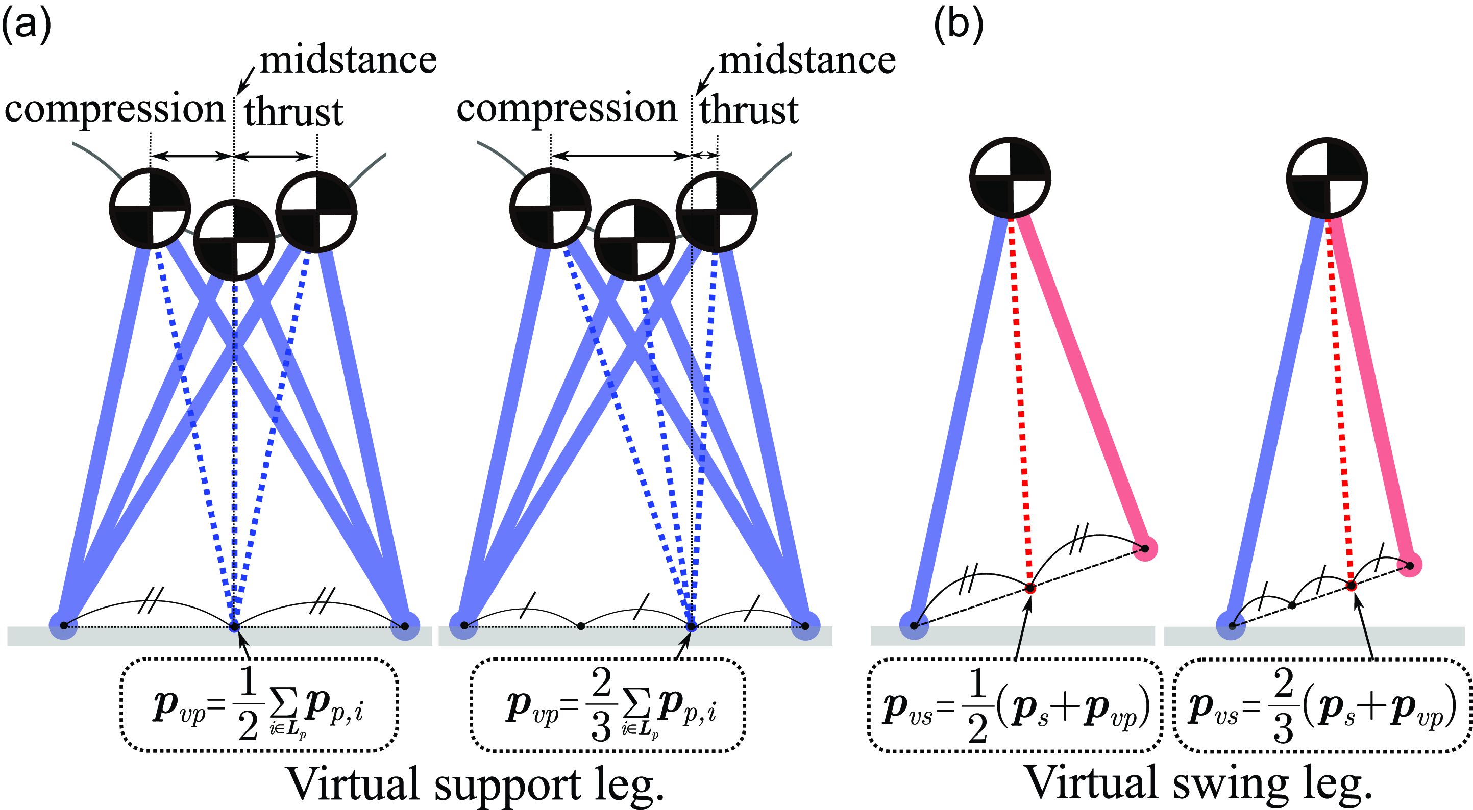
Our state model employs the virtual legs to commonly represent running and walking. The behavior of the virtual legs changes depending on the coefficients applied to (6) and (7) as shown in Figure 9. As shown in panel (a), modifying the coefficient of (6) alters the midstance posture and the timing of the kick (thrust phase). Similarly, modifying the coefficient of (7), as illustrated in panel (b), changes the point of the swing leg and, consequently, the stride length at touchdown. The model assumes uniform physical parameters for all actual legs, with the trajectories of the support legs being symmetrical around the midstance position at a steady state. In animals, the stiffness and natural leg length can differ between legs [Reference Ma, Zhu, Zhang, Xiao, Liu, Leng, Yu and Fu32], potentially resulting in asymmetrical supporting leg motion. By adjusting the parameters of the virtual legs, it may be possible to achieve control that accommodates these asymmetrical support leg trajectories.

An assumed potential function that explains the hysteresis in the gait transition (modified from [Reference Aoi, Katayama, Fujiki, Tomita, Funato, Yamashita, Senda and Tsuchiya4, Reference Diedrich and Warren12]).

The results of two simulations representing gait transitions indicate that transitions occur at different speeds. The velocity range for gait transitions during deceleration is smaller than during acceleration. Hence, the potential function representing the stability of the locomotion in this simulation could be visualized as shown in Figure 10. In both low and high-speed ranges, only a single attractor is present. When the locomotion converges to one of these attractors, the gait type becomes running at high speeds or walking at low speeds. On the other hand, in the mid-speed range, two attractors exist, leading to hysteresis within the speed range of gait transition. Depending on the direction of the speed change, the same speed can result in running or walking. This phenomenon also occurs in the gait transitions of animals and aligns with numerous studies [Reference Aoi, Katayama, Fujiki, Tomita, Funato, Yamashita, Senda and Tsuchiya4, Reference Aoi, Yamashita, Ichikawa and Tsuchiya5, Reference Diedrich and Warren12] showing that gait transitions occur at different speeds based on the direction of speed change.
7. Conclusion
In this study, we aimed to develop a control method that enables passive and adaptive gait transitions by merely setting a target speed without explicitly instructing the gait types. To this end, a bipedal robot model was developed, focusing on the dynamics of the human leg during walking and running. The model consists of a mechanical model that transitions between elastic legs (SLIP model) and inelastic legs (IP model) based on external force and a state model with virtual leg representations that commonly express walking and running. A simple controller, independent of the gait state, was developed using our bipedal robot model. As a result, dynamics simulation showed stable walking and running, demonstrating passive gait transitions in response to locomotion speed. Moreover, the results indicated that the robot adaptively selects a gait suitable for energy efficiency and locomotion speed. These two results indicate that our proposed bipedal robot model possesses the characteristics of both the IP and SLIP models and can adaptively transit an energy-efficient gait depending on the speed. Furthermore, these results support the universal biological insight into the dependency of gait transitions on speed, which occur dependent on speed and lead to efficient locomotion [Reference Alexander2, Reference Diedrich and Warren12, Reference Kram, Domingo and Ferris28, Reference Minetti35]. For future study, a three-dimensional extension with a model incorporating both the torso and legs is necessary for application to real robots. This will contribute to research on adaptive and efficient control of bipedal locomotion robots.
Author contributions
HS and SI conceived and designed the study. HS conducted and developed a controller, simulator, data gathering, and analyses. HS and SI wrote the article.
Financial support
This research received no specific grant from any funding agency, commercial, or not-for-profit sectors.
Competing interests
The authors declare no conflicts of interest exist.
Ethical approval
None.
Supplementary material
The supplementary material for this article can be found at https://doi.org/10.1017/S0263574724002248.