3.1. Linear model predictions

Dispersion relations obtained using the 3-D vTG framework subject to the nonlinear simulation base profiles are presented in figure 2. Solutions are obtained for four spanwise wavenumbers $k_z$ over a wide range of streamwise wavenumbers $k_x$, and visualised using the log-scaled growth rate, $\sigma$. Note that all modes are stable ($\sigma < 0$), and while the logarithmic scaling on the growth rate of figure 2 emphasises the differences in growth rates between the dominant modes, both are reasonably close to marginally stable, particularly when $k_x$ and $k_z$ are small.

Figure 2.

Dispersion relation predictions for 3-D vTG solutions, visualised using the growth rate $\sigma$, with background profiles and parameters taken from simulation data. Solutions obtained with spanwise wavenumbers of (a) $k_z = 0$, (b) $k_z = 2$, (c) $k_z = 8$ and (d) $k_z = 40$. Dash-dotted lines are marked in each panel representing the dominant modes: FW and BW. Horizontal lines are as per figure 1(c).

Solving the 3-D vTG equations with increasing values of $k_z$ (figure 2) leads to a significant deviation from the $k_z=0$ solutions, particularly for the forward-propagating modes. As $k_z$ increases, the two dominant modes migrate towards the idealised dispersion relation, $\omega = U_{max} k_x \pm N_{max}$. This limiting behaviour is explained when investigating idealised systems in § 3.2. Interestingly the forward modes maintain their near-zero (marginally stable) growth rates as $k_z$ increases, while the backward modes weaken.

The solution with $k_z=0$ (figure 2a) is a reproduction of the 2-D vTG predictions adopted by Lloyd et al. (Reference Lloyd, Dorrell and Caulfield2022). When compared against the 2-D spanwise-averaged spectra of figure 1 it is clear that while the form of the BW dispersion relation is well predicted, that of the FW is not. This poor prediction is entirely due to the spanwise-averaging performed on the spectra. To directly compare with nonlinear simulations we have calculated 3-D spectra $E_{b b}^{3D}(k_x,k_z,\omega )$ at $y=1$. To improve convergence, the temporal Hamming window has been halved to 2048 snapshots with respect to the 2-D spectra calculations of figure 1. Spectra are shown in figure 3 for the same four $k_z$ values as in figure 2 and directly compared against the dominant vTG modes, marked by the dash-dotted lines. The 3-D energy spectra indicate excellent agreement between the simulations and the vTG solutions, with both the FWs and BWs migrating towards $\omega = U_{max} k_x \pm N_{max}$ as $k_z$ increases. In addition, the FWs are detected over the full frequency axis limits in figure 3, unlike figure 1 where spectral energies decay significantly as $k_x$ increases. The backward waves are largely 2-D, demonstrated by their substantial decrease in energy content as $k_z$ increases. In contrast, the spectral energy content of the forward waves is considerably less sensitive to $k_z$, even for $k_z=8$ (figure 3c). In agreement with vTG solutions, the spectral energy of the forward waves grows in amplitude relative to that of the backward waves as $k_z$ increases; while they never dominate over the backward waves, they do become an important feature.

Figure 3.

The 3-D energy spectra of buoyancy perturbations at $y=1$, as a function of streamwise wavenumber $k_x$, spanwise wavenumber $k_z$ and temporal frequency $\omega$. Spectra obtained for spanwise wavenumbers of (a) $k_z = 0$, (b) $k_z = 2$, (c) $k_z = 8$ and (d) $k_z = 40$. Dash-dotted lines represent the dominant modes obtained from the vTG solutions of figure 2. Lines are as per figure 1(c).

Clearly, spanwise structure is a vital component for both the nonlinear simulations and the vTG solutions; accounting for $k_z$ leads to excellent agreement between linear stability analysis and fully nonlinear simulations, for both sets of waves. When neglecting spanwise information by averaging in $z$ (as per figure 1) the FWs are smeared out due to their presence over a wider range of $k_z$, and the dependence of their dispersion relation on $k_z$.

While fixing $k_z$ for each panel of figures 2 and 3 is a natural choice for the nonlinear simulation data, interpretation of the dispersion relations is difficult due to the changing angle of obliquity $\theta$ as $k_x$ increases, where $\tan \theta = k_z / k_x$ or $\cos \theta = k_x / \tilde {k}$. At low $k_x$ the modes of figures 2 and 3 are more oblique (higher $\theta$) than at high $k_x$. To resolve this we present the dispersion relations for the vTG solutions with constant angles of obliquity in figure 4: $\tan \theta = 0$, 1, 2 and 4, as a function of the wavenumber magnitude, $\tilde {k}$. First note that the dispersion relations of all modes intersect the origin with $\tilde {k}=0$ and $\omega = 0$, unlike figures 2 and 3. In addition, $\theta$ has a smaller influence on the dispersion relation than $\tilde {k}$; its influence is restricted primarily to the BW in the region $\tilde {k} \lesssim 25$. The (negative) intrinsic frequency of the BW reduces as $\tilde {k}$ increases from zero until it reaches its maximum growth rate, at which point its intrinsic frequency starts increasing with increasing $\tilde {k}$. This turning point is not present in the FW dispersion relation. As we show in § 3.2, the turning point in the BW dispersion relation at low $\tilde {k}$ is strongly dependent on the background shear.

Figure 4.

Dispersion relation predictions for vTG solutions, visualised using the growth rate $\sigma$, with background profiles and parameters taken from simulation data. Solutions obtained with increasing angles of obliquity: (a) $\tan \theta = 0$, (b) $\tan \theta = 1$, (c) $\tan \theta = 2$ and (d) $\tan \theta = 4$. Lines are as per figure 2.

At high $\tilde {k}$ the BWs and FWs very clearly tend towards $\omega = U_{max} k_x \pm N_{max}$, demonstrating that the wavenumber magnitude $\tilde {k}$ is the key control on limiting behaviour. As $\tilde {k}$ and $\theta$ increase, the growth rate of the FW monotonically decreases. In contrast, the BW has a maximum growth rate at $\tilde {k} \approx 4$ which decays as $\tilde {k}$ increases further. Both the BW and FW become more stable as $\tilde {k}$ increases, and are therefore likely to quickly decay when compared with the near marginally stable modes at low $\tilde {k}$. These features are consistent with the simulation spectra of figure 3. A clear discrepancy between the linear stability analysis and the simulations is the dominance of the FW over the BW in the linear solutions; this is revisited in § 3.4.

The vertical structure of the dominant modes is assessed by calculating $E_{v v}^{2D}(k_x,y,\omega )$ and $E_{b b}^{2D}(k_x,y,\omega )$ using $z$-normal snapshots. These spectra are reported as a function of frequency $\omega$ and height $y$ for a given wavenumber $k_x$ in figure 5, and compared against the vertically varying dispersion relations $U k_x$ and $U k_x \pm N$. It is important to note, however, that spanwise structure cannot be assessed using the $z$-normal slice data. Nevertheless, the vertical dependence of $E^{2D}$ does reveal some additional insights. The BWs appear to have a near-constant frequency for a given $k_x$, with its main spectral energy bound by the channel core $0.8 < y < 1.2$ before reducing in magnitude in the outer regions. The backward wave has a frequency a little less than the average of $U k_x - N$, for these values of $k_x$. The FWs are less well defined, due to the lack of spanwise structure information. Like the backward waves, the forward waves have wave speeds a little less than $U k_x + N$, for these values of $k_x$. The vertical bounds of the forward waves are also less clear, but appear narrower in form than those of the backward waves, particularly at $k_x=4$, with most energy concentrated near $y=1$. 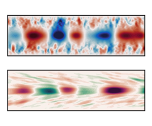In addition to the channel core waves two peaks are revealed near the bounds of the core with wave speeds matching the mean flow velocity, $U$, particularly in the buoyancy spectra. We speculate that these peaks are associated with the hairpin vortices that are ejected into the core from the outer region of the flow (Lloyd et al. Reference Lloyd, Dorrell and Caulfield2022). In penetrating the strongly stratified core they generate large-scale waves whilst being accelerated to the local mean flow velocity before dissipating their kinetic energy.

Figure 5.

The 2-D energy spectra obtained on a spanwise normal slice at $z=L_z/2$. For a given $k_x$, spectra are shown as a function of height $y$ and frequency $\omega$. (a,c) Spectra for $k_x = 2$; (b,d) energy spectra for $k_x = 4$. (a,b) Spectra based on vertical velocity fluctuations; (c,d) spectra based on buoyancy fluctuations. Labels of (c) indicate signals arising from BWs, FWs and hairpin vortex ejection events (HP). Horizontal lines represent bounds of the channel core region: $y=0.8$ and $y=1.2$.

The vertically varying simulation spectra of figure 5 can be compared against vTG solutions by slicing through the dataset at the frequencies associated with the BW and FW, for a given $k_x$, observed in figure 6. The vTG solution growth rates are directly compared against energy spectra at $y=1$ with $k_x=2$ and $k_x=4$. The BWs and FWs are marked with crosses for the vTG solutions and stars for the spectra. The energy contained in the vertically varying structure functions of the identified FW and BW vTG modes, $\hat {v}^{\dagger} \hat {v}$ for vertical velocity and $\hat {b}^{\dagger} \hat {b}$ for buoyancy, are reported in figure 6(b,d,f,h), and compared against $E_{vv}^{2D}(k_x,y,\omega )$ and $E_{bb}^{2D}(k_x,y,\omega )$ at the identified $\omega$ and $k_x$. Direct comparisons are limited by the lack of spanwise structure in the simulation spectra, yet there is reasonable agreement between vTG solutions and simulations when observing their vertical modal structure for the marked modes (figure 6), which peak in the channel core and reduce to zero in the outer regions of the flow. Despite the lack of spanwise structure in the spectra, we see reasonable agreement between linear stability solutions and the spectra for most modes. The BWs are well reproduced aside from buoyancy structure at $(k_x,k_z)=(4,8)$, where we see instability in the outer regions of the flow. This arises due to critical levels, where the local wave speed of the modes matches the background velocity. This behaviour was also reported by Lloyd et al. (Reference Lloyd, Dorrell and Caulfield2022). The majority of the FWs are reasonably well predicted, particularly for the buoyancy structure, although less so than the BWs. We expect that the poorer agreement between vertical velocity spectra and vTG solutions for the FWs is due to the lack of spanwise structure in the spectra, which, as previously discussed, significantly smears the dispersion relation of the FWs. This smearing of the modes could also explain the broader peaks in spectra when compared with vTG solutions, although this could also be due to nonlinear processes at the edge of the core, where interactions with turbulent structures diffuse the sharp peaks.

Figure 6.

Comparison between simulation energy spectra and vTG structure functions for BW and FW (see figure 5). (a,c,e,g) The vTG eigenvalue solutions, growth rate $\sigma$ as a function of temporal frequency $\omega$, for given wavenumbers $k_x$ and $k_z$. Lines represent simulation 2-D energy spectra $E_{vv}^{2D}(k_x,y,\omega )$ at $y=1$ and the same $k_x$ as the vTG solutions. (b,d,f,h) Comparison of the vertical velocity (i) and buoyancy (ii) structure function energies ($\hat {v}^{\dagger} \hat {v}$ and $\hat {b}^{\dagger} \hat {b}$) as a function of height $y$, for the FW and BW modes marked by a cross ($\boldsymbol {\times }$) in (a,c,e,g), respectively. The BW and FW frequencies obtained from the 2-D spanwise-averaged energy spectra of figure 5 for the given $k_x$ are marked as stars ($\star$) in (a,c,e,g). Panels (b,d,f,h) compare their corresponding vertically varying energy spectra $E^{2D}_{vv}$ (i) and $E^{2D}_{bb}$ (ii) at the marked frequency $\omega$ with vTG solutions. In (b,d,f,h), simulation data are marked with solid lines, while vTG solutions are marked with dashed lines.

The linear stability analysis gives a good prediction of channel core dynamics (particularly the dispersion relations of figures 2 and 3), for both the BWs and FWs, once spanwise structure has been taken into account. There are, however, several key open questions regarding the nature of these waves. What are the key processes governing the dispersion and structure of these waves? What are the key parameters and features of the background flow profiles that lead to such a dispersion relation? And what governs the limiting behaviour of the modes, $\omega = U_{max} k_x \pm N_{max}$?

The first of these questions can be answered by assessing the balance between diffusive processes, shear and buoyancy on the vTG solutions. This is achieved by computing the balance of their corresponding terms in the vTG eigenvalue problem (2.15):

(3.1)\begin{equation} \underbrace{-(\lambda + {\rm i} k_x U ) \Delta \hat{v}}_{\mathcal{C}_v} + \underbrace{- \tilde{k}^2 \hat{b}}_{\mathcal{B}_v} + \underbrace{\hat{D}_v \hat{v}}_{\mathcal{D}_v} + \underbrace{{\rm i} k_x \frac{\text{d}^2 U}{\text{d} y^2} \hat{v}}_{\mathcal{S}_v}= 0 \end{equation}

and

(3.2)\begin{equation} \underbrace{-(\lambda + {\rm i} k_x U ) \hat{b}}_{\mathcal{C}_b} + \underbrace{-\frac{\text{d} B}{\text{d} y}\hat{v} }_{\mathcal{B}_b} + \underbrace{\hat{D}_b \hat{b}}_{\mathcal{D}_b}= 0, \end{equation}

where $\mathcal {C}$ represents convective terms, $\mathcal {B}$ represents buoyancy terms, $\mathcal {S}$ represents shear terms, $\mathcal {D}$ represents diffusive terms and the subscripts represent budgets for either the vertical velocity equation ($\hat {v}$) or the buoyancy equation ($\hat {b}$). The balance of these terms at two different values of $\tilde {k}$ and $\tan \theta$ can be observed in figures 7 and 8. The spatial structures of the eigenfunctions for the marked eigenvalues in panels (a) and (b) are reported in panels (c) and (d) for the BW and (e) and (f) for the FW. Here we only report the streamwise and vertical spatial structure of the modes for brevity. The particular values of $\tilde {k}$ and $\tan \theta$ in figures 7 and 8 are chosen as representative of two different regimes. The FW for both small and large $\tilde {k}$ is vertically narrow, particularly for the buoyancy structure, peaking at $y=1$. The vertical structure of the BW appears much wider, and experiences some shearing across the critical levels. When comparing the modal structure of the FW between figures 7 and 8 it is clear that increasing $\tilde {k}$ and $\tan \theta$ leads to a narrower structure. As $\tilde {k}$ grows further and the dispersion relations of both dominant modes tend towards the idealised dispersion relation, their spatial structure narrows and focuses more tightly around the centreline (not shown).

Figure 7.

Modal structure and budgets for the vTG solutions of figure 4 with $\tan \theta = 0$. (a) As per figure 4(a). (b) The growth rate as a function of intrinsic frequency for $\tilde {k} = 4$. The horizontal lines added to (a,b) are as per figure 4. The BWs and FWs are marked with crosses in (a,b), and have their spatial structure and associated budgets reported in (c–j). (c,d,g,h) Associated with BW and (e,f,i,j) associated with FW. (c,e) The vertical velocity spatial structure $v''(x,y) = {\rm Re} (\hat {v}\exp ({\rm i} k_x x))$ and (d,f) the buoyancy spatial structure $b''(x,y) = {\rm Re} (\hat {b}(\exp {\rm i} k_x x))$. (g,i) Vertical velocity budgets in the channel core with labels corresponding to (3.1). (h,j) Buoyancy budgets in the channel core with labels corresponding to (3.2). Line styles in (g–j) represent real components (solid) and imaginary components (dashed). Horizontal dashed lines in (c,d,g,h) represent critical levels where $c = U$.

Figure 8.

Modal structure and budgets for the vTG solutions of figure 4 with $\tan \theta = 4$. The marked modes and corresponding spatial structure and budget plots have $\tilde {k} = 16$. Further details are as per figure 7.

The corresponding budgets of the BW and FW are markedly different from each other for the two choices of $\tilde {k}$ and $\tan \theta$. At low $\tilde {k}$ and $\tan \theta$, the vertical velocity budget for the BW is balanced primarily by the shear and convective terms, with only a small influence of buoyancy and viscosity. In contrast, buoyancy dominates the transport of $\hat {v}$ for the FW, balanced primarily by shear with a weak contribution from convection, at low $\tilde {k}$ and $\tan \theta$. The wavenumber magnitude has a strong influence on this balance. The role of shear is minor for both the FW and the BW at high $\tilde {k}$ and $\tan \theta$, where both modes are governed by the balance between convective and buoyancy terms, with only a small contribution from diffusion and shear. Note that the diffusive term is small at $y=1$ and only influences the solution near the edges of the core where the critical levels are present ($y \approx 0.75$ and $y \approx 1.25$).

The BW therefore transitions from a shear-dominated regime at low $\tilde {k}$ and $\tan \theta$ to a buoyancy-dominated regime at high $\tilde {k}$ and $\tan \theta$. While not shown here, this transition is primarily controlled by $\tilde {k}$, although $\theta$ does play a role by increasing the effective strength of the background stratification, and therefore increasing the buoyancy term of (3.1), as per the Squire transform (Smyth & Carpenter Reference Smyth and Carpenter2019). In contrast to the BW, buoyancy dominates the dynamics of the FW even at low $\tilde {k}$, but shear also influences its dispersion relation until $\tilde {k}$ is large.

It is also informative to assess the influence of the Reynolds and Richardson numbers on the vTG solutions. Noting that the dominant modes are only weakly dependent on the diffusive terms (figures 8 and 9) we approximate the viscous and diffusive coefficients by $A_h = A_v = K_h = K_v = 1/Re_c$. This has a negligible influence on the dispersion relation (further evidence for this is provided in § 3.2, where we investigate solution sensitivity to the background buoyancy and shear profiles), and enables a direct control of the magnitude of the viscous/diffusive terms through $Re_c$. Figure 9 reports the dependence of vTG solutions on $Re_c$ and $Ri_c$ for $k_x = 4$ and $k_z=0$. First note that the Reynolds number only has a weak influence on the solution, only influencing dynamics when $Re_c \lesssim 1000$. It should, however, be appreciated that its influence scales like $\tilde {k}^2$, from inspection of the eigenvalue problem (2.15). We therefore expect the Reynolds number to become more important for large $\tilde {k}$.

Figure 9.

Reynolds (a) and Richardson (b) number dependence of the vTG solutions with background profiles taken from simulation spectra for $k_x = 4$ and $k_z = 0$, as a function of intrinsic frequency $\omega - U_{max} k_x$. The horizontal line represents $\omega = U_{max}k_x = 0$.

In contrast to the Reynolds number, it is clear that the Richardson number has a great influence on the dispersion relation. As $Ri_c$ increases, the intrinsic frequency deviates further from zero for both the BW and FW. Perhaps the most surprising result from figure 9 is that the BW is present, and in fact has its highest (and unstable) growth rate when $Ri_c = 0$. The FW is also present and approximately critically stable, but converges towards $\omega -U_{max} k_x = 0$ as $Ri_c$ reduces. A third mode, between BW and FW, emerges at small Richardson number. This mode (not shown) corresponds to an asymmetric mode with peaks near the edge of the channel core corresponding to the maxima in $U_{yy}$ (figure 1). This mode is also present in other vTG solutions (e.g. figure 4) but is significantly weaker than the dominant modes in the channel.

Of course, the background flow profiles are also sensitive to changes in the Reynolds and Richardson numbers. However, the sensitivity of the modes to $Ri_c$ in isolation of background profiles is highly informative; buoyancy is not a vital component for the BW to emerge, but does have a strong influence on its dispersion. This implies, from inspection of the vTG equations (2.15), that the background shear profile $U_{yy}$ is the vital component for producing these modes. Indeed, assessment of the balance between vTG terms reveals that the BW transitions from a shear-dominated regime to a buoyancy-dominated regime as $\tilde {k}$ increases. Given the BW is primarily governed by shear in the $\tilde {k}$ regime where it dominates, it is perhaps more suitable to refer to these modes as vorticity–gravity waves. While buoyancy is necessary for the suppression of turbulence in the core, and therefore the development of the jet-like velocity profile, shear is the primary control on the development of the dominant backward-propagating vorticity–gravity wave. To further our understanding of the role of buoyancy and shear in the dispersion relation, and vertical structure of the modes, we investigate numerical solutions to the vTG equations using idealised background flow profiles in the following section.

3.2. Linear solutions with idealised base flows

So far we have demonstrated that large-scale waves dominate the core of stratified channel flow, with a strong presence of oblique waves, governed by linear mechanisms. Both forward and backward waves are present, and have a distinct dispersion relation, but it is unclear what properties of the velocity and density profiles lead to such behaviour. This section will develop our understanding of these waves by investigating the numerical solutions to the vTG equations, subject to the flow profiles of figure 10. In addition, we demonstrate that solutions are insensitive to the inclusion of eddy diffusivity. We therefore set $A_H = A_V = K_H = K_V = 1/Re_c$ with $Re_c = 22\,270$, for the idealised flow profiles.

Figure 10.

Velocity and buoyancy profiles with their derivatives, for the idealised stability problems (§ 3.2). (a) Velocity profiles for the $\text {log}$-$\text {sech}$ function (3.3) represented with dash-dotted lines, the $\text {sech}$ function (3.5) represented with dashed lines and the simulation data represented with solid lines. The $\text {log}$-$\text {sech}$ profile is calculated with $w_u^1=12.8$ and the $\text {sech}$ profile with $w_u^2 = 3.6$. (b) First and (c) second derivatives of the velocity profiles in (a). (d) Buoyancy profiles for the $\tanh$ function (3.4) represented with dotted lines and the simulation data represented with solid lines. Idealised profiles are calculated with $Ri_c = 0.293$ and $w_b = 3.9$. (e) The first derivative of the buoyancy profiles in (d). (f) Gradient Richardson number profiles for the simulation data and the continuous idealised profiles.

All idealised profiles are based upon the characteristics of those obtained through the nonlinear simulations, with a velocity maximum at $y=1$ and no-slip boundaries at $y=0$ and $y=2$, normalised by the channel half-height. Here, the velocity scale is taken as the velocity maximum, $u_c$, such that $Ri_c = \Delta \rho g \delta / \rho _0 u_c^2$. Assuming the velocity maximum and corresponding negative $U_{yy}$ are the key drivers governing the dispersion of these waves, we first obtain solutions for a $\text {log}$-$\text {sech}$ velocity profile and a $\tanh$ buoyancy profile:

(3.3)\begin{equation} U = \frac{1}{ \ln (\cosh(w_u^1))}\ln \left(\frac{\text{sech}(w_u^1(y-1))}{{\rm sech}(w_u^1)}\right) \end{equation}

and

(3.4)\begin{equation} B = Ri_c \tfrac{1}{2}\tanh(w_b(y-1)). \end{equation}

Here $w_u^1$ and $w_b$ control the ‘sharpness’ of the velocity and buoyancy interfaces at $y=1$. This particular choice of buoyancy profile is well motivated due to the close agreement with simulation data, aside from near-wall statistics far from the channel core. The velocity profile is chosen assuming that the key feature required to reproduce the dominant modes is the large negative peak in $U_{yy}$ at the centreline, and other complexities can be neglected. Like the nonlinear simulation profiles, at $y=1$ these idealised profiles have a velocity maximum, a minimum in $U_{yy}$ and a maximum in $B_y$. Parameter values are chosen such that $U_{yy}$ and $B_y$ coincide with simulation data at $y=1$ (figure 10): $w_u^1 = 12.8$, $w_b = 3.9$ and $Ri_c = 0.293$.

In addition to the $\text {log}$-$\text {sech}$ velocity profile, solutions are also sought for $\text {sech}$ profiles of the form

(3.5)\begin{equation} U = \frac{\text{sech}(w_u^2(y-1)) -\text{sech}(w_u^2)}{1-\text{sech}(w_u^2)}. \end{equation}

This choice leads to both a minimum in $U_{yy}$ at $y=1$ and two maxima either side of the core region. With $w_u^2 = 3.6$ the minimum in $U_{yy}$ matches that of the simulation data. The magnitudes of the two maxima in $U_{yy}$ are approximately consistent with simulation data (figure 10), although their location is further from the centreline than simulation profiles. Regardless, this choice of profile enables assessment of the role of these maxima on the dominant modes.

Figure 10(f) shows the gradient Richardson number, $Ri_g = N^2 / S^2$ with $S = U_y$, for the simulation solutions and the analytical profiles, as a measure of stability. All three sets of profiles obtain a buoyancy-dominated core region (high $Ri_g$) and a shear-dominated outer region (low $Ri_g$). The two sets of idealised profiles show lower $Ri_g$ in the outer regions than the simulation profiles, but do obtain a similar $y$ value where $Ri_g \approx 0.2$, before rapidly increasing in the channel core.

Solutions to the vTG equations are sought for both sets of profiles, following the numerical procedure outlined in § 2.2.

The dispersion relation obtained using the $\text {log}$-$\text {sech}$ velocity profile and $\tanh$ buoyancy profile is shown in figure 11, and directly compared with the dominant modes of § 3.1. There are clear similarities between these solutions and the nonlinear simulations. The simplified system obtains the same two dominant modes and correctly predicts their limiting behaviour at large $\tilde {k}$. The FW is predicted in excellent agreement with the reference profiles. There are two notable differences between figures 11 and 4. Firstly, while there is a turning point in the dispersion relation for the BW in both the idealised vTG solutions and those based on simulation profiles, the idealised system reaches the turning point at a lower $\tilde {k}$ than the simulation-based solutions. Secondly, the reduced system has a third dominant mode at a very low and negative intrinsic frequency. This mode corresponds to instabilities at the boundaries rather than the core of the channel and is therefore ignored in this study.

Figure 11.

Dispersion relation predictions for vTG solutions, visualised using the growth rate $\sigma$, for the idealised $\text {log}$-$\text {sech}$ velocity profile (3.3) and $\tanh$ buoyancy profile (3.4). Solutions obtained with increasing angles of obliquity: (a) $\tan \theta = 0$, (b) $\tan \theta = 1$, (c) $\tan \theta = 2$ and (d) $\tan \theta = 4$. Dashed lines represent reference leading-order modes (BW and FW) obtained for the system using nonlinear simulation profiles (figure 4). Horizontal lines represent idealised dispersion relations based on $U_{max}$ and $N_{max}$, as detailed in figure 1(c).

The dispersion relations obtained using the $\text {sech}$ velocity profile are shown in figure 12. Solutions are similar to those of the $\text {log}$-$\text {sech}$ profiles and the simulation data; at high $\tilde {k}$ both dominant modes collapse to the same limiting behaviour, and the FW is reproduced over the full $\tilde {k}$ and $\theta$ range. The only region where differences emerge is for the BW at low $\theta$ and low $\tilde {k}$, where the $\text {sech}$ profile leads to a larger deviation from the reference dispersion relation. Given the buoyancy profile is reasonably consistent between both idealised profiles and the reference profile (figure 10), the deviation of BW solutions from the reference data at low $\theta$ and $\tilde {k}$ is consistent with previous findings, since this is the region where shear is the dominant mechanism generating the BW.

Figure 12.

Dispersion relation predictions for vTG solutions, visualised using the growth rate $\sigma$, for the idealised $\text {sech}$ velocity profile (3.5) and $\tanh$ buoyancy profile (3.4). Solutions obtained with increasing angles of obliquity: (a) $\tan \theta = 0$, (b) $\tan \theta = 1$, (c) $\tan \theta = 2$ and (d) $\tan \theta = 4$. Dashed lines represent reference leading-order modes (BW and FW) obtained for the system using nonlinear simulation profiles (figure 4). Horizontal lines represent idealised dispersion relations based on $U_{max}$ and $N_{max}$, as detailed in figure 1(c).

Solutions obtained for the two idealised profiles and profiles of the nonlinear simulations are directly compared in figure 13, for $\theta = 0$. Dispersion relations for the dominant modes are directly compared in figure 13(a), and the vertically varying structure functions for the BW and FW at $\tilde {k} = 4$ are compared in figure 13(b–e). In addition to the data obtained using vertically varying eddy viscosity/diffusivity coefficients (detailed in § 2.2) solutions are also shown for constant coefficients ($\nu = \kappa = 1/Re_c$) respectively denoted turb. and lam. in figure 13. Dispersion relations for the two sets of solutions are indistinguishable, as are their structure functions, aside from the buoyancy functions for the BW in the region of the critical levels, where the increased viscosity associated with the turb. solutions smooths the local peak. This further justifies the choice of constant viscosity/diffusivity for the idealised solutions. Of particular note is the close agreement between the structure functions of all four sets of solutions, aside from the buoyancy structure for the BW at the region of the critical levels. Differences in the shear profiles leads to only minor differences in the vertical structure of the dominant modes. Qualitatively, the dominant modes observed in the channel core of nonlinear simulations can be reproduced with a simple idealised velocity and buoyancy profile consisting of a velocity maximum, a negative $U_{yy}$ and maximum in $B_y$, at the centreline.

Figure 13.

Comparisons between vTG solutions obtained using nonlinear simulation profiles and idealised profiles for $\theta = 0$. Reference profiles are obtained with a constant viscosity/diffusivity (lam.) and a turbulent viscosity/diffusivity (turb.). Idealised profiles are the $\text {log}$-$\text {sech}$ and $\text {sech}$ velocity profiles with the $\tanh$ buoyancy profile. (a) The dispersion relations for the dominant modes and (b–e) vertically varying structure functions at $\tilde {k} = 4$, marked by the vertical dashed line in (a).

The limiting behaviours of the dispersion relations for both the FW and BW have been consistent for all vTG solutions so far, tending towards $\omega - U_{max} k_x = \pm N_{max}$ as $\tilde {k} \rightarrow \infty$. Given that buoyancy dominates the flow over buoyancy at large $\tilde {k}$ (figures 7 and 8) four further vTG solutions are sought for shear-free velocity profiles ($U=1$) and $\tanh$ buoyancy profiles (3.4), with varying values of $Ri_c$ and $w_b$, hypothesising that the thickness of the buoyancy interface, and the buoyancy gradient at the centreline, are the key controls on this limiting behaviour. The dispersion relations for these additional cases can be observed in figure 14.

Figure 14.

Dispersion relation predictions for vTG solutions, visualised using the growth rate $\sigma$, based upon a shear-free ($U=1$) flow with a $\tanh$ buoyancy profile (3.4). All solutions are obtained with $\tan \theta = 0$. (a–d) Solutions obtained with different values of $w_b$ and $Ri_c$, but with consistent buoyancy gradients at the centreline, $\max (B_y) = \tfrac {1}{2} Ri_c w_b$. Lines represent idealised dispersion relations based on $U_{max}$ and $N_{max}$, detailed in figure 4.

The four values of $Ri_c$ and $w_b$ have been chosen such that $N_{max} = \max (B_y) = \frac {1}{2} w_b Ri_c$ is consistent for all cases, and with the nonlinear simulation data. The dispersion relations obtained for the flows free from shear are symmetric about $\omega - U_{max} k_x = 0$; the BW and FW modes are equal but opposite in sign. This is an unsurprising result, but confirms that the asymmetry between the FW and BW of the non-uniform velocity profiles arises due to the influence of shear (this is revisited in § 3.3). The FW and BW dispersion relations of the shear-free flows tend towards the same solutions as those with shear of figures 11 and 12 at high $\tilde {k}$. The key difference between the four cases of figure 14 is the rate at which the FWs and BWs converge towards the limiting behaviour, $\omega - U_{max} k_x = \pm N_{max}$ as $\tilde {k}$ increases. A small value of $w_b$ leads to quicker convergence towards the high-$\tilde {k}$ limit than when $w_b$ is larger. In other words, the sharper the density interface (higher $w_b$), the slower the convergence towards the idealised dispersion relation.

The limiting behaviour of the shear-free system can be explained by this behaviour, noting that as $\tilde {k}$ increases, the vertical extent of the dominant modes reduces and focuses more tightly around the channel centreline (see figures 7 and 8, and related discussion). As this occurs, the buoyancy gradient across the vertical extent of the dominant modes tends towards an approximately constant value, depending on the interface thickness (controlled by $w_b$). Therefore, as $\tilde {k}$ increases, the dominant modes tend towards the idealised dispersion relation for a system with a constant buoyancy gradient. A thinner buoyancy interface (higher $w_b$) requires narrower spatial modes before this limit is reached, shifting convergence towards the limiting behaviour towards higher $\tilde {k}$. This can be readily extended to the sheared profiles of the nonlinear simulations and the idealised systems, given that the influence of shear reduces as $\tilde {k}$ increases, until eventually buoyancy dominates the flow. Therefore, as $\tilde {k}$ is increased, the system behaves as if shear were negligible and the buoyancy frequency was constant, leading to the limit $\omega = U_{max} k_x \pm N_{max}$.

To summarise this section, it has been demonstrated that the crucial ingredients required to qualitatively reproduce the dominant modes observed in the core of turbulent stratified plane Poiseuille flow are a velocity maximum, with a corresponding negative $U_{yy}$, intersecting a region of strong buoyancy gradient. The limiting behaviour of the dominant mode dispersion relations, $\omega - U_{max} k_x = \pm N_{max}$, at high $\tilde {k}$ arises due to the negligible influence of shear at high wavenumbers, and the reduced vertical extent of the dominant modes, such that the local flow tends towards that of a shear-free flow with a constant buoyancy gradient. Changes in the shear profile affect the backward-propagating mode at low wavenumbers, but have little influence on the forward-propagating mode. A potential explanation for this asymmetry is provided in the following section, where we explore analytical solutions to the inviscid TG equations using piecewise profiles.

3.3. Analytical inviscid solutions

An open question remains regarding the differences between the FW and BW at low $\tilde {k}$, where the BW is governed primarily by shear with a weak dependence on buoyancy and the FW is governed by buoyancy with a weaker dependence on shear. Here we explore analogous solutions to the inviscid TG equations using piecewise velocity and buoyancy profiles as an approximation to the smooth profiles of § 3.2 (figure 10). Inviscid analytical solutions to the piecewise TG equations have been invaluable for the study of instabilities in stratified shear flows (Baines & Mitsudera Reference Baines and Mitsudera1994; Caulfield Reference Caulfield1994; Carpenter et al. Reference Carpenter, Tedford, Heifetz and Lawrence2011; Smyth & Carpenter Reference Smyth and Carpenter2019), and are particularly insightful due to their interpretability. It is of course anticipated that resultant dispersion relations will comprise interfacial waves, with dispersion relations largely inconsistent with those obtained for the smooth profiles of §§ 3.1 and 3.2. Yet despite this, this section shows that there are key similarities between the solutions, offering a potential explanation to the disparity between the influence of shear on the BW and FW.

The inviscid TG equations are obtained from the vTG eigenvalue problem (2.15). Neglecting the terms $\hat {D}_v \hat {v}$ and $\hat {D}_b \hat {b}$, and relating the eigenvalues $\lambda$ to the wave speed $c$ by $\lambda = -{\rm i} k_x c$ leads to the differential eigenvalue problem (Smyth & Carpenter Reference Smyth and Carpenter2019)

(3.6)\begin{equation} \hat{v}_{yy} + \left[ \frac{\tilde{k}^2}{k_x^2} \frac{B_y}{ (U - c)^2 } - \frac{ U_{yy}}{ (U - c)} - \tilde{k}^2 \right] \hat{v} = 0. \end{equation}

Note that the wave-vector angle appears only through the buoyancy term, $\tilde {k}^2 / k_x^2 = 1 / \cos ^2 \theta$. We seek solutions to piecewise velocity and buoyancy profiles:

(3.7)\begin{equation} U = \begin{cases} 2 - y, & y \geq 1, \\ y, & y \leq 1, \end{cases} \end{equation}

where $U_{max} = 1$, and

(3.8)\begin{equation} B = Ri_c\begin{cases} 0.5, & y \geq 1, \\ -0.5, & y \leq 1. \end{cases} \end{equation}

These profiles are discontinuous in $U_{y}$ and $B$, such that $U_{yy} = -2 \delta (y-1)$ and $B_y = Ri_c \delta (y-1)$, where $\delta ()$ is the Dirac delta function and $Ri_c = 0.293$, consistent with vTG solutions of §§ 3.1 and 3.2. These profiles are a piecewise approximation to the log-sech velocity and tanh buoyancy profiles of figure 10, with a velocity maximum and a buoyancy interface at the channel centreline. We seek solutions to the TG equations subject to the piecewise profiles with Dirichlet boundary conditions $\hat {v} = 0$ at $y=0$ and $y=2$.

The general solution to (3.6) for the piecewise velocity (3.7) and buoyancy (3.8) profiles is

(3.9)\begin{equation} \hat{v} = \begin{cases} A \,{\rm e}^{-\tilde{k}(y-1)} - A\, {\rm e}^{\tilde{k}(y-3)} \quad y \geq 1, \\ A \,{\rm e}^{\tilde{k}(y-1)} - A \,{\rm e}^{-\tilde{k}(y+1)} \quad y \leq 1, \end{cases} \end{equation}

where $A$ is a constant. The dispersion relation is obtained by substitution of $\hat {v}$ into the TG equations (3.6) and integrating over the interface at $y=1$, with $U_{yy} = -2 \delta (y-1)$ and $B_y = Ri_c \delta (y-1)$, derived from (3.7) and (3.8), leading to

(3.10)\begin{equation} (c-1)^2 + c_v (c-1) - c_g^2 = 0 , \end{equation}

assuming $Ri_c \neq 0$. The wave speeds $c_v = F/ \tilde {k}$ and $c_g^2 = F Ri_c / 2 \tilde {k} \cos ^2 \theta$ represent the solutions obtained if the system were solved for either $Ri_c = 0$ or $U = 1$, respectively, resulting in a backward-propagating isolated vorticity wave with $c - 1 = -c_v$, or two interfacial gravity waves with $c-1 = \pm c_g$. Note that only a single vorticity wave is produced when $Ri_c = 0$, travelling backwards relative to the background flow. The factor $F = (1-{\rm e}^{-2 \tilde {k}})/(1+{\rm e}^{-2 \tilde {k}})$ arises due to the imposed boundary conditions, and is bounded between 0 and 1 for $k \in [0,\infty )$, respectively. If the system were instead solved for boundary conditions where $\hat {v} \rightarrow 0$ at $y \rightarrow \pm \infty$, the dispersion relation would satisfy (3.11) with $F=1$; thus the Dirichlet boundary conditions only affect the solution for small $\tilde {k}$. This is reasonable given that small instabilities (large $\tilde {k}$) are more isolated from the boundaries than larger instabilities (small $\tilde {k}$).

Subsequently, the dispersion relation can be obtained, assuming $Ri_c > 0$:

(3.11)\begin{equation} c - 1 = c - U_{max} =- c_v \pm \sqrt{ c_g^2 + c_v^2}. \end{equation}

The wave speed $c$ is purely real (assuming $Ri_c > 0$), such that the system is marginally stable with $\omega = k_x \,{\rm Re}(c) = k_x c$ and $\sigma = 0$.

The dispersion relation $\omega (k_x)$ of the piecewise system is visualised in figure 15. Here we report the intrinsic frequency at $y=1$, $\omega - U_{max} k_x$, as a function of wavenumber magnitude $\tilde {k}$, for varying angles of obliquity $\theta$ and Richardson numbers $Ri_c$. These are compared against the frequencies obtained for isolated vorticity and interfacial gravity waves $\omega - U_{max} k_x = - \omega _v$ and $\omega - U_{max} k_x = \pm \omega _g$, respectively, where $\omega _v = c_v k_x = F \cos \theta$ and $\omega _g^2 = c_g^2 k_x^2 = F \tilde {k} Ri_c / 2$. By construction, two modes are present for a given $\tilde {k}$: a forward-propagating mode with positive intrinsic frequency and a backward-propagating mode with negative intrinsic frequency. At high $\tilde {k}$ both modes tend towards the dispersion relation for interfacial gravity waves, $\pm \omega _g$. At low $\tilde {k}$ the BW dispersion relation tends towards $-\omega _v$, most clear in figure 15(a) at $\tan \theta = 0$. The transition of the BW between $\omega - U_{max} k_x \approx -\omega _v$ at low $\tilde {k}$ and $\omega - U_{max} k_x \approx -\omega _g$ at high $\tilde {k}$ represents a transition between shear-controlled and buoyancy-controlled flow, which is dependent on $\theta$ and $Ri_c$; increasing these parameters increases the rate of transition towards buoyancy-dominant flow, both through an increase of $c_g^2$ relative to $c_v^2$ in the dispersion relation (3.11). The influence of shear on the FW is not so clear but is certainly less than on the BW (see figure 15a with $\tan \theta = 0$); at low $\tilde {k}$, the discrepancy between the dispersion relation and that of an interfacial gravity wave is larger for the BW than the FW. This asymmetry can be explained by the lack of a FW when the flow is free from a buoyancy interface, where only a backward-propagating isolated vorticity wave is present. In addition, from inspection of the dispersion relation (3.11), one notes that the two contributions of shear ($c_v$) have opposite signs when the positive FW root is taken, thus partially cancelling out, unlike the negative BW root. This is complicated by the nonlinearity of the dispersion relation, but is supported by the limiting behaviour observed in figure 15(a). Asymmetry between the BW and FW therefore arises due to the imbalance between shear contributions towards the FW and the BW.

Figure 15.

Dispersion relation obtained for the piecewise velocity and buoyancy profiles (3.11) visualised using the intrinsic frequency $\omega - U_{max} k_x$ as a function of the wavenumber magnitude $\tilde {k}$ (solid lines). (a) Dispersion relation for $Ri_c = 0.293$ over a range of $\tan \theta$; (b) dispersion relation for $Ri_c = 1$ over a range of $\tan \theta$; (c) dispersion relation for $\theta = 0$ over a range of $Ri_c$. Dashed lines represent the dispersion relation for isolated vorticity waves, $\omega - U_{max} k_x = - c_v k_x$, and dash-dotted lines represent the dispersion relation for interfacial gravity waves, $\omega - U_{max} k_x = \pm c_g k_x$.

There are clear similarities between the dispersion relation for the piecewise system and that of the smooth vTG solutions, particularly the log-sech velocity profile and tanh buoyancy profile (figure 11). Both systems lead to two dominant modes with $\sigma \leq 0$: a forward-propagating wave and a backward-propagating wave, relative to the velocity at the centre of the channel. Buoyancy dominates the dispersion relation of these two modes at high $\tilde {k}$, while shear becomes important for small $\tilde {k}$. The transition between these two regimes is controlled by $Ri_c$ and $\theta$. In addition, both systems lead to a clear asymmetry between the two modes at low $\tilde {k}$ due to the influence of shear, which dominates the dispersion relation for the BW at low $\tilde {k}$. For $Ri_c = 0.293$ and $\theta = 0$ there is evidence that the BW transitions away from the shear-dominant regime for $\tilde {k} \approx O(1)$ (see figures 11 and 15).

However, there is a clear disagreement between the two systems regarding the limiting behaviour of the dispersion relations: the dispersion relation for the piecewise system tends towards that of interfacial gravity waves while the smooth system tends to that of idealised gravity waves in a region of zero shear and constant buoyancy frequency. Nevertheless, the similarities between the two systems regarding the role of shear and buoyancy provides a potential explanation to the importance of shear for the BW and the asymmetry that develops between the two leading-order modes. The piecewise system shows that the BW emerges as a vorticity wave at low $\tilde {k}$ with only a minor influence from buoyancy, while the FW is dependent on buoyancy to propagate.

However, the linear framework so far has been unable to establish why the BWs dominate spectra in the nonlinear simulations, with energy several orders of magnitude larger than their forward-propagating counterpart. In the following section we revisit the stochastic models developed by Lloyd et al. (Reference Lloyd, Dorrell and Caulfield2022) and demonstrate that it is the nature of the forcing to the linear system that leads to the disparity in energy content between the two waves.

3.4. Stochastically forced simulations

So far, we have demonstrated that both the BW and FW of the nonlinear system are well predicted by linear stability analysis in all but their respective energy content. Here we revisit the stochastically forced 2-D linear framework of Lloyd et al. (Reference Lloyd, Dorrell and Caulfield2022) to investigate the influence of the forcing structure on channel core dynamics. This framework is developed from the perturbation equations (2.7) and (2.8) but approximates inner- and outer-region turbulence using white-noise forcing. With this model, Lloyd et al. (Reference Lloyd, Dorrell and Caulfield2022) were able to predict the BW in excellent agreement with nonlinear simulations, but were unable to explain the weaker mode with positive intrinsic frequency which was seemingly in disagreement with simulation spectra. Now recognising that differences arose due to the neglect of spanwise structure in the interpretation of simulation spectra, it is worth revisiting this body of work since, despite the model neglecting nonlinear terms, it was able to predict the dominance of the BW compared with the weaker mode, which we now recognise as the FW with $k_z=0$. Despite the two dominant modes arising with similar growth rates in the vTG solutions (or, indeed, with growth rates favouring the FW), the stochastic model of Lloyd et al. (Reference Lloyd, Dorrell and Caulfield2022) was able to predict the dominance of the BW observed in nonlinear simulations. We therefore hypothesise that the dominance of the BW must arise through the forcing conditions of stratified channel flow, but is ultimately still governed by linear processes. In particular, the inner-/outer-layer turbulence perturbs the channel core with ejections of low-momentum fluid into the channel core; such low-momentum fluid preferentially generates BWs, due to its low velocity compared with the faster jet-like core.

To test this hypothesis we repeat the simulations of Lloyd et al. (Reference Lloyd, Dorrell and Caulfield2022) but with forcing applied directly to the channel core, with no external inner/outer forcing. In this way, BW and FW should be generated with approximately equal energy content. For clarity we briefly describe the model here, and refer the reader to Lloyd et al. (Reference Lloyd, Dorrell and Caulfield2022) for further details. We introduce the streamfunction $\psi ^+$, where $(u'')^+ = \partial \psi ^+ / \partial y$ and $(v'')^+ = - \partial \psi ^+ / \partial x$. The superscript $+$ represents variables scaled by the friction velocity $u_\tau$, noting this is a more appropriate scale for the inner- and outer-region turbulence. The difference in spectral energy content between the FW and BW is largest for purely streamwise-propagating flow ($k_z=0$); thus we restrict our stochastic formulation to two dimensions. While we have shown that three-dimensionality is critical for a clear interpretation of the dominant modes in the nonlinear simulations, the aim of the section is to test the hypothesis that the spatial location of the stochastic forcing is a key control on the energy content of the two resultant modes, which, as we show, can be convincingly demonstrated using the 2-D model. Rescaling and substituting $\psi ^+$ into the perturbation equations (2.7) and (2.8) leads to

(3.12)\begin{equation} \frac{\partial{}}{\partial{t^+}}\nabla^2 \psi^++ U^+ \frac{\partial{}}{\partial{x}}\nabla^2 \psi^+- \frac{\text{d}^2 U^+}{\text{d} y^2}\frac{\partial{\psi^+}}{\partial{x}} =- \frac{\partial{b^+}}{\partial{x}} + \frac{1}{Re_\tau} \nabla^4 \psi^++ \mathcal{W}(y) \end{equation}

and

(3.13)\begin{equation} \frac{\partial{(b'')^+}}{\partial{t^+}} + U^+ \frac{\partial{(b'')^+}}{\partial{x}} - \frac{\text{d} B^+}{\text{d} y}\frac{\partial{\psi^+}}{\partial{x}} = \frac{1}{Pr \,Re_\tau} \nabla^2 (b'')^+. \end{equation}

Here the buoyancy fluctuations are given by $(b'')^+ = -Ri_\tau \rho '$ and $\mathcal {W}(y)$ represents vertically correlated stochastic forcing to the linear system, approximating nonlinear processes. These simulations use the background flow parameters and profiles of the nonlinear simulations (figure 1), and specify

(3.14)\begin{equation} \mathcal{W}(y) = \xi(y) \mathcal{N}(0,1/ \Delta t ), \end{equation}

where $\mathcal {N}$ represents a normal distribution with a variance scaled by the simulation time step $\Delta t$. The function $\xi (y)$ defines the vertical structure of $\mathcal {W}(y)$. We investigate solutions using two smooth structure functions which respectively force either the inner/outer regions of the flow or the channel core. Following Lloyd et al. (Reference Lloyd, Dorrell and Caulfield2022), the first function, termed ‘outer forced’, is given by $\xi _o(y) = \nu _t / \max (\nu _t)$, where $\nu _t = - \overline {u'v'}/\bar {u}_y$. The second function, termed ‘core forced’, is taken as

(3.15)\begin{equation} \xi_c(y) = \tfrac{1}{2} \tanh(100(y-0.98)) - \tfrac{1}{2} \tanh(100(y-1.02)), \end{equation}

such that forcing is applied only to a narrow region in the core of the channel. Subscripts $o$ and $c$ refer to either ‘outer’ or ‘core’ forcing. The ‘outer’ forcing is designed to approximate the perturbations felt in the nonlinear simulations due to outer-region turbulence, while the ‘core’ forcing is a hypothetical alternative where perturbations are generated at the region of maximum velocity, or the centre of the BW and FW eigenfunctions.

The system of equations is discretised and solved using Dedalus (Burns et al. Reference Burns, Vasil, Oishi, Lecoanet and Brown2020). Equations are solved on a 2-D domain of size $L_x \times L_y = 8 {\rm \pi}\times 2$, discretised using a Fourier basis in the periodic ($x$) direction and a Chebyshev basis in the vertical ($y$) direction, dealiased using the $3/2$ rule. The grid resolution is set to $N_x \times N_y = 512 \times 256$ approximately equal to the grid resolution of the nonlinear simulations (§ 2.1). At each time step the stochastic forcing is generated on a grid half this size: $\mathcal {W}(y)$ is calculated from the normal distribution $\mathcal {N}$ at each grid point of the coarse grid before up-sampling to the correct resolution. The initial-value problem, initially at rest, is integrated in time using a first-order Runge–Kutta scheme for a total simulation time of $T^+=100$, where the flow reaches a pseudo-steady state at $T^+ \approx 20$.

Snapshots of instantaneous data from the stochastically forced simulations are presented in figure 16. Under ‘outer’ forcing conditions, there is a clear dominant streamwise wavenumber in the core of the channel, corresponding to the BW. In contrast, ‘core’ forcing leads to a clear presence of multiple streamwise wavenumbers with different vertical extent. The lower magnitude of modes in the ‘core’ forced simulations can be explained by the lower energy input of $\mathcal {W}(y)$, which acts only in a narrow region in the channel core. Despite this, there is a clear signal from multiple modes for the ‘core’ forced simulation.

Figure 16.

Snapshots of instantaneous data from the stochastically forced simulations. (a,c,e) ‘Outer’ forced simulations. (b,d,f) ‘Core’ forced data. (a,b) Vertical velocity perturbations, (c,d) buoyancy perturbations and (e,f) white noise forcing functions, scaled by the simulation time step.

The 2-D energy spectra for the buoyancy fluctuations are presented in figure 17 showing clear agreement with vTG solutions and nonlinear simulation spectra (figures 2a and 3a). Consistent with nonlinear simulations (figure 3) and the stochastic model of Lloyd et al. (Reference Lloyd, Dorrell and Caulfield2022), ‘outer’ forcing leads to a dominant BW with an energy several orders of magnitude higher than that of the FW. By forcing the system directly at the channel core, we find that both the BW and the FW are strongly present in the spectra. Further, while both modes are clearly present and near equal in order of magnitude, the FW has a higher energy content than the BW, in agreement with the vTG solutions which show a marginally lower growth rate for the BW across most $\tilde {k}$ (figure 4).

Figure 17.

Dispersion relation for the stochastically forced linear simulations, visualised with the 2-D buoyancy perturbation energy spectra $E_{bb}^{2D}$. (a) ‘Outer’ forced simulation data. (b) ‘Core’ forced simulation data. Lines are as per figure 2(a), with dash-dotted lines representing vTG solutions of § 3.1.

These simulations therefore demonstrate that the dominance of the BWs in the core of stratified channel flow can potentially be explained by the low momentum of outer-region activity, relative to the high momentum of the channel core. If instead perturbations were centred at the region of highest velocity, both sets of waves would be approximately equal in energy content.