2.1. State space $\mathbb{N}_0$

Let $\{X_t \,:\, t\geq0\}$ be a birth–death process on $\mathbb{N}_0$ with infinitesimal operator $\mathcal{A}$ given by the semi-infinite tridiagonal matrix

(1) \begin{equation}\mathcal{A}=\begin{pmatrix}-(\lambda_0+\mu_0)& \quad \lambda_0&&&&\\[3pt]\mu_1& \quad -(\lambda_1+\mu_1)& \quad \lambda_1&&&\\[3pt]&\quad \mu_2& \quad -(\lambda_2+\mu_2)& \quad \lambda_2&&\\[3pt]&&\quad \ddots& \quad \ddots& \quad \ddots\end{pmatrix}.\end{equation}

A diagram of the transitions between states is

We will assume that the set of rates $\{\lambda_n, \mu_n\}$ uniquely determines the birth–death process. Define the potential coefficients $(\pi_n)_{n\in\mathbb{N}_0}$ as

\begin{equation*}\pi_0=1,\quad\pi_n=\frac{\lambda_0\lambda_1\cdots \lambda_{n-1}}{\mu_1\mu_2\cdots \mu_n},\quad n\in\mathbb{N}.\end{equation*}

These coefficients are defined as the solutions of the symmetry equations $\mathcal{A}_{ij}\pi_i=\mathcal{A}_{ji}\pi_j$ , $i,j\in\mathbb{N}_0,$ normalized by the condition $\pi_0=1$ (see [Reference Karlin and McGregor20, p. 494]). Since $\mathcal{A}$ is tridiagonal, these symmetry equations are equivalent to $\pi_n\mu_n=\lambda_{n-1}\pi_{n-1}$ for $n\geq1$ . If we assume that $\mathcal{A}$ is a closed, symmetric, self-adjoint, and negative operator in the Hilbert space $\ell^2_{\pi}(\mathbb{N}_0)$ , then, applying the spectral theorem (see [Reference Karlin and McGregor20]), we can obtain an integral representation of the transition probability functions $P_{ij}(t)=\mathbb{P}\!\left(X_t=j\,|\, X_0=i\right)$ in terms of a nonnegative measure $\psi(x)$ supported on $[0,\infty)$ and a family of polynomials $(Q_n)_{n\in\mathbb{N}_0}$ , generated by the three-term recurrence relation with initial conditions

(2) \begin{equation}\begin{split}Q_0(x)&=1,\quad Q_{-1}(x)=0,\\-xQ_n(x)&=\lambda_nQ_{n+1}(x)-(\lambda_n+\mu_n)Q_n(x)+\mu_nQ_{n-1}(x),\quad n\in\mathbb{N}_0.\end{split}\end{equation}

Observe that if we define $Q(x)=(Q_0(x),Q_1(x),\ldots)^T$ , then Q(x) is just the eigenvector in the eigenvalue equation $-xQ(x)=\mathcal{A}Q(x)$ . This integral representation, called the Karlin–McGregor formula (see [Reference Karlin and McGregor20]), is given by

(3) \begin{equation}P_{ij}(t)=\pi_j\int_{0}^{\infty}e^{-xt}Q_i(x)Q_j(x)d\psi(x),\quad i,j\in\mathbb{N}_0.\end{equation}

In [Reference Karlin and McGregor19], several probabilistic properties of the birth–death processes were studied in terms of the spectral measure. For instance, the birth–death process is recurrent if and only if $\int_0^\infty x^{-1}d\psi(x)=\infty$ $\big($ also equivalent to $\sum_{n=0}^\infty (\lambda_n\pi_n)^{-1}=\infty\big)$ . Otherwise it is transient. If the process is recurrent, then it is positive recurrent if and only if the spectral measure $\psi$ has a finite jump at $x = 0$ of size $\psi(\{0\})=\left(\sum_{n=0}^\infty\pi_n\right)^{-1}$ . Otherwise it is null recurrent. Other quantities, such as the moments of the first passage time distributions, quasi-stationary distributions, or limit theorems, can also be studied using the Karlin–McGregor representation. The reader is invited to consult [Reference Domínguez de la Iglesia9, Reference Van Doorn35, Reference Schoutens30, Reference Schrijner31] for a collection of some of these results.

An important role for the birth–death process is played by the function

(4) \begin{equation}\Omega_{j,n}(t)=\lambda_{n-1}P_{j,n-1}(t)-\mu_nP_{j,n}(t),\quad j,n\in\mathbb{N}_0,\quad\lambda_{-1}=0,\end{equation}

describing the probability current in the state n at time t, given that we start at state j (see [Reference Gillespie12, p. 383]). The function $\Omega_{j,n}(t)$ represents a net probability flux from state $n-1$ to state n at time t. The importance of this function is that it is related to the Kolmogorov forward equations for birth–death processes, given by

(5) \begin{equation}\begin{split}\frac{\partial}{\partial t}P_{j,0}(t)&=-(\lambda_0+\mu_0)P_{j,0}(t)+\mu_1P_{j,1}(t)=\Omega_{j,0}(t)-\Omega_{j,1}(t),\\[3pt]\frac{\partial}{\partial t}P_{j,n}(t)&=\lambda_{n-1}P_{j,n-1}(t)-(\lambda_n+\mu_n)P_{j,n}(t)+\mu_{n+1}P_{j,n+1}(t)=\Omega_{j,n}(t)-\Omega_{j,n+1}(t).\end{split}\end{equation}

This function gives a discrete version for a similar situation applied to the Kolmogorov forward equation (or Fokker–Planck equation) for diffusion processes (see [Reference Gillespie12, p. 121]), replacing the partial derivative by an integer-valued analogue. The function $\Omega_{j,n}(t)$ has been recently considered in [Reference Giorno and Nobile13, Reference Giorno and Nobile14] to obtain functional relations between the transition probabilities of a birth–death process on $\mathbb{N}_0$ and the transition probabilities of a bilateral birth–death process (see for instance [Reference Giorno and Nobile13, Proposition 5]). Using the Karlin–McGregor formula (3) and the symmetry property $\pi_n\mu_n=\lambda_{n-1}\pi_{n-1}$ , we can write $\Omega_{j,n}(t)$ as

\begin{equation*}\Omega_{j,n}(t)=\mu_n\pi_n\int_0^{\infty}e^{-xt}Q_j(x)\left[Q_{n-1}(x)-Q_n(x)\right]d\psi(x),\quad j,n\in\mathbb{N}_0.\end{equation*}

If we define the dual polynomials $(H_n)_{n\in\mathbb{N}_0}$ (see [Reference Karlin and McGregor20, Reference Karlin and McGregor19]) by

\begin{equation*}H_0(x)=\mu_0,\quad H_{n+1}(x)=\lambda_n\pi_n\left[Q_{n+1}(x)-Q_n(x)\right],\quad n\in\mathbb{N}_0,\end{equation*}

then we can write $\Omega_{j,n}(t)$ as

\begin{equation*}\Omega_{j,n}(t)=-\int_0^{\infty}e^{-xt}Q_j(x)H_n(x)d\psi(x),\quad j,n\in\mathbb{N}_0,\end{equation*}

and obtain a spectral representation of the probability current.

Finally, let us give a useful formula that will be important in all the examples we study in this paper. For any measure $\psi$ supported on $[0,\infty)$ , let us define the Stieltjes transform of $\psi$ by

(6) \begin{equation}B(z;\,\psi)=\int_0^\infty\frac{d\psi(x)}{x-z},\quad z\in\mathbb{C}\setminus [0,\infty).\end{equation}

For any birth–death process with infinitesimal operator $\mathcal{A}$ given by (1), we can consider the 0th birth–death process, which is a new process with infinitesimal operator $\mathcal{A}^{(0)}$ constructed from $\mathcal{A}$ by eliminating the first row and column of $\mathcal{A}$ . If we denote by $\psi$ and $\psi^{(0)}$ the spectral measures associated with $\mathcal{A}$ and $\mathcal{A}^{(0)}$ , respectively, we have (see [Reference Karlin and McGregor22, Formula (2.5)])

(7) \begin{equation}B(z;\,\psi)=\frac{1}{\lambda_0+\mu_0-z-\lambda_0\mu_1B(z;\,\psi^{(0)})}.\end{equation}

Example 2.1. The absorbing M/M/1 queue [Reference Karlin and McGregor22]. Consider the birth–death process with constant birth–death rates given by

\begin{equation*}\lambda_n=\lambda,\quad \mu_n=\mu,\quad n\in\mathbb{N}_0,\quad\lambda,\mu>0.\end{equation*}

Since $\mu_0=\mu>0$ , we are allowing the state 0 to jump to an absorbing state with probability $\mu/(\lambda+\mu)$ , which is usually denoted by $-1$ . Observe that the infinitesimal operator $\mathcal{A}$ in (1) is the same as the infinitesimal operator $\mathcal{A}^{(0)}$ of the 0th birth–death process. Therefore, using (7), we get an explicit expression for the Stieltjes transform of the spectral measure $\psi$ associated with $\mathcal{A}$ , given by

(8) \begin{equation}B(z;\,\psi)=\frac{\lambda+\mu-z-\sqrt{(\lambda+\mu-z)^2-4\lambda\mu}}{2\lambda\mu},\end{equation}

where the square root is taken positive for $z<0$ . Using the Perron–Stieltjes inversion formula (see [Reference Dunford and Schwartz10, Theorem X.6.1] or [Reference Domínguez de la Iglesia9, Proposition 1.1]) we have that the spectral measure has only an absolutely continuous part, given by

(9) \begin{equation}\psi(x)=\frac{\sqrt{(x-\sigma_-)(\sigma_+-x)}}{2\pi \lambda\mu},\quad x\in[\sigma_-,\sigma_+],\end{equation}

where $\sigma_{\pm}=\big(\sqrt{\lambda}\pm\sqrt{\mu}\big)^2$ . Writing

\begin{equation*}Q_n(x)=\left(\frac{\mu}{\lambda}\right)^{n/2}U_n(y),\quad n\in\mathbb{N}_0,\quad y=\frac{\lambda+\mu-x}{2\sqrt{\lambda\mu}},\end{equation*}

and substituting this expression in the three-term recurrence relation (2), we have that the polynomials $U_n(y)$ satisfy the three-term recurrence relation

\begin{equation*}U_0(y)=1,\quad U_1(y)=2y,\quad yU_n(y)=\frac{1}{2}U_{n+1}(y)+\frac{1}{2}U_{n-1}(y),\quad n\geq1,\end{equation*}

which can be identified with the Chebyshev polynomials of the second kind $(U_n)_{n\in\mathbb{N}_0}$ (see [Reference Chihara2, Reference Szegö32]).

After making the change of variables $x=\lambda+\mu-2\sqrt{\lambda\mu}\cos\theta$ and using the well-known trigonometric formula for the Chebyshev polynomials of the second kind,

\begin{equation*}U_n({\cos}\theta)=\frac{\sin\!((n+1)\theta)}{\sin\theta},\quad n\geq0,\end{equation*}

we have that the Karlin–McGregor formula (3) can be written as

\begin{align*}P_{ij}(t)&=\left(\sqrt{\frac{\lambda}{\mu}}\right)^{j-i}\int_{\big(\sqrt{\lambda}-\sqrt{\mu}\big)^2}^{\big(\sqrt{\lambda}+\sqrt{\mu}\big)^2}e^{-xt}U_i\!\left(\frac{\lambda+\mu-x}{2\sqrt{\lambda\mu}}\right)U_j\!\left(\frac{\lambda+\mu-x}{2\sqrt{\lambda\mu}}\right)\!\frac{\sqrt{4\lambda\mu-(\lambda+\mu-x)^2}}{2\pi \lambda\mu}dx\\&=\frac{2}{\pi}\left(\sqrt{\frac{\lambda}{\mu}}\right)^{j-i}\int_0^{\pi}e^{-\big(\lambda+\mu-2\sqrt{\lambda\mu}\cos\theta\big)t}U_i({\cos}\theta)U_j({\cos}\theta)\sqrt{1-\cos^2\theta}\sin\theta d\theta\\&=\frac{2}{\pi}e^{-(\lambda+\mu)t}\left(\sqrt{\frac{\lambda}{\mu}}\right)^{j-i}\int_0^\pi e^{2t\sqrt{\lambda\mu}\cos\theta}\sin\!((i+1)\theta)\sin\!((j+1)\theta)d\theta\\&=e^{-(\lambda+\mu)t}\left(\sqrt{\frac{\lambda}{\mu}}\right)^{j-i}\left[I_{i-j}\big(2\sqrt{\lambda\mu}t\big)-I_{i+j+2}\big(2\sqrt{\lambda\mu}t\big)\right],\end{align*}

where $I_\nu(z)$ denotes the modified Bessel function of the first kind. In the last step we have used Formula (2) of [Reference Erdélyi, Magnus, Oberhettinger and Tricomi11, p. 81]. This last expression seems to be new, as far as the author knows.

From the spectral measure it is possible to see that $\int_0^\infty x^{-1}\psi(x)dx<\infty$ unless $\lambda=\mu$ , where it diverges. Therefore, if $\lambda\neq\mu$ the process is transient. If $\lambda=\mu$ the process is null recurrent, since the measure does not have a finite jump at $x=0$ . Finally, since we have an explicit expression for $P_{ij}(t)$ , we have that the probability current (4) is given by

(10) \begin{align}\Omega_{j,n}(t) & = e^{-(\lambda+\mu)t}\!\left(\sqrt{\frac{\lambda}{\mu}}\right)^{n-j}\nonumber\\[5pt]& \quad\times\left(\sqrt{\lambda\mu}\left[I_{j-n+1}(2\sqrt{\lambda\mu}t)-I_{n+j+1}(2\sqrt{\lambda\mu}t)\right]-\mu\left[I_{j-n}(2\sqrt{\lambda\mu}t)-I_{j-n}(2\sqrt{\lambda\mu}t)\right]\right).\end{align}

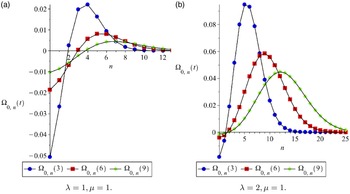
In Figure 1 this probability current is plotted as a function of n starting at $j=0$ for $t=3,6,9,$ and for a couple of values of the birth–death rates $\lambda,\mu$ . Note that the probability current is negative in the first states, since the state 0 can jump to the absorbing state $-1$ . If $\lambda>\mu$ (as in the figure on the right), the probability current is positive for large values of the states, since the boundary $+\infty$ is attracting.

Figure 1.

The probability current $\Omega_{0,n}(t)$ (10) is plotted as a function of n for $t = 3$ (blue circles), $t = 6$ (red squares), and $t =9$ (green diamonds) for a couple of values of the birth–death rates $\lambda,\mu$ .

We invite the reader to consult [Reference Ismail, Letessier, Masson and Valent18, Reference Karlin and McGregor22, Reference Karlin and McGregor21, Reference Parthasarathy and Lenin27, Reference Schoutens30] or more recently [Reference Domínguez de la Iglesia9, Chapter 3] for a compilation of examples.

2.2. State space $\mathbb{Z}$

Let $\{X_t \,:\, t\geq0\}$ be a birth–death process on $\mathbb{Z}$ with infinitesimal operator $\mathcal{A}$ given by the doubly infinite tridiagonal matrix

(11)

Now a diagram of the transitions between states is

These processes are also known as bilateral birth–death processes (following [Reference Pruitt29]), double-ended systems, or unrestricted birth–death processes (see [Reference Di Crescenzo, Iuliano and Martinucci6, Reference Di Crescenzo, Macci and Martinucci7, Reference Di Crescenzo and Martinucci8, Reference Giorno and Nobile13, Reference Giorno and Nobile14]). Again, we will assume that the set of rates $\{\lambda_n, \mu_n\}$ uniquely determines the bilateral birth–death process. In a similar way we can define the potential coefficients by

(12) \begin{equation}\pi_0=1,\quad\pi_n=\frac{\lambda_0\lambda_1\cdots \lambda_{n-1}}{\mu_1\mu_2\cdots \mu_n},\quad\pi_{-n}=\frac{\mu_0\mu_{-1}\cdots \mu_{-n+1}}{\lambda_{-1}\lambda_{-2}\cdots \lambda_{-n}},\quad n\in\mathbb{N}.\end{equation}

Again, these coefficients are defined as the solutions of the symmetry equations $\mathcal{A}_{ij}\pi_i=\mathcal{A}_{ji}\pi_j$ , $i,j\in\mathbb{Z},$ normalized by the condition $\pi_0=1$ (see [Reference Pruitt29, p. 510]), and are equivalent to $\pi_n\mu_n=\lambda_{n-1}\pi_{n-1}$ for $n\in\mathbb{Z}$ . If we assume that $\mathcal{A}$ is a closed, symmetric, self-adjoint, and negative operator in the Hilbert space $\ell^2_{\pi}(\mathbb{Z})$ , then, applying the spectral theorem (see [Reference Pruitt29]), we can obtain an integral representation of the transition probability functions $P_{ij}(t)=\mathbb{P}\!\left(X_t=j\,|\, X_0=i\right)$ in terms of three measures $\psi_{11}(x)$ , $\psi_{22}(x)$ , and $\psi_{12}(x)$ supported on $[0,\infty)$ and two linearly independent families of polynomials $(Q_n^{\alpha})_{n\in\mathbb{Z}}$ , $\alpha=1,2,$ generated by the three-term recurrence relations with initial conditions

(13) \begin{align}\nonumber Q_0^1(x)&=1,\quad Q_{0}^2(x)=0,\\Q_{-1}^1(x)&=0,\quad Q_{-1}^2(x)=1,\nonumber\\-xQ_n^{\alpha}(x)&=\lambda_nQ_{n+1}^{\alpha}(x)-(\lambda_n+\mu_n)Q_n^{\alpha}(x)+\mu_nQ_{n-1}^{\alpha}(x),\quad\alpha=1,2, \quad n\in\mathbb{Z}.\end{align}

This integral representation, called the Karlin–McGregor formula, is given by

(14) \begin{equation}P_{ij}(t)=\pi_j\int_{0}^{\infty}e^{-xt}\sum_{\alpha,\beta=1}^{2}Q_i^{\alpha}(x)Q_j^{\beta}(x)d\psi_{\alpha\beta}(x),\quad i,j\in\mathbb{Z}.\end{equation}

These three measures can be grouped in a positive definite $2\times2$ matrix, called the spectral matrix of the bilateral birth–death process:

(15) \begin{equation}\Psi(x)=\begin{pmatrix} \psi_{11}(x) & \quad \psi_{12}(x)\\[4pt] \psi_{12}(x) & \quad \psi_{22}(x) \end{pmatrix}.\end{equation}

Therefore, the Karlin–McGregor formula (14) can be written in matrix form as

(16) \begin{equation}P_{ij}(t)=\pi_j\int_{0}^{\infty}e^{-xt}\!\left(Q_i^1(x),Q_i^2(x)\right)d\Psi(x)\begin{pmatrix}Q_j^1(x)\\[6pt]Q_j^2(x)\end{pmatrix},\quad i,j\in\mathbb{Z}.\end{equation}

The computation of the measures $\psi_{\alpha\beta}(x)$ , $\alpha,\beta=1,2,$ can be reduced to the study of two birth–death processes on $\mathbb{N}_0$ corresponding to the two directions to infinity, with infinitesimal operators $\mathcal{A}_{ij}^+=\mathcal{A}_{ij}$ , $i,j\geq0$ , and $\mathcal{A}_{ij}^-=\mathcal{A}_{ij}$ , $i,j\leq-1$ , i.e.

(17) \begin{equation}\mathcal{A}^+=\begin{pmatrix}-(\lambda_0+\mu_0)& \quad \lambda_0&&&\\[3pt]\mu_1&\quad -(\lambda_1+\mu_1)&\quad \lambda_1&&\\[3pt]&\quad \mu_1&\quad -(\lambda_2+\mu_2)&\quad \lambda_2&\\[3pt]&&\quad \ddots&\quad \ddots&\quad \ddots\end{pmatrix}\end{equation}

and

(18) \begin{equation}\mathcal{A}^-=\begin{pmatrix}-(\lambda_{-1}+\mu_{-1})&\quad \mu_{-1}&&&\\[3pt]\lambda_{-2}&\quad -(\lambda_{-2}+\mu_{-2})&\quad \mu_{-2}&&\\[3pt]&\quad \lambda_{-3}&\quad -(\lambda_{-3}+\mu_{-3})&\quad \mu_{-3}&\\[3pt]&&\quad \ddots&\quad \ddots&\quad \ddots\end{pmatrix}.\end{equation}

Let us denote by $\psi^{\pm}$ the spectral measures associated with $\mathcal{A}^{\pm}$ (which are guaranteed by the spectral theorem applied to $\mathcal{A}^{\pm}$ ). The last section of [Reference Karlin and McGregor23] gives a method to relate the Stieltjes transforms of $\psi_{\alpha\beta}$ , $\alpha,\beta=1,2,$ in terms of the Stieltjes transforms of $\psi^{\pm}$ for discrete-time birth–death chains using probabilistic arguments. Here we will use the same arguments to derive similar relations (see Theorem 2.1 below). For that, let us call

\begin{equation*}F_{ij}(t)=\mathbb{P}\!\left(X_{\tau}=j\,\mbox{for some $\tau$}, 0<\tau\leq t\,|\,X_0=i\right), \quad i\neq j,\end{equation*}

the first passage time distributions and

\begin{equation*}F_{ii}(t)=\mathbb{P}\!\left(X_{\tau_1}\neq i, X_{\tau_2}=i\,\mbox{for some $\tau_1,\tau_2$}, 0<\tau_1<\tau_2\leq t\,|\,X_0=i\right),\end{equation*}

the recurrence time distributions. Let us denote by $\widehat{P}_{ij}(s)$ and $\widehat{F}_{ij}(s)$ the Laplace transforms of $P_{ij}(t)$ and $F_{ij}(t)$ , respectively; i.e.

(19) \begin{equation}\widehat{P}_{ij}(s)=\int_0^\infty e^{-st}P_{ij}(t)dt,\quad\widehat{F}_{ij}(s)=\int_0^\infty e^{-st}dF_{ij}(t),\quad i,j\in\mathbb{Z}.\end{equation}

We will use the same notation for the birth–death processes on $\mathbb{N}_0$ generated by $\mathcal{A}^{\pm}$ (i.e. $P_{ij}^{\pm}(t),F_{ij}^{\pm}(t)$ and $\widehat{P}_{ij}^{\pm}(s),\widehat{F}_{ij}^{\pm}(s)$ ). The Laplace transforms $\widehat{P}_{ij}(s)$ and $\widehat{F}_{ij}(s)$ are related by the following formulas (see [Reference Karlin and McGregor20, Reference Karlin and McGregor19]):

(20) \begin{equation}\begin{split}\widehat{P}_{ii}(s)&=\frac{1}{s+\lambda_i+\mu_i}+\widehat{P}_{ii}(s)\widehat{F}_{ij}(s),\\\widehat{P}_{ij}(s)&=\widehat{P}_{jj}(s)\widehat{F}_{ij}(s),\quad i\neq j.\end{split}\end{equation}

Theorem 2.1. Let $\psi_{\alpha\beta}$ , $\alpha,\beta=1,2,$ and $\psi^{\pm}$ be the spectral measures associated with $\mathcal{A}$ and $\mathcal{A}^{\pm}$ defined by (11), (17), and (18), respectively. Then we have the following relations:

(21) \begin{align}\nonumber B(z;\,\psi_{11})&=\frac{B(z;\,\psi^+)}{1-\lambda_{-1}\mu_0B(z;\,\psi^+)B(z;\,\psi^-)},\\\frac{\mu_0}{\lambda_{-1}}B(z;\,\psi_{22})&=\frac{B(z;\,\psi^-)}{1-\lambda_{-1}\mu_0B(z;\,\psi^+)B(z;\,\psi^-)},\end{align}

\begin{align}\nonumber B(z;\,\psi_{12})&=\frac{\lambda_{-1}B(z;\,\psi^+)B(z;\,\psi^-)}{1-\lambda_{-1}\mu_0B(z;\,\psi^+)B(z;\,\psi^-)},\end{align}

where $B(z;\,\psi)$ is the Stieltjes transform of $\psi$ defined by (6). In terms of the spectral matrix $\Psi$ (15) we have

(22) \begin{equation}B(z;\,\Psi)=\frac{B(z;\,\psi^+)B(z;\,\psi^-)}{1-\lambda_{-1}\mu_0B(z;\,\psi^+)B(z;\,\psi^-)}\begin{pmatrix} \displaystyle\frac{1}{B(z;\,\psi^-)} & \quad \lambda_{-1}\\[4pt] \lambda_{-1}& \quad \displaystyle\frac{\lambda_{-1}}{\mu_0B(z;\,\psi^+)}\end{pmatrix}.\end{equation}

Proof. From the identities

\begin{align*}\widehat{F}_{00}(s)&=\widehat{F}_{00}^+(s)+\frac{\mu_0}{s+\lambda_0+\mu_0}\widehat{F}_{-1,0}(s),\\\widehat{F}_{-1,0}(s)&=\lambda_{-1}\widehat{P}_{-1,-1}^-(s),\\\widehat{F}_{00}^+(s)&=1-\frac{1}{(s+\lambda_0+\mu_0)\widehat{P}_{00}^+(s)},\end{align*}

it is found that

(23) \begin{equation}\widehat{P}_{00}(s)=\frac{\widehat{P}_{00}^+(s)}{1-\lambda_{-1}\mu_0\widehat{P}_{00}^+(s)\widehat{P}_{-1,-1}^-(s)}.\end{equation}

Similarly, from the identities

\begin{align*}\widehat{F}_{-1,-1}(s)&=\widehat{F}_{-1,-1}^-(s)+\frac{\lambda_{-1}}{s+\lambda_{-1}+\mu_{-1}}\widehat{F}_{0,-1}(s),\\\widehat{F}_{0,-1}(s)&=\mu_{0}\widehat{P}_{00}^+(s),\\\widehat{F}_{-1,-1}^-(s)&=1-\frac{1}{(s+\lambda_{-1}+\mu_{-1})\widehat{P}_{-1,-1}^-(s)},\end{align*}

we obtain

(24) \begin{equation}\widehat{P}_{-1,-1}(s)=\frac{\widehat{P}_{-1,-1}^-(s)}{1-\lambda_{-1}\mu_0\widehat{P}_{00}^+(s)\widehat{P}_{-1,-1}^-(s)}.\end{equation}

Finally, $\widehat{P}_{-1,0}(s)=\widehat{P}_{00}(s)\widehat{F}_{-1,0}(s)$ gives

(25) \begin{equation}\widehat{P}_{-1,0}(s)=\frac{\lambda_{-1}\widehat{P}_{00}^+(s)\widehat{P}_{-1,-1}^-(s)}{1-\lambda_{-1}\mu_0\widehat{P}_{00}^+(s)\widehat{P}_{-1,-1}^-(s)}.\end{equation}

Now, using the Karlin–McGregor formula (14) in (19), we obtain

(26) \begin{equation}\widehat{P}_{ij}(s)=\pi_j\int_{0}^{\infty}\frac{1}{x+s}\sum_{\alpha,\beta=1}^{2}Q_i^{\alpha}(x)Q_j^{\beta}(x)d\psi_{\alpha\beta}(x)=\pi_jB\!\left({-}s;\,\sum_{\alpha,\beta=1}^{2}Q_i^{\alpha}Q_j^{\beta}\psi_{\alpha\beta}\right).\end{equation}

Similar formulas hold for $\widehat{P}_{ij}^{\pm}(s)$ with the measures $\psi^{\pm}$ . Therefore the formulas (23), (24), and (25) are equivalent to the Stieltjes transform relations (21).

As in the case of birth–death processes on $\mathbb{N}_0$ , we can derive some probabilistic properties of bilateral birth–death processes in terms of the spectral matrix. This was partially done in [Reference Pruitt28] for recurrence, limit theorems, and absorption probabilities, but for some reason it did not appear in [Reference Pruitt29]. Recently, since a bilateral birth–death process is a special case of a quasi-birth-and-death process with state space $\mathbb{N}_0\times\{1,2\}$ (see [Reference Kroese, Scheinhardt and Taylor24, Reference Latouche and Ramaswami25, Reference Neuts26] for more information about these processes), some other probabilistic properties have been derived in [Reference Dette and Reuther5].

Proposition 2.1. Let $\{X_t \,:\, t\geq0\}$ be a bilateral birth–death process with infinitesimal operator $\mathcal{A}$ (11). Then the the process is recurrent if and only if

(27) \begin{equation}\int_{0}^\infty\frac{\psi_{11}(x)}{x}dx=\infty \quad\mbox{or}\quad\pi_{-1}\int_{0}^\infty\frac{\psi_{22}(x)}{x}dx=\infty.\end{equation}

Moreover, the process is positive recurrent if and only if

(28) \begin{equation}{either}\quad \psi_{11}(x)\quad {or}\quad \pi_{-1}\psi_{22}(x)\quad {has\ a\ jump\ at\ the\ point}\ \textit{0}.\end{equation}

The size of this jump is the same for all measures and is given by

\begin{equation*}\psi(\{0\})=\left(\sum_{n\in\mathbb{Z}}\pi_n\right)^{-1}.\end{equation*}

Other quantities, such as the first moment of the first passage time distribution or limit theorems, can also be studied using the spectral matrix (see [Reference Pruitt28, Chapter 5] for more information).

Again, a fundamental role for bilateral birth–death processes is played by the probability current

(29) \begin{equation}\Omega_{j,n}(t)=\lambda_{n-1}P_{j,n-1}(t)-\mu_nP_{j,n}(t),\quad j,n\in\mathbb{Z},\end{equation}

which is related, as in the case of birth–death processes on $\mathbb{N}_0$ (see (5)), to the Kolmogorov forward equations

\begin{equation*}\frac{\partial}{\partial t}P_{j,n}(t)=\Omega_{j,n}(t)-\Omega_{j,n+1}(t),\quad j,n\in\mathbb{Z}.\end{equation*}

Using the Karlin–McGregor formula (14) and the symmetry property $\pi_n\mu_n=\lambda_{n-1}\pi_{n-1}$ , we can write $\Omega_{j,n}(t)$ as

(30) \begin{equation}\Omega_{j,n}(t)=\mu_n\pi_n\int_0^{\infty}e^{-xt}\sum_{\alpha,\beta=1}^2Q_j^\alpha(x)\left[Q_{n-1}^\beta(x)-Q_n^\beta(x)\right]d\psi_{\alpha\beta}(x),\quad j,n\in\mathbb{Z}.\end{equation}

Again, if we define the dual polynomials $(H_n^\alpha)_{n\in\mathbb{Z}}$ , $\alpha=1,2$ (see [Reference Pruitt28, Reference Pruitt29]), by

\begin{equation*}H_{n+1}^\alpha(x)=\lambda_n\pi_n\left[Q_{n+1}^\alpha(x)-Q_n^\alpha(x)\right],\quad \alpha=0,1,\quad n\in\mathbb{Z},\end{equation*}

then we can write $\Omega_{j,n}(t)$ as

\begin{equation*}\Omega_{j,n}(t)=-\int_0^{\infty}e^{-xt}\sum_{\alpha,\beta=1}^2Q_j^\alpha(x)H_n^\beta(x)d\psi_{\alpha\beta}(x),\quad j,n\in\mathbb{Z},\end{equation*}

and obtain a spectral representation of the probability current. We will use this spectral representation to plot the behavior of the probability current in several of the new examples we study in this paper.

As we pointed out in the introduction, there is only one explicit example of a bilateral birth–death process, as far as the author knows, where the spectral matrix and the corresponding orthogonal polynomials have been explicitly computed (see [Reference Ismail, Letessier, Masson and Valent18]). We will recall that example here, and we will also give another simple example motivated by the discrete-time random walk on $\mathbb{Z}$ with an attractive or repulsive force studied in [Reference Grünbaum15, Section 6] (see also [Reference De la Iglesia and Juarez4]).

In the next two examples and the new examples studied in Sections 3, 4, and 5, we will follow the same methodology in order to find the spectral matrix of the bilateral birth–death process and study its probabilistic properties. This methodology will be based on four steps:

1. 1. From the doubly infinite infinitesimal operator $\mathcal{A}$ (11) we consider the two semi-infinite infinitesimal operators $\mathcal{A^{\pm}}$ given in (17) and (18). We identify the Stieltjes transforms of the spectral measures $\psi^{\pm}$ associated with $\mathcal{A^{\pm}}$ using mainly Formula (7).

2. 2. We apply Theorem 2.1 to find the Stieltjes transform of the spectral matrix $\Psi$ (22). Once we have this function we use the Perron–Stieltjes inversion formula (see [Reference Dunford and Schwartz10, Theorem X.6.1] or [Reference Domínguez de la Iglesia9, Proposition 1.1]) to compute the spectral matrix $\Psi$ (15). In all the examples we study in this paper, the spectral matrix will be divided in an absolutely continuous part and a discrete part. The discrete part will be a collection of Dirac deltas located at the poles of the Stieltjes transform of the spectral matrix, whenever they exist.

3. 3. We identify the corresponding orthogonal polynomials $(Q_n^{\alpha})_{n\in\mathbb{Z}}$ , $\alpha=1,2,$ by looking at the three-term recurrence relation (13). All the examples we study in this paper are related somehow to the Chebyshev polynomials of the first and second kind. Using these polynomials we obtain the Karlin–McGregor formula (14) or (16) for the transition probability functions $P_{ij}(t)$ .

4. 4. We study recurrence of the bilateral birth–death process using Proposition 2.2, give the invariant distribution (whenever it exists), and display some plots of the probability current $\Omega_{0,n}(t)$ using the integral representation (30).

Example 2.2. Bilateral birth–death process with constant rates [Reference Ismail, Letessier, Masson and Valent18]. Consider the bilateral birth–death process with constant birth–death rates

\begin{equation*}\lambda_n=\lambda,\quad\mu_n=\mu,\quad n\in\mathbb{Z},\quad\lambda,\mu>0.\end{equation*}

The matrix $\mathcal{A}^+$ in (17) is the same as the one for the absorbing M/M/1 queue in Example 2.1, while $\mathcal{A}^-$ in (18) is the symmetric matrix of $\mathcal{A}^+$ . Therefore both processes generate the same Stieltjes transform, given by (8). Following (21) we obtain that

\begin{align*}B(z;\,\psi_{11})&=\frac{\mu}{\lambda}B(z;\,\psi_{22})=\frac{1}{\sqrt{(\lambda+\mu-z)^2-4\lambda\mu}},\\[3pt]B(z;\,\psi_{12})&=\frac{1}{2\mu}\!\left({-}1+\frac{\lambda+\mu-z}{\sqrt{(\lambda+\mu-z)^2-4\lambda\mu}}\right).\end{align*}

Observe that the jumps, if any, should be located at $x=\sigma_{\pm}$ where $\sigma_{\pm}=\big(\sqrt{\lambda}\pm\sqrt{\mu}\big)^2$ . However, it follows easily that the size of these jumps must be 0, so there are no jumps. The spectral matrix is then given by

\begin{equation*}\Psi(x)=\frac{1}{\pi\sqrt{(x-\sigma_-)(\sigma_+-x)}}\begin{pmatrix}1&\quad (\lambda+\mu-x)/2\mu\\[4pt](\lambda+\mu-x)/2\mu&\quad \lambda/\mu\end{pmatrix},\quad x\in[\sigma_-,\sigma_+].\end{equation*}

The polynomials generated by the three-term recurrence relation (13) (something that was not pointed out in [Reference Ismail, Letessier, Masson and Valent18]) are given by

\begin{align*}Q_n^1(x)&=\left(\frac{\mu}{\lambda}\right)^{n/2}U_n\!\left(\frac{\lambda+\mu-x}{2\sqrt{\lambda\mu}}\right),\!\!\quad Q_{-n-1}^1(x)=-\!\left(\frac{\lambda}{\mu}\right)^{(n+1)/2}U_{n-1}\!\left(\frac{\lambda+\mu-x}{2\sqrt{\lambda\mu}}\right),\!\!\quad n\in\mathbb{N}_0,\\Q_n^2(x)&=-\!\left(\frac{\mu}{\lambda}\right)^{(n+1)/2}U_{n-1}\!\left(\frac{\lambda+\mu-x}{2\sqrt{\lambda\mu}}\right),\!\!\quad Q_{-n-1}^2(x)=\left(\frac{\lambda}{\mu}\right)^{n/2}U_{n}\!\left(\frac{\lambda+\mu-x}{2\sqrt{\lambda\mu}}\right),\!\!\quad n\in\mathbb{N}_0,\end{align*}

where again $(U_n)_{n\in\mathbb{N}_0}$ are the Chebyshev polynomials of the second kind. The transition probability functions $P_{ij}(t)$ can then be approximated using the Karlin–McGregor formula (14). In this case the transition probability functions were explicitly computed in [Reference Conolly3] and are given by

\begin{equation*}P_{ij}(t)=e^{-(\lambda+\mu)t}\!\left(\sqrt{\frac{\lambda}{\mu}}\right)^{j-i}I_{j-i}\!\left(2\sqrt{\lambda\mu}t\right),\quad i,j\in\mathbb{Z},\end{equation*}

where again $I_\nu(z)$ denotes the modified Bessel function of the first kind. The previous formula can also be derived using basic properties of Chebyshev polynomials in the Karlin–McGregor formula (14).

From the spectral matrix it is possible to see that $\int_0^\infty x^{-1}\psi_{11}(x)dx<\infty$ and $\int_0^\infty x^{-1}\psi_{22}(x)dx<\infty$ unless $\lambda=\mu$ , where both integrals diverge. Therefore, from Proposition 2.2, if $\lambda\neq\mu$ the process is transient. If $\lambda=\mu$ the process is null recurrent, since the measure does not have a jump at $x=0$ . Finally, since we have an explicit expression for $P_{ij}(t)$ , we have that the probability current (29) is given by

\begin{equation*}\Omega_{j,n}(t)=\mu e^{-(\lambda+\mu)t}\!\left(\sqrt{\frac{\lambda}{\mu}}\right)^{n-j}\!\left(\sqrt{\lambda/\mu}I_{n-j-1}(2\sqrt{\lambda\mu}t)-I_{n-j}(2\sqrt{\lambda\mu}t)\right),\quad j,n\in\mathbb{Z}.\end{equation*}

Some plots of $\Omega_{0,n}(t)$ can be found in [Reference Giorno and Nobile13, Figure 9].

Example 2.3. Symmetric bilateral birth–death process with constant rates. Consider the bilateral birth–death process with birth–death rates

\begin{equation*}\lambda_n=\lambda,\quad\mu_n=\mu, \quad n\in\mathbb{N}_0,\quad \lambda_{-n}=\mu,\quad \mu_{-n}=\lambda, \quad n\in\mathbb{N},\quad \lambda,\mu>0.\end{equation*}

The matrices $\mathcal{A}^{\pm}$ in (17) and (18) are equal and the same as the one for the absorbing M/M/1 queue in Example 2.1. Therefore the corresponding Stieltjes transforms are given by (8). Following (21) and rationalizing, we obtain that

\begin{align*}B(z;\,\psi_{11})&=B(z;\,\psi_{22})=\frac{(\lambda-\mu)(\lambda+\mu-z)-(\lambda+\mu)\sqrt{(\lambda+\mu-z)^2-4\lambda\mu}}{2\mu z(2\lambda+2\mu-z)},\\[4pt]B(z;\,\psi_{12})&=\frac{\mu(\mu+2z)-(\lambda-z)^2+(\lambda+\mu-z)\sqrt{(\lambda+\mu-z)^2-4\lambda\mu}}{2\mu z(2\lambda+2\mu-z)}.\end{align*}

The spectral matrix $\Psi(x)=\Psi_c(x)+\Psi_d(x)$ has now an absolutely continuous part $\Psi_c(x)$ , given by

\begin{equation*}\Psi_c(x)=\frac{\sqrt{(x-\sigma_-)(\sigma_+-x)}}{2{\pi}\mu x(2\lambda+2\mu-x)}\begin{pmatrix}\lambda+\mu& \quad \lambda+\mu-x\\[4pt]\lambda+\mu-x& \quad \lambda+\mu\end{pmatrix},\quad x\in[\sigma_-,\sigma_+],\end{equation*}

where $\sigma_{\pm}=\big(\sqrt{\lambda}\pm\sqrt{\mu}\big)^2$ , and a discrete part $\Psi_d(x)$ , given by

\begin{equation*}\Psi_d(x)=\frac{\mu-\lambda}{2\mu}\left[\begin{pmatrix}1&\quad 1\\[3pt]1& \quad 1\end{pmatrix}\delta_0(x)+\begin{pmatrix}1&\quad -1\\[3pt]-1&\quad 1\end{pmatrix}\delta_{2\lambda+2\mu}(x)\right]\mathbf{1}_{\{\mu>\lambda\}},\end{equation*}

where $\mathbf{1}_A$ is the indicator function and $\delta_a(x)$ is the Dirac delta located at $x=a$ . The polynomials generated by the three-term recurrence relation (13) are given by

\begin{align*}Q_n^1(x)&=\left(\frac{\mu}{\lambda}\right)^{n/2}U_n\!\left(\frac{\lambda+\mu-x}{2\sqrt{\lambda\mu}}\right),\!\!\quad Q_{-n-1}^1(x)=-\!\left(\frac{\mu}{\lambda}\right)^{(n+1)/2}U_{n-1}\!\left(\frac{\lambda+\mu-x}{2\sqrt{\lambda\mu}}\right),\!\!\quad n\in\mathbb{N}_0,\\[3pt]Q_n^2(x)&=-\!\left(\frac{\mu}{\lambda}\right)^{(n+1)/2}U_{n-1}\!\left(\frac{\lambda+\mu-x}{2\sqrt{\lambda\mu}}\right),\!\!\quad Q_{-n-1}^2(x)=\left(\frac{\mu}{\lambda}\right)^{n/2}U_{n}\!\left(\frac{\lambda+\mu-x}{2\sqrt{\lambda\mu}}\right),\!\!\quad n\in\mathbb{N}_0,\end{align*}

where again $(U_n)_{n\in\mathbb{N}_0}$ are the Chebyshev polynomials of the second kind. The transition probability functions $P_{ij}(t)$ can then be approximated using the Karlin–McGregor formula (14). Unlike in the previous example, no explicit formula for $P_{ij}(t)$ has been found in terms of Bessel functions, as far as the author knows.

Following (27), from the spectral matrix it is possible to see that if $\lambda>\mu$ then $\int_0^\infty x^{-1}\psi_{11}(x)dx<\infty$ and $\int_0^\infty x^{-1}\psi_{22}(x)dx<\infty$ . This is because the point $x=0$ never belongs to the support of the spectral matrix. Therefore, if $\lambda>\mu$ the process is transient. Otherwise, if $\lambda\leq\mu$ , both integrals diverge because the point $x=0$ belongs to the support of the spectral matrix, either if we have a discrete Dirac delta at $x=0$ (for $\lambda<\mu$ ) or the absolutely continuous support reaches $x=0$ (for $\lambda=\mu$ ). Therefore, if $\lambda\leq\mu$ the process is recurrent. Following (28), if $\lambda<\mu$ , both measures $\psi_{11},\psi_{22}$ will always have a jump at the point 0. Therefore it will be positive recurrent. If $\lambda=\mu$ then the process will be null recurrent. Since the potential coefficients are given here (see (12)) by

\begin{equation*}\pi_n=\left(\frac{\lambda}{\mu}\right)^{n},\quad \pi_{-n-1}=\left(\frac{\lambda}{\mu}\right)^{n},\quad n\in\mathbb{N}_0,\end{equation*}

we have that the invariant distribution $\boldsymbol\pi$ for this process is given by

\begin{equation*}\boldsymbol\pi=\frac{\mu-\lambda}{2\mu}\!\left(\cdots,\frac{\lambda}{\mu},1,1,\frac{\lambda}{\mu},\frac{\lambda^2}{\mu^2},\cdots\right),\quad \mu>\lambda.\end{equation*}

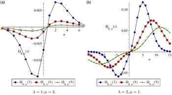
Now we do not have an explicit expression for the transition probability functions, so we also do not have an explicit expression for the probability current $\Omega_{j,n}(t)$ (29). Nevertheless we can get an approximation using (30), the spectral matrix, and the corresponding orthogonal polynomials. In Figure 2 this probability current is plotted as a function of n starting at $j=0$ for $t=3,6,9,$ and for a couple of values of the birth–death rates $\lambda,\mu$ . Note that for $\lambda<\mu$ the endpoints $\pm\infty$ are reflecting boundaries, but if $\lambda>\mu$ the probability current shifts to the left if $n < 0$ and to the right for $n > 0$ as t increases, since $\pm\infty$ are absorbing boundaries.

Figure 2.

The probability current $\Omega_{0,n}(t)$ (30) for Example 2.3 is plotted as a function of n for $t = 3$ (blue circles), $t = 6$ (red squares), and $t =9$ (green diamonds) for a couple of values of the birth–death rates $\lambda,\mu$ .

3.1. Case 1

Consider the bilateral birth–death process with birth–death rates given by

\begin{equation*}\lambda_{2n}=\lambda,\quad\lambda_{2n+1}=\mu, \quad \mu_{2n}=\lambda,\quad \mu_{2n+1}=\mu, \quad n\in\mathbb{Z},\quad \lambda,\mu>0.\end{equation*}

The matrices $\mathcal{A}^{\pm}$ in (17) and (18) are now given by

\begin{equation*}\mathcal{A}^+=\begin{pmatrix}-2\lambda& \quad \lambda& \quad & \quad & \quad \\[3pt]\mu& \quad -2\mu& \quad \mu& \quad & \quad \\[3pt]& \quad \lambda& \quad -2\lambda& \quad \lambda& \quad \\[3pt]& \quad & \quad \ddots& \quad \ddots& \quad \ddots\end{pmatrix},\quad\mathcal{A}^-=\begin{pmatrix}-2\mu& \quad \mu& \quad & \quad & \quad \\[3pt]\lambda& \quad -2\lambda& \quad \lambda& \quad & \quad \\[3pt]& \quad \mu& \quad -2\mu& \quad \mu& \quad \\[3pt]& \quad & \quad \ddots& \quad \ddots& \quad \ddots\end{pmatrix}.\end{equation*}

Observe that $\mathcal{A}^-$ is the infinitesimal operator of the 0th birth–death process on $\mathbb{N}_0$ associated to $\mathcal{A}^+$ (i.e. the infinitesimal operator defined from $\mathcal{A^+}$ by eliminating the first row and column of $\mathcal{A^+}$ ). Also, $\mathcal{A}^-$ is the same matrix as $\mathcal{A}^+$ except with $\lambda$ replaced by $\mu$ . Applying (7) twice, we obtain the following algebraic relation satisfied by the Stieltjes transform of the measure $\psi^+$ associated with $\mathcal{A}^+$ :

\begin{equation*}\lambda\mu(z-2\lambda)B^2(z;\,\psi^+)+(2\lambda-z)(2\mu-z)B(z;\,\psi^+)+z-2\lambda=0.\end{equation*}

Solving, we obtain

\begin{equation*}B(z;\,\psi^+)=\frac{1}{2\lambda\mu}\!\left(2\mu-z-\sqrt{-\frac{z(2\mu-z)(2\lambda+2\mu-z)}{2\lambda-z}}\right).\end{equation*}

If $\lambda\neq\mu$ the expression inside the square root is negative only for

(31) \begin{equation}z\in J_1=[0,2\lambda\wedge2\mu]\quad\mbox{or}\quad z\in J_2=[2\lambda\vee2\mu,2\lambda+2\mu],\end{equation}

where, as usual, $a\wedge b=\min\{a,b\}$ and $a\vee b=\max\{a,b\}$ . It is also possible to see that there are no jumps. Therefore the spectral measure is given by

\begin{equation*}\psi^+(x)=\frac{1}{2\pi\lambda\mu}\sqrt{\frac{x(2\mu-x)(2\lambda+2\mu-x)}{2\lambda-x}},\quad x\in J_1\cup J_2.\end{equation*}

The spectral measure for $\psi^-$ is the same but with $\lambda$ replaced by $\mu$ . Observe that if $\lambda=\mu$ we go back to the spectral measure of the absorbing M/M/1 queue in (9).

Now, going back to the bilateral birth–death process and using the algebraic properties of $B(z;\,\psi^{\pm})$ , we have, following (21) and after rationalizing, that

\begin{align*}B(z;\,\psi_{11})&=-\sqrt{-\frac{2\mu-z}{z(2\lambda-z)(2\lambda+2\mu-z)}},\\[3pt]B(z;\,\psi_{12})&=-\frac{1}{2\lambda}\!\left(1+\sqrt{-\frac{(2\lambda-z)(2\mu-z)}{z(2\lambda+2\mu-z)}}\right),\\[3pt]B(z;\,\psi_{22})&=-\frac{\mu}{\lambda}\sqrt{-\frac{2\lambda-z}{z(2\mu-z)(2\lambda+2\mu-z)}}.\end{align*}

Again, it is possible to see that there are no jumps. Therefore the spectral matrix has only an absolutely continuous part, given by

\begin{equation*}\Psi(x)=\frac{1}{\pi}\begin{pmatrix} \displaystyle\sqrt{\frac{2\mu-x}{x(2\lambda-x)(2\lambda+2\mu-x)}}& \quad \displaystyle\frac{1}{2\lambda}\sqrt{\frac{(2\lambda-x)(2\mu-x)}{x(2\lambda+2\mu-x)}}\\[17pt] \displaystyle\frac{1}{2\lambda}\sqrt{\frac{(2\lambda-x)(2\mu-x)}{x(2\lambda+2\mu-x)}}& \quad \displaystyle\frac{\mu}{\lambda}\sqrt{\frac{2\lambda-x}{x(2\mu-x)(2\lambda+2\mu-x)}}\end{pmatrix},\quad x\in J_1\cup J_2.\end{equation*}

The explicit expression for the polynomials is now more difficult to compute. But using the main theorem in [Reference Beckermann, Gilewicz and Leopold1] it is possible to obtain an explicit expression for the polynomials generated by the three-term recurrence relation (13). If we define the new variable

\begin{equation*}y=-1+\frac{(2\lambda-x)(2\mu-x)}{2\lambda\mu},\end{equation*}

then for the first family we have

\begin{align*}Q_{2k}^1(x)&=(2y+1)U_{k-1}(y)-U_{k-2}(y),\!\quad k\in\mathbb{N},\!\quad Q_{2k+1}^1(x)=-\frac{1}{\lambda}(x-2\lambda)U_{k}(y),\!\quad k\in\mathbb{N}_0,\\Q_{-2k-2}^1(x)&=-(2y+1)U_{k-1}(y)+U_{k-2}(y),\!\!\!\quad k\in\mathbb{N}_0,\!\!\!\quad Q_{-2k-1}^1(x)=\frac{1}{\lambda}(x-2\lambda)U_{k-1}(y),\!\!\!\quad k\in\mathbb{N},\end{align*}

and for the second family we have $Q_1^2(x)=-1$ and

\begin{align*}Q_{2k}^2(x)&=\frac{1}{\mu}(x-2\mu)U_{k-1}(y),\!\quad k\in\mathbb{N}_0,\!\quad Q_{2k+1}^2(x)=-(2y+1)U_{k-1}(y)+U_{k-2}(y),\!\quad k\in\mathbb{N},\\Q_{-2k}^2(x)&=-\frac{1}{\mu}(x-2\mu)U_{k-1}(y),\!\quad k\in\mathbb{N}_0,\!\!\quad Q_{-2k-1}^2(x)=(2y+1)U_{k-1}(y)-U_{k-2}(y),\!\!\!\quad k\in\mathbb{N},\end{align*}

where again $(U_n)_{n\in\mathbb{N}_0}$ are the Chebyshev polynomials of the second kind. The transition probability functions $P_{ij}(t)$ can then be approximated using the Karlin–McGregor formula (14).

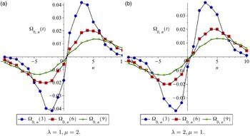
From (27) and the explicit expression for the spectral matrix, we have that $\int_0^\infty x^{-1}\psi_{11}(x)dx=\int_0^\infty x^{-1}\psi_{22}(x)dx=\infty$ for any values of $\lambda,\mu$ . Therefore the process is always recurrent, as expected. Since there is no jump at the point 0, the process is always null recurrent. Again, we can get an approximation of the probability current by using (30), the spectral matrix, and the corresponding orthogonal polynomials. In Figure 3 this probability current is plotted as a function of n starting at $j=0$ for $t=3,6,9,$ and for a couple values of the birth–death rates $\lambda,\mu$ .

Figure 3.

The probability current $\Omega_{0,n}(t)$ (30) for the example in Section 3.1 is plotted as a function of n for $t = 3$ (blue circles), $t = 6$ (red squares), and $t =9$ (green diamonds) for a couple of values of the birth–death rates $\lambda,\mu$ .

3.2. Case 2

Consider the bilateral birth–death process with birth–death rates given by

\begin{equation*}\lambda_{2n}=\lambda,\quad\lambda_{2n+1}=\mu, \quad \mu_{2n}=\mu,\quad \mu_{2n+1}=\lambda, \quad n\in\mathbb{Z},\quad \lambda,\mu>0.\end{equation*}

The matrices $\mathcal{A}^{\pm}$ in (17) and (18) are now given by

\begin{equation*}\mathcal{A}^+=\mathcal{A}^-=\begin{pmatrix}-(\lambda+\mu)& \quad \lambda& \quad & \quad & \quad \\[3pt]\lambda& \quad -(\lambda+\mu)& \quad \mu& \quad & \quad \\[3pt]& \quad \mu& \quad -(\lambda+\mu)& \quad \lambda& \quad \\[3pt]& \quad & \quad \ddots& \quad \ddots& \quad \ddots\end{pmatrix}.\end{equation*}

Applying (7) twice, we obtain the following expression for the the Stieltjes transform of the measure $\psi^+$ :

\begin{equation*}B(z;\,\psi^+)=\frac{z^2-2(\lambda+\mu)z+2\mu(\lambda+\mu)-\sqrt{-z(2\mu-z)(2\lambda-z)(2\lambda+2\mu-z)}}{2\mu^2(\lambda+\mu-z)}.\end{equation*}

Now $\psi^+$ will have an absolutely continuous part and a discrete part. Indeed

\begin{equation*}\psi^+(x)=\frac{\sqrt{x(2\lambda-x)(2\mu-x)(2\lambda+2\mu-x)}}{2\pi\mu^2|\lambda+\mu-x|}\mathbf{1}_{\{J_1\cup J_2\}},+\left(1-\frac{\lambda^2}{\mu^2}\right)\delta_{\lambda+\mu}(x)\mathbf{1}_{\{\mu>\lambda\}},\end{equation*}

where $\mathbf{1}_A$ is the indicator function, $\delta_a(x)$ is the Dirac delta located at $x=a$ , and $J_1,J_2$ are defined by (31). Now, going back to the bilateral birth–death process and using the algebraic properties of $B(z;\,\psi^{+})=B(z;\,\psi^{-})$ , we have, following (21) and after rationalizing, that

\begin{align*}B(z;\,\psi_{11})&=B(z;\,\psi_{22})=-\frac{\lambda+\mu-z}{\sqrt{-z(2\mu-z)(2\lambda-z)(2\lambda+2\mu-z)}},\\[5pt]B(z;\,\psi_{12})&=-\frac{1}{2\mu}\!\left(1+\frac{(\lambda+\mu-z)^2+\mu^2-\lambda^2}{\sqrt{-z(2\mu-z)(2\lambda-z)(2\lambda+2\mu-z)}}\right),\end{align*}

Again, it is possible to see that there are no jumps. Therefore the spectral matrix has only an absolutely continuous part, given by

\begin{align*}\Psi(x) & =\frac{1}{\pi\sqrt{x(2\mu-x)(2\lambda-x)(2\lambda+2\mu-x)}}\nonumber\\[5pt]& \quad \times \begin{pmatrix} |\lambda+\mu-x|& \quad |(\lambda+\mu-x)^2+\mu^2-\lambda^2|\\[6pt] |(\lambda+\mu-x)^2+\mu^2-\lambda^2|& \quad |\lambda+\mu-x|\end{pmatrix},\end{align*}

where $x\in J_1\cup J_2$ and $J_1,J_2$ are defined by (31). Again, by using the main theorem in [Reference Beckermann, Gilewicz and Leopold1], it is possible to obtain an explicit expression for the polynomials generated by the three-term recurrence relation (13). If we define the new variable

\begin{equation*}y=\frac{(\lambda+\mu-x)^2-\lambda^2-\mu^2}{2\lambda\mu},\end{equation*}

then we have $Q_1^2(x)=-\mu/\lambda$ and

\begin{align*}Q_{2k}^1(x)&=(2y+\mu/\lambda)U_{k-1}(y)-U_{k-2}(y),\quad k\in\mathbb{N},\quad Q_{2k+1}^1(x)=\frac{1}{\lambda}(\lambda+\mu-x)U_{k}(y),\quad k\in\mathbb{N}_0,\\Q_{2k}^2(x)&=\frac{1}{\lambda}(x-\lambda-\mu)U_{k-1}(y),\quad k\in\mathbb{N}_0,\quad Q_{2k+1}^2(x)=-\frac{\mu}{\lambda}\left[(2y+\lambda/\mu)U_{k-1}(y)-U_{k-2}(y)\right],\quad k\in\mathbb{N},\end{align*}

while for the negative indices we have $Q_{-n-1}^1(x)=Q_n^2(x)$ and $Q_{-n-1}^2(x)=Q_n^1(x)$ for $n\in\mathbb{N}_0$ . Again $(U_n)_{n\in\mathbb{N}_0}$ are the Chebyshev polynomials of the second kind. The transition probability functions $P_{ij}(t)$ can then be approximated using the Karlin–McGregor formula (14). The probabilistic properties of this process are the same as in the previous case; i.e. the process is always null recurrent. Also, graphs of the probability current are similar to the ones plotted in Figure 3.

4.1. Case 1

The birth–death rates are now given by

\begin{equation*}\lambda_n=\lambda,\quad\mu_n=\mu,\quad n\in\mathbb{Z}\setminus\{0\},\quad\lambda,\mu,\lambda_0,\mu_0>0.\end{equation*}

Now the matrix $\mathcal{A}^+$ in (17) is given by

\begin{equation*}\mathcal{A}^+=\begin{pmatrix}-(\lambda_0+\mu_0)& \quad \lambda_0& \quad & \quad & \quad \\[3pt]\mu& \quad -(\lambda+\mu)& \quad \lambda& \quad & \quad \\[3pt]& \quad \mu& \quad -(\lambda+\mu)& \quad \lambda& \quad \\[3pt]& & \quad \ddots& \quad \ddots& \quad \ddots\end{pmatrix},\end{equation*}

while the matrix $\mathcal{A}^-$ in (18) is the same as the one for the absorbing M/M/1 queue in Example 2.1 and also the infinitesimal operator of the 0th birth–death process associated to $\mathcal{A}^+$ (i.e. the infinitesimal operator defined from $\mathcal{A^+}$ by eliminating the first row and column of $\mathcal{A^+}$ ). Calling B(z) the Stieltjes transform in (8) and applying (7), we obtain

(32) \begin{equation}B(z;\,\psi^+)=\frac{1}{\lambda_0+\mu_0-z-\lambda_0\mu B(z)},\quad B(z;\,\psi^-)=B(z).\end{equation}

Following (21) and rationalizing, we obtain that

\begin{equation*}B(z;\,\psi_{\alpha\beta})=\frac{p_{\alpha\beta}(z)+q_{\alpha\beta}(z)\sqrt{(\lambda+\mu-z)^2-4\lambda\mu}}{D(z)},\quad \alpha,\beta=1,2,\end{equation*}

where

\begin{align*}p_{11}(z)&=(\lambda_0\mu+\mu_0\lambda-2\lambda\mu)z+(\lambda-\mu)(\lambda_0\mu-\mu_0\lambda),\quad q_{11}(z)=-(\lambda_0\mu+\lambda\mu_0),\\p_{12}(z)&=\lambda\left[z^2-(\lambda_0+\mu_0+\lambda+\mu)z+(\lambda - \mu)(\lambda_0 - \mu_0)\right],\quad q_{12}(z)=-\lambda(\lambda_0+\mu_0-z),\\p_{22}(z)&=\frac{1}{\mu_0}\left[(\lambda_0 - \lambda)z^3+\big({-}\lambda_0^2 - \lambda_0\mu_0 - 2\lambda_0\mu + 2\mu_0\lambda + \lambda^2 + \lambda\mu\big)z^2\right.\\& \quad\qquad +\mu_0(\lambda - \mu)(\lambda_0\mu - \mu_0\lambda)\\&\quad\qquad \left.+\big(\lambda_0^2\lambda + \lambda_0^2\mu - \lambda_0\mu_0\lambda + 2\lambda_0\mu_0\mu - \lambda_0\lambda^2 + \lambda_0\mu^2 - \mu_0^2\lambda - 2\mu_0\lambda\mu\big)z\right],\\q_{22}(z)&=-\frac{1}{\mu_0}\left[(\lambda-\lambda_0)z^2+\big(\lambda_0^2 + \lambda_0\mu_0 - \lambda_0\lambda + \lambda_0\mu - 2\mu_0\lambda\big)z+\mu_0(2\lambda_0\lambda - \lambda_0\mu + \mu_0\lambda)\right],\\D(z)&=\big({-}2\lambda_0\mu-2\mu_0\lambda+2\lambda\mu\big)z^2-2\lambda_0\mu_0(\lambda - \mu)^2\\&\qquad +\big(2\lambda_0^2\mu + 2\lambda_0\mu_0\lambda + 2\lambda_0\mu_0\mu - 2\lambda_0\lambda\mu + 2\lambda_0\mu^2 + 2\mu_0^2\lambda + 2\mu_0\lambda^2 - 2\mu_0\lambda\mu\big)z.\end{align*}

The spectral matrix $\Psi(x)=\Psi_c(x)+\Psi_d(x)$ has now an absolutely continuous part $\Psi_c(x)$ , given by

\begin{equation*}\Psi_c(x)=\frac{\sqrt{(x-\sigma_-)(\sigma_+-x)}}{\pi D(x)}\begin{pmatrix}\lambda_0\mu+\lambda\mu_0& \quad \lambda(\lambda_0+\mu_0-x)\\[5pt]\lambda(\lambda_0+\mu_0-x)&\quad q_{22}(x)\end{pmatrix},\quad x\in[\sigma_-,\sigma_+],\end{equation*}

where $\sigma_{\pm}=\big(\sqrt{\lambda}\pm\sqrt{\mu}\big)^2$ . For the discrete part $\Psi_d(x)$ we need to study the poles of $B(z;\,\psi_{\alpha\beta})$ , $\alpha,\beta=1,2,$ which are the roots of the second-degree polynomial D(z). For that, let us introduce some constants which will considerably simplify the sequel:

\begin{align*}R&=(\lambda_0 - \mu_0 - \lambda + \mu)^2 + 4\lambda_0\mu_0,\\[3pt]C&=\lambda\mu R-(\lambda_0\mu+\mu_0\lambda-\lambda\mu)(\lambda_0\mu+\mu_0\lambda+2\lambda\mu).\end{align*}

The roots of D(z) are then given by

(33) \begin{equation}\gamma_{\pm}=\frac{(\lambda_0\mu + \mu_0\lambda)(\lambda_0 + \mu_0) + (\lambda_0\mu - \mu_0\lambda)(\mu-\lambda)\pm (\lambda_0\mu + \mu_0\lambda)\sqrt{R}}{2(\lambda_0\mu + \mu_0\lambda - \lambda\mu)}.\end{equation}

Observe that $\sqrt{R}$ is well-defined since $R>0$ . A long but straightforward computation gives the magnitude for each of these poles. Defining the constants

\begin{align*}A_{11}^{\pm}&=\frac{1}{2(\lambda_0\mu+\mu_0\lambda-\lambda\mu)}\left[\lambda_0\mu+\mu_0\lambda-2\lambda\mu\pm(\lambda_0\mu+\mu_0\lambda)(\lambda+\mu-\lambda_0-\mu_0)\frac{\sqrt{R}}{R}\right],\\A_{12}^{\pm}&=\frac{\lambda}{2(\lambda_0\mu+\mu_0\lambda-\lambda\mu)^2}\left[\lambda\mu(\lambda+\mu-\lambda_0-\mu_0)\right.\\& \quad\left.\pm(C-(\lambda_0\mu+\mu_0\lambda-\lambda\mu)(\lambda_0\mu+\mu_0\lambda-2\lambda\mu))\frac{\sqrt{R}}{R}\right],\\A_{22}^{\pm}&=\frac{\lambda^2}{2(\lambda_0\mu+\mu_0\lambda-\lambda\mu)^3}\left[-C\pm(\lambda+\mu-\lambda_0-\mu_0)(C+2\lambda\mu(\lambda_0\mu+\mu_0\lambda-\lambda\mu))\frac{\sqrt{R}}{R}\right],\end{align*}

we have that the discrete part $\Psi_d(x)$ is given by

\begin{equation*}\Psi_d(x)=\begin{pmatrix}A_{11}^-& \quad A_{12}^-\\[6pt]A_{12}^-&\quad A_{22}^-\end{pmatrix}\delta_{\gamma_+}(x)\mathbf{1}_{\{A_{11}^->0,\gamma_+>0\}}+\begin{pmatrix}A_{11}^+&\quad A_{12}^+\\[6pt]A_{12}^+&\quad A_{22}^+\end{pmatrix}\delta_{\gamma_-}(x)\mathbf{1}_{\{A_{11}^+>0,\gamma_->0\}},\end{equation*}

where $\mathbf{1}_A$ is the indicator function and $\delta_a(x)$ is the Dirac delta located at $x=a$ . We have not been able to find a simplification of the conditions $\{A_{11}^->0,\gamma_+>0\}$ and $\{A_{11}^+>0,\gamma_->0\}$ in terms of the birth–death rates $\lambda,\mu,\lambda_0,\mu_0$ . Finally, we can also compute the polynomials generated by the three-term recurrence relation (13). If we define the new variable

(34) \begin{equation}y=\frac{\lambda+\mu-x}{2\sqrt{\lambda\mu}},\end{equation}

then we have

(35) \begin{align} Q_n^1(x)&=\left(\frac{\mu}{\lambda}\right)^{n/2}\left[\frac{2(\lambda_0-\lambda)}{\lambda_0}T_n\left(y\right)+\frac{2\lambda-\lambda_0}{\lambda_0}U_n\left(y\right)\right.\nonumber\\& \qquad\qquad\qquad \left. +\sqrt{\frac{\lambda}{\mu}}\frac{\lambda_0+\mu_0-\lambda-\mu}{\lambda_0}U_{n-1}\!\left(y\right)\right],\quad n\in\mathbb{N}_0,\nonumber\\Q_{-n-1}^1(x)&=-\left(\frac{\lambda}{\mu}\right)^{(n+1)/2}U_{n-1}\!\left(y\right),\quad n\in\mathbb{N}_0,\\Q_n^2(x)&=-\frac{\mu_0}{\lambda_0}\!\left(\frac{\mu}{\lambda}\right)^{(n-1)/2}U_{n-1}\!\left(y\right),\quad Q_{-n-1}^2(x)=\left(\frac{\lambda}{\mu}\right)^{n/2}U_{n}\!\left(y\right),\quad n\in\mathbb{N}_0,\nonumber\end{align}

where $(T_n)_{n\in\mathbb{N}_0}$ and $(U_n)_{n\in\mathbb{N}_0}$ are the Chebyshev polynomials of the first and second kind, respectively.

Remark 4.1. The polynomials $\big(Q_n^1\big)_{n\in\mathbb{N}_0}$ in (35) can be written in terms of perturbed Chebyshev polynomials (see [Reference Chihara2, pp. 204–205]). Indeed, these perturbed Chebyshev polynomials $(P_n)_{n\in\mathbb{N}_0}$ are defined in terms of the three-term recurrence relation

\begin{equation*}P_0(x)=1,\quad P_1(x)=a_1 x+a_0,\quad xP_n(x)=\frac{1}{2}P_{n+1}(x)+\frac{1}{2}P_{n-1}(x),\quad n\geq1,\quad a_1\neq0.\end{equation*}

These polynomials can also be written in terms of Chebyshev polynomials of the first and second kind (see Formula (13.4) of [Reference Chihara2]). If we use the well-known relation $U_{n-2}(x)=U_n(x)-2T_n(x)$ in (13.4) of [Reference Chihara2], we obtain

\begin{equation*}P_n(x)=(2-a_1)T_n(x)-(1-a_1)U_n(x)+a_0U_{n-1}(x),\quad n\in\mathbb{N}_0.\end{equation*}

A direct identification with the expression for the polynomials $(Q_n^1)_{n\in\mathbb{N}_0}$ in (35) shows that we need to choose

\begin{equation*}a_1=\frac{2\lambda}{\lambda_0},\quad a_0=\sqrt{\frac{\lambda}{\mu}}\frac{\lambda_0+\mu_0-\lambda-\mu}{\lambda_0},\end{equation*}

in order to relate $(Q_n^1)_{n\in\mathbb{N}_0}$ to the perturbed Chebyshev polynomials $(P_n)_{n\in\mathbb{N}_0}$ . Therefore we obtain

\begin{equation*}Q_n^1(x)=\left(\frac{\mu}{\lambda}\right)^{n/2}P_n\!\left(\frac{\lambda+\mu-x}{2\sqrt{\lambda\mu}}\right),\quad n\in\mathbb{N}_0.\end{equation*}

These perturbed Chebyshev polynomials have also been used in [Reference Kroese, Scheinhardt and Taylor24, Lemma 4.4] to study spectral properties of the tandem Jackson network.

The transition probability functions $P_{ij}(t)$ can then be approximated using the Karlin–McGregor formula (14). It is possible to see that if $\lambda_0=\lambda$ and $\mu_0=\mu$ we go back to Example 2.2, the example of the bilateral birth–death process with constant rates. From (27) and the explicit expression for the spectral matrix we have that $\int_0^\infty x^{-1}\psi_{11}(x)dx<\infty$ and $\int_0^\infty x^{-1}\psi_{22}(x)dx<\infty$ for $\lambda\neq\mu$ and any values of $\lambda_0,\mu_0$ . Therefore the process is always transient unless $\lambda=\mu$ , where it is recurrent. In that case we have that $\gamma_{\pm}$ in (33) are given by $\gamma_-=0$ and $\gamma_+=(\lambda_0+\mu_0)^2/(\alpha+\beta-\lambda)$ , and $A_{ij}^-=0$ , $i,j=1,2$ . 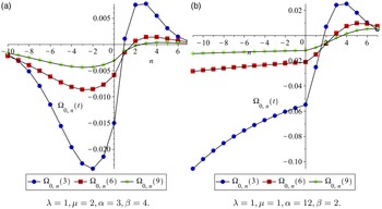Therefore there is no jump at the point 0 and the process is null recurrent. Again, we can get an approximation of the probability current by using (30), the spectral matrix, and the corresponding orthogonal polynomials. In Figure 4 this probability current is plotted as a function of n starting at $j=0$ for $t=3,6,9,$ for a couple of values of the birth–death rates $\lambda,\mu,\lambda_0,\mu_0$ . In both cases we have only one Dirac delta, located at $x=\gamma_+$ .

Figure 4.

The probability current $\Omega_{0,n}(t)$ (30) for the example in Section 4.1 is plotted as a function of n for $t = 3$ (blue circles), $t = 6$ (red squares), and $t =9$ (green diamonds) for a couple of values of the birth–death rates $\lambda,\mu,\lambda_0,\mu_0$ .

4.2. Case 2

Let us now consider a variant of the symmetric bilateral birth–death process with constant rates studied in Example 2.3. The birth–death rates are now given by

\begin{equation*}\lambda_n=\lambda,\quad\mu_n=\mu,\quad \lambda_{-n}=\mu,\quad \mu_{-n}=\lambda, \quad n\in\mathbb{N},\quad \lambda,\mu,\lambda_0,\mu_0>0.\end{equation*}

The matrices $\mathcal{A}^{\pm}$ in (17) and (18) are the same as in the previous case, so that we can use the same notation for the Stieltjes transforms of $\psi^{\pm}$ in (32). Now there is a small change in the formulas (21), but somehow this slightly simplifies the computation of the Stieltjes transforms $B(z;\,\psi_{\alpha\beta})$ , $\alpha,\beta=1,2$ . Again, after rationalizing, we obtain that

\begin{equation*}B(z;\,\psi_{\alpha\beta})=\frac{p_{\alpha\beta}(z)+q_{\alpha\beta}(z)\sqrt{(\lambda+\mu-z)^2-4\lambda\mu}}{D(z)},\quad \alpha,\beta=1,2,\end{equation*}

where

\begin{align*}p_{11}(z)&=(\lambda_0+\mu_0-2\lambda)z+(\lambda -\mu)(\lambda_0 +\mu_0),\quad q_{11}(z)=-(\lambda_0+\mu_0),\\p_{12}(z)&=z^2-(\lambda_0 + \mu_0 + \lambda + \mu)z+(\lambda - \mu)(\lambda_0 + \mu_0),\quad q_{12}(z)=-(\lambda_0+\mu_0-z),\\p_{22}(z)&=\frac{1}{\lambda\mu_0}\left[(\lambda_0 - \lambda)z^3+\big({-}\lambda_0^2 - \lambda_0\mu_0 - 2\lambda_0\mu + 2\mu_0\lambda + \lambda^2 + \lambda\mu\big)z^2\right.\\&\quad \left.+\mu_0\lambda(\lambda - \mu)(\lambda_0 + \mu_0)+(\lambda_0^2\lambda + \lambda_0^2\mu + \lambda_0\mu_0\mu - \lambda_0\lambda^2 + \lambda_0\mu^2 - \mu_0^2\lambda - 2\mu_0\lambda^2)z\right],\\q_{22}(z)&=-\frac{1}{\lambda\mu_0}\left[(\lambda-\lambda_0)z^2+(\lambda_0^2 + \lambda_0\mu_0 - \lambda_0\lambda + \lambda_0\mu - 2\mu_0\lambda)z+\mu_0\lambda(\lambda_0 + \mu_0)\right],\\D(z)&=2z[(\lambda_0 +\mu_0)(\lambda_0 + \mu_0 - \lambda + \mu)-(\lambda_0+\mu_0-\lambda)z].\end{align*}

The spectral matrix $\Psi(x)=\Psi_c(x)+\Psi_d(x)$ now has an absolutely continuous part $\Psi_c(x)$ , given by

(36) \begin{equation}\Psi_c(x)=\frac{\sqrt{(x-\sigma_-)(\sigma_+-x)}}{\pi D(x)}\begin{pmatrix}\lambda_0+\mu_0& \quad \lambda_0+\mu_0-x\\[4pt]\lambda_0+\mu_0-x & \quad q_{22}(x)\end{pmatrix},\quad x\in[\sigma_-,\sigma_+],\end{equation}

where $\sigma_{\pm}=\big(\sqrt{\lambda}\pm\sqrt{\mu}\big)^2$ . For the discrete part $\Psi_d(x)$ we now get easier expressions, since the roots of D(z) are given by 0 and the constant

\begin{equation*}\eta=\frac{(\lambda_0+\mu_0)(\lambda_0+\mu_0-\lambda+\mu)}{\lambda_0+\mu_0-\lambda}.\end{equation*}

After some straightforward computations we have that the discrete part $\Psi_d(x)$ is given by

(37) \begin{align}&\Psi_d(x)=\frac{\mu-\lambda}{\lambda_0+\mu_0+\mu-\lambda}\begin{pmatrix}1 & \quad 1\\[4pt]1&\quad 1\end{pmatrix}\delta_{0}(x)\mathbf{1}_{\{\mu>\lambda\}}\nonumber\\[4pt]&\quad +\frac{(\lambda_0+\mu_0-\lambda)^2-\lambda\mu}{(\lambda_0+\mu_0-\lambda)(\lambda_0+\mu_0+\mu-\lambda)}\begin{pmatrix}1&\quad -\displaystyle\frac{\mu}{\lambda_0+\mu_0-\lambda}\\[12pt]-\displaystyle\frac{\mu}{\lambda_0+\mu_0-\lambda}&\quad \displaystyle\left(\frac{\mu}{\lambda_0+\mu_0-\lambda}\right)^2\end{pmatrix}\delta_{\eta}(x)\mathbf{1}_{\{|\lambda_0+\mu_0-\lambda|>\sqrt{\lambda\mu}\}},\end{align}

where $\mathbf{1}_A$ is the indicator function and $\delta_a(x)$ is the Dirac delta located at $x=a$ . Finally, we can also compute the polynomials generated by the three-term recurrence relation (13). Using the same notation as in (34), we have that $Q_n^1(x)$ and $Q_n^2(x)$ for $n\in\mathbb{N}_0$ are the same as in the previous case in (35), while for $Q_{-n-1}^1(x)$ and $Q_{-n-1}^2(x)$ we only have to change $\lambda$ by $\mu$ in (35). Once more, the transition probability functions $P_{ij}(t)$ can then be approximated using the Karlin–McGregor formula (14). It is possible to see that if $\lambda_0=\lambda$ and $\mu_0=\mu$ we go back to Example 2.3, the example of the symmetric bilateral birth–death process with constant rates.

From (27) and the explicit expression for the spectral matrix, we have that $\int_0^\infty x^{-1}\psi_{11}(x)dx<\infty$ and $\int_0^\infty x^{-1}\psi_{22}(x)dx<\infty$ for $\lambda>\mu$ and any values of $\lambda_0,\mu_0$ . Therefore the process is always transient for $\lambda>\mu$ . If $\lambda\leq\mu$ then both integrals diverge and the process is recurrent. For $\lambda<\mu$ we always have a jump at the point 0, so the process is positive recurrent. If $\lambda=\mu$ then the process is null recurrent. Since the potential coefficients are given here (see (12)) by

\begin{equation*}\pi_0=1,\quad\pi_n=\frac{\lambda_0}{\mu}\!\left(\frac{\lambda}{\mu}\right)^{n-1},\quad\pi_{-n}=\frac{\mu_0}{\mu}\!\left(\frac{\lambda}{\mu}\right)^{n-1},\quad n\in\mathbb{N},\end{equation*}

we have that the invariant distribution $\boldsymbol\pi$ for this process is given by

\begin{equation*}\boldsymbol\pi=\frac{\mu-\lambda}{\mu-\lambda+\mu_0+\lambda_0}\!\left(\cdots,\frac{\mu_0\lambda}{\mu^2},\frac{\mu_0}{\mu},1,\frac{\lambda_0}{\mu},\frac{\lambda_0\lambda}{\mu^2},\frac{\lambda_0\lambda^2}{\mu^3},\cdots\right),\quad \mu>\lambda.\end{equation*}

The graphs of the probability current are similar to the ones plotted in Figure 4 if we choose the same values of the birth–death rates $\lambda,\mu,\lambda_0,\mu_0$ .

Remark 4.2. In Section 5.3 of [Reference Giorno and Nobile13], this example was studied for the particular case of $\lambda_0=\mu_0=\lambda$ . Substituting these values in (36) and (37), we have that the spectral matrix in this particular case is given by $\Psi(x)=\Psi_c(x)+\Psi_d(x)$ , where

\begin{equation*}\Psi_c(x)=\frac{\sqrt{(x-\sigma_-)(\sigma_+-x)}}{\pi x(2\lambda+2\mu-x)}\begin{pmatrix}1&\quad \displaystyle 1-\frac{x}{2\lambda}\\[12pt]\displaystyle 1-\frac{x}{2\lambda}& \quad -1+\displaystyle\left(1-\frac{\mu}{\lambda}\right)\frac{x}{2\lambda}\end{pmatrix},\quad x\in[\sigma_-,\sigma_+],\end{equation*}

with $\sigma_{\pm}=\big(\sqrt{\lambda}\pm\sqrt{\mu}\big)^2$ , and

\begin{equation*}\Psi_d(x)=\frac{\mu-\lambda}{\mu+\lambda}\left[\begin{pmatrix}1 & \quad 1\\[4pt]1&\quad 1\end{pmatrix}\delta_0(x)\mathbf{1}_{\{\mu>\lambda\}}+\begin{pmatrix}1&\quad -\mu/\lambda\\[4pt]-\mu/\lambda&\quad (\mu/\lambda)^2\end{pmatrix}\delta_{2\lambda+2\mu}(x)\mathbf{1}_{\{\lambda>\mu\}}\right].\end{equation*}

An extensive analysis of the probability properties of this example appears in Section 5.3 of [Reference Giorno and Nobile13].