1. Introduction
The sheet flow regime of sediment transport occurs when the fluid flow is sufficiently strong to mobilise a thick and dense layer of particles on the top of a sediment bed. The present paper is focused on uniform, steady and turbulent sheet flows of well-sorted particles in which the low value of the slope allows the neglect of the body force acting on the particles. In such conditions, both granular interactions and turbulent processes are the key mechanisms in momentum and particle diffusion (e.g. Bagnold Reference Bagnold1956; Jenkins & Hanes Reference Jenkins and Hanes1998). The Shields number
 ${\it\theta}$
and the suspension number
 $S$
are the two dimensionless numbers that control sediment transport in this regime (Sumer et al.
Reference Sumer, Kozakiewicz, Fredsøe and Deigaard1996). The Shields number is defined as the ratio between the force exerted by the fluid on a particle at the bed and the apparent weight of a single particle:
 ${\it\theta}={\it\rho}_{f}u_{\ast }^{2}/({\it\rho}_{p}-{\it\rho}_{f})gd_{p}$
where
 ${\it\rho}_{f}$
and
 ${\it\rho}_{p}$
are the density of the fluid and the particles respectively,
 $u_{\ast }$
is the friction velocity,
 $g$
the acceleration due to gravity and
 $d_{p}$
the particle diameter. In the literature, the transition from the bedform regime to the sheet-flow regime occurs at a Shields number around 0.5. Above this value, the bed-load layer thickness and the associated solid load increase with the Shields number (e.g. Einstein Reference Einstein1950; Yalin Reference Yalin1977). The suspension number,
 $S=w_{s}/u_{\ast }$
, characterises the competition between the particle inertia represented by its settling velocity (
 $w_{s}$
) and the magnitude of the turbulent velocity fluctuations represented by the friction velocity (
 $u_{\ast }$
). Following Sumer et al. (Reference Sumer, Kozakiewicz, Fredsøe and Deigaard1996), for
 $S<0.8$
the sheet-flow regime is in the suspension mode in which the suspended load is greater than the bed load. For
 $S>1$
, the sheet-flow regime is in the no-suspension mode in which the bed load dominates over the suspension load.
The challenges in research on the sheet-flow regime reside currently in two complementary aspects. The first one lies in the modelling of the horizontal and vertical momentum transfer mechanisms for both fluid and solid phases. The second one concerns the realisation of controlled sheet-flow experiments providing reliable high-resolution data. At present, only few such datasets exist in the literature and this strongly limits our ability to investigate the validity of sheet-flow models.
The vertical profile of shear stress (i.e. along the flow normal direction) from the free surface down to the non-moving bed can be derived from the horizontal (i.e. streamwise) momentum balance. Under uniform flow conditions, the total shear stress
 ${\it\tau}$
is linear with
 $z$
, the vertical coordinate, and at any given position it balances the weight of the water column above, projected on the streamwise direction
 $x$
. Both the fluid and the granular phase possibly contribute to the total shear stress. In the dilute suspension (usually taken as the flow domain where the volumetric concentration
 ${\it\phi}$
is lower than 0.08, Hsu, Jenkins & Liu Reference Hsu, Jenkins and Liu2004) the total shear stress is balanced by the turbulent Reynolds shear stress which transfers streamwise momentum downward from high-velocity layers to reduced-velocity layers. Within the mobile sediment layer, momentum can be transferred vertically by turbulent fluctuations and/or collisional and frictional interactions between grains. At the bed interface, a plastic threshold imposes a zero velocity shear rate where the friction between grains exactly balances the total shear stress (Coulomb yield criterion, Hanes & Inman Reference Hanes and Inman1985). The vertical profile of particle concentration can be obtained from the vertical momentum balance in which gravity is mainly balanced by two mechanisms: a turbulent dispersion term arising from the effect of turbulent velocity fluctuations on the drag force (e.g. Chauchat & Guillou Reference Chauchat and Guillou2008) and a dispersive force induced by granular interactions (Bagnold Reference Bagnold1954; Wilson Reference Wilson1989; Jenkins & Hanes Reference Jenkins and Hanes1998). This last force originates from collisions and enduring contacts between particles and vanishes at low concentration (
 ${\it\phi}\lesssim 0.08$
) for which particles are fully suspended by the fluid turbulence. Around this limit value of concentration it is likely that a competition between both mechanisms occurs.
Several attempts have been made to model the above mentioned granular interactions in the sheet-flow regime. In his pioneering work, Bagnold (Reference Bagnold1954) proposed a formulation of the granular shear stress proportional to the square of the velocity shear rate and to the square of the particle diameter (inertial regime). He also suggested that the particulate pressure is proportional to the shear stress. More recently, several authors have used the kinetic theory of granular flows to account for the granular contribution to the shear stress (Jenkins & Hanes Reference Jenkins and Hanes1998; Hsu et al.
Reference Hsu, Jenkins and Liu2004; Berzi Reference Berzi2011, amongst others). In this theory, an additional energy equation has to be solved for the granular temperature, which represents the intensity of the particle velocity fluctuations. This variable is used to evaluate the granular shear and normal stresses. During the last decade a phenomenological rheology,
 ${\it\mu}(I)/{\it\phi}(I)$
, has been proposed for dry granular flows (GDR Midi 2004; Forterre & Pouliquen Reference Forterre and Pouliquen2008) in which the inertial number
 $I$
, representing the competition between the timescale of rearrangement to the timescale of deformation of the granular media, controls the shear-to-normal stress ratio
 ${\it\mu}$
and the particle concentration
 ${\it\phi}$
(Andreotti, Forterre & Pouliquen Reference Andreotti, Forterre and Pouliquen2013). This rheology has been used with some success to model laminar bed load (Ouriemi, Aussillous & Guazzelli Reference Ouriemi, Aussillous and Guazzelli2009) and turbulent sheet flow (Revil-Baudard & Chauchat Reference Revil-Baudard and Chauchat2013).
Concerning the turbulent contribution to the total shear stress, it has been observed that the presence of particles can significantly modify the turbulence compared with a clear-water turbulent shear boundary layer (Best et al.
Reference Best, Bennett, Bridge and Leeder1997; Muste et al.
Reference Muste, Yu, Fujita and Ettema2005). In order to account for this effect, several authors have used a mixing length approach with a correction depending on (a) the density stratification rate (e.g. Jenkins & Hanes Reference Jenkins and Hanes1998), (b) the local concentration (Pasini & Jenkins Reference Pasini and Jenkins2005, for example) or (c) the integral of the concentration profile (Revil-Baudard & Chauchat Reference Revil-Baudard and Chauchat2013). Hsu et al. (Reference Hsu, Jenkins and Liu2004) have employed a
 $k$
–
 ${\it\epsilon}$
model with a transfer term related to the particle inertia to account for turbulence modulation induced by the presence of particles. However this turbulence modification remains an open question widely discussed in the research community (Castro-Orgaz et al.
Reference Castro-Orgaz, Giráldez, Mateos and Dey2012). The concentration profile in the dilute region of the flow is usually modelled by the so-called Rouse profile. It is based on a balance between the downward settling flux and the upward turbulent dispersion flux. This last term is classically modelled by a Fickian diffusion law as the product of the sediment diffusivity times the local vertical gradient of concentration (Graf & Cellino Reference Graf and Cellino2002). The sediment diffusivity is related to the turbulent eddy viscosity divided by the Schmidt number (
 ${\it\sigma}_{s}$
) which is usually tuned to fit experimental measurements.
Laboratory experiments for the study of the vertical structure of turbulent two-dimensional mean sheet flows are very rare so far. The main reasons for this are the difficulties of measuring both the velocity and the sediment concentration in the same sample volume under such extreme concentration conditions and with a spatio-temporal resolution sufficiently high to resolve turbulent eddies down to the particle scale. Furthermore, the importance of the Reynolds shear stress in the momentum balance across the active sheet-flow layer imposes the performing of quasi-instantaneous two-component (2C) velocity measurements. Few flow measurement systems are adapted to such challenging flow conditions. Experiments were mainly conducted in pipe flows by Daniel (Reference Daniel1965), Wilson (Reference Wilson1966), Nnadi & Wilson (Reference Nnadi and Wilson1992) and Pugh & Wilson (Reference Pugh and Wilson1999). These studies examined the time-averaged volumetric concentration and streamwise velocity (
 $u$
) using a point-wise gamma-ray technique and a point-wise conductivity probe, respectively. Sumer et al. (Reference Sumer, Kozakiewicz, Fredsøe and Deigaard1996) carried out sheet-flow experiments in an open-channel flume (with and without a rigid lid at the top) using point-wise capacity probes for the concentration measurements and a Pitot tube for the local streamwise velocity measurements. More recently, Cowen et al. (Reference Cowen, Dudley, Liao, Variano and Liu2010) have developed a Boroscopic technique to measure the streamwise velocity profile inside the dense moving bed layer. However, only a single velocity profile corresponding to one flow configuration has been published so far.
All these experiments used intrusive point-wise techniques subjected to local flow perturbations and providing only non-collocated one-component (1C) velocity and concentration time series. Consequently, the analysis of these data was restricted to the interpretation of mean profiles of independently measured quantities with no direct quantification of the co-variances such as the Reynolds shear stress or the turbulent sediment fluxes. More recently, Armanini et al. (Reference Armanini, Capart, Fraccarollo and Larcher2005), Capart & Fraccarollo (Reference Capart and Fraccarollo2011) and Spinewine et al. (Reference Spinewine, Capart, Fraccarollo and Larcher2011) have developed a video technique to get instantaneous 2C particle velocity and mean concentration profiles in the near-wall region. To the best of our knowledge, this dataset is currently the only one which provides both particle velocity and concentration profiles under sheet-flow conditions in an open channel flow. The fact that velocity and concentration measurements are neither collocated nor synchronised and that they were measured at the sidewall constitute the main restrictions of this dataset.
In the present paper, a new sheet-flow experiment carried out in an open channel is presented. A multi-frequency acoustic concentration velocity profiler (ACVP, Hurther et al. Reference Hurther, Thorne, Bricault, Lemmin and Barnoud2011; Naqshband et al. Reference Naqshband, Ribberink, Hurther and Hulscher2014) is used to provide non-intrusive vertical profiles across the suspension and the sheet-flow layers of collocated 2C velocities and particle concentration. The mean profiles are analysed to discuss the physical mechanisms responsible for the momentum and concentration fluxes across the entire water column and to assess different available modelling approaches. The paper is organised as follows: in § 2, the experimental setup and the data processing of the acoustic measurements are described. In § 3, the mean profiles of streamwise velocity, concentration, turbulent shear stress and sediment flux are presented. The vertical structure of the flow is outlined from momentum and concentration diffusivity profiles and further analysed based on mixing length, Stokes and inertial numbers. Then, the measurements are compared with different constitutive laws to discuss the modelling perspectives of this new dataset. In § 4 the obtained results are discussed and in § 5, the main conclusions of this paper are summarised.
2. Experimental setup and flow conditions
In this section, we first present the experimental setup composed of the tilting flume and the measurement equipment. Secondly, the experimental protocol and methodology are described. Finally, the data processing method and the corresponding mean flow data are analysed to verify (a) the establishment of two-dimensional mean flow conditions as a steady uniform sheet flow and (b) the validity of the sediment transport measurements provided by the ACVP.
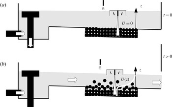
Sketch of the experimental setup in its initial (a) and running (b) states.

2.1. Experimental facility
The LEGI/ENSE3 tilting flume is
 $L=10~\text{m}$
long and
 $W=0.35~\text{m}$
wide with a bed slope set to a value of
 $S_{0}=0.005$
. A 3 m long by 11 cm high sediment reservoir is installed in the channel bed 2 m before the channel outlet (see figure 1). Elsewhere the flume bed is covered by glued particles to enhance the bed roughness and facilitate the full development of the boundary layer before the test section. The sediments are irregularly shaped (PMMA, density
 ${\it\rho}_{p}=1192~\text{kg}~\text{m}^{-3}$
) with a tangent of the angle of repose measured at
 ${\it\mu}_{s}=0.7$
in dry conditions. The particle size distribution is well-sorted and the particle diameters are in the range
 $d_{p}\in 2.5{-}3.5~\text{mm}$
(table 1). The mean settling velocity is equal to
 $w_{s}=5.59\pm 1.1~\text{cm}~\text{s}^{-1}$
which was determined experimentally from settling tests in a still water tank. The flume is equipped with an acoustic limnimeter mounted on a moveable trolley for the measurement of the water level time series at a rate of 200 Hz in the test section. These water level measurements are synchronised with the data acquisitions of the ACVP.
Sediment and flow properties.

The ACVP is a 1D2C system measuring the co-located streamwise and vertical velocity components as well as the particle volumetric concentration over a vertical profile of 25 cm extending from the bed interface to the top of the free surface. The originality of this acoustic flow instrumentation lies in the combination of the multi-bistatic ADVP technology (acoustic Doppler velocity profiler, Hurther & Lemmin Reference Hurther and Lemmin2001, Reference Hurther and Lemmin2008; Mignot, Hurther & Barthelemy Reference Mignot, Hurther and Barthelemy2009) with the multi-frequency ABS technology (acoustic backscattering system, Thorne & Hanes Reference Thorne and Hanes2002; Thorne, Hurther & Moate Reference Thorne, Hurther and Moate2011; Thorne & Hurther Reference Thorne and Hurther2014) into a single ACVP system as proposed by Hurther et al. (Reference Hurther, Thorne, Bricault, Lemmin and Barnoud2011).
Recently, the profiling of velocity and sediment transport quantities across both the suspension and the bed layers has provided new insights into a variety of sediment transport processes (Hurther & Thorne Reference Hurther and Thorne2011; Chassagneux & Hurther Reference Chassagneux and Hurther2014; Naqshband et al.
Reference Naqshband, Ribberink, Hurther and Hulscher2014). The same methodology and data validation technique is applied herein as discussed below. The spatio-temporal resolution of the measurements is equal to
 ${\rm\Delta}z=3~\text{mm}$
along the vertical direction and
 $1/78~\text{s}$
, respectively. The time rate of the concentration measurement is set to 4.9 Hz to guarantee a statistical bias lower than 15 % as discussed in Thorne & Hurther (Reference Thorne and Hurther2014). The acoustic bed interface tracking (ABIT) method proposed by Hurther & Thorne (Reference Hurther and Thorne2011) is used here for the localisation of the bed interface at a time rate of 7.8 Hz. This bed localisation technique allows the reduction of Doppler noise effects in the mean velocity and sediment transport profiles by forcing the instantaneous Doppler velocities to zero below the detected bed level position. Flow intrusiveness of the ACVP sensors is minimised by placing the system into a vacuum box. The lower end of this box is slightly below the free-surface level as illustrated in figure 1. Despite the fact that the box generates a roughly 1 cm thick mixing layer in the upper part of the water column, the vacuum box guarantees a negligible impact of the instrument on the sediment bed. Moreover, it provides velocity measurements over the entire shear boundary layer height as shown below.
2.2. Experimental protocol and flow properties
The particles transported during the experiment are not recirculated. This induces bed erosion during the runs which requires particular attention to fulfilling steady uniform flow conditions as discussed below. In order to minimise the transient period associated with the setup of the targeted flow discharge, the flume is first filled slowly with no sediment movement on the horizontally levelled particle bed until the still water level has reached a value just above the final normal flow depth. At this stage, the sluice gate at the flume exit is still closed and a circular shaped weir located in the upstream reservoir evacuates the entire water discharge as illustrated in figure 1(a). The sluice gate is suddenly opened, causing a rapid water level drop to inactivate the circular weir and to transfer the entire flow discharge of
 $Q_{f}=31~\text{l}~\text{s}^{-1}$
into the tilting flume. After less than 30 s the water flow and the sheet-flow layer are fully developed with a normal flow depth of
 $H_{f}=0.17~\text{m}$
above the bed interface and a mean bulk flow velocity of
 $U=0.52~\text{m}~\text{s}^{-1}$
. This experimental procedure is repeated for
 $N=11$
runs in order to increase the statistical convergence of the averaged flow quantities, as shown in the next section.
The bulk Reynolds number
 $\mathit{Re}=UH_{f}/{\it\nu}_{f}$
is of the order of
 $10^{5}$
. The Reynolds roughness number
 $\mathit{Re}_{\ast }=u_{\ast }^{\prime }k_{s}/{\it\nu}_{f}$
can roughly be estimated from the friction velocity as
 $u_{\ast }^{\prime }=\sqrt{gH_{f}S_{0}}=0.09~\text{m}~\text{s}^{-1}$
and the bed roughness as
 $k_{s}=2.5d_{p}$
. This gives
 $\mathit{Re}_{\ast }=375$
. The values of the two Reynolds numbers indicate that the flow is fully turbulent and fully hydraulically rough. The flow is subcritical with a Froude number
 $\mathit{Fr}=U/\sqrt{gH_{f}}\approx 0.4$
where
 $g$
is the gravitational acceleration.
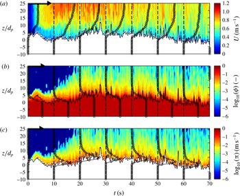
Figure 2 presents an example of the measured profiles of the streamwise velocity (a), the volumetric particle concentration (b) and the streamwise sediment flux
 ${\it\pi}={\it\phi}u$
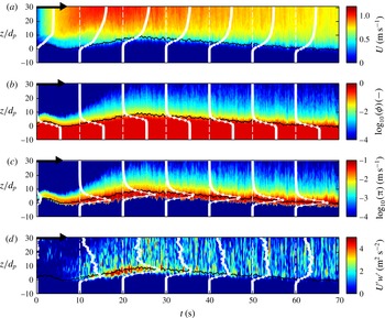
(c) for one of the 11 runs. The black solid line represents the detected bed interface. The vertical axis is the vertical coordinate made dimensionless by the particle diameter. Due to the highly turbulent flow conditions, these data have been low-pass filtered using a moving rectangular window at a cutoff frequency of 4.9 Hz. The black solid lines with circle markers represent the vertical profiles averaged over 6 s and shown every 10 s. As can be seen from these figures, the run can be divided into a transient phase of approximately 30 s followed by a quasi-steady bed erosion phase of roughly 40 s long. During the transient phase, the bed is first abruptly eroded over the first 5 s and more slowly accreted until
 $t=28~\text{s}$
. The corresponding streamwise velocity field shows a severe acceleration phase reaching velocities of approximately
 $1~\text{m}~\text{s}^{-1}$
associated with the bed erosion phase and a bulk flow deceleration period during the accretion phase. This transient phase also shows a strong vertical heterogeneity in the velocity profiles since a low-velocity near-bed region appears to persist over the first 20 s (seen as a blue coloured near-bed domain in figure 2
a). This vertical flow heterogeneity disappears after 30 s with the establishment of typical shear flow profiles of negligibly low velocity at the bed interface position.
Colourplot of the filtered instantaneous streamwise velocity (a), concentration (b) and two-dimensional sediment flux (c). The filtered detected bed-interface positions are presented by the solid black lines. The vertical axis is made dimensionless by the particle diameter. The curves show the vertical profiles averaged over 6 s and represented every 10 s. The arrow at the top left corner of each panel corresponds to
 $u=1~\text{m}~\text{s}^{-1}$
,
 ${\it\phi}=0.55$
and
 ${\it\pi}=0.05~\text{m}~\text{s}^{-1}$
respectively.

The volumetric concentration time series (in
 $\log _{10}$
) show the development of a suspension layer over the first 25 s from an initial value
 ${\it\phi}\approx 0$
to values in the
 ${\it\phi}\approx 0.001$
range. In the near-bed region the concentration reaches a maximum value
 ${\it\phi}^{m}=0.55$
below the bed interface position. In particular, the maximum bed concentration value follows quite perfectly the time evolution of the bed level position over the entire run. This unforced behaviour strongly supports the validity of the acoustic concentration measurements in the dense near-bed flow region.
The colourplots of the sediment flux in figure 2(c) reveal high near-bed sediment flux values over the entire run. The suspension flux over the transient phase is negligibly low. This can be attributed to the negligibly low suspension concentration values since the bulk flow velocity is significantly high during this phase. In the quasi-steady erosion phase, the sediment flux profiles show fairly steady shapes of the profiles relative to the bed interface position.
Although not shown here, the 11 runs have a very similar spatio-temporal structure at large flow scales and with a randomly distributed short scale variability over the different runs. The repeated run behaviour allows us to apply the ensemble averaging technique described in the following section. Another interesting point in figure 2 is the range of bed level variability at short timescales. It is found to reach several particle diameters. The origin of this phenomenon is addressed in the discussion section of this paper. From the present analysis of the time series it can be deduced that time averaging over the complete duration of a run is not well adapted to satisfy steady uniform conditions. Therefore, a specific averaging technique has been applied as described in § 2.4.
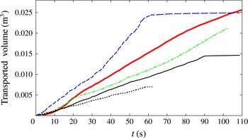
Time evolution of the volume of transported sediment (acoustic estimation) for different flow regimes, from low bed load (⋯) to an intense sheet flow (- - -). The thick line corresponds to the ensemble-averaged sheet flow experiment considered in this paper.

Comparison between the volume of transported sediment evaluated acoustically
 $(\mathscr{V}_{ACVP})$
and by weighing (
 $\mathscr{V}_{w}$
).

2.3. Validation of acoustic sediment transport measurements
In order to test quantitatively the validity of the acoustic sediment flux measurements, the volume of transported particles estimated acoustically has been directly compared to the volume of particles collected in two sediment traps located downstream of the test section. The acoustic estimation of the total volume of transported sediment,
 $\mathscr{V}_{ACVP}(t=t_{max})$
, is calculated from:
 $$\begin{eqnarray}\mathscr{V}_{ACVP}(t)=W\int _{0}^{t}\int _{-\infty }^{+\infty }u(t,z){\it\phi}(t,z)\text{d}z\text{d}t,\end{eqnarray}$$
where
 $W$
represents the flume width. The mass balance technique consists of weighing the dried amount of particles
 $\mathscr{V}_{w}$
collected after a run. The obtained mass is divided by the particle density for comparison with the acoustic estimation
 $\mathscr{V}_{ACVP}(t_{max})$
.
Figure 3 represents the time evolution of the transported particle volume,
 $\mathscr{V}_{ACVP}(t_{max})$
. In order to carefully validate the acoustic measurement, the comparison has been done for four significantly different flow conditions (see table 2). The dotted line corresponds to a relatively low-bed-load regime while the dashed one corresponds to an intense sheet flow. The discrepancy between the two estimations is found to be less than 18 %. The discrepancies for the lowest bed load and the most intense sheet flow are 5 % and 10 % respectively. Since the transported volume estimated acoustically is obtained by adding up a very large number of sediment flux realisations, the low relative errors obtained support the presence of negligibly low systematic errors in the sediment flux measurements.
Another interesting aspect is seen in the trend of the thickest curve in figure 3 which corresponds to an ensemble average of
 $\mathscr{V}_{ACVP}(t)$
over the 11 repeated runs. It shows a clear slope break from a high to a lower value of the sediment transport rate around
 $t=30~\text{s}$
. This change of sediment transport rate is in very good agreement with the observations made in figure 2 on the presence of a transient phase followed by a fairly quasi-steady erosion phase. The results shown here strongly support the validity of the sediment transport measurement provided by the ACVP.
2.4. Experiment repeatability, flow steadiness and uniformity
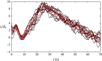
In order to ensemble average the measured quantities over the 11 runs, the repeatability of the experiments is analysed herein. A representative criterion is the ensemble standard deviation associated with the 11 realisations. Figure 4 shows the time series of the bed level position for the 11 realisations of the experiment. Each realisation has been time referenced to an initial event of a free-surface water drop occurring after the gate opening. The drop is set to 5 % as
 $H_{f}(t=0)=0.95H_{max}$
, where
 $H_{max}$
is the initial water level in figure 1(a). In figure 4 the ensemble average of the bed level position is plotted (thick grey line, red online) and bounded by plus and minus the ensemble standard deviation (grey dot-dashed lines, red online). It is shown that the value of the ensemble standard deviation is around one particle diameter and it is of the order of the variability in a single time series. This indicates the very high degree of repeatability of the experiment in terms of bed morphology evolution.
Time evolution of the bed interface positions filtered at 0.333 Hz and made dimensionless by the particle diameter for the 11 realisations (- - -). Ensemble average (thick grey line, red online) boxed by plus and minus the associated standard deviation (grey dot-dashed line, red online).

Since the bed is eroded during the experiment, the interval over which the flow can be time-averaged has to be determined. The ensemble average of the bed level time series (figure 4) permits the evaluation of the mean erosion rate in the quasi-steady phase (
 $t>30~\text{s}$
) to a value of one particle diameter every 6 s. This time interval (
 ${\rm\Delta}t=6~\text{s}$
) is sufficiently short to assume a constant bed level and long enough to be statistically representative of the largest turbulent flow scales since
 ${\rm\Delta}t\approx 30T_{LSS}$
where
 $T_{LSS}\approx 0.7H_{f}/U$
represents a characteristic scale of the time spent by the biggest turbulent structure in the measurement volume (Muste, Yu & Spasojevic Reference Muste, Yu and Spasojevic2004).
Colourplot of the ensemble-averaged and filtered instantaneous streamwise velocity (a), concentration (b), two-dimensional sediment flux (c) and absolute Reynolds stress (d). The ensemble-averaged and filtered detected bed-interface positions are presented by the solid black lines. The vertical axis is made dimensionless by the particle diameter. The curves show the ensemble-averaged vertical profiles averaged over 6 s and represented every 10 s. The arrow at the top left corner of each panel corresponds to
 $u=1~\text{m}~\text{s}^{-1}$
,
 ${\it\phi}=0.55$
,
 ${\it\pi}=0.05~\text{m}~\text{s}^{-1}$
and
 $\langle u^{\prime }w^{\prime }\rangle =0.003~\text{m}^{2}~\text{s}^{-2}$
respectively.

The selection of the appropriate 6 s time interval in the quasi-steady bed erosion phase of the individual runs (i.e. for
 $t>30~\text{s}$
) is based on the consideration of the ensemble-averaged data shown in figure 5. In addition to the steady flow conditions, the selected 6 s time interval must also satisfy uniform flow conditions in contrast to accelerated or decelerated flow regimes. The velocity, concentration and sediment flux time series in figure 5 show that the most steady time interval is seen between
 $t=40~\text{s}$
and
 $t=50~\text{s}$
. In this time interval, both the magnitudes of the measured quantities at a given distance from the bed and the shape of the vertical profiles are very similar. The mean absolute Reynolds shear stress is shown in figure 5(d). In terms of flow uniformity, it can clearly be observed that the vertical profiles exhibit the most linear trend versus
 $z$
at the time
 $t=40~\text{s}$
. Before and after this time, the vertical profiles follow, respectively, a concave and a convex shape. Song & Graf (Reference Song and Graf1994) and Yang & Chow (Reference Yang and Chow2008) showed that the deviation from a linear shear stress profile is an accurate indication of the flow non-uniformity. This is further confirmed here since the concave shear stress profile is associated with an accelerated bulk flow whereas the convex shape is obtained during the decelerating phase for
 $t\gtrsim 50~\text{s}$
. As a consequence, the 6 s time interval over which the flow steadiness will be tested quantitatively is taken as
 $[40{-}46~\text{s}]$
in figure 5.
The analysis of the statistical properties of the ensemble-averaged velocity, concentration and streamwise sediment flux profiles
 $\langle u\rangle (z)$
,
 $\langle w\rangle (z)$
,
 ${\it\phi}(z)$
and
 ${\it\pi}(z)$
relies on the calculation of the statistical moments between
 $t_{1}=40~\text{s}$
and
 $t_{2}=46~\text{s}$
as:
 $$\begin{eqnarray}\displaystyle & & \displaystyle \langle u\rangle (z)=\frac{1}{N}\mathop{\sum }_{i=1}^{N}\left(\frac{1}{{\rm\Delta}t}\int _{t_{1}}^{t_{2}}u_{i}(t,z)\text{d}t\right),\end{eqnarray}$$
 $$\begin{eqnarray}\displaystyle & & \displaystyle \langle w\rangle (z)=\frac{1}{N}\mathop{\sum }_{i=1}^{N}\left(\frac{1}{{\rm\Delta}t}\int _{t_{1}}^{t_{2}}w_{i}(t,z)\text{d}t\right),\end{eqnarray}$$
 $$\begin{eqnarray}\displaystyle & & \displaystyle {\it\phi}(z)=\frac{1}{N}\mathop{\sum }_{i=1}^{N}\left(\frac{1}{{\rm\Delta}t}\int _{t_{1}}^{t_{2}}{\it\phi}_{i}(t,z)\text{d}t\right),\end{eqnarray}$$
 $$\begin{eqnarray}\displaystyle & & \displaystyle {\it\pi}(z)=\frac{1}{N}\mathop{\sum }_{i=1}^{N}\left(\frac{1}{{\rm\Delta}t}\int _{t_{1}}^{t_{2}}u_{i}(z,t){\it\phi}_{i}(z,t)\text{d}t\right),\end{eqnarray}$$
 $i$
standing for the realisation number. Under the assumption of ergodicity, the equivalent period of time averaging for a steady flow is
 $N\times {\rm\Delta}t=66~\text{s}$
. Over this averaging interval, the first-order moments have a bias error in the range of 1 %. The Reynolds components of the velocity are estimated as:
 $$\begin{eqnarray}\displaystyle & & \displaystyle u_{i}^{\prime }(t,z)=u_{i}(t,z)-\langle u\rangle (z),\end{eqnarray}$$
 $$\begin{eqnarray}\displaystyle & & \displaystyle w_{i}^{\prime }(t,z)=w_{i}(t,z)-\langle w\rangle (z).\end{eqnarray}$$
The mean Reynolds shear stress
 ${\it\rho}_{f}\langle u^{\prime }w^{\prime }\rangle (z)$
is calculated as:
 $$\begin{eqnarray}{\it\rho}_{f}\langle u^{\prime }w^{\prime }\rangle (z)={\it\rho}_{f}\frac{1}{N}\mathop{\sum }_{i=1}^{N}\left(\frac{1}{{\rm\Delta}t}\int _{t_{1}}^{t_{2}}u_{i}^{\prime }(t,z)w_{i}^{\prime }(t,z)\text{d}t\right).\end{eqnarray}$$
In order to check the flow steadiness over the time interval
 $[40{-}46~\text{s}]$
, the ensemble-averaged streamwise velocity profile given by (2.2) is calculated over the time interval
 $[40{-}43~\text{s}]$
and compared to the one obtained over the time interval
 $[43{-}46~\text{s}]$
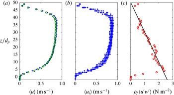
. As shown in figure 6(a), the similarity of the two profiles further confirms the steadiness of the flow over the time interval
 $[40{-}46~\text{s}]$
. A mixing layer induced by the vacuum box is observed on this plot (
 $z/d_{p}>40$
), but it represents only 20 % of the total water depth. In figure 6(b) the profile of streamwise velocity averaged over the time interval
 $[40{-}46~\text{s}]$
for each of the 11 realisations is shown. The very good agreement between the different profiles in terms of magnitude and shape along
 $z$
further supports the high degree of experiment repeatability. Finally, the quantitative validation of the flow uniformity condition is based on the representation in figure 6(c) of the ensemble-averaged absolute Reynolds shear stress profile given by (2.8). As previously observed in figure 5, this profile exhibits a linear evolution versus
 $z$
over the bulk flow region, which is a clear indication of an established uniform flow (Yang & Chow Reference Yang and Chow2008). The linear fit of the shear stress profile (solid black line in figure 6
c) crosses the zero axis at the vertical coordinate
 $z/d_{p}=50$
. This position corresponds to a physical distance of 17 cm above the bed interface which is in very good agreement with the value of the measured flow depth. This aspect further indicates the full development of the shear boundary layer over the entire flow depth. In this section, the high degree of repeatability, steadiness and uniformity of the present experiment over the selected averaging interval of
 $[40{-}46~\text{s}]$
has been demonstrated. These data are used in the following to investigate the vertical structure of the uniform steady sheet flow.
(a) Mean streamwise velocity profiles averaged over
 $t\in [40{-}43]~\text{s}$
(
 $+$
) and over
 $t\in [43{-}46]~\text{s}$
(○). (b) Mean streamwise velocity profiles averaged over
 $t\in [40{-}46]~\text{s}$
for the 11 realisations. (c) Absolute Reynolds shear stress
 ${\it\rho}_{f}\langle u^{\prime }w^{\prime }\rangle$
(○) and linear fit (——).

Concerning the acoustic measurement uncertainties, Hurther & Lemmin (Reference Hurther and Lemmin2001, Reference Hurther and Lemmin2008) showed that the relative uncertainty in the mean velocity provided by a pulse-coherent ADVP technology (similar to the ACVP technology applied herein) is of the order of 1 % due to the misalignment errors of the sensors in the submillimetre range. The near-bed velocity measurement is dependent on the bed interface detection, therefore the measurement uncertainty close to the bed cannot be trivially evaluated. Nevertheless, the obtained accuracy of the measured transported volume for different flow conditions (see table 2) suggests negligibly low systematic errors in the velocity and concentration measurements. Considering the statistical bias error of 15 % for the instantaneous concentration measurement, the relative uncertainty in the mean concentration data reduces to 1 % (Thorne & Hurther Reference Thorne and Hurther2014). The use of a central derivative scheme leads to relative uncertainties in the velocity gradients below 16 % for
 $z/d_{p}<10$
and which reach 40 % for
 $z/d_{p}=14$
. Above this position the relative uncertainty diverges to infinity since the velocity gradients vanished. Concerning the concentration gradient, the relative uncertainty is below 5 % for
 $z/d_{p}<14$
.
3. Results
In this section, we present and discuss the vertical profiles of velocity, concentration, sediment flux and turbulent shear stress measured with the methodology described in the previous section. Moreover, the profiles of momentum and concentration diffusivities are presented and the vertical structure of the flow is analysed in terms of mixing length, Stokes and inertial numbers. Finally, the measurements are compared to different modelling approaches found in the literature.
3.1. Mean profiles
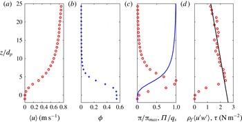
Figure 7 shows the vertical profiles of streamwise velocity (a), volumetric concentration (b), sediment flux repartition (c) and absolute Reynolds shear stress (d). For all plots, the vertical axis
 $z$
is made dimensionless by the particle diameter and its origin is taken at the vertical position where the mean streamwise velocity is lower than 1 % of the bulk flow velocity
 $U$
. This position is denoted as the bed interface in the following.
(a) Mean streamwise velocity profile. (b) Mean concentration profile. (c) Sediment flux (○) and cumulative sediment flux (——) per unit width, normalised by their maximum value. (d) Absolute Reynolds shear stress (○) and total shear stress (——).

Just above the bed interface the velocity profile shown in figure 7(a) increases exponentially with the vertical distance to the bed. Above this exponential layer the velocity profile exhibits a linear behaviour including an inflection point. In the region
 $5\lesssim z/d_{p}\lesssim 14$
, the vertical profile follows a logarithmic shape.
The concentration profile presented in figure 7(b) shows that concentration decreases linearly for
 $2\lesssim z/d_{p}\lesssim 4{-}5$
whereas for
 $z/d_{p}\gtrsim 4{-}5$
the concentration decreases exponentially with
 $z$
. This behaviour will be discussed in the following subsection.
In order to study the solid load repartition along the vertical direction, the cumulative profile of volumetric sediment flux is evaluated over the interval
 $[40{-}46~\text{s}]$
as
 $$\begin{eqnarray}{\it\Pi}(z)=\int _{-\infty }^{z}{\it\pi}(z)\text{d}z.\end{eqnarray}$$
Figure 7(c) presents both the vertical distribution of the sediment flux
 ${\it\pi}(z)$
and the cumulative flux
 ${\it\Pi}(z)$
, normalised by their maximum values. A peak of sediment flux is seen at the position
 $z/d_{p}\approx 4$
. The representation of the cumulative sediment flux shows that roughly half of the total solid load is transported below the position
 $z/d_{p}\approx 4{-}5$
, where the concentration profile is linear and the other half is transported in the layer lying above over which the concentration profile decreases exponentially.
As mentioned previously, the linearity of the turbulent Reynolds stress with
 $z$
indicates the high degree of flow uniformity (figure 7
d). Under uniform flow conditions, the streamwise momentum budget for the fluid–particle mixture is (Revil-Baudard & Chauchat Reference Revil-Baudard and Chauchat2013):
 $$\begin{eqnarray}0={\displaystyle \frac{\text{d}R_{xz}^{f}}{\text{d}z}}+{\displaystyle \frac{\text{d}{\it\tau}_{xz}^{p}}{\text{d}z}}+{\it\rho}_{m}gS_{f},\end{eqnarray}$$
where
 $S_{f}$
is the friction slope,
 ${\it\tau}_{xz}^{p}$
is the intergranular shear stress,
 $R_{xz}^{f}$
is the turbulent Reynolds shear stress and
 ${\it\rho}_{m}=(1-{\it\phi}){\it\rho}_{f}+{\it\phi}{\it\rho}_{p}$
is the mixture density. The viscous contribution can be neglected as shown by Revil-Baudard & Chauchat (Reference Revil-Baudard and Chauchat2013). By integrating equation (3.2) between a given position
 $z$
and the free surface
 $z=H_{f}$
the momentum balance can be written as:
 $$\begin{eqnarray}R_{xz}^{f}(z)+{\it\tau}_{xz}^{p}(z)={\it\tau}(z)={\it\rho}_{m}gS_{f}(H_{f}-z).\end{eqnarray}$$
Assuming that the granular contribution is negligible in the upper part of the flow (
 $z/d_{p}\gtrsim 5$
), the single contribution to the total shear stress is the turbulent one. Therefore, the linear fit of the measured turbulent shear stress in the upper part of the flow can be used to evaluate the total shear stress profile
 ${\it\tau}(z)$
over the entire water column, from the free surface down to the bed interface. The value of the total shear stress at the bed interface provides the friction velocity as:
 ${\it\tau}(z=0)={\it\rho}_{f}u_{\ast }^{2}$
. This method gives a value of
 $u_{\ast }=5.0~\text{cm}~\text{s}^{-1}$
corresponding to a Shields number value of
 ${\it\theta}=0.44$
. This indicates a sediment transport regime at the transition between the bed-load and the sheet-flow regime. The corresponding suspension number value is
 $S=w_{s}/u_{\ast }=1.1$
indicating a transport regime at the transition between the suspension and the no-suspension mode (Sumer et al.
Reference Sumer, Kozakiewicz, Fredsøe and Deigaard1996).
Another classical method to evaluate the friction velocity is the momentum balance for the water column. This leads to the well-known energy slope formulation as
 $u_{\ast }^{m}=(gr_{b}S_{0})^{1/2}=6.2~\text{cm}~\text{s}^{-1}$
, where the equivalent hydraulic radius
 $r_{b}$
is evaluated with the method proposed by Vanoni & Brooks (Reference Vanoni and Brooks1957) for the sidewall corrections. With this estimate of the friction velocity, the Shields number becomes
 ${\it\theta}^{m}=0.68$
. It must be recalled that the classical log-fit method for the evaluation of the friction velocity is not adapted to the sheet-flow conditions investigated herein. The application of this method to mobile bed flow conditions is ambiguous since the origin of the vertical axis is chosen arbitrarily and the von Karman constant is subject to variations around the value of 0.41 due to the presence of moving particles (Vanoni Reference Vanoni1975). This point will be discussed in detail in the following. Regarding the difference of approximately 20 % between the two different friction velocity estimations, Hurther, Lemmin & Terray (Reference Hurther, Lemmin and Terray2007) obtained similar differences under uniform and fixed rough bed flow conditions. Moreover, van der A et al. (Reference van der A, O’Donoghue, Davies and Ribberink2011) demonstrated the validity of the Reynolds bed shear stress method by comparing it to the classical log-fit method. Very good agreement was found in their turbulent rough bed oscillatory flow for the low roughness case (fixed sand particles).
The total solid load per unit width is computed from (3.1) as
 $q_{s}={\it\Pi}(Hf)=7.1\times 10^{-3}~\text{m}^{2}~\text{s}^{-1}$
and in dimensionless form as:
 $$\begin{eqnarray}{\it\psi}=q_{s}\Big/\sqrt{({\it\rho}_{p}-{\it\rho}_{f})gd_{p}^{3}/{\it\rho}_{f}}=3.2.\end{eqnarray}$$
This value can be compared with the result of Meyer-Peter & Muller (Reference Meyer-Peter and Muller1948)’s formula
 ${\it\psi}=8({\it\theta}-{\it\theta}_{c})^{3/2}$
, where
 ${\it\theta}_{c}=0.05$
is the critical threshold value for the initiation of particle motion. Using
 ${\it\theta}=0.44$
, the resulting dimensionless solid load is
 ${\it\psi}=1.9$
which is 40 % lower than the measured value. This value lies within the range of variation seen in Meyer-Peter & Muller (Reference Meyer-Peter and Muller1948)’s measurements. These experimental data were subject to large measurement uncertainties for the solid load and the bed shear stress estimates and therefore we consider this comparison as good. Moreover, if the larger Shields number of
 ${\it\theta}^{m}=0.68$
is used, the dimensionless solid load becomes
 ${\it\psi}=5$
which again lies within the range of uncertainties seen in the data of Meyer-Peter & Muller (Reference Meyer-Peter and Muller1948). This further confirms the validity of the coupled sediment transport and flow forcing measurements provided by the ACVP technology.
3.2. Vertical structure of the flow
When sediment particles are transported in a turbulent boundary layer, streamwise momentum is diffused downward from the bulk flow toward the fixed sediment bed while sediment concentration is diffused upward from the dense moving bed toward the dilute suspension. The nature of these mixing processes depends on the local properties of the flow and a quantitative understanding of these mechanisms is the key issue for an accurate modelling of sediment transport.
Assuming that the shear stress follows a Fickian law, i.e the momentum flux is proportional to its spatial derivative, one can write the following relationship for the total shear stress:
 $$\begin{eqnarray}{\it\tau}={\it\rho}_{m}{\it\epsilon}_{m}\left|\frac{\text{d}u}{\text{d}z}\right|,\end{eqnarray}$$
where
 ${\it\epsilon}_{m}$
represents the momentum diffusivity which has the dimension of a kinematic viscosity. As explained above, the vertical profile of total shear stress
 ${\it\tau}(z)$
is obtained by a linear fit of the turbulent Reynolds shear stress measurements in the dilute region (see figure 7). The vertical profile of mean velocity shear rate
 $(\text{d}u/\text{d}z)$
is calculated from the mean velocity profile. Consequently, the vertical profile of momentum diffusivity
 ${\it\epsilon}_{m}(z)$
can be evaluated as:
 $$\begin{eqnarray}{\it\epsilon}_{m}=\frac{{\it\tau}}{{\it\rho}_{m}\left|\displaystyle \frac{\text{d}u}{\text{d}z}\right|},\end{eqnarray}$$
where the spatial derivative in
 $z$
is approximated by a central derivative scheme.
Following the idea originally introduced by Rouse (Reference Rouse1937), the sediment volume balance in the vertical direction can be written as an equilibrium between the downward settling flux
 $w_{s}{\it\phi}$
and an upward turbulent dispersion or resuspension flux
 ${\it\epsilon}_{p}(\text{d}{\it\phi}/\text{d}z)$
. Using a similar Fickian approach for the particle flux, the following equation is obtained:
 $$\begin{eqnarray}w_{s}{\it\phi}-{\it\epsilon}_{p}\displaystyle \frac{\text{d}{\it\phi}}{\text{d}z}=0.\end{eqnarray}$$
The concentration diffusivity
 ${\it\epsilon}_{p}$
can be evaluated from the mean concentration profile as:
 $$\begin{eqnarray}{\it\epsilon}_{p}=\frac{w_{s}{\it\phi}}{\displaystyle \frac{\text{d}{\it\phi}}{\text{d}z}},\end{eqnarray}$$
where the vertical gradient of concentration is also computed using a finite difference central scheme.
Following the concept of mixing length in the wall region (Prandtl Reference Prandtl1926), where the law of the wall relates the eddy viscosity to the most energetic turbulent eddy size represented by the mixing length
 $l_{m}$
, the momentum diffusivity (
 ${\it\epsilon}_{m}$
) defined in (3.6) can be expressed as a function of this characteristic eddy length scale as:
 $$\begin{eqnarray}{\it\epsilon}_{m}=l_{m}^{2}\left|\frac{\text{d}u}{\text{d}z}\right|.\end{eqnarray}$$
Substituting (3.6) in (3.9) one can compute the mixing length profile as:
 $$\begin{eqnarray}l_{m}=\frac{\sqrt{{\it\tau}/{\it\rho}_{m}}}{\left|\displaystyle \frac{\text{d}u}{\text{d}z}\right|}.\end{eqnarray}$$
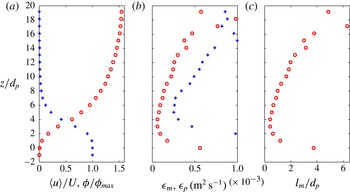
(a) Normalised mean streamwise velocity (○) and concentration profiles (
 $+$
). (b) Momentum (○) and concentration (
 $+$
) diffusivities. (c) Mixing length profile.

It must be noted that the momentum diffusivity has a more generic meaning than the eddy viscosity caused by turbulent flow eddies. In fact, it can be anticipated that the momentum diffusivity in the dilute region of the flow will actually correspond to the eddy viscosity where
 $l_{m}$
should follow a linear evolution with
 $z$
. However, in the dense region of the flow the momentum diffusivity will be dominated by intergranular interactions. According to Bagnold (Reference Bagnold1954) the shear stress associated with intergranular interactions in the grain inertia regime is proportional to
 ${\it\rho}_{p}d_{p}^{2}|\text{d}u/\text{d}z|^{2}$
corresponding to a length scale of momentum diffusion controlled by the particle diameter
 $d_{p}$
. A particulate viscosity has also been introduced by Chauchat & Médale (Reference Chauchat and Médale2010) and Chauchat & Médale (Reference Chauchat and Médale2014) for numerical simulations of dry or immersed granular flows based on the dense granular flow rheology
 ${\it\mu}(I)$
. It is noteworthy that the particulate viscosity is expected to diverge in the granular flow region in the quasi-static regime.
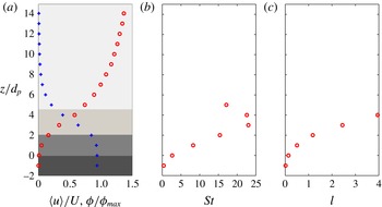
Figure 8 presents the normalised velocity and concentration profiles (a), the vertical evolution of momentum and concentration diffusivities (b) and the vertical profile of mixing length (c). It can be seen that the momentum diffusivity diverges to infinity close to the bed interface, characterising the transition from a fluid-like to a solid-like behaviour. As expected it reaches a minimum corresponding to the inflection point of the velocity profile. For
 $z/d_{p}\gtrsim 5$
, the momentum diffusivity is equivalent to an eddy viscosity and increases linearly with
 $z$
. The concentration diffusivity follows the same trend but is always higher than the momentum diffusivity.
As can be seen in figure 8(c), the mixing length diverges downward for
 $z/d_{p}<2$
, consistently with the momentum diffusivity profile. This indicates that the characteristic length scale associated with momentum diffusion increases dramatically downward. As proposed by Jenkins (Reference Jenkins2007), this behaviour is most probably related to the increase of the length of contact chains when enduring contacts occur between particles. The length scale associated with the contact chain network seems to be the relevant length scale of momentum diffusion in this layer. This suggests that momentum is mainly transferred through permanent or long-term contacts between particles by frictional interactions. In the region
 $2\lesssim z/d_{p}\lesssim 4$
–5, the mixing length reaches a minimum (
 $l_{m}/d_{p}\approx 0.5$
) and is fairly constant. The mixing length is a fraction of the particle diameter in this region which suggests that the granular flow corresponds to the grain inertia regime. This is consistent with the granular shear stress formulation proposed by Bagnold (Reference Bagnold1954). Intuitively, the close agreement between the particle motion scale and their diameter suggests that they interact through collisions. For
 $z/d_{p}\gtrsim 4$
–5, the mixing length profile increases linearly with
 $z$
, consistently with the law of the wall in turbulent shear boundary layers. This observation supports the fact that the large-scale turbulent motions are the dominant momentum diffusion scales in this region.
From this analysis, the position
 $z/d_{p}\approx 4{-}5$
corresponds to the transition between a layer dominated by granular interactions, denoted as the bed layer in the following, and a layer dominated by turbulent processes, denoted as the suspension layer in the following.
In order to make more precise the nature of intergranular interactions in the bed layer, the Stokes and inertial numbers, characterising the granular flow regime, are introduced. Following Armanini et al. (Reference Armanini, Capart, Fraccarollo and Larcher2005)’s definition a Stokes number based on the velocity shear rate is defined as:
 $$\begin{eqnarray}\mathit{St}=\frac{1}{18}\frac{{\it\rho}_{p}}{{\it\rho}_{f}}\frac{d_{p}^{2}\left|\displaystyle \frac{\text{d}u}{\text{d}z}\right|}{{\it\nu}_{f}}.\end{eqnarray}$$
This Stokes number characterises the competition between the deformation rate at the origin of particle fluctuating motions and the viscous effects that damp collisions efficiency. For
 $\mathit{St}\gtrsim 10{-}15$
, the fluctuating motion of particles is no longer influenced by the fluid viscosity and inertial collisions is the dominant mechanism. On the other hand for
 $\mathit{St}\lesssim 10{-}15$
, viscous effects are strong enough to damp collision efficiency and reduce dramatically particle velocity fluctuations (Armanini et al.
Reference Armanini, Capart, Fraccarollo and Larcher2005). Figure 9(b) shows the profile of the Stokes number. The profile shape and the order of magnitude is in good agreement with those obtained by Armanini et al. (Reference Armanini, Capart, Fraccarollo and Larcher2005) for a different particle shape and density. In the present experiment the Stokes number is greater than 10–15 for
 $z/d_{p}\gtrsim 2$
. This confirms that the granular flow in this layer is collisional.
(a) Normalised mean streamwise velocity (○) and concentration profiles (
 $+$
) and representation of the static, frictional, collisional and suspension layers (from dark to light). (b) Stokes number profile. (c) Inertial number profile.

In addition to this first Stokes number a second one is defined as the ratio between a free-fall timescale and a viscous timescale for a particle in a dense granular medium subjected to a particulate pressure
 $P^{p}$
in a fluid of viscosity
 ${\it\nu}_{f}$
(Cassar, Nicolas & Pouliquen Reference Cassar, Nicolas and Pouliquen2005):
 $$\begin{eqnarray}\mathit{St}^{\ast }=\frac{d_{p}}{{\it\nu}_{f}}\sqrt{{\it\rho}_{p}P^{p}}.\end{eqnarray}$$
This Stokes number has been introduced in the framework of the dense granular flow rheology and it allows one to determine whether the timescale of rearrangement is controlled by the fluid viscosity or the particle inertia. The corresponding regimes are the viscous or inertial regimes of the granular flow respectively (Andreotti et al.
Reference Andreotti, Forterre and Pouliquen2013). The particulate pressure
 $P^{p}$
represents the normal stress associated with the granular interactions. Under steady uniform and homogeneous conditions and for concentration values higher than a given critical concentration
 ${\it\phi}_{c}$
, the particulate pressure balances the buoyant weight of particles above a given position
 $z$
such that:
 $$\begin{eqnarray}P^{p}(z)=\left\{\begin{array}{@{}ll@{}}0 & \text{for }z\geqslant z_{c}\\ ({\it\rho}_{p}-{\it\rho}_{f})g\displaystyle \int _{z}^{z_{c}}{\it\phi}(z)\text{d}z & \text{otherwise},\end{array}\right.\end{eqnarray}$$
where
 $z_{c}$
is the vertical position at which
 ${\it\phi}={\it\phi}_{c}$
. In the present case we have set the critical concentration
 ${\it\phi}_{c}=0.08$
corresponding to an inter-particle distance of one particle diameter. This value is commonly used as the transition below which intergranular stresses cannot be neglected (e.g. Hsu et al.
Reference Hsu, Jenkins and Liu2004). This criterion corresponds here to the position
 $z_{c}/d_{p}\approx 5$
, which is in good agreement with the transition found on the basis of momentum diffusivity analysis (figure 8). This further confirms that this position represents a transition between the bed and suspension layers. One must note that (3.13) is valid only if granular interactions are the only processes at work inside the bed layer and that the buoyant weight of particles is entirely supported by intergranular normal stress, i.e. turbulent effects do not participate in particle dispersion for
 $z/d_{p}<5$
. Based on this estimate of the particulate pressure the value of
 $\mathit{St}^{\ast }$
is always larger than
 $10^{2}$
in the bed layer, indicating that the granular flow is in the inertial regime and that the dense granular flow rheology is governed by the inertial number
 $I$
defined as:
 $$\begin{eqnarray}I=\frac{d_{p}\left|\displaystyle \frac{\text{d}u}{\text{d}z}\right|}{\sqrt{P^{p}/{\it\rho}_{p}}}.\end{eqnarray}$$
The inertial number can be interpreted as the ratio between the vertical timescale of rearrangement and the horizontal timescale of deformation (Andreotti et al.
Reference Andreotti, Forterre and Pouliquen2013). For
 $I\approx 0$
the granular flow is in the quasi-static regime. For
 $I\gtrsim 1$
, the granular flow is in the gaseous regime in which binary collisions are dominant (Forterre & Pouliquen Reference Forterre and Pouliquen2008). In between these two values the granular flow is in the liquid regime where both frictional and collisional interactions control the flow behaviour.
In figure 9(c) the vertical profile of the inertial number is presented. One can observe that
 $I$
increases from zero to one between
 $z/d_{p}=0$
and
 $z/d_{p}\approx 2$
. For
 $z/d_{p}>2$
,
 $I$
still increases and reaches values greater than unity. This is in agreement with the conclusions reached by Armanini et al. (Reference Armanini, Capart, Fraccarollo and Larcher2005) and Capart & Fraccarollo (Reference Capart and Fraccarollo2011) that in the lower part of the bed layer frictional interactions are dominant whereas in the upper layer binary collisions are dominant. The thickness of the frictional layer of approximately
 $2d_{p}$
observed in the present experiment is in good agreement with the measurements of Capart & Fraccarollo (Reference Capart and Fraccarollo2011) for the same Shields number.
To summarise the main findings presented in this subsection, it has been shown that a transition from a suspension layer dominated by turbulent mechanisms to a bed layer dominated by granular interactions occurs around
 $z/d_{p}\approx 4{-}5$
. The bed layer can be divided into two sublayers, an upper layer in which binary collisions dominate the vertical transfer of momentum and a lower layer in which frictional interactions dominate (see figure 9
a). Furthermore, for a suspension number around unity the solid load is equipartitioned between the bed layer and the suspension layer.
3.3. Turbulent processes in the suspension layer
In this subsection, the modulation of turbulent momentum mixing efficiency due to the presence of particles is first considered by comparing the direct mixing length estimation to different formulations taking into account sediment effects. Second, the concentration profile obtained from a Rouse model is compared with the one measured in the suspension layer.
3.3.1. Mixing length profile
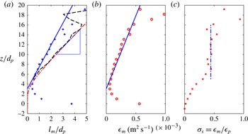
Figure 10(a) shows the mixing length profile deduced from the experimental measurements. As mentioned previously the mixing length is linear in
 $z$
for
 $z/d_{p}\in [5;14]$
and can be approximated by the following expression:
 $$\begin{eqnarray}l_{m}(z)={\it\kappa}^{SF}(z-z_{d}),\end{eqnarray}$$
in which the von Karman parameter
 ${\it\kappa}^{SF}=0.225$
and the mixing length origin
 $z_{d}=3.1d_{p}$
have been determined from a best fit. The solution is represented by a solid line in figure 10(a). The obtained value of
 ${\it\kappa}^{SF}$
is significantly lower than the value obtained in clear-water turbulent boundary layers (
 ${\it\kappa}^{cw}=0.41$
). This feature is representative of a strong turbulence damping induced by the presence of particles as previously observed by Vanoni (Reference Vanoni1975), Best et al. (Reference Best, Bennett, Bridge and Leeder1997), Amoudry, Hsu & Liu (Reference Amoudry, Hsu and Liu2008) and Gaudio, Miglio & Dey (Reference Gaudio, Miglio and Dey2010) amongst others. It is noteworthy that the mixing length slope remains as low in the upper water column where the local concentration values are particularly low. This suggests that the effect of particles in the lower part affects the mixing length associated with turbulent eddies over a large fraction of the boundary layer, even in regions where the concentration is almost zero. This supports the presence of non-local effects induced by the sheet-flow layer.
(a) Mixing length profiles: measured (
 $+$
), linear fit (——), result of (3.16) (- - -) and result of (3.18) (— ⋅ —
 $\!$
). The coefficient of determination of the linear fit is
 $R^{2}=0.984$
. The slope 0.41 is represented by the blue triangle. (b) Profile of measured momentum diffusivity (○) and linear fit obtained from the mixing length linear fit (——). (c) Ratio between the momentum and concentration diffusivity (
 $\times$
); the vertical dot-dashed line corresponds to the Schmidt number value and the associated standard deviation is 0.05.

From a modelling point of view, the turbulence damping induced by the presence of particles in sediment-laden flows has been classically considered via stratification effects (Villaret & Trowbridge Reference Villaret and Trowbridge1991). The same conceptual approach has been applied in several sheet-flow models to account for turbulence damping effects (Jenkins & Hanes Reference Jenkins and Hanes1998; Capart & Fraccarollo Reference Capart and Fraccarollo2011; Berzi & Fraccarollo Reference Berzi and Fraccarollo2013). In this approach, a correction depending on the Richardson number is introduced as:
 $$\begin{eqnarray}l_{m}^{Ri}=\sqrt{1-{\it\phi}}\left(1-7\mathit{Ri}\right){\it\kappa}^{cw}(z-z_{d}),\end{eqnarray}$$
where a shifted vertical axis
 $z-z_{d}$
is used consistently with the best-fit method applied previously. The Richardson number characterises the competition between turbulence production induced by shearing and turbulence damping induced by density stratification as:
 $$\begin{eqnarray}\mathit{Ri}={\displaystyle \frac{-{\displaystyle \frac{g}{{\it\rho}_{m}}}{\displaystyle \frac{\text{d}{\it\rho}_{m}}{\text{d}z}}}{\left|{\displaystyle \frac{\text{d}u}{\text{d}z}}\right|^{2}}}.\end{eqnarray}$$
The Richardson number decreases quite linearly from
 $\mathit{Ri}=0.09$
at
 $z/d_{p}=0$
to
 $\mathit{Ri}=0.01$
at
 $z/d_{p}=15$
(not shown here). The resulting mixing length profile (equation (3.16)) is shown in figure 10(a) (dashed line). It can be seen that this formulation underestimates the damping effect because the resulting mixing length profile is larger than the measured one. Furthermore, as the correction factor is restricted to local stratification effects, which are very low above
 $z/d_{p}\approx 5$
, it cannot account for the non-local effects supported by the direct mixing length measurement. This is illustrated by the fact that the slope of the modelled mixing length reaches the clear-water value 0.41 immediately above the bed layer. The von Karman parameter used in formulation (3.16) has been taken at its clear-water value as it is classically done in a priori modelling approaches.
The empirical formulation used by Revil-Baudard & Chauchat (Reference Revil-Baudard and Chauchat2013) in their two-phase sheet-flow model, relates the mixing length to the integral of the concentration profile according to:
 $$\begin{eqnarray}l_{m}^{{\it\phi}}={\it\kappa}^{cw}\int _{-\infty }^{z}\frac{{\it\phi}^{m}-{\it\phi}}{{\it\phi}^{m}}\text{d}z.\end{eqnarray}$$
This formulation is a first-order model approximation taking into account non-local effects. The corresponding profile is represented by the dash–dotted line in figure 10(a). An interesting aspect of this simple model is that unlike (3.16) no reference of the bed level position is required, as long as the concentration profile is known. It can be seen on figure 10(a) that the integral of the concentration profile slightly modifies the slope of the modelled mixing length up to the position
 $z/d_{p}\approx 7$
. However, the modelled mixing length values are also overestimated compared to the direct estimation, suggesting that this first-order approach is not sufficiently accurate without tuning the von Karman parameter.
It appears that the modification of the mixing length in regions where the concentration and the stratification are negligibly low implies that more refined turbulence models are required.
3.3.2. Concentration profile
The analytical expression for the concentration profile in the suspension layer can be obtained from the sediment mass balance (see (3.7) Rouse Reference Rouse1937). The upward turbulent dispersion flux is modelled by a concentration diffusivity
 ${\it\epsilon}_{p}$
, related to the momentum diffusivity by the introduction of a Schmidt number
 ${\it\sigma}_{s}$
as:
 ${\it\epsilon}_{p}={\it\epsilon}_{m}/{\it\sigma}_{s}$
.
The Schmidt number corresponding to the ratio between the momentum diffusivity and the concentration diffusivity is shown in figure 10(c). The ratio increases from zero at the bed interface to a fairly constant value of
 ${\it\sigma}_{s}=0.44$
for
 $z/d_{p}\gtrsim 5$
. The region of constant Schmidt number value confirms the validity of the proportionality between the concentration diffusivity and the eddy viscosity assumed in the Rouse formulation. The systematic uncertainty in the Schmidt number is dominated by the dispersion in the settling velocity estimations (see (3.8)). It is evaluated at 20 %, even though no size segregation has been observed in the suspension.
Using the linear fit of the mixing length profile (3.15), the profile of momentum diffusivity in the suspension layer (see figure 10 b) can be expressed as:
 $$\begin{eqnarray}{\it\epsilon}_{m}=u_{\ast }{\it\kappa}^{SF}(z-z_{d}).\end{eqnarray}$$
Substituting this relationship in (3.7) the sediment volume balance can be written as:
 $$\begin{eqnarray}{\displaystyle \frac{\text{d}{\it\phi}}{\text{d}z}}-{\displaystyle \frac{p}{(z-z_{d})}}{\it\phi}=0,\end{eqnarray}$$
where
 $p=-({\it\sigma}_{s}w_{s}/{\it\kappa}^{SF}u_{\ast })$
is the Rouse number as defined by Nielsen & Teakle (Reference Nielsen and Teakle2004). Equation (3.20) is a first-order ordinary differential equation in
 $z$
that can be integrated analytically from a given elevation
 $z_{r}$
at which the concentration
 ${\it\phi}(z_{r})={\it\phi}_{r}$
is known. This leads to the well-known Rouse profile:
 $$\begin{eqnarray}{\it\phi}(z)={\it\phi}_{r}\left(\frac{z-z_{d}}{z_{r}-z_{d}}\right)^{p}.\end{eqnarray}$$
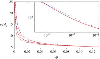
Figure 11 shows the comparison between the concentration profile predicted by (3.21) using
 ${\it\sigma}_{s}=0.44\pm 0.088$
,
 ${\it\kappa}^{SF}=0.225$
,
 $z_{d}/d_{p}=3.1$
,
 ${\it\phi}_{r}=0.12$
and
 $z_{r}/d_{p}=5$
and the measurements of
 ${\it\phi}(z)$
. The good agreement observed in this figure confirms the validity of an equilibrium between the settling flux and the turbulent dispersion flux in the suspension layer. However, one must keep in mind that (i) a model is required to predict the von Karman parameter and the Schmidt number values, (ii) a reference concentration is needed and (iii) the profile strongly depends on the position of the vertical axis origin. The definition of this origin deserves a particular attention for a suspension layer in the presence of a thick sheet layer.
Comparison between measured (
 $+$
) and modelled suspension profiles using
 ${\it\sigma}_{s}=0.44$
(solid line),
 ${\it\sigma}_{s}=0.528$
(dotted line) and
 ${\it\sigma}_{s}=0.352$
(dashed line).

3.4. Granular processes in the bed layer
In the following, the
 ${\it\mu}(I)/{\it\phi}(I)$
rheology (Forterre & Pouliquen Reference Forterre and Pouliquen2008) is compared with the measurements obtained in the bed layer. The local value of the inertial number ((3.14) and figure 9
c) is used to model the friction coefficient:
 $$\begin{eqnarray}{\it\mu}(I)={\it\mu}_{s}+{\displaystyle \frac{{\rm\Delta}{\it\mu}}{I_{0}/I+1}},\end{eqnarray}$$
where
 ${\it\mu}_{s}$
represents the static friction coefficient, the so-called tangent of the angle of repose, which has been determined experimentally herein (
 ${\it\mu}_{s}=0.7$
see table 1),
 ${\rm\Delta}{\it\mu}$
is the difference between the static and dynamical friction coefficients and
 $I_{0}$
is a phenomenological parameter of the rheology. These parameters are set to
 ${\rm\Delta}{\it\mu}=0.3$
and
 $I_{0}=0.3$
, valid for dry granular flows of glass beads in the inertial regime. These values are also consistent with the ones used in the two-phase sheet-flow model proposed by Revil-Baudard & Chauchat (Reference Revil-Baudard and Chauchat2013).
Concerning the concentration profile, the
 ${\it\phi}(I)$
formulation is given by:
 $$\begin{eqnarray}{\it\phi}(I)={\displaystyle \frac{{\it\phi}^{m}}{1+I}}.\end{eqnarray}$$
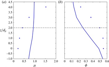
Figure 12(a) shows the comparison between the friction coefficient
 ${\it\mu}={\it\tau}/P^{p}$
estimated from the measurements and the results from (3.22). The measurements indicate that
 ${\it\mu}$
increases with
 $z$
from a static value of
 ${\it\mu}\approx 0.2$
at
 $z/d_{p}=0$
to a value of
 ${\it\mu}\approx 1.5$
at
 $z/d_{p}=4$
. The friction coefficient at the bed interface is much lower than the expected value of
 ${\it\mu}_{s}=0.7$
. Such a difference has already been observed for a laminar bed load of spherical particles but in a smaller proportion (Aussillous et al.
Reference Aussillous, Chauchat, Pailha, Médale and Guazzelli2013). This discrepancy will be discussed in the next section. Moreover, the friction coefficient exceeds unity and keeps increasing until the top of the bed layer while the
 ${\it\mu}(I)$
law predicts a saturation at
 ${\it\mu}={\it\mu}_{s}+{\rm\Delta}{\it\mu}\approx 1$
. A friction coefficient greater than one suggests that other mechanisms than contact interactions contribute to the shear stress. Boyer, Guazzelli & Pouliquen (Reference Boyer, Guazzelli and Pouliquen2011) have observed a similar behaviour when analysing their rheometer data of dense suspension. The authors suggested that the difference between the overall friction coefficient and the friction coefficient associated with contact interactions is due to hydrodynamic interactions linked to lubrication. In the present case, values of the friction coefficient greater than one are more likely to be associated with inter-particle collisions and/or turbulent velocity fluctuations. At this stage of the analysis, the origin of this point remains unclear.
Comparison between measurements (
 $+$
) and prediction from the granular rheology
 ${\it\mu}(I)/{\it\phi}(I)$
(——) for the friction coefficient profile (a) and the concentration profile (b). The horizontal dashed line represents the position for which
 $I=1$
.

Figure 12(b) shows the comparison of the concentration profile predicted by (3.23) with the measurements. The agreement is rather poor and no concentration shoulder is observed, contrary to the model prediction of Hsu et al. (Reference Hsu, Jenkins and Liu2004) based on a kinetic theory approach or of Revil-Baudard & Chauchat (Reference Revil-Baudard and Chauchat2013) based on the granular flow rheology.
These discrepancies between the granular flow rheology and the measurements raise a number of questions: is the particulate pressure estimation based on the concentration profile valid? Are the assumptions of the granular rheology approach satisfied under sheet-flow conditions? Concerning the particulate pressure, the estimate relies on the validity of the measured concentration profile in the denser part of the flow. Also, the momentum balance between intergranular interactions and gravity inside the bed layer is based on the assumption that turbulent dispersion effects are negligible inside the bed layer. This is probably too strong an assumption. Finally, the actual value of the critical volume fraction
 ${\it\phi}_{c}$
is also subject to uncertainties. The choice of
 ${\it\phi}_{c}=0.08$
maximises the particulate pressure which can induce an underestimation of the friction coefficient. However, the factor of more than three observed for
 ${\it\mu}$
at the fixed bed interface cannot be explained solely by this uncertainty.
4. Discussion
This section discusses the validity of the steadiness assumption on which the granular rheology is based and it further interprets the modification of the von Karman and Schmidt numbers.
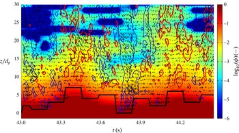
Time evolution of the measured bed interface position (black thick line) and concentration measurements (colourplot in base-10 logarithm) associated to coherent structures detection: the red and blue contours represent the ejections and sweeps respectively as iso-contours of
 $H=2$
as evaluated in Mignot et al. (Reference Mignot, Hurther and Barthelemy2009). The vector plot represents the instantaneous 2C velocity fluctuations.

4.1. Intermittency of the bed layer
An important assumption in the dense granular flow rheology is the steadiness of the granular flow at scales larger than the grain scale. The results presented above are based on average quantities consistently with this hypothesis. The experimental setup is used here to verify this assumption by making use of the high-rate profiling of velocity and concentration as provided by the ACVP technology. Figure 13 shows an example of the time evolution of the ACVP measurements over a duration of approximately 3 s acquired at a frequency of 78 Hz. As mentioned in § 2, the bed interface detection and the concentration measurements are low-pass filtered at a frequency of 7.8 Hz and 4.9 Hz respectively to guarantee a low bias error. The blue and red solid contours represent isolines of relative turbulent shear stress identified as sweep and ejection events, respectively. The
 $uw$
-quadrant threshold technique of Lu & Willmarth (Reference Lu and Willmarth1973) has been applied here with a threshold value of
 $H=2$
as proposed by Mignot et al. (Reference Mignot, Hurther and Barthelemy2009). The colourplot represents the base-10 logarithm of the concentration and the black solid line represents the detected bed interface position. The 2C vector plot corresponds to the instantaneous field of the 2C time fluctuating velocity. It confirms that the velocity field inside a red and blue delimited contour is oriented in quadrant 2 (ejection) and 4 (sweep) in the (
 $u,w$
) plane, respectively.
This figure illustrates the complex interactions between large-scale coherent flow structures, suspended sediment concentration and the bed interface dynamics. A close examination of this figure reveals that erosion events, corresponding to a drop of the bed level position, are associated to sweep events. In terms of concentration, these erosive events are associated with a reduction of concentration while accretion events, corresponding to an increase of the bed level position, are linked to ejection events inducing an increase of concentration. Intuitively, it can be deduced that sweeps are mainly responsible for momentum diffusion while ejections are mainly responsible for particle dispersion/resuspension. This large-scale turbulence-driven intermittency is also believed to explain why the measured granular rheology deviates from the steady-state rheology. Due to the intermittency under the action of the sweeps events, the dense frictional layer observed in the present experiment can be dominated by turbulent processes for the duration of this event. Indeed, on average the flow in the bed layer is highly concentrated and dominated by granular interactions; however turbulent processes occur on a short duration and are sufficiently dynamic to modify the average values of the concentration and the vertical gradient of streamwise velocity. In other words, the layer decomposition is valid on average but not instantaneously at a given vertical position. Momentum and concentration can be transferred by a succession of frictional, collisional or turbulent mechanisms in a short time period. As this intermittency originates from large-scale turbulence effects, it could explain why the local rheology and the Coulomb failure criterion fail in predicting the measurements.
4.2. Turbulent fluid–particle interactions
4.2.1. Schmidt number modification
The Schmidt number in sediment-laden flows has been the subject of many discussions in the literature over the past few decades (e.g. Ismail Reference Ismail1951; Van Rijn Reference Van Rijn1984). Field and laboratory experiments showed that the Schmidt number value can substantially depart from unity (Graf & Cellino Reference Graf and Cellino2002). Greimann, Muste & Holly (Reference Greimann, Muste and Holly1999) argued that the increased diffusion of large particles (Schmidt number lower than unity) originates from the added diffusive nature of the sediment velocity fluctuations. Nielsen & Teakle (Reference Nielsen and Teakle2004) have argued that finite length effects in the vertical distributions of concentration and momentum can explain the decrease of the Schmidt number for increasing suspension number. The authors showed that the use of a first-order Fickian diffusivity for the concentration is only valid if the characteristic length scale of the concentration distribution is much larger than the one of the momentum distribution. This hypothesis is valid for light particles and small suspension number (
 $S\ll 1$
) with an almost homogeneous distribution of the concentration over the water column. In such conditions the vertical gradient of concentration is sufficiently low to neglect second-order terms in the diffusivity model. However, for massive particles (
 $S>1$
) the vertical gradient of concentration can be very important in the bed region, inducing non-negligible second-order terms in the Fickian derivative approximation. Following Nielsen & Teakle (Reference Nielsen and Teakle2004)’s approach these higher-order terms explain the reduction of the Schmidt number for massive particles. An important aspect is that the Schmidt number presented here is calculated from the measured momentum diffusivity which is significantly affected by the presence of particles. As a consequence, the Schmidt number modulation could be mainly induced by the reduction of the turbulence-driven momentum mixing efficiency. To the best of our knowledge a clear quantitative description of the physical processes responsible for the Schmidt number decrease with particle inertia has not yet been proposed.
4.2.2. Turbulence modulation
Villaret & Trowbridge (Reference Villaret and Trowbridge1991) have suggested that the stratified flow analogy is applicable to turbulent sand suspension flows. However, their model fails to reproduce individual profiles and a dependence on the particle size has been observed. A stratified flow analogy cannot account for the particle size dependence. The authors concluded that the physical processes behind this dependence is unclear. The stratification analogy relies on the assumption that the sediment concentration acts as a passive scalar. Following Ferry & Balachandar (Reference Ferry and Balachandar2001), this assumption is fully satisfied when the particle size is smaller than the Kolmogorov dissipation scale. On the contrary, when the particles are massive and their diameter is larger than the Kolmogorov scale, typically of the order of the integral scale of turbulence, particle inertia cannot be neglected and sediment concentration can no longer be considered as a passive scalar. In such conditions density stratification is insufficient to account for the complex interactions between the turbulent fluctuating motions of particles and elementary fluid parcels. In our conditions, the particle size is not negligible compared with the integral length scale of turbulence. This can be seen from the mixing length values shown in figure 8(c), considered as a proxy of the local integral scale of turbulence. The values are of the same order of magnitude as the particle diameter
 $d_{p}=3~\text{mm}$
, supporting the invalidity of the passive scalar assumption due to particle inertia effects.
A better understanding of these complex fluid–particle turbulent interactions is obtained on the basis of particle-scale direct numerical simulations (DNS) (e.g. Kidanemariam et al.
Reference Kidanemariam, Chan-Braun, Doychev and Uhlmann2013; Vowinckel, Kempe & Fröhlich Reference Vowinckel, Kempe and Fröhlich2014) in conditions where the particle size is larger than the Kolmogorov length scale. However these approaches are still restricted to low bulk Reynolds numbers
 $O(10^{3})$
compared to the present conditions of
 $O(10^{5})$
. To our knowledge, such numerical studies have not been applied so far to turbulent sheet-flow conditions. The combination of DNS and large-eddy simulations with small-scale datasets obtained from the present experimental configuration should improve our understanding of fluid–particle turbulent interactions in sediment transport problems. These high-resolution experimental and numerical data will also provide guidelines for the improvement of transport equations in turbulence models.
5. Conclusion
A new high-resolution sheet-flow dataset containing velocity, concentration, sediment flux and turbulent shear stress profiles has been presented in this paper. These measurements are used to discuss the validity of sheet-flow properties and to assess different existing modelling approaches considering turbulent and granular processes.
The analysis of momentum and concentration diffusivities, mixing length, and Stokes and inertial number profiles confirms the flow decomposition into different layers proposed in the literature. Consistently with the mean velocity and concentration profiles, the flow can be divided into a dilute suspension layer (
 ${\it\phi}\lesssim 0.1$
) dominated by turbulent mechanisms and a dense bed layer (
 ${\it\phi}\gtrsim 0.1$
) dominated by granular mechanisms. The dense bed layer can be further divided into two sublayers, a dense frictional sublayer capped by a more dilute collisional sublayer.
In the suspension layer, a significant attenuation of the turbulent momentum diffusion efficiency is observed based on a significant reduction of the von Karman parameter compared to the clear-water value. In this layer, the turbulent momentum diffusivity is shown to be proportional to the turbulent concentration diffusivity with an almost constant coefficient of proportionality equal to
 ${\it\sigma}_{s}=0.44$
.
The mixing length in the suspension layer evolves linearly with
 $z$
as in a clear-water shear boundary layer but the origin of the linear mixing length profile is located in the bed layer, i.e. above the bed interface. Models are necessary for both the prediction of the von Karman parameter and the origin of the modified law of the wall in sheet-flow conditions. Furthermore, the measurements showed that the turbulent momentum diffusion is affected by the solid transport in regions where the concentration and the stratification are negligible. This behaviour strongly supports the existence of non-local effects attributed to the presence of the sheet-flow layer.
The validity of the Rouse model in the suspension layer has been confirmed when all the required parameters are evaluated properly: the von Karman parameter, the Schmidt number, the shifted origin for the
 $z$
axis and the reference concentration value and location.
It has also been shown that the dense granular rheology cannot be applied straightforwardly to predict the measurements in the bed layer. In particular, the Coulomb failure criterion, which is commonly used in the models from the literature, is found to be much lower than the tangent of the measured angle of repose which is classically used in sheet-flow models. This might be explained by the bed layer intermittency attributed to the impact of large-scale coherent flow structures. This large-scale-induced intermittency questions the relevance of a steady-state local rheology and supports the need to include intermittency effects in sheet-flow models.
Acknowledgements
The authors acknowledge the DGA for the financial support of the first author’s PhD thesis (no. 2011-170914/DGA/DS/MRIS). The development of the ACVP has been funded by the EU project Hydralab IV-WISE (contract 261520) and the experiments have been funded by the pole SMINGUE UJF/INPG and SEI-MEPIERA. The authors also gratefully acknowledge J. M. Barnoud for the technical support during the development of the experimental setup.