





1. Introduction
Many fluid mechanical problems involve the motion of solid particles in low-Reynolds-number flows. Examples include the processing of two-dimensional materials (Kamal et al. Reference Kamal, Gravelle and Botto2020; Silmore et al. Reference Silmore, Strano and Swan2021) and polymers (Smith et al. Reference Smith, Babcock and Chu1999), swimming of microorganisms (Lauga & Powers Reference Lauga and Powers2009; Gaffney et al. Reference Gaffney, Dalwadi, Moreau, Ishimoto and Walker2022), mass transport near ciliated surfaces (Selvan et al. Reference Selvan, Duck, Pihler-Puzović and Brumley2025) and numerous applications in microfluidics; see, e.g. Cappello et al. (Reference Cappello, Bechert, Duprat, du Roure, Gallaire and Lindner2019).
Unless the background flow is a pure straining flow, velocity gradients imply the presence of vorticity, a measure of the rotation of infinitesimal material line elements in the fluid. In general, solid particles immersed in such a flow do not simply inherit this rate of rotation from the flow but undergo a more complex motion. In an unbounded Stokes flow the behaviour of rigid particles is encoded in their resistance/mobility matrix whose entries are completely determined by the particles’ shape; see, e.g. Brenner (Reference Brenner1963), Happel & Brenner (Reference Happel and Brenner1983) and Kim & Karrila (Reference Kim and Karrila1991). The particles’ behaviour tends to become increasingly complex as their degree of symmetry is reduced. For instance, in a simple shear flow (with spatially and temporally constant vorticity; the flow of interest in this paper), spherical particles are the only particles that rotate with the local vorticity of the flow. Ellipsoidal particles undergo a periodic rotation (with their orientation following the so-called Jeffery orbits) and translate in the direction of the shear flow. Their rate of rotation varies with their instantaneous orientation relative to the direction of the flow (Jeffery Reference Jeffery1922). This behaviour is, in fact, generic for any rigid axisymmetric particle: Bretherton (Reference Bretherton1962) showed that in a simple shear flow all particles of this type follow the Jeffery orbits of an equivalent ellipsoid. However, when the axisymmetry is broken, the particles exhibit increasingly complex behaviour including the development of quasi-periodic or even chaotic orbits (Yarin et al. Reference Yarin, Gottlieb and Roisman1997; Thorp & Lister Reference Thorp and Lister2019). The particles’ rotation can also be accompanied by a net drift either in the direction of the vorticity (e.g. for helicoidal particles; see Ishimoto Reference Ishimoto2020), or across the streamlines (e.g. for curved fibres; see Wang et al. Reference Wang, Tozzi, Graham and Klingenberg2012).
Further complexity arises in the case of long, slender bodies, such as fibres, whose large aspect ratio makes them easy to deform, often resulting in a strong interaction between the fluid flow and the now evolving particle shape. We refer to du Roure et al. (Reference du Roure, Lindner, Nazockdast and Shelley2019) for a very comprehensive review of the subject. Briefly, such fibres are prone to flow-induced buckling and bending instabilities (Becker & Shelley Reference Becker and Shelley2001; Chakrabarti et al. Reference Chakrabarti, Liu, LaGrone, Cortez, Fauci, du Roure, Saintillan and Lindner2020; Żuk et al. Reference Żuk, Słowicka, Ekiel-Jeżewska and Stone2021; Słowicka et al. Reference Słowicka, Xue, Sznajder, Nunes, Stone and Ekiel-Jeżewska2022; Kurzthaler et al. Reference Kurzthaler, Brandão, Schnitzer and Stone2023), with the importance of fluid–structure interaction (FSI) controlled by the ratio of the fibre’s bending stiffness to the hydrodynamic forces exerted by the flow (Liu et al. Reference Liu, Chakrabarti, Saintillan, Lindner and du Roure2018). Elasticity of these fibres is often modelled using the inextensible Euler–Bernoulli beam theory (Liu et al. Reference Liu, Chakrabarti, Saintillan, Lindner and du Roure2018, Reference Liu, Sznajder and Ekiel-Jeżewska2024), although other frameworks exist, for example, bead–spring models in which the fibres are represented as a series of small hydrodynamically interacting spheres (beads) connected by flexible springs (Żuk et al. Reference Żuk, Słowicka, Ekiel-Jeżewska and Stone2021; Słowicka et al. Reference Słowicka, Xue, Sznajder, Nunes, Stone and Ekiel-Jeżewska2022). Fully deformable elastic fibres are also commonly approximated using a composite shape consisting of straight and rigid slender arms joined by torsional springs (Hu et al. Reference Hu, Zhang and Shelley2022; Roggeveen & Stone Reference Roggeveen and Stone2025).
Similarly to their rigid counterparts, elastic fibres in shear flows typically rotate, often following Jeffery-like orbits while undergoing large-amplitude time-periodic deformations (Roggeveen & Stone Reference Roggeveen and Stone2025). In certain regimes chaotic behaviour is observed (Słowicka et al. Reference Słowicka, Wajnryb and Ekiel-Jeżewska2015). The fibres tend to either orient themselves in the plane of shear or align with the direction of vorticity (Słowicka et al. Reference Słowicka, Stone and Ekiel-Jeżewska2020) and the rotation can again be accompanied by a cross-streamline drift (Słowicka et al. Reference Słowicka, Wajnryb and Ekiel-Jeżewska2015).
In all the examples discussed so far the shear flow causes the particles to rotate. However, it is also possible to construct particles that adopt steady orientations relative to the shear flow while drifting steadily across the streamlines; see, e.g. Brenner (Reference Brenner1964) or Borker et al. (Reference Borker, Stroock and Koch2018). Arguably the simplest such particle was recently studied by Roggeveen & Stone (Reference Roggeveen and Stone2022) who considered the motion of a boomerang-shaped slender rigid fibre in a simple shear flow. Modelling the traction on the fibre by slender-body theory (Batchelor Reference Batchelor1970; Cox Reference Cox1970; Johnson Reference Johnson1980), they established the range of geometric parameters (the fibre’s opening angle and the length ratio of its two arms) for which the fibre rotates or adopts a steady orientation. Fibres that adopted a steady orientation were found to drift steadily across the streamlines. Conversely, those that performed the equivalent of Jeffery orbits were found to be advected by the shear flow with a zero net drift, implying that a shear flow can separate a dilute suspension of such fibres, depending on their geometry and elasticity.
Since slender fibres are easily deformed by the fluid traction, it is natural to ask two questions: (i) Under what conditions do the elastic counterparts of the fibres studied by Roggeveen & Stone (Reference Roggeveen and Stone2022) display an equivalent behaviour? (ii) What is the role of FSI in the transition between rotating and non-rotating states? It is the aim of the current paper to address these questions. For this purpose, § 2 reviews Roggeveen & Stone’s (Reference Roggeveen and Stone2022) set-up and then extends it to incorporate FSI by coupling slender-body theory with a Kirchhoff–Love model to describe the flow-induced deformation of an arbitrarily shaped fibre in the shear flow. We outline the general structure of the different types of solutions (representing rotating and non-rotating states) in § 3 before describing the numerical method used to compute the solutions in § 4. In the latter section we also derive the eigenvalue problem that determines the stability of the non-rotating states. In § 5, we present our results, starting with the case of the elastic equivalent of Roggeveen & Stone’s (Reference Roggeveen and Stone2022) boomerang-shaped fibres. We demonstrate that for these fibres non-rotating states continue to exist for a wide range of the parameter that characterises the strength of the FSI. We show that in the presence of FSI the structure of the solutions becomes significantly more complicated than for the rigid case. We then analyse the nature of the transition from non-rotating to rotating states and show that this transition occurs via a degenerate sniper bifurcation. In § 5.2 we illustrate the generality of our results by demonstrating that the behaviour observed for boomerang-shaped fibres is also displayed for a variety of other fibre shapes. We summarise our findings in § 6.
2. The model
2.1. Rigid fibres
Figure 1 shows a sketch of the problem set-up: an arbitrarily shaped fibre of circular cross-section (radius
 $a$
and total length
 $\mathcal{L}$
) is advected by a viscous fluid of viscosity
 $\mu$
. In the absence of the fibre, the flow is a steady shear flow with shear rate
 $\dot {\gamma }$
, the axis of vorticity being aligned with the
 $x_3$
-direction. We assume that the fibre is and remains in the
 $(x_1,x_2)$
-plane. Unit vectors in the coordinate directions are denoted by
 $\boldsymbol {e}_i \ (i=1,2,3)$
.
Sketch of the problem set-up: an arbitrarily shaped fibre is immersed in a shear flow,
 $\boldsymbol{U}^\infty$
. The fibre’s rigid-body motion is described by the position vector
 $\boldsymbol{r}_{{b}}(t)$
to a material reference point, and the angle
 $\theta (t) \in [0,2\pi ]$
between the unit tangent to the fibre at this point and the
 $x_1$
-axis. The position vector to a material point on the fibre,
 $\boldsymbol {R}(\zeta ,t)$
, is parametrised by a Lagrangian coordinate
 $\zeta$
. The vector
 $\boldsymbol{e}_{{t}}$
is the unit tangent to the fibre and the vector
 $\boldsymbol{f}_{\!\!{f}}$
represents the fluid traction acting on the fibre. Thin open arrows indicate the direction in which coordinates increase; thick filled arrows represent vectors.

Figure 1. Long description
A sketch of the problem setup involving an arbitrarily shaped fiber immersed in a shear flow. The fiber’s rigid-body motion is described by the position vector to a material reference point and the angle between the unit tangent to the fiber at this point and the x1-axis. The position vector to a material point on the fiber is parametrized by a Lagrangian coordinate. The vector et represents the unit tangent to the fiber, and the vector ff represents the fluid traction acting on the fiber. Thin open arrows indicate the direction in which coordinates increase, and thick filled arrows represent vectors.
We non-dimensionalise all lengths on the total length of the fibre,
 $\mathcal{L}$
, time on the inverse shear rate,
 $\dot {\gamma }^{-1}$
, and all velocities on the associated natural scale,
 $\mathcal{L}\dot {\gamma }$
. Where needed, asterisks are used to distinguish dimensional quantities from their non-dimensional equivalents.
We describe the position and orientation of the fibre in terms of the non-dimensional position vector
 $\boldsymbol {r}_{{b}}(t) = (X(t),Y(t))$
to some material reference point on the fibre, and the angle
 $\theta (t)$
that the unit tangent to the fibre,
 $\boldsymbol {e}_t$
, at this point makes with the
 $x_1$
-axis. We also introduce a non-dimensional Lagrangian coordinate
 $\zeta \in [0,1]$
which labels material points along the fibre, so that the position vector to a point on the fibre is given by
 $\boldsymbol {R}(\zeta ,t)$
, which for a rigid fibre is easily expressed in terms of
 $\boldsymbol {r}_{{b}}(t)$
and
 $\theta (t)$
; see (2.9) below. (In cases where the reference point is located at a coordinate
 $\zeta _{\textit{ref}}$
at which the fibre has a kink (as for the boomerang shape), we measure the orientation using the tangent
 $\boldsymbol {e}_t$
obtained when approaching
 $\zeta _{\textit{ref}}$
from above.)
Assuming that the fibre has a large aspect ratio,
 $\mathcal{L}/a \gg 1$
, and that the flow is dominated by viscous effects, the non-dimensional traction,
 $\boldsymbol {f}_{\!\!{f}}$
, that the fluid exerts onto the fibre can be approximated by slender-body theory (see, e.g. Batchelor Reference Batchelor1970; Cox Reference Cox1970; Johnson Reference Johnson1980), as
 \begin{equation} \boldsymbol{f}_{\!\!{f}}= \frac {\boldsymbol{f}^*_{\!\!{f}}}{c_\perp {\mathcal{L}}\dot {\gamma }} = \left (\boldsymbol{I}-\frac {1}{2}\boldsymbol{e}_{{t}}\boldsymbol{e}_{{t}}\right )\boldsymbol{\cdot }\left (\boldsymbol{U}^{\infty }-\frac {\partial \boldsymbol {R}}{\partial t}\right )\!. \end{equation}
Here,
 $c_\perp =4\pi \mu /\ln ({\mathcal{L}}/a)$
is the drag coefficient,
 $\boldsymbol {e}_{{t}}$
is the unit tangent to the fibre,
 $\boldsymbol {U}^{\infty } = x_2 \boldsymbol {e}_1$
is the background shear flow and
 $\partial \boldsymbol {R}/\partial t$
the instantaneous local velocity of the material point on the fibre onto which the traction acts.
Assuming that inertial effects do not affect the dynamics of the fibre, Roggeveen & Stone (Reference Roggeveen and Stone2022) employed (2.1) to compute the fibre’s mobility matrix. This approach is equivalent to imposing that the non-trivial components of the net viscous drag and the torque acting on the fibre vanish so that
 \begin{equation} \boldsymbol{D}=\int _0^1 \boldsymbol{f}_{\!\!{f}}\, \left |\frac {\partial \boldsymbol{R}}{\partial \zeta }\right |\,\textrm{d}\zeta =\boldsymbol{0}, \end{equation}
 \begin{equation} \boldsymbol{T}\boldsymbol{\cdot }\boldsymbol{e}_3=\left \{\int _0^1 \left [(\boldsymbol{R}-\boldsymbol{R}_{{c}})\times \boldsymbol{f}_{\!\!{f}}\,\right ]\, \left |\frac {\partial \boldsymbol{R}}{\partial \zeta }\right |\,\textrm{d}\zeta \right \}\boldsymbol{\cdot }\boldsymbol{e}_3=0. \end{equation}
Here,
 $\boldsymbol {R}_{{c}}$
is the position vector to the fibre’s centre of gravity. However, given that (2.2) imposes
 $\boldsymbol {D} = \boldsymbol {0}$
, we can omit this term or replace
 $\boldsymbol {R}_{{c}}$
by any other vector. For our analysis, the choice
 $\boldsymbol {R}_{{c}}(t) = \boldsymbol { r}_{{b}}(t)$
was found to be the most convenient.
We note that, for straight fibres, slender-body theory predicts a spurious equilibrium orientation at
 $\theta =0$
. This is an artefact of the slender-body limit; a straight fibre of finite thickness would rotate, albeit slowly, through this orientation.
Equations (2.2) and (2.3) represent three scalar ordinary differential equations (ODEs) that determine the evolution of
 $\boldsymbol {r}_{{b}}(t)$
and
 $\theta (t)$
.
Roggeveen & Stone (Reference Roggeveen and Stone2022) applied a variant of this approach (based on a mathematically equivalent mobility-matrix formalism) to the special case where the fibre comprises two straight, rigid arms whose length ratio they characterised by the parameter
 $q \in [0,1/2)$
so that the short and long arms of the fibre have lengths
 $(1/2-q)\mathcal{L}$
and
 $(1/2+q)\mathcal{L}$
, respectively. The two rigid arms formed a boomerang-shaped fibre with an opening angle
 $\alpha$
. Roggeveen & Stone (Reference Roggeveen and Stone2022) showed, for wide a range of the geometric parameters
 $q$
and
 $\alpha$
, that the equations have solutions for which
 $\theta (t) = \theta _{{eq}} = const.$
, implying that the fibre retains a constant orientation, despite the presence of vorticity in the background flow. This is illustrated in figure 2(a) where the grey region shows the range of
 $(q,\alpha )$
values for which such steady orientations exist. The boundary of that region was obtained from the numerical solution of (2.2) and (2.3) (see below for details); the dashed red line shows the analytical prediction from Roggeveen & Stone (Reference Roggeveen and Stone2022).
For each pair of
 $q$
and
 $\alpha$
in this grey region, the fibre has four possible equilibria, two of which are stable and two unstable. These orientations are illustrated in the conceptual sketch in figure 2(b). The angles associated with the two stable/unstable orientations differ by an angle of
 $\pi$
. When the fibre is in this steady orientation it drifts across the streamlines with a constant vertical speed in the direction indicated by the arrows in figure 2(b); see below for more details.
(a) Plot of the
 $(q,\alpha )$
parameter space, with the grey region indicating parameters for which the rigid boomerang-shaped fibres considered by Roggeveen & Stone (Reference Roggeveen and Stone2022) adopt constant orientations; elsewhere they rotate while following Jeffery orbits. For each pair of
 $q$
and
 $\alpha$
in the grey region the fibre can adopt four equilibrium orientations. (b) Illustration of equilibrium orientations: two of the orientations are unstable, two are stable. The stable and unstable pairs differ by an angle of
 $\pi$
. While in their equilibrium orientations the fibres drift across the streamlines, with the direction of the drift indicated by the arrows. Note that the figure closely mirrors and has been directly inspired by figures 4 and 5 of Roggeveen & Stone (Reference Roggeveen and Stone2022) whose analytical predictions for the boundary of the grey region are shown by the red dashed line in (a).

2.2. Extension to elastic fibres
2.2.1. Modelling the elastic fibres
To extend the analysis of Roggeveen & Stone (Reference Roggeveen and Stone2022) to the case of elastic fibres, we model the fibre as a Kirchhoff–Love beam with extensional stiffness
 ${\mathcal{E}} = \pi a^2 E$
and bending stiffness
 ${\mathcal{B}} = ({1}/{4})\pi a^4 E$
, where
 $E$
is the fibre’s effective one-dimensional Young’s modulus.
Sketch illustrating the deformation, displacement and rotation of an arbitrarily shaped fibre in viscous flow. The dashed red line, parametrised by
 $\boldsymbol{r}_0(\zeta )$
, where
 $\zeta$
is a Lagrangian coordinate, shows the undeformed fibre, clamped at the origin of the
 $(x_1,x_2)$
coordinate system. When loaded by the quasi-steady traction
 $\boldsymbol {f}_{\kern-1pt s}$
, the fibre deforms into the shape given by
 $\boldsymbol{R}_0(\zeta )$
, shown by the solid red line. In addition to the deformation, the fibre is subject to a rigid-body translation by
 $\boldsymbol { r}_b(t)$
and a rotation so that the unit tangent to the fibre at its material reference point forms an angle
 $\theta (t)$
with the
 $x_1$
-axis. In this configuration, the deformed fibre (black) is parametrised by the vector
 $\boldsymbol {R}(\zeta ,t)$
and is subject to the fluid traction,
 $\boldsymbol {f}_{\kern-1pt s}$
.

In its undeformed, stress-free state we position the fibre so that the material reference point coincides with the origin of the Cartesian coordinate system
 $(x_1,x_2)$
. Furthermore, we orient the fibre so that the unit tangent
 $\boldsymbol {e}_t$
, evaluated at the material reference point (and approaching the reference point from larger values of
 $\zeta$
in cases where the fibre has a kink), is aligned with the
 $x_1$
-axis. The stress-free, undeformed shape of the fibre (represented by the dashed red line in figure 3) is then described by the vector
 $\boldsymbol {r}_0(\zeta )$
, where
 $\zeta \in [0,1]$
is the non-dimensional Lagrangian coordinate. When subjected to a quasi-steady traction
 $\boldsymbol {f}_{\!{s}}^*$
, the fibre deforms so that the non-dimensional position vector to its centreline changes to
 $\boldsymbol {R}_0(\zeta )$
, shown by the solid red line in figure 3. The fibre’s deformation is determined by the principle of virtual displacements (see, e.g. Wempner Reference Wempner1973)
 \begin{equation} \int _{0}^{{1}} \left ( \left (\frac {{\mathcal{E}}{\mathcal{L}}^2}{\mathcal{B}}\right ) \ \gamma \,\delta \gamma + \kappa \delta \kappa - \sqrt {\frac {{\mathcal{A}}}{{\mathcal{a}}}}\ \boldsymbol{f}_{\!{s}} \boldsymbol{\cdot }\delta \boldsymbol{R}_0 \right )\,\sqrt {a}\,\textrm{d}{\zeta }=0. \end{equation}
Since we anticipate the fibre deformation to be dominated by bending effects, we have non-dimensionalised the traction (a force per unit length of the deformed fibre, acting on the deformed fibre) on the bending stiffness, so
 $\boldsymbol {f}_{\!{s}} = \boldsymbol{f}^*_{\!{s}} \mathcal{L}^3/{\mathcal{B}}$
. We note that for thin fibres we have
 ${\mathcal{E}}{\mathcal{L}}^2/{\mathcal{B}} \gg 1$
, implying that the fibre’s extensional stiffness is much larger than its bending stiffness. In (2.4), the quantities
 \begin{equation} {{\mathcal{a}}=\frac {\partial \boldsymbol{r}_0}{\partial \zeta }\boldsymbol{\cdot }\frac {\partial \boldsymbol{r}_0}{\partial \zeta }} \ \ \mbox{ and }\ \ {{\mathcal{A}}=\frac {\partial \boldsymbol{R}_0}{\partial \zeta }\boldsymbol{\cdot }\frac {\partial \boldsymbol{R}_0}{\partial \zeta }} \end{equation}
denote the squares of the lengths of infinitesimal material line elements in the undeformed and deformed configurations, respectively, while the ratio
 $\sqrt {{\mathcal{A}}/{\mathcal{a}}}$
represents the ‘extension ratio’ of the fibre’s centreline. The fibre’s curvature is characterised by
 \begin{equation} {{\mathcal{c}} = \boldsymbol{n}\boldsymbol{\cdot }\frac {d^2\boldsymbol{r}_0}{\textrm{d}\zeta ^2}} \ \ \mbox{and }\ \ {{\mathcal{C}} = \boldsymbol{N}\boldsymbol{\cdot }\frac {\partial ^2\boldsymbol{R}_0}{\partial \zeta ^2}}, \end{equation}
where
 $\boldsymbol {n}$
and
 $\boldsymbol {N}$
are unit normal vectors to the fibre’s undeformed and deformed centrelines, respectively. The ‘
 $1\times 1$
’ strain and bending ‘tensors’
 $\gamma$
and
 $\kappa$
in (2.4) are then given by
 \begin{equation} \gamma =\frac {1}{2}({\mathcal{A}}-{\mathcal{a}}) \ \ \mbox{ and } \ \ \kappa =-({\mathcal{C}}-{\mathcal{c}}). \end{equation}
These measures are geometrically exact and are therefore applicable to arbitrarily large, geometrically nonlinear deformations. The use of a linear constitutive equation (implying a linear relation between the extensional and bending stresses and the strain and bending measures, respectively) in the principle of virtual displacements (2.4) is justified by the fact that the fibre undergoes very small extensions, leading to small overall strains. However, we note that, unlike some other studies of elastic fibres (e.g. Becker & Shelley Reference Becker and Shelley2001; Tornberg & Shelley Reference Tornberg and Shelley2004; Liu et al. Reference Liu, Chakrabarti, Saintillan, Lindner and du Roure2018, Reference Liu, Sznajder and Ekiel-Jeżewska2024), we do not impose inextensibility.
In the reference configuration we subject the fibre to clamped boundary conditions, applied at the reference point, by imposing
 \begin{equation} \boldsymbol{R}_0({\zeta =\zeta _{\textit{ref}}})\boldsymbol{\cdot }\boldsymbol{e}_{{1}}=0,\ \ \boldsymbol{R}_0({\zeta =\zeta _{\textit{ref}}})\boldsymbol{\cdot }\boldsymbol{e}_{{2}}=0,\ \ \ \left . \frac {\textrm{d}\left (\boldsymbol{R}_0\boldsymbol{\cdot }\boldsymbol{e}_{{2}}\right )}{\textrm{d}{\zeta }}\right |_{{{\zeta =\zeta _{\textit{ref}}}}}=0, \end{equation}
where
 $\zeta _{\textit{ref}}$
is the Lagrangian coordinate of the material reference point.
2.2.2. FSI
We now consider how the fluid and solid mechanics are coupled within our model. The dashed red line in figure 3 shows the undeformed fibre in its reference position/orientation. The fluid traction not only deforms the fibre into the shape shown by the solid red line but it also induces a rigid-body motion which displaces the material reference point on the fibre by the vector
 $\boldsymbol {r}_{{b}}$
and rotates the fibre about that point by
 $\theta (t)$
. If the fibre is rigid, its position is therefore given by
 \begin{equation} \boldsymbol {r}\left (\zeta ,t\right ) = \boldsymbol {r}_{{b}}(t) + \textsf {R}\left (\theta (t)\right ) \ \boldsymbol {r}_0\left (\zeta \right )\!, \end{equation}
where
 \begin{equation} \textsf {R}(\varphi ) = \left ( \begin{array}{cc} \cos (\varphi ) & -\sin (\varphi ) \\[3pt] \sin (\varphi ) & \cos (\varphi ) \end{array} \right ) \end{equation}
is a rotation matrix.
If the fibre is elastic the same transformation is applied to the deformed configuration and we have
 \begin{equation} \boldsymbol {R}\left (\zeta ,t\right ) = \boldsymbol {r}_{{b}}(t) + \textsf {R}\left (\theta (t)\right ) \ \boldsymbol {R}_0\left (\zeta ,t\right )\!. \end{equation}
We then calculate the fluid traction
 $\boldsymbol {f}_{\!\!{f}}$
acting on the fibre from slender-body theory, (2.1), computing
 $\boldsymbol {e}_{{t}} = (\partial \boldsymbol {R}/\partial \zeta )/ |\partial \boldsymbol {R}/\partial \zeta |$
and
 $\partial \boldsymbol {R}/\partial t$
by differentiating (2.11); we evaluate
 $\boldsymbol {U}^\infty$
at the current position, so
 $\boldsymbol {U}^\infty = (\boldsymbol {R} \boldsymbol{\cdot }\boldsymbol {e}_2) \ \boldsymbol {e}_1$
. Inserting
 $\boldsymbol {f}_{\!\!{f}}$
into (2.2) and (2.3) then determines the overall drag and torque acting on the deformed fibre.
Finally, we relate the viscous traction
 $\boldsymbol {f}_{\!\!{f}}$
(non-dimensionalised on the viscous scale, and acting on the deformed fibre in the laboratory frame) to the traction
 $\boldsymbol {f}_{\!{s}}$
(non-dimensionalised on the fibre’s bending stiffness, and acting on the fibre in its reference frame), required in (2.4)
 \begin{equation} \boldsymbol {f}_{\!s} = {\mathcal{I}} \ \textsf {R}^{-1}\left (\theta (t)\right ) \ \boldsymbol {f}_{\!\!{f}}. \end{equation}
Here, the parameter
 \begin{equation} {\mathcal{I}} = \frac {c_\perp \dot {\gamma } {\mathcal{L}}^4}{{\mathcal{B}}} \end{equation}
is the ratio of the typical fluid stresses to the fibre’s bending stiffness. The parameter therefore measures the importance of FSI; in particular,
 ${\mathcal{I}} = 0$
recovers the case of a rigid fibre. The parameter coincides with the compliance/elastoviscous parameter
 $\eta$
used by Guglielmini et al. (Reference Guglielmini, Kushwaha, Shaqfeh and Stone2012) and Kurzthaler et al. (Reference Kurzthaler, Brandão, Schnitzer and Stone2023). It is also sometimes referred to as the Sperm number (Wandersman et al. Reference Wandersman, Quennouz, Fermigier, Lindner and Du Roure2010), but we note that in some studies that parameter is defined as
 $\mathcal{I}^{1/4}$
(Ishimoto & Gaffney Reference Ishimoto and Gaffney2018). Furthermore, it is closely related to the elastohydrodynamic number
 $E_h=2\ln ({\mathcal{L}}/a)\,{\mathcal{I}}$
used by Walker et al. (Reference Walker, Ishimoto, Gadêlha and Gaffney2019).
3. The structure of the solutions: Jeffery orbits or steady orientations
For
 ${\mathcal{I}}=0$
, (2.2) and (2.3) can be rewritten as three coupled explicit ODEs,
 $\textrm{d}\{X,Y,\theta \}/\textrm{d}t = f_{\{X,Y,\theta \}}(X,Y,\theta )$
. The precise functional form of these ODEs is too complicated to quote and not relevant for our own analysis. We refer to Roggeveen & Stone (Reference Roggeveen and Stone2022) for a detailed analysis, and stress that our results for the rigid fibres agree with their analytical predictions; see, e.g. figures 2 and 4. For later reference we merely note that the equations have the structure
 \begin{equation} \textrm{d}X/\textrm{d}t = f_{X}(Y,\theta ), \quad \textrm{d}Y/\textrm{d}t = f_{Y}(\theta ) \ \ \mbox{and }\ \ \textrm{d}\theta /\textrm{d}t = f_{\theta }(\theta ). \end{equation}
This implies that (i) the solutions are independent of the fibre’s horizontal (streamwise) position,
 $X(t)$
; and (ii) of the three unknowns, only the streamwise velocity depends on the fibre’s vertical position,
 $Y(t)$
. These are a consequence of the background flow being unidirectional in the
 $x_1$
-direction, with a magnitude that varies only as a function of
 $x_2$
. Hence the fibre’s cross-stream velocity and its rate of rotation depend only on its orientation, not its position.
Furthermore, the antisymmetry of the flow field implies that
 \begin{equation} f_Y(\theta ) = - f_Y(\theta +\pi ) \quad \textrm{and} \quad f_\theta (\theta ) = f_\theta (\theta +\pi ). \end{equation}
Solutions in which rigid fibres adopt a steady orientation (denoted by an overbar) can be shown to have the form
 \begin{equation} \overline {\boldsymbol{r}}_{{b}}(t) =\left (\begin{aligned} \overline {X}(t)\\[3pt] \overline {Y}(t) \end{aligned}\right ) =\left (\begin{aligned} \frac {1}{2}V t^2+&Ut+X_0\\[5pt] Vt&+Y_0 \end{aligned}\right ) \ \ \ \mbox{ and } \ \ \ \overline {\theta }(t) = \theta _{{eq}}, \end{equation}
where
 $U, V$
and
 $\theta _{{eq}}$
are constants. Here,
 $V$
represents the constant vertical speed with which the fibre drifts across the streamlines;
 $X_0$
and
 $Y_0$
define the initial position of the fibre. As mentioned above, such solutions typically only exist for a certain subset of fibre shapes – for the boomerang-shaped fibres considered by Roggeveen & Stone (Reference Roggeveen and Stone2022) they are the shapes associated with the grey region in
 $(q,\alpha )$
-parameter space in figure 2(a). Elsewhere the solutions have a more complicated time dependence and
 $\boldsymbol {r}_{{b}}(t)$
and
 $\theta (t)$
have to be determined by time integrating the ODEs (2.2) and (2.3), starting from some initial conditions
 $\boldsymbol {r}_{{b}}(t=0) = (X_0,Y_0)$
and
 $\theta (t=0) = \theta _0$
.
(a) Plot of the steady orientation angle
 $\theta _{{eq}}$
of elastic boomerang-shaped fibres with
 $q=0.4$
and an opening angle
 $\alpha =0.230\pi$
as a function of the FSI parameter
 $\mathcal{I}$
. Solid/dashed lines indicate solutions where the eigenvalue problem assessing the stability of these non-rotating states results in zero or one positive eigenvalue, respectively. The solid (
 ${\theta _{{eq}}^{[3]}=\theta _{{eq}}^{[1]}+\pi }=3.1792$
) and hollow (
 $\theta _{{eq}}^{[2]}=3.0813$
) circular symbols show the stable and unstable equilibrium orientations predicted by Roggeveen & Stone’s (Reference Roggeveen and Stone2022) analysis for rigid fibres,
 ${\mathcal I}=0$
. Insets illustrate the shape of the deformed fibre for the parameter values shown by symbols. To aid the visibility of the shapes, these plots were stretched by a factor of two in the direction normal to the dashed line bisecting the vertex of the boomerang shapes. This process is illustrated in figures (b) and (c) which show the (b) original and (c) stretched shapes. Note that the stretching changes the orientation of the two arms; only the direction of the dashed line provides an indication of the fibre’s orientation.

We note that this approach can be applied to rigid fibres of arbitrary shape (their permanent shape then being encoded in
 $\boldsymbol {R}_0(\zeta ) = \boldsymbol {r}_0(\zeta )$
), and we will, in fact, show below that solutions in which fibres maintain a steady orientation in a shear flow exist for a wide range fibre shapes.
For non-zero values of
 $\mathcal{I}$
the approach is similar: our primary aim is to determine for which (if any) values of the parameters that characterise the shape of the fibre (e.g.
 $q$
and
 $\alpha$
) and
 $\mathcal{I}$
the elastic fibre adopts a constant shape so that
 ${\boldsymbol {R}}_0(\zeta ,t) = \overline {{\boldsymbol {R}}_0}(\zeta )$
while maintaining a constant orientation
 $\theta (t) = \overline {\theta }(t) = \theta _{{eq}}$
in the shear flow. If such solutions exist, the fibre will again drift across the streamlines in the manner described by (3.3). This is because once an elastic fibre has adopted a steady (deformed) shape and orientation, its behaviour is identical to that of a rigid fibre of the same (permanent) shape. Such solutions can therefore be obtained by simultaneously solving (2.2), (2.3) and (2.4), coupled via (2.1) and (2.11), for
 $U, V, \theta _{{eq}}$
and
 $\overline {\boldsymbol {R}}_0(\zeta )$
. We will refer to such solutions as ‘non-rotating’ and note that they are not steady: the fibres maintain a steady orientation but move through the fluid following the parabolic trajectory given by (3.3). For parameter values for which such solutions do not exist, the equations have to be time integrated to obtain the equivalent of the Jeffery orbits, along which, in general, all quantities continue to evolve as a function of time.
The linear stability of the non-rotating states can be assessed by posing a standard perturbation expansion of the form
 \begin{equation} \left ( \begin{array}{c} \boldsymbol {r}_{{b}}(t) \\[5pt] \theta (t) \\[5pt] \boldsymbol {R}_0(\zeta ,t) \end{array} \right ) = \left ( \begin{array}{c} \overline {\boldsymbol {r}}_{{b}}(t) \\[5pt] \theta _{{eq}} \\[5pt] \overline {\boldsymbol {R}}_0(\zeta ) \end{array} \right ) + \epsilon \left ( \begin{array}{c} \widehat {\boldsymbol {r}}_{{b}}(t) \\[5pt] \widehat {\theta }(t) \\[5pt] \widehat {\boldsymbol {R}}_0(\zeta ,t) \end{array} \right ) \end{equation}
(where
 $\epsilon \ll 1$
) for the three contributions (the rigid-body displacement, the rigid-body rotation and the shape) to the fibre’s position in the laboratory frame. We provide details of the stability analysis after discussing the discretisation of the governing equations.
4. Numerical solution
For rigid fibres,
 ${\mathcal{I}} = 0$
, the evolution of
 $(X(t),Y(t),\theta (t))$
are governed by the ODEs (2.2) and (2.3). We determined non-rotating states by substituting their general form (3.3) into the ODEs. This turns them into a system of three nonlinear algebraic equations for
 $(U,V,\theta _{{eq}})$
which we solved using Newton’s method. We confirmed that, for the boomerang-shaped fibres, our numerical results agree with those obtained analytically by Roggeveen & Stone (Reference Roggeveen and Stone2022). Time-dependent solutions were obtained by discretising all time derivatives using a second-order backward Euler scheme. At each time step, the time integration then required the solution of a system of nonlinear algebraic equation for
 $X(t),Y(t),\theta (t)$
, starting from the initial conditions
 $X(t=0)=X_0,Y(t=0)=Y_0$
and
 $\theta (t=0) = \theta _0$
.
For elastic fibres,
 ${\mathcal{I}} \gt 0$
, we discretised the position vector
 $\boldsymbol {R}({\zeta },t)$
to the fibre using cubic Hermite elements (two-noded finite elements that provide an independent interpolation for the position and its derivative with respect to
 $\zeta$
) to ensure the required
 $C^1$
-continuity of the deformation. Substituting this ansatz into the variational principle (2.4) yields
 $N_{ \textit{FE}}$
nonlinear algebraic equations for the finite element degrees of freedom
 ${R}_j \ (j=1,\ldots ,N_{\textit{FE}})$
. We refer to Heil & White (Reference Heil and White2002) and the relevant oomph-lib tutorial (https://oomph-lib.github.io/oomph-lib/doc/beam/tensioned_string/html/index.html) for details of the theory and implementation.
To obtain non-rotating states we expressed the rigid-body motion characterised by
 $(X(t),Y(t),\theta (t))$
, using its general form (3.3) and then solved the resulting system of
 $N_{\textit{FE}}+3$
nonlinear algebraic equations for
 $({R}_1, \ldots , {R}_{N_{\textit{FE}}}, U,V,\theta _{{eq}})$
. Continuation methods were used to compute solutions for finite values of
 $\mathcal{I}$
, starting from the solutions for
 ${\mathcal{I}}=0$
. Time-dependent solutions were obtained by replacing all time derivatives (including those of the finite element degrees of freedom) by second-order backward differencing approximations.
To assess the stability of the non-rotating states to small-amplitude perturbations we combined the
 $N_{\textit{FE}}+3$
discrete, time-dependent unknowns into a vector
 $\boldsymbol{X}$
and their time-derivatives (prior to any temporal discretisation) into a vector
 $\dot {\boldsymbol{X}}$
. The evolution of
 $\boldsymbol{X}(t)$
was then determined by a system of
 $N_{\textit{FE}}+3$
first-order nonlinear ODEs of the form
 $\boldsymbol{F}(\boldsymbol{X},\dot {\boldsymbol{X}}) = \boldsymbol {0}$
. The non-rotating states are time-dependent and satisfy
 $\boldsymbol{F}(\overline {\boldsymbol{X}},\dot {\overline {\boldsymbol{X}}}) = \boldsymbol {0}$
. Expanding the ODEs about this base state
 \begin{equation} \boldsymbol{F}(\boldsymbol{X},\dot {\boldsymbol{X}}) = \boldsymbol{F}( \overline {\boldsymbol{X}}+\epsilon \widehat {\boldsymbol{X}}, \dot {\overline {\boldsymbol{X}}}+\epsilon \dot {\widehat {\boldsymbol{X}}})= \underbrace {\boldsymbol{F}(\overline {\boldsymbol{X}},\dot {\overline {\boldsymbol{X}}})}_{=\boldsymbol {0}}+ \ \epsilon \ \left ( \left .\frac {\partial \boldsymbol{F}}{\partial \boldsymbol{X}}\right |_{\boldsymbol{X}=\overline {\boldsymbol{X}}} \ \widehat {\boldsymbol{X}}+ \left .\frac {\partial \boldsymbol{F}}{\partial \dot {\boldsymbol{X}}}\right |_{\boldsymbol{X}=\overline {\boldsymbol{X}}} \ \dot {\widehat {\boldsymbol{X}}} \right )+O(\epsilon ^2), \end{equation}
and exploiting that
 $\epsilon \ll 1$
shows that the perturbations
 $\widehat {\boldsymbol{X}}$
are governed by
 \begin{equation} \boldsymbol{\textsf {J}}\ \widehat {\boldsymbol{X}}+\boldsymbol{\textsf {M}} \ \dot {\widehat {\boldsymbol{X}}}=\boldsymbol{0}, \end{equation}
where the two matrices
 $\boldsymbol{\textsf {J}}=\left . {\partial \boldsymbol{F}}/{\partial \boldsymbol{X}}\right|_{\boldsymbol{X}=\overline {\boldsymbol{X}}}$
and
 $\boldsymbol{\textsf {M}}=\left . {\partial \boldsymbol{F}}/{\partial \dot {\boldsymbol{X}}}\right |_{\boldsymbol{X}=\overline {\boldsymbol{X}}}$
turn out to be independent of time, so the ansatz
 $\widehat {\boldsymbol{X}}(t) = \widehat {\widehat {\boldsymbol{X}}} \exp (\lambda t)$
yields a standard eigenvalue problem of the form
 \begin{equation} \left ( \boldsymbol{\textsf {J}} +\lambda \boldsymbol{\textsf {M}} \right ) \widehat {\widehat {\boldsymbol{X}}} =\boldsymbol{0}. \end{equation}
We used the QZ algorithm to obtain all
 $N_{\textit{FE}}+3$
eigenvalues and eigenvectors of (4.3).
All numerical procedures were implemented in our open-source library oomph-lib(Heil & Hazel Reference Heil and Hazel2006), which is freely available at
http://www.oomph-lib.org
. We ensured the mesh independence of all our numerical results by repeating selected simulations with a larger number of finite elements (increasing
 $N_{\textit{FE}}$
from 162 to 322). Time stepping was performed with an adaptive scheme to capture the rapid changes in the fibre’s orientation during phases when it is approximately perpendicular to the streamlines.
5. Results
Given the shape of the undeformed, stress-free fibre, the key problem parameters are the FSI parameter
 $\mathcal{I}$
and the ratio of extensional and bending stiffness
 $({\mathcal{E}}{\mathcal{L}}^2)/{\mathcal{B}}$
. We set the latter to 120 000 (corresponding a fibre aspect ratio
 $a/{\mathcal{L}} = 1/200$
). As expected, the fibre undergoes very little extensional deformation and we confirmed that the results shown below were not affected when this ratio is doubled or halved. Our analysis will therefore focus on the effect of changes to the fibre geometry and the FSI parameter
 $\mathcal I$
.
5.1. Boomerang-shaped fibres
We start by considering the elastic equivalent of Roggeveen & Stone’s (Reference Roggeveen and Stone2022) boomerang-shaped fibres whose undeformed, stress-free reference configuration is characterised by two geometrical parameters: the opening angle
 $\alpha$
and the parameter
 $q$
. We choose the vertex of the boomerang as the material reference point, and use the angle between the fibre’s long arm and the
 $x_1$
-axis as
 $\theta$
.
5.1.1. Non-rotating states
To assess the existence of non-rotating states for elastic fibres we initially choose values of
 $\alpha$
and
 $q$
for which their rigid counterparts have the four steady orientations identified by Roggeveen & Stone (Reference Roggeveen and Stone2022). If equivalent steady orientations exist for the elastic fibres, they also come in pairs such that a solution with
 $\theta (t) = \overline {\theta }(t) = \theta _{{eq}}$
implies the existence of another solution at an orientation of
 $\theta _{{eq}} + \pi$
. When presenting results we therefore mainly concentrate on just one pair of these solutions.
Figure 4(a) shows a plot of the steady orientation angle
 $\theta _{{eq}}$
of an elastic boomerang-shaped fibre with
 $q=0.4$
and opening angle
 $\alpha =0.230\pi$
as a function of the FSI parameter
 $\mathcal{I}$
. For
 ${\mathcal{I}} = 0$
we recover the two non-rotating states identified by Roggeveen & Stone (Reference Roggeveen and Stone2022); one stable (black filled circular symbol), one unstable (black hollow circular symbol). The two lines emerging from these points show how the equilibrium angle changes as we increase the FSI parameter
 $\mathcal{I}$
, allowing the fibre to deform. The insets next to the curves illustrate the shape of the fibres at the values of
 $\mathcal{I}$
indicated by the triangular symbols on the curve. To make these plots easier to read, we stretched the fibres by a factor of two in the direction normal to the (dashed) line bisecting their vertex, as illustrated in figure 4 in which sub-figure (b) shows the original and sub-figure (c) the stretched shapes. The transformation preserves the orientation of the bisecting line which forms an angle of
 $\theta _{{eq}} + \alpha /2$
with the
 $x_1$
-axis.
On both solution branches, the introduction of elasticity initially reduces the equilibrium angle
 $\theta _{{eq}}$
, causing the fibres to rotate in the clockwise direction as
 $\mathcal{I}$
is increased. The deformation of the fibre increases with
 $\mathcal{I}$
but remains modest. The shape of the deformed fibre differs qualitatively between the upper and lower solution branches: on the upper branch (emerging from the stable rigid solution) the majority of the longer arm remains straight, with most of the bending concentrated near the vertex. Conversely, along the lower branch, the longer arm initially deforms more uniformly, adopting an approximately circular shape. As
 $\mathcal{I}$
increases, the region of strongest bending then becomes more localised and moves towards the vertex, thus approaching the shape of the fibre on the upper branch. The two branches meet in a limit point at
 ${\mathcal{I}} = {\mathcal{I}}_{\textit{max}} = 2.31 \times 10^{5}$
, suggesting that no non-rotating states exist beyond this point.
(a) Plot of the steady orientation angle
 $\theta _{{eq}}$
for
 $q=0.4,\alpha =0.180\pi$
as a function of the FSI parameter
 $\mathcal{I}$
. The upper branch (solid line) is stable (no positive eigenvalues). The system becomes unstable at the limit point L1, where a solution with a single positive eigenvalue emerges (dashed line). At the second limit point, L2, an additional positive eigenvalue appears, resulting in the solution branch with two positive eigenvalues (dotted line). One of the positive eigenvalues then becomes negative again at L3 beyond which the unstable solution branch leading back to
 ${\mathcal{I}}=0$
is obtained (dashed line). Note the use of a logarithmic scale on the
 $\mathcal{I}$
axis; the equilibrium angles at
 ${\mathcal{I}}=0$
agree with those predicted by Roggeveen & Stone (Reference Roggeveen and Stone2022):
 ${\theta _{{eq}}^{[3]}=\theta _{{eq}}^{[1]}+\pi }=3.1745,\, \theta _{{eq}}^{[2]}=3.0864$
. As in figure 4 the fibre shapes are stretched by a factor of two in the direction normal to the dashed line bisecting their vertex, as illustrated in panels (b) and (c). Note that the stretching changes the orientation of the two arms; only the direction of the dashed line provides an indication of the fibre’s orientation.

To assess the stability of the various solutions, we determined the eigenvalues
 $\lambda$
governing the growth of small-amplitude perturbations to the non-rotating states. As one may expect, the solutions emerging from the stable (unstable) solution at
 ${\mathcal{I}}=0$
remain stable (unstable) in the presence of elasticity: on the upper branch there are no positive eigenvalues; on the lower branch there is one. The exchange of stability happens when one of the negative eigenvalues (on the upper branch) changes sign and becomes positive, crossing zero at the limit point.
Figure 5 shows the equivalent plot for a fibre with the same length ratio, corresponding to
 $q=0.4$
, but a smaller opening angle,
 $\alpha =0.180\pi$
. Again two solution branches emerge from the known solutions for rigid fibres at
 ${\mathcal{I}} = 0$
. However, here the overall structure of the solution is much more complicated: both branches turn over near
 ${\mathcal{I}} \approx 3.0 \times 10^{5}$
, creating two limit points, L1 and L3. However, in this case the two branches do not merge with each other at this point but continue to smaller values of
 $\mathcal{I}$
before finally merging in a new limit point, L2, at
 ${\mathcal{I}} \approx 3.45 \times 10^{3}$
. (Note that the intersections of the solution curves at other points do not imply that these solutions are identical: they represent fibres of different shapes, translating with different values of
 $U$
and
 $V$
, but with the same steady orientation
 $\theta _{{eq}}$
.)
The line styles again indicate the stability of the non-rotating states as determined by the eigenvalues: the branch emerging from the stable solution for
 ${\mathcal{I}} =0$
loses stability at L1 near
 ${\mathcal{I}} \approx 3.27 \times 10^{5}$
where one of its negative eigenvalues changes sign, implying subsequent instability. We follow this solution to decreasing values of
 $\mathcal{I}$
(along the dashed part of the curve) until we reach the second limit point L2 at
 ${\mathcal{I}} \approx 3.45 \times 10^{3}$
. Interestingly, this limit point is not associated with a change of stability: it occurs where a second, previously negative eigenvalue changes sign. Hence, along the dotted line (reached by increasing
 $\mathcal{I}$
beyond L2) the system has two positive eigenvalues and thus remains unstable. At the third limit point, L3, near
 ${\mathcal{I}} \approx 2.73 \times 10^{5}$
one of those two positive eigenvalues then changes sign and becomes negative again, leaving a single positive eigenvalue. This eigenvalue remains positive along the dashed path back to
 ${\mathcal{I}} = 0$
where it ends at the unstable rigid solution.
As before, the insets show plots of the fibre shapes (again stretched by a factor of two in the direction normal to the dashed line bisecting the vertex); colours identify the fibre shapes associated with the various branches. We note that the fibre shapes on the outermost parts of the solution curve resemble those seen in the single loop in figure 4 in the sense that the longer arm of the fibre has a single maximum in its curvature. Conversely, the solutions on the inner solution branches have an additional bend.
Figure 6 illustrates how variations in the opening angle
 $\alpha$
lead to the dramatic change in the structure of the solution curves, the most notable feature being the appearance of the additional limit point, L2, for small values of
 $\alpha$
. The figure shows a three-dimensional stack of plots of
 $\theta _{{eq}}({\mathcal{I}})$
for increasing values of
 $\alpha$
, all for the same value of the geometric parameter
 $q=0.4$
. The first plot replicates the data shown in figure 5 where the solution curve features three limit points. As
 $\alpha$
increases, the part of the curve near the limit point L2 approaches the branch emerging from the unstable solution for
 ${\mathcal{I}} = 0$
. At
 ${\mathcal{I}} \approx 3.10 \times 10^3$
the branches touch and reconnect, resulting in the formation of two disconnected solution branches: the red curve continues to link the two solutions at
 ${\mathcal{I}} = 0$
; the rest of the solution curve forms the blue curve, a disconnected inner loop that is bounded by two limit points. This loop persists as
 $\alpha$
is increased further, and it does, in fact, also exist for
 $\alpha =0.230\pi$
– the case we considered in figure 4 where this part of the solution was missed because the curve was computed by numerically continuing the solution from
 ${\mathcal{I}} = 0$
.
The way in which the solution branches reconnect as
 $\alpha$
is varied explains why the fibre shapes on the outermost parts of the more complicated curve shown in figure 5 resemble those on the upper and lower branches in figure 4. For the fibres associated with the loop connecting the two solutions at
 ${\mathcal{I}} = 0$
, the long arm has a single maximum in curvature. Conversely, those associated with the inner, disconnected loop have two maxima. These characteristics remain as
 $\alpha$
is decreased and the inner loop connects with the outer one.
A sequence of plots showing the steady orientation
 $\theta _{{eq}}$
against the FSI parameter
 $\mathcal{I}$
for a constant value of
 $q = 0.4$
. The opening angle
 $\alpha$
increases in the direction shown by the arrow, with the plots for
 $\alpha =0.180\pi$
and
 $\alpha =0.230\pi$
corresponding to the data already shown in figures 4 and 5, respectively. The blue loops are disconnected from the outermost red curves. Note the use of a logarithmic scale on the
 $\mathcal{I}$
axis.

Following the disconnection, the stability of the various solutions follows the behaviour suggested by figure 5: the branches emerging from the stable (unstable) solutions at
 ${\mathcal{I}}=0$
have no (one) positive eigenvalue; the upper (lower) half of the inner loops have one (two) positive eigenvalues, with one of them changing sign at the limit points bounding the loops. This implies that solutions on the inner disconnected loops are unstable. The maximum value of
 $\mathcal{I}$
for which stable non-rotating states exist,
 ${\mathcal{I}}_{\textit{max}}$
, is therefore determined by the length of the solution branch emerging from the stable solution at
 ${\mathcal{I}} = 0$
.
Figure 7 shows an alternative representation of these data which allows an assessment of how the presence of fibre elasticity changes the region of the
 $(q,\alpha )$
parameter space within which non-rotating states exist. The yellow plane in figure 7(a) represents a slice (at constant
 $\mathcal{I}$
) through the data presented in figure 6. We trace its intersection with the red lines
 $\theta _{{eq}}({\mathcal{I}})$
, drawn for a range of
 $\alpha$
values within the grey planes (as in figure 6, although here we omit the inner loops for clarity). This identifies the blue line
 $\theta _{{eq}}(\alpha )$
which shows the steady orientation of the fibres as a function of their opening angle for given values of
 $q$
and
 $\mathcal{I}$
. The line again has a stable upper and an unstable lower branch. The two meet in a limit point at
 $\alpha _{\textit{max}}(q,{\mathcal{I}})$
, identified by the blue solid circle symbol.
The various lines in figure 7(b) show plots of
 $\alpha _{\textit{max}}(q;{\mathcal{I}})$
for a range of
 $\mathcal{I}$
values. The black line for
 ${\mathcal{I}} = 0$
bounds the grey region which contains the values of
 $q$
and
 $\alpha$
for which non-rotating states exist for rigid fibres (cf. figure 2 and Roggeveen & Stone Reference Roggeveen and Stone2022). This region exists for length ratios for which
 $q \gt 0.27$
, and for such values non-rotating states exist for opening angles
 $\alpha \lt \alpha _{\textit{max}}(q; {\mathcal{I}}=0)$
. The coloured lines show the corresponding bounding line for finite values of
 $\mathcal{I}$
by plotting
 $\alpha _{\textit{max}}(q;{\mathcal{I}})$
for a range of values of the FSI parameter
 $\mathcal{I}$
. The variation of the bounding lines with
 $\mathcal{I}$
depends on the length ratio: for small values of
 $q$
, the function
 $\alpha _{\textit{max}}(q;{\mathcal{I}})$
varies non-monotonically with
 $\mathcal{I}$
, initially increasing then rapidly decreasing so that ultimately
 $\alpha _{\textit{max}}(q,{\mathcal{I}}) \to 0$
as
 $\mathcal{I}$
increases. For larger values of
 $q$
, an increase in
 $\mathcal{I}$
leads to a monotonic increase in
 $\alpha _{\textit{max}}$
with
 $\mathcal{I}$
. Furthermore, for larger values of
 $\mathcal{I}$
, the bounding curves
 $\alpha _{\textit{max}}(q,{\mathcal{I}})$
develop a sharp peak at a specific value of
 $q$
which increases with
 $\mathcal{I}$
. As
 $q$
approaches 1/2 (corresponding to the limit of the short arm shrinking to zero), the behaviour becomes increasingly complicated and difficult to track because of the appearance of an ever-larger number of disconnected inner loops (see Appendix A for an example). Furthermore, as
 $q \to 1/2$
the length of the boomerang’s short arm shrinks to zero and the shape of the fibre approaches a straight line. As mentioned above, in this limit the applicability of slender-body theory becomes increasingly questionable, so we terminated our computations at
 $q=0.49$
.
(a) Sketch illustrating how to determine the maximum opening angle
 $\alpha _{ {max}}$
for which an elastic fibre adopts a steady orientation: the grey slices are the data shown in figure 6. For clarity we are omitting the unstable inner loops. The yellow plane cuts through this data set at a constant value of the FSI parameter
 $\mathcal{I}$
and identifies the blue line which represents the equilibrium angle
 $\theta _{{eq}}$
as a function of the opening angle
 $\alpha$
, for a given value of
 $q$
and
 $\mathcal{I}$
. This curve again has a stable (upper) and an unstable (lower) branch. The two branches meet at limit point (blue symbol) at
 $\alpha _{\textit{max}}(q,\mathcal{I})$
beyond which no non-rotating states exist. (b) The region in (
 $q,\alpha$
) parameter space where non-rotating states exist. The grey region with the black boundary represents the case for rigid fibres (
 $\mathcal{I}=0$
); the coloured lines show the boundaries of that region for elastic fibres.

Figure 7. Long description
Panel A: A line graph illustrates the determination of the maximum opening angle for which an elastic fiber adopts a steady orientation. The horizontal axis represents the opening angle, and the vertical axis represents the equilibrium angle. The graph includes a blue line representing the equilibrium angle as a function of the opening angle for a given value of the FSI parameter. The yellow plane cuts through the data set at a constant value of the FSI parameter, identifying the blue line. The curve has a stable upper branch and an unstable lower branch, meeting at a limit point beyond which no non-rotating states exist. Panel B: A line graph shows the region in parameter space where non-rotating states exist. The horizontal axis represents the opening angle, and the vertical axis represents the length ratio of the fiber’s two arms. The grey region with the black boundary represents the case for rigid fibers. The colored lines show the boundaries of that region for elastic fibers, with different colors representing different values of the FSI parameter.
5.1.2. The transition between steady orientations and Jeffery orbits: a degenerate sniper bifurcation
Having established the parameter regime within which elastic fibres adopt steady orientations in the shear flow, we will now explore the nature of the transition between these non-rotating states and the time-periodic Jeffery orbits that arise elsewhere.
For this purpose we initially return to the case of a rigid fibre,
 ${\mathcal{I}}=0$
, for which the system is fully described by the three degrees of freedom
 $(X(t), Y(t), \theta (t))$
. Their evolution is governed by the ODEs (2.2) and (2.3), subject to initial conditions
 $X(t=0)=X_0, Y(t=0)=Y_0, \theta (t=0)=\theta _0$
. We adopt a dynamical systems approach in which we characterise the four non-rotating states
 $(X(t), Y(t), \theta (t)) = (\overline {X}(t), \overline {Y}(t), \theta _{{eq}})$
, given by (3.3) and illustrated in figure 2, as fixed points in a suitably chosen phase plane.
In the vicinity of these fixed points, the system’s behaviour is governed by the evolution of the small-amplitude perturbations
 $ (\widehat {X}(t), \widehat {Y}(t), \widehat {\theta }(t) )$
whose growth/decay is governed by the eigenvalues of (4.3). The structure of the governing equations (3.1) results in two of the three eigenvalues always being zero, implying that these perturbations actually have the form
 \begin{equation} \begin{aligned} \left ( \begin{aligned} \widehat {X}(t) \\[3pt] \widehat {Y}(t)\\[3pt] \widehat {\theta }(t) \end{aligned} \right ) &=C_1\left ( \begin{aligned} 1 \\ 0\\ 0 \end{aligned} \right ) +C_2\, \left [ \left ( \begin{aligned} 0 \\ 1\\ 0 \end{aligned} \right ) +\left ( \begin{aligned} 1 \\ 0\\ 0 \end{aligned} \right )t \right ] +C_3\,\boldsymbol {v}_3\exp (\lambda _3 t), \end{aligned} \end{equation}
see, e.g. Brannan & Boyce (Reference Brannan and Boyce2015). Here, the constants
 $C_i (i=1,2,3)$
are determined by the initial conditions for the perturbation, applied at
 $t=0$
. This provides a useful physical interpretation of the perturbations associated with the two zero eigenvalues: the perturbation controlled by
 $C_1$
reflects the fact that the fibre can be displaced by an arbitrary distance in the streamwise direction without changing its dynamics. Displacements in the cross-streamwise direction, controlled by
 $C_2$
, do have an effect on the subsequent motion, but only through the fact that the fibre is then exposed to a different horizontal velocity in the shear flow. This results in its horizontal position increasing linearly in time, relative its unperturbed counterpart. Neither of these perturbations have any effect on the fibre’s orientation which is entirely controlled by the non-trivial eigenvector
 $\boldsymbol {v}_3$
whose growth or decay is controlled by the non-zero eigenvalue
 $\lambda _3$
.
To study the transition from non-rotating states to Jeffery orbits we now consider the system’s behaviour for a fixed value of the geometric parameter
 $q$
, while varying the opening angle
 $\alpha$
, i.e. we traverse the
 $(q,\alpha )$
parameter space along vertical lines, such as the dashed line (for
 $q=0.4$
) shown in figure 8(a). The black line in figure 8(b) shows the equilibrium angle
 $\theta _{{eq}}$
for
 ${\mathcal{I}}=0$
as a function of
 $\alpha$
for two of the four non-rotating states for
 $q=0.4$
. The black line in figure 8(c) shows the corresponding non-zero eigenvalue
 $\lambda _3$
. We observe the now familiar structure of two equilibrium orientations, one stable (solid lines), the other unstable (dashed lines), merging in a limit point at
 $\alpha =\alpha _{\textit{max}}(q=0.4,{\mathcal{I}}=0) = 0.393 \pi$
where
 $\lambda _3=0$
. The formation of the limit point thus follows the standard pattern of a saddle-node bifurcation: a stable solution (no positive eigenvalues; a stable node) meets an unstable solution (one positive eigenvalue; a saddle) and the two annihilate each other at
 $\alpha =\alpha _{\textit{max}}$
. Here, the fixed points are highly degenerate because of the two zero eigenvalues. (We note that the two solution branches also meet at
 $\theta _{{eq}} = \pi$
when
 $\alpha \to 0$
, i.e. when the shape of the fibre approaches a straight line; as mentioned above, this equilibrium orientation is an artefact of the use of slender-body theory.)
Plots illustrating the transition between non-rotating and rotating states when the opening angle
 $\alpha$
is increased. (a) Plot of the
 $(q, \alpha )$
parameter space with the black and red curves identifying the boundary of the region where non-rotating states exist. We analyse the system’s behaviour as we increase the opening angle
 $\alpha$
while keeping
 $q$
and
 $\mathcal{I}$
constant (vertical dashed line). The two blue symbols indicate the parameters for which we analyse the behaviour in figures 9, 10 and 11 below. (b,c) Plots of (b) the equilibrium angle
 $\theta _{{eq}}$
and (c) the largest non-zero eigenvalue
 $\lambda _3$
as a function of the opening angle
 $\alpha$
for
 $q=0.4$
, i.e. moving upwards along the dashed vertical line in (a). Black curves are for rigid fibres (
 $\mathcal{I}=0$
), red curves are for their elastic counterparts (
 $\mathcal{I}=3,600$
). In (b,c) solid/dashed lines and filled/hollow symbols identify stable/unstable non-rotating states.

Figure 9 illustrates the resulting dynamics in a phase plane spanned by
 $\textrm{d}Y/\textrm{d}t$
and
 $\theta$
, which reach constant values,
 $V$
and
 $\theta _{{eq}}$
, respectively, when the fibre is in its equilibrium orientation. (Recall that the non-rotating states are time-dependent, so in a phase diagram formed with the original degrees of freedom, these solutions would not appear as fixed points.) Focusing initially on the left half of the figure (for
 ${\mathcal{I}} =0$
), figure 9(c) illustrates the system’s evolution for a wide range of initial values
 $(X_0,Y_0,\theta _0)$
for an opening angle of
 $\alpha = 0.278 \pi \lt \alpha _{\textit{max}}$
, the point identified by the blue square symbol in figure 8(a). Since the fibre’s instantaneous vertical velocity
 $\textrm{d}Y/\textrm{d}t$
depends only on its instantaneous orientation
 $\theta (t)$
, not on its position (see (3.1)), the system evolves along the single black line, in the direction shown by the arrow heads, irrespective of the initial values
 $X_0$
and
 $Y_0$
. For the rigid fibre, points off that line are not accessible. The system moves away from the two degenerate saddles (representing the two unstable solutions, identified by the hollow black circles) and approaches one of the two degenerate stable nodes, identified by the solid black circles. The fact that the system is constrained to move along a line in a two-dimensional phase plane means that the (degenerate) saddle point looks like an unstable node because its stable direction is associated with a zero eigenvalue.
The rate at which the solution moves towards/away from the fixed points is given by the respective value of
 $\lambda _3$
, and it takes infinitely long to actually reach the stable fixed points. While the fibre reorients itself, its vertical velocity varies significantly but ultimately approaches the finite value with which it drifts across the streamline,
 $|\textrm{d}Y/\textrm{d}t| \to |V| \gt 0$
, with
 $\textrm{d}Y/\textrm{d}t \gt 0$
for the fixed point at
 $\theta _{{eq}} = 1.012 \pi$
and
 $\textrm{d}Y/\textrm{d}t \lt 0$
at its counterpart at
 $\theta _{{eq}} = 2.012 \pi$
; see the zoomed insets.
Phase diagrams spanned by the instantaneous orientation
 $\theta (t)$
and the vertical velocity
 $\textrm{d}Y/\textrm{d}t$
for the rigid case (
 $\mathcal{I}=0$
; left column a–c) and the elastic case (
 $\mathcal{I}=3\,600$
; right column d–f). Blue arrows indicate the directions of motion within the phase plane. Note that the orientation angle
 $\theta (t)$
is
 $2\pi$
-periodic. The rows of figures illustrate the behaviour for (a,d)
 $\alpha \gt \alpha _{\textit{max}}$
, (b,e)
 $\alpha = \alpha _{\textit{max}}$
, (c, f)
 $\alpha \lt \alpha _{\textit{max}}$
. Stable/unstable fixed points (degenerate nodes/saddles) are identified by solid/hollow symbols. The rigid case is degenerate so that, irrespective of the initial conditions, all fibres evolve along the single black line in the two-dimensional phase space. In the elastic case, the system evolves along trajectories that ultimately converge towards the single black line shown. In (e, f) this line connects the fixed points; in (d) it traces out the Jeffery orbit. The asymptotic approach towards this trajectory is illustrated by the two coloured trajectories in (d); in (e, f) such additional trajectories are omitted for clarity.

Figure 9(b) shows the corresponding plot when the opening angle is increased to
 $\alpha =\alpha _{\textit{max}}$
. At this point the two fixed points coalesce and the system now follows a closed loop, with
 $\theta (t)$
continuously decreasing, irrespective of its initial value. However, since
 $\lambda _3=0$
it still takes infinitely long to move from the vicinity of the fixed point at
 $\theta _{{eq}}$
to its counterpart at
 $\theta _{{eq}} - \pi$
. At the fixed points, the fibres have finite vertical velocities (see the zoomed insets) and so continue to drift across the streamlines when they reach their (about to disappear) equilibrium orientations.
Finally, in figure 9(a) where
 $\alpha = 0.667 \pi \gt \alpha _{\textit{max}}$
(the value marked with the blue cross in figure 8
a) the fixed points corresponding to non-rotating states have disappeared and the fibre now follows a time-periodic solution, with
 $\theta$
decreasing continuously at a non-zero rate – the Jeffery orbits. This is illustrated further in figure 10(a) where the time trace of
 $\theta (t)$
shows that the system rapidly settles into a limit cycle with a well-defined period,
 $T_{\textit{period}}$
. Remnants of the behaviour at
 $\alpha \le \alpha _{\textit{max}}$
remain visible even in this regime: the rate of rotation varies strongly over the duration of each orbit, being slowest when
 $\theta (t)$
is close to
 $\theta _{{eq}}$
evaluated at
 $\alpha =\alpha _{\textit{max}}$
. From a fluid mechanical perspective this variation arises from the orientation of the fibre relative to the shear flow – it rotates fastest (slowest) when oriented (in some average sense) at a right angle to (aligned with) the direction of the flow. Repeating such simulations for different values of
 $\alpha$
shows that the minimum rate of rotation goes to zero as
 $\alpha \searrow \alpha _{\textit{max}}$
, implying that the periodic orbit appears at
 $\alpha = \alpha _{\textit{max}}$
with an infinite period.
(a,b) Time evolution of the instantaneous orientation
 $\theta (t)$
for (a) rigid (
 $\mathcal{I}=0$
) and (b) elastic (
 $\mathcal{I}=3\,600$
) fibres with
 $q=0.4$
, performing Jeffery orbits in the regime
 $\alpha = 0.667\pi \gt \alpha _{\textit{max}}$
(the point identified by the blue cross in figure 8
a). (c) Plot of the period
 $T_{\textit{period}}$
as a function of
 $(\alpha -\alpha _{\textit{max}})$
. Black and red symbols represent numerical results for the rigid (
 $\mathcal{I}=0$
) and elastic (
 $\mathcal{I}=3\,600$
) fibres, both for
 $q=0.4$
. The blue line shows the theoretical prediction
 $T_{\textit{period}} \sim (\alpha -\alpha _{\textit{max}})^{-1/2}$
. (d) Snapshots of the fibre deformation (solid red lines) at six instances, A–F, identified in the time trace in (b). The superimposed yellow dashed line shows the fibre configuration half a period later, and rotated by
 $\pi$
.

The scenario is the hallmark of a so-called sniper (saddle-node infinite period) bifurcation first described by Andronov et al. (Reference Andronov, Leontovich, Gordon and Maier1971). In our case it is modified by the degeneracies arising from the two zero eigenvalues and the fact that the periodic orbit arises from the simultaneous merging of two rather than one pair of fixed points. For a classical sniper bifurcation the period of the periodic orbit behaves as
 $T_{\textit{period}} \sim (\alpha -\alpha _{\textit{max}})^{-1/2}$
as
 $\alpha \searrow \alpha _{\textit{max}}$
; see Kaas-Petersen & Scott (Reference Kaas-Petersen and Scott1988). The black line in figure 10(c) shows the period of the Jeffery orbits,
 $T_{\textit{period}}$
, computed for a range of opening angles,
 $\alpha \gt \alpha _{\textit{max}}$
, plotted on logarithmic axes. The plot shows that as
 $\alpha \searrow \alpha _{\textit{max}}$
the period diverges at a rate consistent with that expected in a standard sniper bifurcation, irrespective of the the degeneracies in our system.
Finally, figure 11(a) illustrates the cross-streamline drift of the rigid fibres by plotting the evolution of
 $Y(t)$
for two values of the opening angle
 $\alpha$
, again for
 $q=0.4$
. For
 $\alpha \lt \alpha _{\textit{max}}$
the fibre reorients transiently and then approaches one of its two equilibrium orientations in which it drifts across the streamlines with constant speed, either upwards or downwards, depending on the initial value for
 $\theta$
. If
 $\alpha \gt \alpha _{\textit{max}}$
the fibre undergoes its periodic rotation, shown in figure 10(a). We now recall that
 $\textrm{d}Y/\textrm{d}t$
depends only on the fibre’s orientation, not on its position, see (3.1); furthermore, (3.2) shows that
 $\textrm{d}Y/\textrm{d}t|_{\theta } = -\textrm{d}Y/\textrm{d}t|_{\theta +\pi }$
and
 $\textrm{d}\theta /\textrm{d}t|_{\theta } = \textrm{d}\theta /\textrm{d}t|_{\theta +\pi }$
, therefore the fibre undergoes periodic cross-streamwise displacements with zero mean, implying that, on average, the fibre does not drift sideways. This is confirmed by the numerical results in figure 11(a), where we note that the character of the tumbling motion shown here (for
 $q=0.4$
) is qualitatively similar to that observed by Roggeveen & Stone (Reference Roggeveen and Stone2025) for
 $q=0$
(i.e. for a boomerang with arms of equal length).
Plots of the vertical position of the vertex,
 $Y(t)$
, for (a) rigid (
 $\mathcal{I}=0$
) and (b) elastic (
 $\mathcal{I}=3\,600$
) fibres with the same value of the geometric parameter
 $q=0.4$
, for the opening angles
 $\alpha$
identified by the square and cross-shaped symbols in figure 8(a). If
 $\alpha \lt \alpha _{\textit{max}}$
the fibres approach their non-rotating state and drift across the streamlines, either upwards or downwards, depending on the initial conditions. If
 $\alpha \gt \alpha _{\textit{max}}$
the fibres approach time-periodic Jeffery orbits. Their rotation is accompanied by periodic cross-streamline displacements with zero mean.

We now revisit figure 8–11 and explore the effect of FSI by contrasting the behaviour of the rigid fibres (
 ${\mathcal{I}}=0$
) with their elastic counterparts (
 ${\mathcal{I}} = 3\,600$
). The stability of non-rotating states is still determined by the eigenvalue problem (4.3) which now has
 $N_{\textit{FE}}+3$
eigenvalues. As in the rigid case, two of these are always zero,
 $\lambda _1=\lambda _2=0$
(for the same physical reason explained above), and for consistency we choose
 $\lambda _3$
to represent the largest of the
 $N_{\textit{FE}}+1$
remaining eigenvalues.
Starting with figure 8 where the solutions for
 ${\mathcal{I}}=3\,600$
are plotted with red lines, we see that stable non-rotating states (solid lines,
 $\lambda _3 \lt 0$
) again exist up to a maximum value of
 $\alpha$
which here exceeds the corresponding value for the rigid fibre. The unstable solution branches (dashed lines in figure 8(b,c),
 $\lambda _3 \gt 0$
) contain additional limit points which give rise to several additional but unstable non-rotating states.
The phase plane representation of
 $\textrm{d}Y/\textrm{d}t$
vs
 $\theta$
for the elastic fibre, shown in the right half of figure 9, is qualitatively similar to that for its rigid counterpart. The trajectories are slightly more complicated and occasionally contain loops along which the rate of change of
 $\theta$
changes sign (see the inset in figure 9
e), but they have little effect on the overall behaviour. Most importantly, the transition from non-rotating states to Jeffery orbits continues to arise through a sniper bifurcation that occurs when the stable and unstable solutions coalesce at
 $\alpha = \alpha _{\textit{max}}$
. The key difference to the rigid case is that the system’s dynamics is now no longer fully described by
 $\textrm{d}Y/\textrm{d}t$
and
 $\theta$
(although non-rotating states are still associated with fixed points of these two quantities). For elastic fibres any changes to the initial conditions for
 $X,Y,\theta$
and the shape of the fibre therefore result in different trajectories through the
 $(\theta ,\textrm{d}Y/\textrm{d}t)$
-phase plane. These trajectories are illustrated by the two additional lines in figure 9(d) which show how fibres starting from different initial configurations and orientations rapidly converge to the same Jeffrey orbit. We do not show such trajectories elsewhere because, given that figure 9(d–f) only provides a two-dimensional projection of an
 $N_{\textit{FE}}+3$
dimensional solution, these trajectories can (and do) cross each other, making the resulting plot hard to read. In figure 9(e, f) we therefore only show the trajectories that connect the fixed points – this produces the line that turns into the Jeffrey orbit shown in figure 9(d). The other (omitted) trajectories in figure 9(e, f) either emerge from or converge to the stable and unstable fixed points. As in the rigid case, non-rotating states can be seen to be associated with finite cross-stream velocities,
 $|\textrm{d}Y/\textrm{d}t|_{\theta =\theta _{{eq}}}| \gt 0$
; see the insets.
The time trace of
 $\theta (t)$
in figure 10(b) shows that once
 $\alpha \gt \alpha _{\textit{max}}$
, the fibre’s motion rapidly converges to a limit cycle with a clearly defined period,
 $T_{\textit{period}}$
– the Jeffery orbit. The variation of
 $T_{\textit{period}}$
with
 $\alpha -\alpha _{\textit{max}}$
has the same power-law behaviour as for the rigid case, consistent with the occurrence of the limit cycle arising through a sniper bifurcation. The deformability of the fibre reduces the period of the limit cycle.
The solid red lines in figure 10(d) show snapshots of the deformed fibre at the six instants, A–F, identified in the time trace in figure 10(b). The fibre can be seen to undergo large displacements, periodically alternating between strongly curved and nearly straight configurations. The rapid uncurling of the fibre during the transition from B to D is strong enough to temporarily change the direction of the fibre’s rotation – at least in the sense that it changes the sign of
 $\textrm{d}\theta /\textrm{d}t$
(see inset in figure 10
b); it is admittedly not clear if this quantity is a sensible metric to assess the sense of rotation of the strongly and rapidly deforming fibre. The sign change of
 $\textrm{d}\theta /\textrm{d}t$
indicates that (only) near the vertex the longer arm momentarily rotates in the opposite direction; this does not imply that the fibre as a whole changes its sense of rotation, however that may be defined.
The yellow dashed lines in figure 10(d) show the shape of the fibre half a period later, rotated by an angle of
 $\pi$
. This illustrates that the deformation varies with twice the period of the Jeffery orbit,
 $\boldsymbol {R}_0({\zeta },t) = \boldsymbol {R}_0({\zeta },t+T_{\textit{period}}/2)$
. Thus the Jeffery orbits performed by elastic fibres have the same (anti-)symmetries as the rigid fibre. In particular, the angular velocity varies with twice the frequency of the overall rotation,
 $\textrm{d}\theta /\textrm{d}t|_{t} = \textrm{d}\theta /\textrm{d}t|_{t+T_{\textit{period}}/2}$
while the vertical velocity changes sign every half-period,
 $\textrm{d}Y/\textrm{d}t|_t = -\textrm{d}Y/\textrm{d}t|_{t+T_{\textit{period}}/2}$
. Thus, even in the elastic case the fibre approaches a Jeffrey orbit along which it undergoes periodic cross-stream displacements with zero mean. This is also evident in the numerical results for
 $Y(t)$
shown in figure 11(b), which indicate that the fibre’s tumbling motion in the presence of elasticity is qualitatively similar to that reported in Roggeveen & Stone (Reference Roggeveen and Stone2025).
We note that, while in the rigid case this behaviour follows directly from the structure of the governing equations, here the situation is less clear – at least to us. It is not inconceivable that, as the strength of the FSI is increased, the system undergoes some symmetry breaking bifurcation which might cause the fibre to adopt a different shape during the two halves of its rotation, e.g. due to some buckling instability. The scallop theorem would then imply that the periodic rotations would be associated with a net cross-stream drift. However, despite performing a large number of numerical simulations for a wide range of parameters, we have never encountered such behaviour.
5.2. Other fibre shapes
The boomerang-shaped fibre considered so far is arguably the simplest object capable of adopting a steady orientation in a shear flow. However, the results presented here do not rely on this somewhat idealised shape and/or the presence of the sharp kink where the two arms meet. To illustrate this, figure 12 shows the equivalent of figure 4 for a fibre whose undeformed shape is parabolic
 \begin{equation} \boldsymbol {r}_0(\zeta ) = \left (\int ^{p}_{p-1} \sqrt {1+4\beta ^2\zeta ^2} \textrm{d}\zeta \right )^{-1} \left ( \begin{array}{c} \beta \zeta ^2 \\[3pt] \zeta \end{array} \right )\!, \quad \zeta \in [p-1,p], \end{equation}
and thus smooth along its entire length. In (5.2) the parameters
 $p \in (0,1)$
and
 $\beta$
play similar roles to
 $q$
and
 $\alpha$
for the boomerang-shaped fibre considered in the rest of this paper. The plot of
 $\theta _{{eq}}({\mathcal{I}})$
in figure 12 (for
 $p=0.2, \beta =8$
) shows that non-rotating states again exist up to a maximum value of
 $\mathcal{I}$
where the two branches meet in a limit point.
We have performed similar simulations for a range of other undeformed fibre shapes (see the Supplementary Material available at https://doi.org/10.1017/jfm.2026.11859) and in all cases found qualitatively similar behaviour. Assuming that
 $\boldsymbol {r}_0(\zeta )$
is parametrised by a number of geometric parameters (such as
 $q$
and
 $\alpha$
for the boomerang-shaped fibre, or
 $p$
and
 $\beta$
for the parabolic fibre), rigid fibres tend to have non-rotating solutions for a finite range of these parameters. Non-rotating solutions persist in the presence of elasticity,
 ${\mathcal I} \gt 0$
, up to a maximum value where they disappear in a degenerate sniper bifurcation.
(a) Plot of the steady orientation angle
 $\theta _{{eq}}$
as a function of the FSI parameter
 $\mathcal{I}$
for an elastic fibre whose undeformed parabolic shape is given by (5.2) with
 $p=0.2, \ \beta =8$
. Solid/dashed lines indicate stable (one positive eigenvalue)/unstable (no positive eigenvalues) non-rotating states. When
 $\mathcal{I}=0$
, the corresponding steady orientations are
 ${\theta _{{eq}}^{[3]}}=1.7452$
and
 ${\theta _{{eq}}^{[2]}}=1.6724$
. The insets (b,c) again illustrate how the fibre shapes in (a) were stretched by a factor of two in the direction normal to the dashed line bisecting the opening angle.

Figure 12. Long description
Panel A: A line graph showing the steady orientation angle as a function of the fluid-structure interaction parameter. The horizontal axis is labeled with the fluid-structure interaction parameter and ranges from 0 to 60000. The vertical axis is labeled with the steady orientation angle and ranges from 1.55 to 1.80. The graph includes two lines: a solid line indicating stable non-rotating states and a dashed line indicating unstable non-rotating states. The solid line starts at approximately 1.75 and decreases to around 1.60, while the dashed line starts at approximately 1.65 and decreases to around 1.55. Panel B: A diagram showing the original shape of the fiber. Panel C: A diagram showing the stretched shape of the fiber.
This does, of course, raise the question if non-rotating states also exist for elastic fibres that are initially straight. For such fibres (realised by setting
 $\alpha = \pi$
for the boomerang-shaped geometry, say), the presence of elasticity is crucial: rigid straight fibres continue to rotate, although this effect is not captured by slender-body theory which predicts a spurious equilibrium orientation at
 $\theta _{{eq}} = 0$
. Roggeveen & Stone (Reference Roggeveen and Stone2022) therefore explicitly excluded such cases from their analysis. For elastic fibres, this constraint is less important, since even fibres that are initially straight can (and in general will) deform sufficiently for this restriction to become irrelevant. We explored this question with extensive numerical simulations, both by trying to directly compute non-rotating states by continuation, and by time stepping. Somewhat disappointingly none of these attempts were successful, although we stress that our inability to compute such solutions does not prove their non-existence.
6. Summary and discussion
We have studied the behaviour of elastic fibres in a simple shear flow. We showed that, like the rigid boomerang-shaped fibres studied by Roggeveen & Stone (Reference Roggeveen and Stone2022), such fibres can adopt steady orientations for a wide range of shapes, despite the fact that they are immersed in a flow with non-zero vorticity. When the fibres reach their steady orientation, they adopt a constant deformed shape and drift across the streamlines at a constant speed; conversely, their streamwise velocity changes with time, reflecting the fact that they are exposed to different horizontal velocities as they traverse the shear flow. Non-rotating states come in pairs, so for each value of the steady orientation,
 $\theta _{{eq}}$
, there is a second equilibrium orientation at
 $\theta _{{eq}} + \pi$
for which the fibre adopts the same shape. These two non-rotating states have the same stability but the fibre drifts across the streamlines in opposite directions.
For given values of the geometric parameters, non-rotating states exist up to a certain maximum value of the FSI parameter
 $\mathcal{I}$
. Typically there are multiple solution branches, each associated with a qualitatively different deformed fibre shape. However, only the branch emerging from the stable solution at
 ${\mathcal{I}} = 0$
(the case of a rigid fibre) tends to be stable. Outside the regime where non-rotating states exist the elastic fibres undergo continuous rotations – the equivalent of the well-known Jeffrey orbits – without any net cross-streamline drift. The transition between the different regimes occurs via a degenerate sniper bifurcation when the stable and unstable non-rotating state branches coalesce in a limit point.
We found cases where, in addition to the non-rotating solution branches emerging from the four known solutions for rigid fibres (at
 ${\mathcal{I}} = 0$
), there were disconnected solution branches that formed closed loops in the
 $(\mathcal{I}, \theta _{{eq}})$
plane. We were able to find these solutions using continuation methods because for certain values of the geometric parameters, these solutions merged with the branches emerging from
 ${\mathcal{I}} = 0$
. This raises the question if there are further, permanently disconnected solutions. We have attempted to assess this question with extensive time-dependent simulations, starting from randomly chosen initial conditions for the fibre’s deformation and its orientation. In regimes where non-rotating solutions exist, the fibres always approached the solution on the stable branch emerging from
 $\mathcal{I} = 0$
, suggesting that this is the only stable orientation. This observation does, of course, not rule out the existence of additional disconnected unstable solutions since, by their very nature, such solution cannot be found via time stepping or by the continuation of known non-rotating solutions.
An interesting feature of the non-rotating solutions is that once an elastic fibre has adopted the configuration in which its deformation and orientation, characterised by
 $\theta _{{eq}}$
and
 $\boldsymbol {R}_{0}$
, remain constant it can no longer be distinguished from a rigid fibre of the same (permanent) shape. Hence, any elastically deformed non-rotating fibre has a rigid counterpart of the same shape that has the same equilibrium orientation. However, the two fibres may react differently to perturbations. This is illustrated in figure 13 where the solid and dashed lines show the equilibrium angle
 $\theta _{{eq}}$
of the stable and unstable solutions for the elastic boomerang-shaped fibres from figure 4. The circular symbols show the (identical) equilibrium angles for rigid fibres of the same shape (a different shape for each value of
 $\mathcal{I}$
). We assessed the stability of these non-rotating rigid fibres by slightly perturbing their orientations and following their time evolution. Solid symbols indicate rigid shapes for which
 $\theta (t) \to \theta _{{eq}}$
implying stability. Conversely, hollow symbols represent unstable behaviour in the sense that, once perturbed these rigid fibres rotated away from their equilibrium orientation. The figure shows that, for small values of the FSI parameter
 $\mathcal{I}$
, rigid fibres created by ‘freezing’ the shape of an elastically deformed non-rotating fibre have the same stability as their (slightly) elastic counterparts. However, for sufficiently large values of
 $\mathcal{I}$
FSI affects the stability – ‘freezing’ the shapes of fibres on the lower (unstable) branch makes their equilibrium orientation stable.
Plot of the same data as in figure 4 (
 $q=0.4, \alpha =0.230\pi$
), with solid/dashed lines indicating stable/unstable non-rotating states for elastic fibres. The circular symbols show the (identical) equilibrium angles for rigid fibres obtained by ‘freezing’ the shapes of the elastic fibres. Solid/hollow symbols indicate solutions where the non-rotating solutions adopted by the ‘frozen’ rigid fibres are stable/unstable.

The fact that the non-rotating states are associated with a non-zero cross-streamline drift has important implications for the collective behaviour of clouds of such particles in a dilute suspension. Given that the final orientation depends on the fibres’ (random) initial conditions, half the fibres will tend to drift upwards/downwards, leading to a vertical dispersion of the particles in the flow. Conversely, particles whose geometry is such that they approach the equivalents of the Jeffery orbits do not display any net cross-streamline drift; dilute clouds comprising such particles will therefore not disperse vertically. It may therefore be possible to exploit this behaviour to sort particles, depending on their geometry and/or elasticity. For instance, in a dilute cloud of particles with a range of opening angles, particles with a large opening angle,
 $\alpha \gt \alpha _{\textit{max}}$
, move (on average) in a straight line while those with small opening angles,
 $\alpha \lt \alpha _{\textit{max}}$
, drift across the streamlines, leading to a separation of the particles into three bands, as shown in figure 11. The separation can also be based on differences in the geometric parameter
 $q$
and/or the FSI parameter
 $\mathcal{I}$
since the boundary between rotating and non-rotating states depends on all three parameters. This does, of course, rely on the fibres being (and remaining) aligned with the plane of shear (as assumed throughout our analysis), at least for the duration during which the separation occurs. We have not yet studied the stability of our solutions to out-of-plane perturbations, but note that Słowicka et al. (Reference Słowicka, Wajnryb and Ekiel-Jeżewska2015) found regimes in which initially straight elastic fibres tended to reorient themselves to become aligned with the plane of shear.
Slender-body theory provides an accurate description of the fluid traction acting on long slender fibres (
 $a \ll \mathcal{L}$
) in dilute suspensions for which the distance between two fibres
 $\ell$
is much larger than their length
 $\mathcal{L}$
, which in turn implies
 $a\ll \mathcal{L} \ll \ell$
. However, it also requires that distinct parts of the fibre must remain sufficiently separated, i.e.
 $a\ll \ell$
where
 $\ell$
is now the distance between different fibre segments. The assumption breaks down, for example, if a fibre is tightly bent, i.e. when the fibre’s radius of curvature
 $1/\kappa ^*$
becomes comparable to its radius
 $a$
, although this can be corrected for by accounting for non-local interactions (Li et al. Reference Li, Manikantan, Saintillan and Spagnolie2013) or by incorporating lubrication effects (Yamamoto & Matsuoka Reference Yamamoto and Matsuoka1995). In our study, elastic deformations were such that the fibres never self-intersect or result in particularly tight bends.
Finally, we revisit the fact that plots of the fibre’s equilibrium angle as a function of the FSI parameter,
 $\theta _{{eq}}({\mathcal{I}})$
, as in figures 4 and 5, say, revealed the existence of multiple solution branches and disconnected loops. In these plots each branch could be seen to be associated with a qualitatively different fibre shape. Specifically, the inner branches/loops tended to feature an increasing number of maxima in the curvature of the longer arm, a trend that becomes more pronounced for larger values of the geometric parameter
 $q$
; see Appendix A for an example with up to three disconnected solution branches.
This behaviour is reminiscent of the occurrence of Euler buckling with different wavenumbers that has been observed in other studies of (initially straight) fibres in viscous flows; see e.g. Liu et al. (Reference Liu, Sznajder and Ekiel-Jeżewska2024) and Sznajder et al. (Reference Sznajder, Zdybel, Liu and Ekiel-Jeżewska2024). However, in our scenario the connection (if any) with such buckling instabilities is not clear. We have established that for a rigid boomerang-shaped fibre, large parts of the longer (straight) arm are subject to a compressive stress, a scenario that would encourage buckling. However, the shapes observed for non-zero values of the FSI parameter
 $\mathcal{I}$
do not arise via a buckling instability of an initially straight beam: the fluid traction acting on the two arms of the fibre has components that are normal and tangential to the arms. For an elastic fibre, the fluid traction therefore induces a bending deformation that immediately breaks the arm’s symmetry. The solutions with larger ‘wavenumbers’ do not therefore arise as higher-order buckling modes emanating from the straight base state, but develop continuously as we follow the solution branch around its various limit points; see, e.g. the insets in figures 4 and 5.
While the different solution branches are therefore not associated with any symmetry-breaking bifurcation, it is interesting to note that deformations that resemble higher-order buckling modes appear more readily at larger values of the geometric parameter
 $q$
. In this regime the shorter of the two arms ultimately becomes so short that it only provides a small perturbation to the behaviour of the long straight arm whose deformation begins to resemble that of an isolated straight fibre. This suggests that there may be a connection between our observations and the buckling of straight fibres after all.
Supplementary movies
Supplementary movies are available at https://doi.org/10.1017/jfm.2026.11859.
Acknowledgements
The authors are grateful to M. Brøns and A. Hazel for illuminating discussions about sniper bifurcations.
Funding
HY wishes to acknowledge financial support from the Department of Mathematics, University of Manchester.
Declaration of interests
The authors report no conflict of interest.
Appendix A. The appearance of additional disconnected solutions with higher-mode-like deformations
Figure 5 in the main part of the paper showed that for
 $q=0.4$
the solution branches representing multiple non-rotating states in the plot of
 $\theta _{ {eq}}({\mathcal{I}})$
are associated with qualitatively different fibre shapes. On the outer loop which connects the two solutions at
 ${\mathcal{I}}=0$
, the long arm deforms into a shape with a single maximum in curvature; conversely, on the inner loop (or rather the parts of the solution curve that emerge from the inner loop once it merges with the outer loop; see figure 6) the long arm deforms into a shape with two maxima.
(a) Plot of the steady orientation angle
 $\theta _{{eq}}$
as a function of the FSI parameter
 $\mathcal{I}$
for
 $q = 0.452$
and
 $\alpha = 0.125\pi$
. Solid/dashed lines indicate stable/unstable non-rotating states. When
 $\mathcal{I}=0$
, two steady orientations are obtained:
 ${\theta _{{eq}}^{[3]}=\theta _{{eq}}^{[1]}+\pi }=3.1540$
and
 $\theta _{{eq}}^{[2]}=3.1131$
. For clarity, the shapes are stretched by a factor of four in the direction normal to the dashed line bisecting the vertex of the boomerang, as illustrated in (b,c). See the main text for a discussion of the solution’s stability on the various branches.

Figure 14. Long description
Panel A: A line graph plots the steady orientation angle (theta_eq) against the fluid-structure interaction parameter (I). The x-axis represents the fluid-structure interaction parameter (I) on a logarithmic scale ranging from 10000 to 10000000. The y-axis represents the steady orientation angle (theta_eq) ranging from 2.85 to 3.30. Solid lines indicate stable non-rotating states, while dashed lines indicate unstable non-rotating states. Different colors and line styles represent various conditions or parameters. Panel B: A visual representation of the original shape of the object. Panel C: A visual representation of the stretched shape of the object, stretched by a factor of four in the direction normal to the dashed line bisecting the vertex of the boomerang.
Figures 14 and 15 show that for a larger value of the geometric parameter,
 $q=0.452$
, additional loops, featuring deformations with even higher wavenumbers, arise. In figure 14 (for
 $\alpha = 0.125 \pi$
) there is a single solution curve that connects the two solutions at
 ${\mathcal{I}} = 0$
. Figure 15 shows how this single curve breaks into a total of three disconnected loops as the opening angle
 $\alpha$
increases. The insets in figure 14 show the fibre shapes corresponding to the nearest symbols. The number of maxima in the curvature of the longer arm can be seen to increase as we move from the outer to the inner solution branches, thus continuing the trend observed for
 $q=0.4$
in figure 5. As expected, only the solution branch emerging from the stable solution at
 ${\mathcal{I}} = 0$
is stable in the sense that the eigenvalues determining the growth rate of small-amplitude perturbations to these non-rotating states are all non-positive. Following the solution curve beyond the limit point at which this stable solution branch turns over, the number of positive eigenvalues changes at each subsequent limit point. The number of positive eigenvalues increases up a to a maximum of four. The transition through subsequent limit points then reduces the number of positive eigenvalues to one as we reach the branch that returns to the unstable solution at
 ${\mathcal{I}} = 0$
. Thus, as before, these solution branches represent unstable configurations.
A sequence of plots showing the steady orientation
 $\theta _{{eq}}$
as a function of the FSI parameter
 $\mathcal{I}$
for a range of opening angles
 $\alpha$
, all for
 $q=0.452$
. For small
 $\alpha$
there is single (multivalued) solution curve (red). As
 $\alpha$
is increased up to three disconnected solution branches (shown in green, blue and black) detach from the red curve.


 U∞
 rb(t)
 θ(t)∈[0,2π]
 x1
 R(ζ,t)
 ζ
 et
 ff
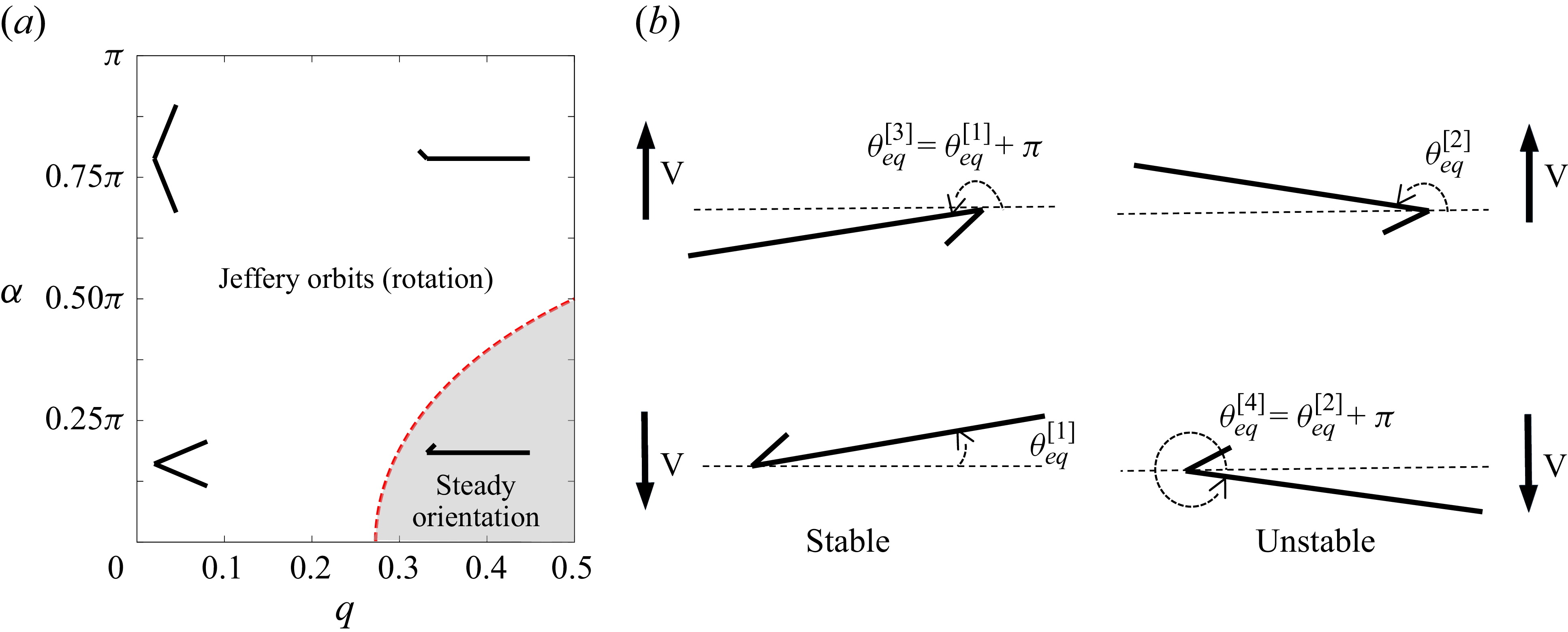
 (q,α)
 q
 α
 π

 r0(ζ)
 ζ
 (x1,x2)
 fs
 R0(ζ)
 rb(t)
 θ(t)
 x1
 R(ζ,t)
 fs

 θeq
 q=0.4
 α=0.230π
 I
 θeq[3]=θeq[1]+π=3.1792
 θeq[2]=3.0813
 I=0

 θeq
 q=0.4,α=0.180π
 I
 I=0
 I
 I=0
 θeq[3]=θeq[1]+π=3.1745,θeq[2]=3.0864

 θeq
 I
 q=0.4
 α
 α=0.180π
 α=0.230π
 I

 αmax
 I
 θeq
 α
 q
 I
 αmax(q,I)
 q,α
 I=0

 α
 (q,α)
 α
 q
 I
 θeq
 λ3
 α
 q=0.4
 I=0
 I=3,600

 θ(t)
 dY/dt
 I=0
 I=3600
 θ(t)
 2π
 α>αmax
 α=αmax
 α<αmax

 θ(t)
 I=0
 I=3600
 q=0.4
 α=0.667π>αmax
 Tperiod
 (α−αmax)
 I=0
 I=3600
 q=0.4
 Tperiod∼(α−αmax)−1/2
 π

 Y(t)
 I=0
 I=3600
 q=0.4
 α
 α<αmax
 α>αmax

 θeq
 I
 p=0.2, β=8
 I=0
 θeq[3]=1.7452
 θeq[2]=1.6724

 q=0.4,α=0.230π

 θeq
 I
 q=0.452
 α=0.125π
 I=0
 θeq[3]=θeq[1]+π=3.1540
 θeq[2]=3.1131

 θeq
 I
 α
 q=0.452
 α
 α


 Open access

