1. INTRODUCTION
The classical theory of statistical signal extraction presupposes lengthy data sequences, which are assumed, in theory, to be doubly infinite or semi-infinite (see, for example, Whittle, 1983). In many practical cases, and in most econometric applications, the available data are, to the contrary, both strongly trended and of a limited duration.
This paper is concerned with the theory of finite-sample signal extraction, and it shows how the classical Wiener–Kolmogorov theory of signal extraction can be adapted to cater to short sequences generated by processes that may be nonstationary.
Alternative methods of processing finite samples, which work in the frequency domain, are also described, and their relation to the time-domain implementations of the Wiener–Kolmogorov methods are demonstrated. The frequency-domain methods have the advantage that they are able to achieve clear separations of components that reside in adjacent frequency bands in a way that the time-domain methods cannot.
2. WIENER–KOLMOGOROV FILTERING OF SHORT STATIONARY SEQUENCES
In the classical theory, it is assumed that there is a doubly infinite sequence of observations, denoted, in this paper, by y(t) = {yt; t = 0,±1,±2,…}. Here, we shall assume that the observations run from t = 0 to t = T − 1. These are gathered in the vector y = [y0,y1,…, yT−1]′, which is decomposed as

where ξ is the signal component and η is the noise component. It may be assumed that the latter are from independent zero-mean Gaussian processes that are completely characterized by their first and second moments. Then,

A consequence of the independence of ξ and η is that D(y) = Ω = Ωξ + Ωη.
The autocovariance or dispersion matrices, which have a Toeplitz structure, may be obtained by replacing the argument z within the relevant autocovariance generating functions by the matrix

which is derived from the identity matrix IT = [e0,e1,…, eT−1] by deleting the leading column and appending a column of zeros to the end of the array. Using LT in place of z in the autocovariance generating function γ(z) of the data process gives

where FT = LT′ is in place of z−1. Because LT and FT are nilpotent of degree T, such that LTq,FTq = 0 when q ≥ T, the index of summation has an upper limit of T − 1.
The optimal predictors of the signal and the noise components are


which are their minimum-mean-square-error estimates.
The corresponding error dispersion matrices, from which confidence intervals for the estimated components may be derived, are


These formulas contain D{E(ξ|y)} = C(ξ,y)D−1(y)C(y,ξ) and D{E(η|y)} = C(η,y)D−1(y)C(y,η), which give the variability of the estimated components relative to their zero-valued unconditional expectations. The results follow from the ordinary algebra of conditional expectations, of which an account has been given by Pollock (1999). (Equations (5) and (6) are the basis of the analysis in Pollock, 2000.)
It can be seen from (5) and (6) that y = x + h. Therefore, only one of the components needs to be calculated. The estimate of the other component may be obtained by subtracting the calculated estimate from y. Also, the matrix inversion lemma indicates that

Therefore, (7) and (8) represent the same quantity, which is to be expected in view of the adding up.
The estimating equations can be obtained via the criterion

Because S(ξ,η) is the exponent of the normal joint density function N(ξ,η), the estimates of (5) and (6) may be described, alternatively, as the minimum chi-square estimates or as the maximum-likelihood estimates.
Setting η = y − ξ gives the function

The minimizing value is

where the second equality depends upon the first of the identities of (9).
A simple procedure for calculating the estimates x and h begins by solving the equation

for the value of b. Thereafter, one can generate

If Ωξ and Ωη correspond to the dispersion matrices of moving-average processes, then the solution to equation (13) may be found via a Cholesky factorization that sets Ωξ + Ωη = GG′, where G is a lower-triangular matrix with a limited number of nonzero bands. The system GG′b = y may be cast in the form of Gp = y and solved for p. Then, G′b = p can be solved for b. The procedure has been described by Pollock (2000).
3. FILTERING VIA FOURIER METHODS
A circular stochastic process of order T is one in which the autocovariance matrix of a random vector x = [x0,x1,…, xT−1]′, generated by the process, is unchanged when the elements of x are subjected to a cyclical permutation. Such a process is the finite equivalent of a stationary stochastic process.
The circular permutation of the elements of the sequence is effected by the matrix operator

which is formed from the identity matrix IT by moving the leading column to the back of the array. The powers of KT are T-periodic such that KTq+T = KTq. Moreover, any circular matrix of order T can be expressed as a linear combination of the basis matrices IT,KT,…, KTT−1.
The matrix KT has a spectral factorization that entails the discrete Fourier transform and its inverse. Let

denote the symmetric Fourier matrix, of which the generic element in the jth row and tth column is

The matrix U is unitary, which is to say that it fulfils the condition

where U = T−1/2[W−jt; t,j = 0,…,T − 1] denotes the conjugate matrix.
The circulant lag operator can be factorized as

where

is a diagonal matrix whose elements are the T roots of unity, which are found on the circumference of the unit circle in the complex plane. Observe also that D is T-periodic, such that Dq+T = Dq, and that Kq = UDqU = UDqU for any integer q. (An account of the algebra of circulant matrices has been provided by Pollock, 2002. See also Gray, 2002.)
The matrix of the circular autocovariances of the data is obtained by replacing the argument z in the autocovariance generating function γ(z) by the matrix KT:

The circular autocovariances would be obtained by wrapping the sequence of ordinary autocovariances around a circle of circumference T and adding the overlying values. Thus

Given that lim(τ → ∞)γτ = 0, it follows that γτ○ → γτ as T → ∞, which is to say that the circular autocovariances converge to the ordinary autocovariances as the circle expands.
The circulant autocovariance matrix is amenable to a spectral factorization of the form

wherein the jth element of the diagonal matrix γ(D) is

This represents the cosine Fourier transform of the sequence of the ordinary autocovariances, and it corresponds to an ordinate (scaled by 2π) sampled at the point ωj = 2πj/T, which is a Fourier frequency, from the spectral density function of the linear (i.e., noncircular) stationary stochastic process.
The method of Wiener–Kolmogorov filtering can also be implemented using the circulant dispersion matrices that are given by

wherein the diagonal matrices γξ(D) and γη(D) contain the ordinates of the spectral density functions of the component processes. By replacing the dispersion matrices within (5) and (6) by their circulant counterparts, we derive the following formulas:


Similar replacements within the formulas (7) and (8) provide the expressions for the error dispersion matrices that are appropriate to the circular filters.
The filtering formulas may be implemented in the following way. First, a Fourier transform is applied to the data vector y to give Uy, which resides in the frequency domain. Then, the elements of the transformed vector are multiplied by those of the diagonal weighting matrices Jξ = γξ(D){γξ(D) + γη(D)}−1 and Jη = γη(D){γξ(D) + γη(D)}−1. Finally, the products are carried back into the time domain by the inverse Fourier transform, which is represented by the matrix U. (An efficient implementation of a mixed-radix fast Fourier transform, which is designed to cope with samples of arbitrary sizes, has been provided by Pollock, 1999. The usual algorithms demand a sample size of T = 2n).
The frequency-domain realizations of the Wiener–Kolmogorov filters have sufficient flexibility to accommodate cases where the component processes ξ(t) and η(t) have band-limited spectra that are zero-valued beyond certain bounds. If the bands do not overlap, then it is possible to achieve a perfect decomposition of y(t) into its components.
Let Ωξ○ = UΛξU, Ωη○ = UΛηU, and Ω○ = U(Λξ + Λη)U, where Λξ and Λη contain the ordinates of the spectral density functions of ξ(t) and η(t), sampled at the Fourier frequencies. Then, if these spectra are disjoint, there will be ΛξΛη = 0, and the dispersion matrices of the two processes will be singular. The matrix Ωy○ = Ωξ○ + Ωη○ will also be singular, unless the domains of the spectral density functions of the component processes partition the frequency range. Putting these details into (26) gives

where {Λξ + Λη}+ denotes a generalized inverse. The corresponding error dispersion matrix is

But, if ΛξΛη = 0, then Λξ(Λξ + Λη)+Λξ = Λξ, and so the error dispersion is manifestly zero, which implies that x = ξ.
The significant differences between the time-domain and frequency-domain realizations of the Wiener–Kolmogorov filters occur at the ends of the sample. In the time-domain version, the coefficients of the filter vary as it moves through the sample, in a manner that prevents the filter from reaching beyond the bounds of the sample.
In the frequency-domain version, the implicit filter coefficients, which do not vary, are applied to the sample via a process of circular convolution. Thus, as it approaches the end of the sample, the filter takes an increasing proportion of its data from the beginning.
The implicit filter coefficients of the frequency-domain method are the circularly wrapped versions of the coefficients of a notional time-domain filter, defined in respect of y(t) = {yt; t = 0,±1,±2,…}, which may have an infinite impulse response. As the circle expands, the wrapped coefficients converge on the original coefficients in the same way as the circular autocovariances converge on the ordinary autocovariances.
Even when they form an infinite sequence, the coefficients of the notional time-domain filter will have a limited dispersion around their central value. Thus, as the sample size increases, the proportion of the filtered sequence that suffers from the end-effects diminishes, and the central values from the time-domain filtering, realized according to the formulas (5) and (6), and the frequency-domain filtering, realized according to (26) and (27), will converge point on point. By extrapolating the sample by a short distance at either end, one should be able to place the end-effects of the frequency-domain filter out of range of the sample.
Example
The frequency response of a circular filter applied to a finite sample of T data points is a periodic function defined over a set of T adjacent Fourier frequencies ωj = 2πj/T, where j takes T consecutive integer values. It is convenient to set j = 0,1,…,T − 1, in which case the response is defined over the frequency interval [0,2π).
However, it may be necessary to define the response over the interval [−π,π), which is used, conventionally, for representing the continuous response function of a filter applied to a doubly infinite data sequence. In that case, j = 0,±1,…, [T/2], where [T/2] is the integral part of T/2.
The responses at the T Fourier frequencies can take any finite real values, subject only to the condition that λj = λT−j or to the equivalent condition that λj = λ−j. These restrictions will ensure that the corresponding filter coefficients form a real-valued symmetric sequence. The T coefficients of the circular filter may be obtained by applying the inverse discrete Fourier transform to the responses.
It is convenient, nevertheless, to specify the frequency response of a circular filter by sampling a predefined continuous response. Then, the coefficients of the circular filter are formally equivalent to those that would be found by wrapping the coefficients of an ordinary filter, pertaining to the continuous response, around a circle of circumference T and adding the coincident values.
A filter that has a band-limited frequency response has an infinite set of filter coefficients. In that case, it is not practical to find coefficients of the circular filter by wrapping the coefficients of the ordinary filter. Instead, they must be found by transforming a set of frequency-domain ordinates.
A leading example of a band-limited response is provided by an ideal lowpass frequency-selective filter that has a boxcar frequency response. Two versions of the filter may be defined, depending on whether the transitions between pass band and stop band occur at Fourier frequencies or between Fourier frequencies.
Consider a set of T frequency-domain ordinates sampled, over the interval [−π,π), from a boxcar function, centered on ω0 = 0. If the cutoff points lie between ±ωd = ±2πd/T and the succeeding Fourier frequencies, then the sampled ordinates will be

The corresponding filter coefficients will be given by

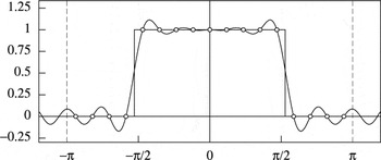
where ω1 = 2π/T. This function is just an instance of the Dirichlet kernel—see, for example, Pollock (1999). Figure 1 depicts the frequency response for this filter at the Fourier frequencies, where λj = 0,1. It also depicts the continuous frequency response that would be the consequence of applying an ordinary filter with these coefficients to a doubly infinite data sequence.

The frequency response of the 17-point wrapped filter defined over the interval [−π,π). The values at the Fourier frequencies are marked by circles.
It is notable that a casual inspection of the continuous response would lead one to infer the danger of substantial leakage, whereby elements that lie within the stop band are allowed to pass into the filtered sequence. In fact, with regard to the finite sample, there is no leakage.
If the cutoff points fall on the Fourier frequencies ±ωd, and if λd = λ−d = ½, then the filter coefficients will be

4. POLYNOMIALS AND THE MATRIX DIFFERENCE OPERATOR
The remaining sections of this paper are devoted to methods of filtering nonstationary sequences generated by linear stochastic processes with unit roots in an autoregressive operator. To support the analysis, the present section deals with the algebra of the difference operator and of the summation operator, which is its inverse. When it is used to cumulate data, the summation operator automatically generates polynomial functions of the discrete-time index. This feature is also analyzed.
The matrix that takes the pth difference of a vector of order T is

We may partition this matrix so that ∇Tp = [Q*,Q]′, where Q*′ has p rows. If y is a vector of T elements, then

and g* is liable to be discarded, whereas g will be regarded as the vector of the pth differences of the data.
The inverse matrix is partitioned conformably to give ∇T−p = [S*,S]. It follows that

and that

If g* is available, then y can be recovered from g via

The lower-triangular Toeplitz matrix ∇T−p = [S*,S] is completely characterized by its leading column. The elements of that column are the ordinates of a polynomial of degree p − 1, of which the argument is the row index t = 0,1,…,T − 1. Moreover, the leading p columns of the matrix ∇T−p, which constitute the submatrix S*, provide a basis for all polynomials of degree p − 1 that are defined on the integer points t = 0,1,…,T − 1.
It follows that S* g* = S*Q*′y contains the ordinates of a polynomial of degree p − 1, which is interpolated through the first p elements of y, indexed by t = 0,1,…, p − 1, and which is extrapolated over the remaining integers t = p,p + 1,…,T − 1.
A polynomial that is designed to fit the data should take account of all of the observations in y. Imagine, therefore, that y = φ + η, where φ contains the ordinates of a polynomial of degree p − 1 and η is a disturbance term with E(η) = 0 and D(η) = Ωη. Then, in forming an estimate f = S* r* of φ, we should minimize the sum of squares η′Ωη−1η. Because the polynomial is fully determined by the elements of a starting-value vector r*, this is a matter of minimizing

with respect to r*. The resulting values are

An alternative representation of the estimated polynomial is available, which avoids the inversion of Ωη. This is provided by the identity

which gives two representations of the projection matrix P*. The equality follows from the fact that, if Rank[R,S*] = T and if S*′Ωη−1R = 0, then

Setting R = ΩηQ gives the result.
Grenander and Rosenblatt (1957) have shown that, when the disturbances are generated by a stationary stochastic process, the generalized least-squares (GLS) estimator of a polynomial regression that incorporates the matrix Ωη is asymptotically equivalent to the ordinary least-squares (OLS) estimator that has the identity matrix IT in place of Ωη. The result has also been demonstrated by Anderson (1971). It means that one can use the OLS estimator without significant detriment to the quality of the estimates.
The result is proved by showing that the metric of the GLS regression is asymptotically equivalent to the Euclidean metric of OLS regression. It is required that, in the limit, the columns of Ωη−1S* and S* should span the same space. It follows that the projection operator P* of (40) is asymptotically equivalent to S*(S*′S*)−1S*′ = I − Q(Q′Q)−1Q′.
The residuals of an OLS polynomial regression of degree p, which are given by y − f = Q(Q′Q)−1Q′y, contain the same information as the vector g = Q′y of the pth differences of the data. The difference operator has the effect of nullifying the element of zero frequency and of attenuating radically the adjacent low-frequency elements. Therefore, the low-frequency spectral structures of the data are not perceptible in the periodogram of the differenced sequence.
On the other hand, the periodogram of a trended sequence is liable to be dominated by its low-frequency components, which will mask the other spectral structures. However, the periodogram of the polynomial regression residuals can be relied upon to reveal the spectral structures at all frequencies. Moreover, by varying the degree p of the polynomial, one is able to alter the relative emphasis that is given to high-frequency and low-frequency structures.
5. WIENER–KOLMOGOROV FILTERING OF NONSTATIONARY DATA
The treatment of trended data must accommodate stochastic processes with drift. Therefore, it will be assumed that, within y = ξ + η, the trend component ξ = φ + ζ is the sum of a vector φ, containing ordinates sampled from a polynomial in t of degree p at most, and a vector ζ from a stochastic process with p unit roots that is driven by a zero-mean process.
If Q′ is the pth difference operator, then Q′φ = μι, with ι = [1,1,…,1]′, will contain a constant sequence of values, which will be zeros if the degree of the stochastic drift is less than p, which is the degree of differencing. Also, Q′ζ will be a vector sampled from a mean-zero stationary process. Therefore, δ = Q′ξ is from a stationary process with a constant mean. Thus, there is

where

Let the estimates of ξ, η, δ = Q′ξ and κ = Q′η be denoted by x, h, d, and k, respectively. Then, with E(g) = E(δ) = μι, there is


and these vectors obey an adding-up condition:

In (44), the low-pass filter matrix Zδ = Ωδ(Ωδ + Q′ΩηQ)−1 will virtually conserve the vector μι, which is an element of zero frequency. In (45), the complementary high-pass filter matrix Zκ = Q′ΩηQ(Ωδ + Q′ΩηQ)−1 will virtually nullify the vector. Its failure to do so completely is attributable to the fact that the filter matrix is of full rank. As the matrix converges on its asymptotic form, the nullification will become complete. It follows that, even when the degree of the stochastic drift is p, one can set


The estimates of ξ and η may be obtained by integrating, or reinflating, the components of the differenced data to give

For this, the starting values d* and h* are required. The initial conditions in d* should be chosen so as to ensure that the estimated trend is aligned as closely as possible with the data. The criterion is

The solution for the starting values is

The starting values of k* are obtained by minimizing the (generalized) sum of squares of the fluctuations:

The solution is

It is straightforward to show that, when (42) holds,

which is to say that the addition of the estimates produces the original data series. As in (40), let P* = S*(S*′Ωη−1S*)−1S*′Ωη−1. Then, the two components can be written as


Adding these, using d + k = Q′y from (46), gives

Here, the first equality follows from the fact that (I − P*)S* = 0, and the second follows from the identity SQ′ + S*Q*′ = I, which is from (35). In view of (49), it can be seen that the condition x + h = y signifies that the criteria of (50) and (52) are equivalent.
The starting values k* and d* can be eliminated from the expressions for x and h, which provide the estimates of the components. Substituting the expression for PQ from (40) into h = (I − P*)Sk = PQ Sk together with the expression for k from (48) and using the identity Q′S = IT gives

A similar reduction can be pursued in respect to the equation x = (I − P*)Sd + P* y = PQ Sd + (I − PQ)y. However, it follows immediately from (54) that

Observe that the filter matrix Zη = ΩηQ(Ωδ + Q′ΩηQ)−1 of (58), which delivers h = Zη g, differs from the matrix Zκ = Q′Zη of (48), which delivers k = Zκ g, only in respect to the matrix difference operator Q′. The effect of omitting the operator is to remove the need for reinflating the filtered components and thus to remove the need for the starting values.
Equation (59) can also be derived via a straightforward generalization of the chi-square criterion of (10). If we regard the elements of δ* as fixed values, then the dispersion matrix of ξ = S*δ* + Sδ is the singular matrix D(ξ) = Ωξ = SΩδ S′. On setting η = y − ξ in (10) and replacing the inverse of Ωξ−1 by the generalized inverse Ωξ+ = QΩδ−1Q′, we get the function

of which the minimizing value is

The matrix inversion lemma gives

and putting this into (61) gives the expression of (59). The matrix of (62) also constitutes the error dispersion matrix D(η|y) = D(ξ|y), which, in view of their adding-up property (54), is common to the estimates of the two components.
It is straightforward to compute h when Ωη and Ωδ have narrow-band moving-average forms. Consider h = ΩηQb, where b = (Q′ΩηQ + Ωδ)−1g. First, b may be calculated by solving the equation (Q′ΩηQ + Ωδ)b = g. This involves the Cholesky decomposition of Q′ΩηQ + Ωδ = GG′, where G is a lower-triangular matrix with a number of nonzero diagonal bands equal to the recursive order of the filter. The system GG′b = Gp = g is solved for p. Then, G′b = p is solved for b. These are the recursive operations. Given b, then h can be obtained via direct multiplications.
6. APPLYING THE FOURIER METHOD TO NONSTATIONARY SEQUENCES
The method of processing nonstationary sequences that has been expounded in the preceding section depends upon the finite-sample versions of the difference operator and the summation operator. These are derived by replacing z in the functions ∇(z) = 1 − z and Σ(z) = (1 − z)−1 = {1 + z + z2 + ···} by the finite-sample lag operator LT, which gives rise to a nonsingular matrix ∇(LT) = [Q*,Q]′ and its inverse ∇−1(LT) = Σ(LT) = [S*,S].
The identity of (40), which is due to the interaction of the matrices S* and Q′, has enabled us to reinflate the components of the differenced sequence Q′y = g = d + k without explicitly representing the initial conditions or start-values d* and k* that are to be found in equations (55) and (56).
The operators that are derived by replacing z in ∇(z) and Σ(z) by the circulant lag operator KT are problematic. On the one hand, putting KT in place of z within ∇(z) results in a noninvertible matrix of rank T − 1. On the other hand, the replacement of z within the series expansion of Σ(z) results in a nonconvergent series that corresponds to a matrix in which all of the elements are uniformly of infinite value.
In applying the Fourier method of signal extraction to nonstationary sequences, one recourse is to use ∇(LT) and Σ(LT) for the purposes of reducing the data to stationarity and for reinflating them. The components δ and κ of the differenced data may estimated via the equations


For a vector μι of repeated elements, there will be Pδ μι = μι and Pκ μι = 0.
Whereas the estimates of δ, κ may be extracted from g = Q′y by the Fourier method, the corresponding estimates x, h of ξ, η will be found from equations (55) and (56), which originate in the time-domain approach and which require explicit initial conditions.
It may also be appropriate, in this context, to replace the criteria of (50) and (52), which generate the values of d* and k*, by simplified criteria wherein Ωη is replaced by the identity matrix IT. Then

The available formulas for the summation of sequences provide convenient expressions for the values of the elements of S*′S* (see, e.g., Banerjee, Dolado, Galbraith, and Hendry, 1993, p. 20).
An alternative recourse, which is available in the case of a high-pass or bandpass filter that nullifies the low-frequency components of the data, entails removing the implicit differencing operator from the filter. (In an appendix to their paper, Baxter and King, 1999, demonstrate the presence, within a symmetric bandpass filter, of two unit roots, i.e., of a twofold differencing operator.)
Consider a filter defined in respect to a doubly infinite sequence and let φ(z) be the transfer function of the filter, that is, the z-transform of the filter coefficients. Imagine that φ(z) contains the factor (1 − z)p and let ψ(z) = (1 − z)−pφ(z). Then, ψ(z) defines a filter of which the finite-sample version can be realized by the replacement of z by KT.
Because KT = UDU, the filter matrix can be factorized as ψ(KT) = Ψ = Uψ(KT)U. On defining Jψ = ψ(KT), which is a diagonal weighting matrix, the estimate of the signal component is given by the equation

Whichever procedure is adopted, the Fourier method is applied to data that have been reduced to stationarity by differencing. Given the circularity of the method, it follows that as a filter approaches one end of the sample it will take an increasing proportion of its data from the other end. To avoid some of the effects of this, one may extrapolate the data at both ends of sample. The extrapolation can be done either before or after the data have been differenced. After the filtering, the extra-sample elements may be discarded.
If the trended data have been extrapolated, then the starting values d* and k*, which are required by the first procedure, may be obtained by minimizing the quadratic functions (50) and (52) defined over the enlarged data set. Otherwise, if the differenced data have been extrapolated, then the extra-sample points of the filtered sequence are discarded prior to its reinflation, and the quadratic functions that are to be minimized in pursuit of the starting values are defined over T points corresponding to the original sample.
Extrapolating the differenced data has the advantage of facilitating the process of tapering, whereby the ends of the sample are reduced to a level at which they can meet when the data are wrapped around a circle. The purpose of this is to avoid any radical disjunctions that might otherwise occur at the meeting point and that might have ill effects throughout the filtered sequences.
We should also note that, in the case of a finite bandpass filter, a third possibility arises. This is to apply the filter directly to the original, undifferenced, data. Such a procedure has been followed both by Baxter and King (1999) and by Christiano and Fitzgerald (2003). The latter have found an ingenious way of extrapolating the data so as to enable the filter to generate values at the ends of the sample.
The Fourier method can be used to advantage whenever the components of the data are to be found in disjoint frequency intervals. If the components are separated by wide spectral dead spaces, then it should be possible to extract them from the data with filters that have gradual transitions that are confined to the dead spaces. In that case, Wiener–Kolmogorov time-domain filters of low orders can be used. However, when the components are adjacent or are separated by narrow dead spaces, it is difficult to devise a time-domain filter with a transition that is sharp enough and that does not suffer from problems of instability. Then, a Fourier method should be used instead.
Example
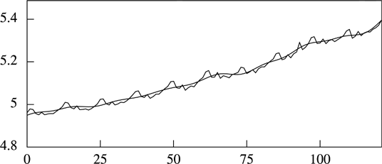
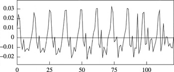
Figure 2 show the logarithms of a monthly sequence of 132 observations of the U.S. money supply, through which a trend has been interpolated, and Figure 3 shows the sequence of the deviations from the tend. The data are from Bolch and Huang (1974).

The plot of the logarithms of 132 monthly observations on the U.S. money supply, beginning in January 1960. A trend, estimated by the Fourier method, has been interpolated through the data.

The deviations of the logarithmic money-supply data from the interpolated trend.
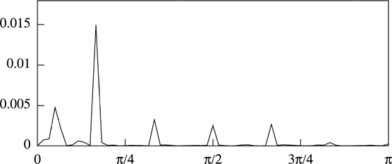
The trend has been estimated with reference to Figure 4, which shows the periodogram of the residuals from a quadratic detrending of the data. There is a tall spike in the periodogram at ω11 = π/6, which represents the fundamental frequency of an annual seasonal fluctuation. To the left of this spike, there is a spectral mass, which belongs to the trend component. Its presence is an indication of the inadequacy of the quadratic detrending. To remove this spectral mass and to estimate the trend more effectively, a Fourier method has been deployed.

The periodogram of the residuals from the quadratic detrending of the logarithmic money-supply data.
An inspection of the numerical values of the ordinates of the periodogram has indicated that, within the accuracy of the calculations, the element at ω10, which is adjacent to the seasonal frequency, is zero-valued. This defines the point of transition of the low-pass filter that has been used to isolate the trend component of the data. A filter with a less abrupt transition would allow the powerful seasonal component to leak into the trend and vice versa. Experiments using Wiener–Kolmogorov time-domain filters have shown the detriment of this.
The trend in Figure 2 has been created by reinflating a sequence that has been synthesized from the relevant ordinates selected from the Fourier transform of the twice differenced data. The latter have a positive mean value, which corresponds to a quadratic drift in the original data. The differenced data have not been extrapolated, because there appears to be no detriment in the end-effects. Moreover, the regularity of the seasonal fluctuations, as revealed by the sequence of the deviations from the trend in Figure 3, is a testimony to the success in estimating the trend.