I. Introduction
Faced with an enormous number of choices of different wines, consumers often rely on expert opinion to guide their purchase decision. Having recognized the influence on their sales and profits of winning awards, wineries actively participate in different wine competitions. Evaluation of wine quality in wine competitions is usually conducted by professional wine judges. Wine quality is an abstract measure that is difficult to define. In addition, a judge's personal perception of a wine's quality may be affected by extraneous factors, such as the order in which the wines are tasted and the other wines in the lineup. A substantial lack of consensus has been found among wine judges (Cao and Stokes, Reference Cao and Stokes2010; Gawel and Godden, Reference Gawel and Godden2008; Hodgson, Reference Hodgson2008, Reference Hodgson2009). As a consequence, the lack of consistency may compromise the credibility of wine competitions, which could lead to a loss of consumer confidence in the competition results.
Consensus, or interrater agreement, refers to the degree of agreement among judges. Most of wine-tasting scores are ordinal. Some of the commonly used statistics to measure agreement for ordinal data are: Spearman's rank correlation, Cohen's kappa (Cohen, Reference Cohen1960), and Fleiss's kappa (Fleiss, Reference Fleiss1971). Spearman's rank correlation measures the correlation between the ranks of two variables. Cohen's kappa is a chance-corrected measure of interrater agreement for qualitative data (categorical, ordinal, etc.). Note that Cohen's kappa measures agreement only between two raters. Fleiss's kappa is a generalization of Cohen's kappa to measure agreement among K (K>2) raters. All these measures have a range from –1 to 1, where the sign indicates the direction and the magnitude indicates the strength of agreement. The closer the statistics are to 1, the stronger the positive interrater agreement.
Ashton (Reference Ashton2012) reviewed a number of earlier studies and concluded that consensus of wine judges is considerably below the consensus of judges in other fields, but wine ratings appear not to be entirely random. The study used the Pearson correlation (r=0.34) to measure the average level of consensus across the wines between the ratings of each pair of judges. Although this correlation provides some information on the consensus of wine judges, it does not directly quantify randomness versus consensus in wine quality ratings. In fact, all the above mentioned statistics fail to quantify randomness versus consensus regarding interrater agreement. To address this issue, this study will investigate (1) whether wine ratings consist of a mixture of two components (i.e., randomness and consensus); (2) the proportions in the mixture of the two components; and (3) whether the corresponding mixed model can adequately explain the variation in wine ratings.
In this paper, a permutation-based mixed model is proposed to quantify randomness versus consensus in wine ratings. Specifically, the distribution of observed average wine ratings is modeled as a mixture of the distribution of average wine ratings under complete randomness generated based on a permutation method and the distribution of average wine ratings under perfect consensus, which can be easily obtained by sorting the wine ratings for each judge. This study shows that such a model can provide an excellent model fit and a direct measure to quantify randomness versus consensus in wine ratings. The method is demonstrated with data analysis from a major wine competition and a simulation study.
II. Examination of Wine-Tasting Data
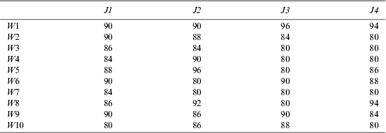
The analysis is conducted using data from the 2009 California State Fair Commercial Wine Competition (CSFCWC). A total of 68 judges were assigned to 17 panels to evaluate 2,496 different wines. Each panel of 4 judges evaluated around 150 different wines over two days. The judges, who each served on a single panel, were instructed to provide ordinal grades (i.e., No award, Bronze, Bronze+), which were later transformed to numerical scores (i.e., 80, 84, 86, 88, 90, 92, 94, 96). In each panel, the ranking of the wines is determined by the average scores (ratings) across the judges. Table 1 shows a sample of the observed ratings from one of the panels (denoted as Panel A), where the rows represent the wines, and the columns represent the judges.
A Subset of Raw Data from Panel A
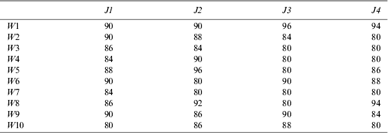
To make the examination of the wine ratings more straightforward, a color plot (or heat map) is constructed to display the data (see Figure 1). A warmer color corresponds to a higher rating. Specifically, the colors brown, red, orange, yellow, green, light blue, blue, and dark blue correspond to ratings of, respectively, 96, 94, 92, 90, 88, 86, 84, 80. The left-hand panel in Figure 1 displays a subset of the observed ratings in Panel A. From left to right, the columns represent the ratings assigned by the four judges. From top to bottom, the rows correspond to the wines included in the panel. The center panel in Figure 1 shows the ratings under perfect consensus for the same group of judges (denoted as the consensus set of ratings). It is constructed by sorting the ratings from highest to lowest for each judge. It represents the case in which judges are in perfect agreement on the order of the wines, and they are allowed to use different ratings. For example, the top-ranking wine was assigned 92, 96, 96, and 94 by the four judges, respectively. The right-hand panel shows the ratings under complete randomness (denoted as the random set of ratings). It is constructed by permuting (shuffling) the ratings for each judge, which mimics the case in which each judge randomly assigns ratings to the wines, and the ratings are randomly picked from the values used in his rating pattern.
Wine-Tasting Data Heat Map

The wine ratings shown in Figure 1 have several interesting features. First, the judges have different rating patterns (profiles), which can be seen from the center panel of ratings in the consensus set. In terms of bias, which is the systematic difference between a judge's rating and the average rating from all the judges, Judge J4 is more stringent than Judge J1 because J4 assigned more lower ratings to the wines than did J1. In terms of discrimination, which measures a judge's ability to distinguish wines based on their quality (Cao and Stokes, Reference Cao and Stokes2010), Judge J2 used a wider range of ratings (with all eight levels) than Judge J1, who only used five levels. If the judges had the same rating pattern, the center panel would look like a layer cake, with the same number of different levels of ratings among judges. This first feature implicitly explains why the random ratings cannot be generated by assuming that each possible rating is equally likely to be assigned by a judge. Instead, by permuting the ratings for each judge, the respective rating pattern is maintained when simulating random ratings for each judge. In this paper, the statistical software R is used to produce permutation, where the probabilities for random selection are applied sequentially—that is, the probability of choosing the next item is the same among the remaining items. Such permutation methods have been commonly used in statistics to generate data under randomness, for example, in microarray data analysis (Cui et al., Reference Cui, Hwang, Qiu, Blades and Churchill2005; Tusher et al., Reference Tusher, Tibshirani and Chu2001).
Based on Figure 1, it appears that the observed ratings contain considerable amount of randomness. However, a certain degree of consensus is evident in the left-hand panel (observed ratings), compared to no consensus in the right-hand panel (random ratings). For example, there are six rows (i.e., wines) with the same rating from at least three judges in the left-hand panel, while in the right-hand panel there are only two rows with the same rating from three judges. The goal is to quantify randomness versus consensus among all the judges—that is, how much variation in observed ratings is from randomness and how much is from consensus.
III. Method
In statistics, a mixed distribution is used to describe the behavior of a random variable whose values are derived from an underlying set of other random variables. The history of data analysis using mixed models dates back more than 100 years to the famous statistician Karl Pearson (Reference Pearson1894); he fitted a mixture of two normal probability density functions with different means and variances. In his paper, Pearson suggested that the asymmetry in the distribution of the observed data (measurements on the ratio of forehead to body length of 1,000 crabs sampled from the Bay of Naples) stems from a mixture of two homogeneous subsets (i.e., two subspecies of crabs). More formally, a distribution f is a mixture of K component distributions f 1, f 2, …, f 3 if
 $$f\,(x) = \sum {_{k = 1}^K} \lambda _k f_k (x),$$
where the λ k are the mixing weights, λ k>0, and  $\sum {_{k = 1}^K} \lambda _k = 1$.
In the past 30 years, considerable advances (in theory and application) have been made in mixed models thanks to the advent of the modern computing techniques. Mixed models have been successfully applied in such fields as astronomy, biology, genetics, medicine, economics, and engineering, among many other research areas in the biological, physical, and social sciences (McLachlan and Peel, Reference McLachlan and Peel2000). In this paper, we use a mixed model to study the two components in wine ratings: randomness and consensus.
Wine competitions usually use the average ratings across judges to determine the ranking of wines. Let X be the average rating, which is a random variable, and d o(X) the density function of X under observation, d c(X) the density function of X under perfect consensus, and d r(X) the density function of X under complete randomness. Then the proposed model to describe the mixture distribution has the form of
 $$d_o (X) = p_r d_r (X) + (1 - p_r )d_c (X),$$
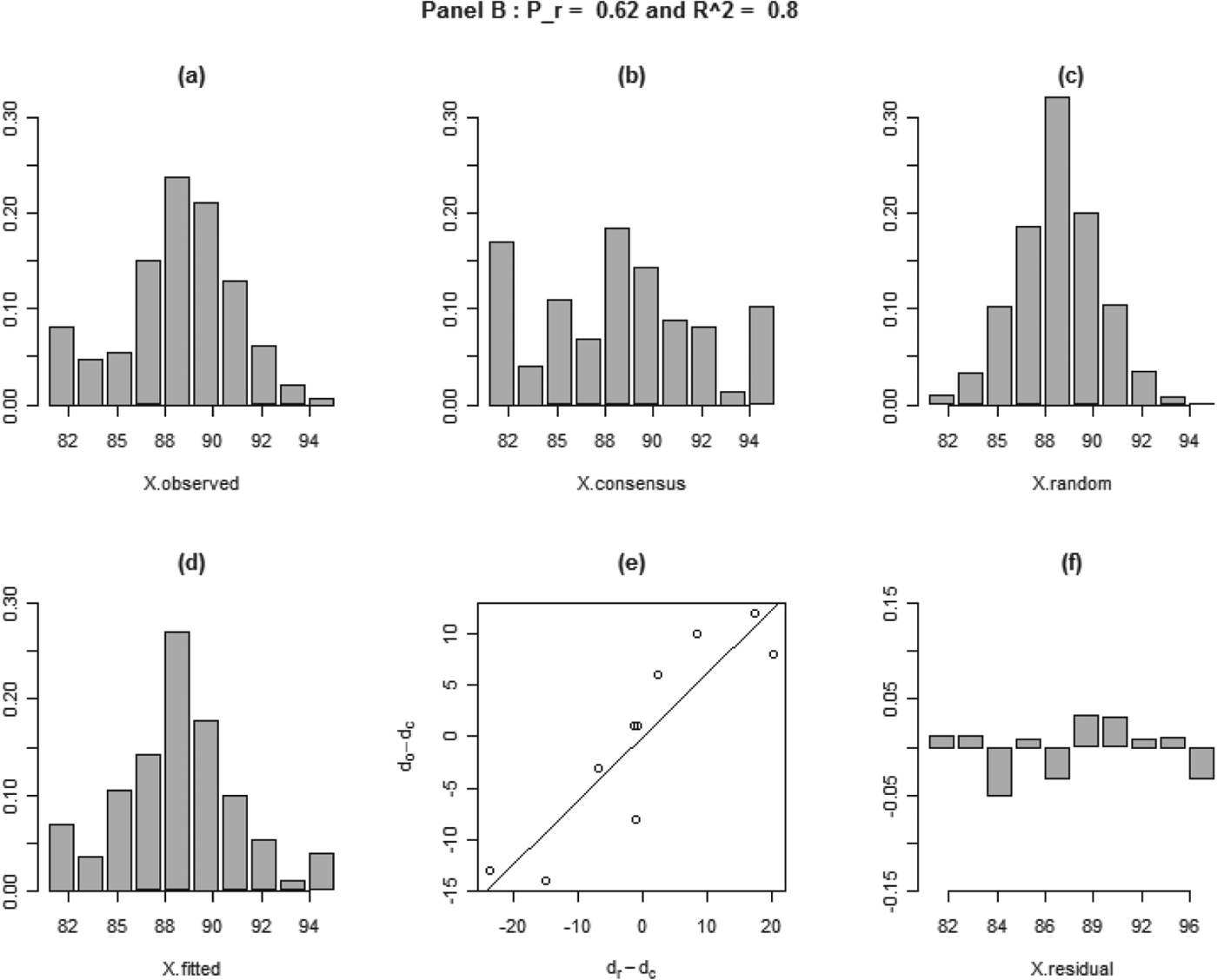
where p r is the proportion of the random component in the mixed model and 1 – p r is the proportion of the consensus component. An empirical estimate of the three densities can be conveniently obtained by constructing the density histogram. Plots (a), (b), and (c) in Figure 2, which is based on the data from a panel (denoted as Panel B) in the CSFCWC, are the histograms for the observed average ratings (X.observed in the original dataset), average ratings under perfect consensus (X.consensus in the consensus set), and average ratings under complete randomness (X.random in the random set), respectively. The range of the variables is partitioned into a fixed number of bins, in this case 10 bins. The empirical estimate of density is then the height of each bin (i.e., the relative frequency). One technical aspect is that 100 sets of the ratings under randomness (each set has the same number of wines as in the observed dataset) are generated to construct d r(X) from one set of random ratings, which results in quite unstable d r(X). Based on the application and simulation studies in the following, d r(X) becomes very stable with 100 permutation sets, and thus 100 sets is chosen for use in this method. Note that 100 permutation sets are used to construct a stable distribution of ratings under randomness, but this does not affect the number of bins chosen to estimate density d r(X). Increasing the number of permutation sets means increasing the data size, which does not change the density curve. The number of bins can be any fixed number—that is, 5, 10, or 20. In this study, 10 bins are used because it is a convenient number and it is sufficient to fit the model.
Plots for Panel B
Model (1) can be rewritten as
 $$d_o (X) - d_c (X) = p_r \left( {d_r (X) - d_c (X)} \right),$$
which is a zero-intercept simple linear regression model with d o(X) − dc(X) as the response variable and d r(X) − dc(X) as the explanatory variable. The regression coefficient p r can be easily computed using least squares estimation.
The proposed method is based on the average score for ordinal data. It should be noted that the quantification of randomness versus consensus is not measured directly by the average score as numerical values but modeled based on the distribution of the average score. The proposed method is also different from the ANOVA model based on the original data, where the factor for the judges measures the judges’ bias (stringent, neutral, or generous), the factor for wine measures the order of wines based on the general opinion of judges, and the error term accounts for the remaining unexplained variation. Note that the error term in the ANOVA model is not the same randomness studied in this paper. The randomness in Model (1) refers to the case in which each judge randomly assigns ratings to the wines, which do not depend on any parametric assumptions. The error term in the ANOVA model depends on the fitted model, which measures the unexplained variation after including the judge factor and the wine factor in the model.
IV. Application
Model (1) is applied to each of the 17 panels in the CSFCWC dataset. The probability of randomness p r varies from 0.62 to 0.85. Based on the scatter plot and the residual plot (see Figure 2 and Figure 3), Model (1) can capture the main pattern in the data. The coefficient of determination (R 2), which is the proportion of the total variation of outcomes explained by the model, varies from 0.80 to 0.95, indicating good to excellent model fit.
Figure 2 shows the results from Panel B, which has the lowest p r (p r=0.62) among all the panels. It means that there is 62% of randomness and 38% of consensus in those wine ratings. Plots (d), (e), and (f) are the histogram for the fitted average ratings (X.fitted) based on Model (1), the scatter plot of the response variable (d o(X) − dc(X)) and the explanatory variable (d r(X) − dc(X)) in the model, and the residual plot (X.fitted—X.observed). In addition to the evidence of R 2=0.8, the model fit can be assessed by (1) comparing plots (d) and (a) (the histogram of X.fitted versus the histogram of X.observed), which appear to have a similar shape; and (2) examining plots (e) and (f), which show that the fitted straight line has captured the linear relationship in the scatter plot and the residuals are well behaved (i.e., no outlier and no evidence of nonrandom pattern).
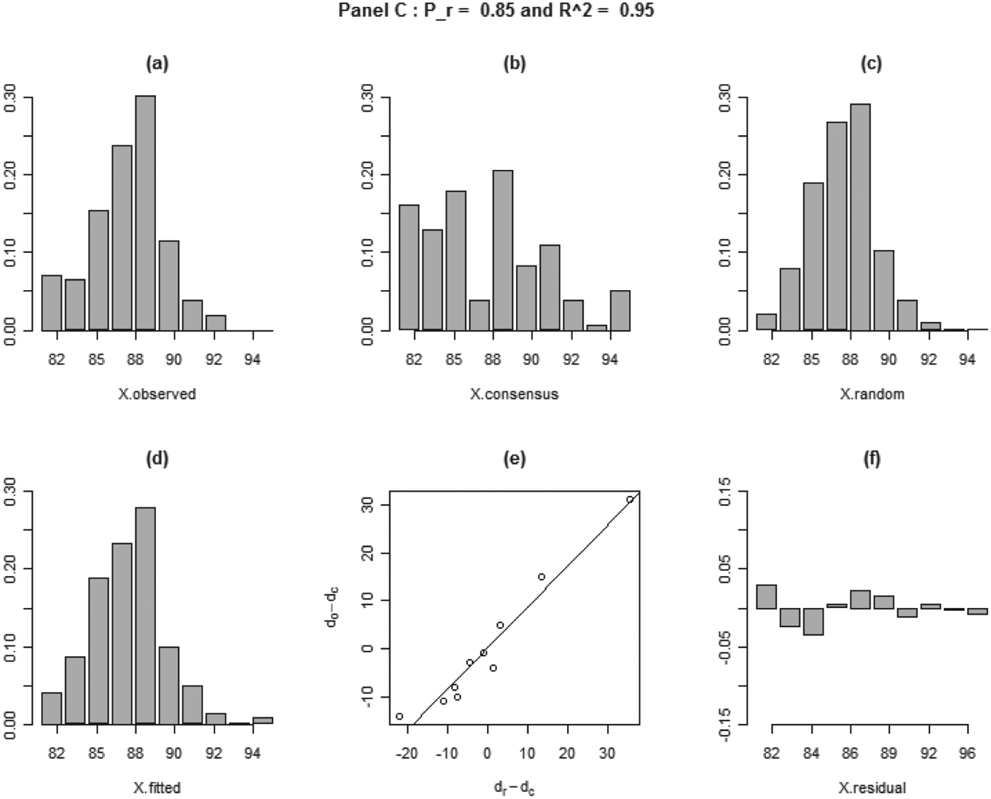
Figure 3 shows the results for the panel (denoted as Panel C), which has the highest p r (p r=0.85) among all the panels. It means that there is 85% of randomness and 15% of consensus in those wine ratings. The adequacy of model fit can be confirmed by R 2=0.95 and by examining the plots in Figure 3 in the same way as described for Figure 2.
Plots for Panel C
In all the panels considered, there is more randomness than consensus in wine ratings, which is indicated by p r > 0.5. In addition, the lowest p r and the highest p r among all the panels differ by more than 20%. This conclusion is supported by the adequate model fit of the data. It can also be corroborated through visual analytics. First, for all the panels, the histogram of X.observed resembles more closely the histogram of X.random than that of X.concensus, resulting in p r > 0.5. Second, for a panel with a smaller p r the histogram of X.observed has clearer influence than that of X.concensus and more obvious deviation from that of X.random. Note that the distribution of X.concensus generally is flatter than that of X.random because under consensus judges agree on the ranking of wines, which produces more extreme scores on two ends than does the random case. In Panel B, the distribution of X.observed is less spiked and has significantly more average ratings at the low end than does X.random (see the first two bins in the histogram), which can be attributed to a higher percentage of the consensus component in the mixed distribution. By comparison, in Panel C, the distribution of X.observed is almost a duplicate of the distribution of X.random, except for a few more average ratings at the low end. This indicates that the random component is the absolute dominant component in the mixed distribution and the consensus component becomes trivial. The visual comparison is consistent with the difference in the model-based p r in the two panels.
V. Simulation Study
In this section, we further investigate the performance of the proposed method by conducting a simulation study to examine whether the model can correctly quantify randomness versus consensus. With the simulation truth known, this study provides additional evidence regarding the utility of the method.
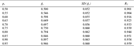
The study includes a spectrum of proportions of randomness (p r), which is set from 0.5 to 0.95 with an increment of 0.05. Based on the setup of the CSFCWC dataset, the generated wine ratings in each panel consist of a specific proportion (p r) of ratings, which are randomly selected (i.e., simple random selection in which each rating has the same probability of being chosen) from the random set, and the remaining proportion (1 − p r) of ratings, which are randomly selected from the consensus set. This produces a dataset with a mixture of p r of randomness and 1 − p r of consensus. Data are generated following this design for each panel, and the simulation is repeated 100 times.
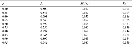
Table 2 summarizes the simulation results. The four columns in the tables represent the true value of p r, the estimate of p r (i.e.,  $\hat p_r $) and the standard deviation of the estimate (i.e.,
 $SD(\hat p_r )$) over the panels and 100 simulations, and R 2 to measure the model fit, respectively. The study shows that
 $\hat p_r $ is unbiased for the whole spectrum of p r, the variation of
 $\hat p_r $ is stable, and the fit of Model (1) is excellent, as indicated by an average R 2>0.9 for all the cases.
Simulation Results
VI. Discussion
In this paper, a permutation-based mixed model is proposed to quantify randomness versus consensus in wine quality ratings. Compared to the existing measures on interrater agreement, the new method has a number of advantages. First, it is simple to implement and easy to interpret. Many of the current statistics on interrater agreement provide a measure on the strength of consensus, but they do not directly measure the amount of randomness versus consensus in multirater studies. Unlike those measures, the proposed two-component mixed model provides a direct answer on the percentage of randomness (and consensus) in wine ratings.
Second, the method is flexible to allow wine judges to have their personal rating patterns. Note that there are different operational definitions of rater agreement. The two commonly used ones are (1) raters agree with one another on the exact ratings to be awarded, and (2) raters agree on which performance is better and which is worse. They respectively correspond to two types of behavior: (1) raters behave like “rating machines” (e.g., a computer program to rate essays), and (2) raters behave like independent witnesses who may have their own standard for evaluation. The wine quality ratings shown in Figure 1 clearly demonstrate that wine judges have independent rating patterns, so it is thus reasonable to follow the second definition of rater agreement. Note that Cohen's kappa and Fleiss's kappa measure rater agreement based on an exact matching of ratings (i.e., definition 1 of rater agreement). Spearman's rank correlation is an appropriate measure regarding definition 2 of rater agreement; however, it works for only two raters. The proposed method maintains judges’ own rating patterns (i.e., definition 2 of rater agreement), and it allows multiple judges in the study (i.e., judges can number more than two).
Third, the validity of the proposed method can be assessed by examining model fit of the mixture model. Many of the current rater-agreement statistics do not consider the quantitative composition of observed ratings. They are often used to test whether or not consensus is zero. Note that whether or not consensus is zero is generally not as relevant as how much consensus is in the ratings. By comparison, model diagnostics for simple linear regression models can be used to find out whether the proposed two-component mixed model provides adequate fit for the data and whether the quantification of randomness versus consensus for wine quality ratings is trustworthy. The adequate model fit from the real data analysis indicates strong evidence that wine ratings consist of a mixture of two components (randomness and consensus) and the mixed model can adequately explain the variation in wine ratings.
In the proposed mixed model for wine quality ratings, the randomness may come from two sources. One is pure error stemming from the inconsistency of wine judge performance (Hodgson, Reference Hodgson2008). The other is due to different taste profiles of wine judges. In fact, judges’ personal perception of a wine's quality can differ considerably, which leads to judges’ divergence in wine appreciation. For example, even for well-respected professional wine judges, such as Robert Parker and Jancis Roberson, the mean correlation of wine ratings is only about 0.45. Thus, a seemingly large percentage of randomness in wine quality ratings may not all be attributed to inconsistency of judges in wine tasting. Using a definition of consistency in wine judge performance as the ability to award similar scores to samples of the same wine, Hodgson (Reference Hodgson2008) used an ANOVA model to measure a judge's ability to consistently evaluate samples of the identical wine. In his study, he used a collection of wines for which each wine has triplicate samples poured from the same bottle. The unique design of the wine tasting makes it possible for Hodgson to conduct this unprecedented study. Without replicated samples, it is difficult to examine the respective contribution of the two sources to the randomness in wine ratings. However, with replicated samples, it is possible to examine judges’ inconsistency. It enables us to further decompose the randomness in the mixed model, in which pure error is a cleaner measure of judges’ inconsistency and the taste profile can be used to train the judges to have a more uniform tasting standard, if that is desirable. The extension of the mixed model to further explain randomness is our object of future study.