Introduction
Imaging of inaccessible objects which play a key role in many different applications such as remote sensing, subsurface imaging, and non-destructive testing is an essential problem that has been investigated for a long time [Reference Pastorino1–Reference Nikolova8]. Microwave imaging (MWI) is an emerging technology which focuses on shape reconstruction and capturing electrical properties of concealed targets [Reference Pastorino1, Reference Nikolova8, Reference Coşğun, Bilgin and Çören9]. Many MWI methods have been proposed in order to obtain imaging results of investigated problems such as screening of cancerous tissues and detection of land mines. These methods can be collected under two main titles as quantitative and qualitative MWI techniques. Quantitative MWI methods such as the truncated singular values decomposition [Reference Bertero and Boccacci10, Reference Dogu, Akinci, Cayoren and Akduman11], the contrast source inversion [Reference Berg, Peter and Kleinman12], and the alternating direction method of multiplier [Reference Liu, Zhou, Chen and Ouyang13] propose a reconstruction of electrical and structural properties of targets. Such methods can recover the shape, location, and distribution of the electrical parameters of the considered area. These inversion techniques can handle non-linear scattering problems as optimization of a non-linear function. In order to acquire the most acceptable electrical parameter information which includes the scattered electric field for a given incident field, one of the canonical optimization procedures can be actuated by these methods. Even though the stability and accuracy of quantitative inversion techniques can be demonstrated for several microwave screening applications, such methods need a notable computational burden. For this reason, efficient quantitative inversion methods are being fulfilled recently [Reference Di Donato, Bevacqua, Crocco and Isernia14–Reference Bevacqua and Scapaticci18]. On the contrary, qualitative MWI methods such as the linear sampling method [Reference Colton, Haddar and Piana19–Reference Colton and Kress28], the orthogonality sampling method [Reference Bevacqua, Abdollahi, Jeffrey, Isernia and LoVetri27, Reference Akinci, Cayoren and Akduman29, Reference Bevacqua, Isernia, Palmeri, Akinci Mehmet and Crocco30], the factorization method (FM) [Reference Akıncı, Çağlayan, Özgür, Alkaşı, Abbak and Çayören6, Reference Dogu and Akinci23, Reference Colton and Kress28, Reference Kirsch31–Reference Griesmaier and Schmiedecke37], and the direct sampling method (DSM) [Reference Alzaalig, Hu, Liu and Sun38] retrieve only shape and location information of the objects. The electrical features of the objects are not attained by such methods. Indicator functions which constitute the location and the shape information of the objects are being used in qualitative MWI methods through using scattered field measurements and duality/reciprocity principles. These methods have some remarkable properties such as having slightly simple formulation, easy implementation and relieving of the heavy computational burden [Reference Akinci, Caglayan, Ozgur, Alkaşı, Ahmadzay, Abbak, Çayören and Akduman36]. Although they have noteworthy properties, qualitative microwave inversion methods are infrequently used for investigating of inverse source problems [Reference Griesmaier and Schmiedecke37].
A form of factorization method derived in [Reference Griesmaier and Schmiedecke37] is adapted for multifrequency inverse source problems with sparse near-field measurements. In the present work, it is aimed to re-formulate this method to work with near-field sparse electric field measurements. To modify the test equation mentioned in [Reference Griesmaier and Schmiedecke37], firstly, the far-field term is converted to Hankel's function, then near-field equation including distance is obtained by employing asymptotic approximation of Hankel's function. Thus, we have a different integral equation including not only incident angle but also distance information. After obtaining near-field equation, it is shown that the solution of this equation has existed for the test points, which lies on a line that goes through sources and also that are perpendicular to observation angles. The relevant proposal is validated with numerical results and the performance of the introduced method is tested with several frequency intervals and sources. It is shown that the location of the sources can be determined by intersecting several and sparse measurements. Furthermore, the DSM given in [Reference Alzaalig, Hu, Liu and Sun38] is used for comparison purposes. Obtained results depict that the proposed method performs accurately and robustly.
The organization of this paper is given below. In section “Review of scattering mechanism and factorization method”, the forward scattering mechanism and the FM are briefly explained. In section “Modified near-field factorization method for multifrequency inverse source problems”, formulations of the proposed modified near-field FM are then expressed in detail. Then, several effects of shape reconstruction on the inverse source localization problem by using the proposed method are presented in section “Simulation results and discussions”. In this paper, e −iωt time dependency is assumed.
Review of scattering mechanism and factorization method
Forward scattering mechanism
Suppose that our problem scenario is excited by a plane wave $\vec {E}_{inc} = e^{ik_b \vec {n}\cdot \vec {r}}\vec {e}_z$ where k b is the wavenumber of background medium, $\vec {n}$
 is direction radiation, and $\vec {r}$
 is position vector. Assuming that all scatterers are invariant in z direction, the electromagnetic scattering problem can be reduced to a 2D scalar case. In this case, electromagnetic fields ensure Helmholtz equation [Reference Akıncı, Çağlayan, Özgür, Alkaşı, Abbak and Çayören6, Reference Colton and Kress28, Reference Kirsch31–Reference Griesmaier and Schmiedecke37]:


where k is the wavenumber of medium with scatterer, E tot represents the total electric field, and $\nabla ({\cdot})$ is the nabla operator. We also know that the total field occurs in the sum of the incident field, E inc, and the scattered field, E sct, excited in the whole medium.

Using (1) and (2), (4) is obtained as follows:

Then using (1)–(4), the total field can be written as [Reference Akıncı, Çağlayan, Özgür, Alkaşı, Abbak and Çayören6, Reference Akinci, Cayoren and Akduman29, Reference Akinci, Caglayan, Ozgur, Alkaşı, Ahmadzay, Abbak, Çayören and Akduman36]:


where, $G( \vec {r} ,\; \vec {r^{'}}) = {i\over 4} H_0^{( 1) }( k_b\vert \vec {r}-\vec {r^{'}}\vert )$ represents the Green's function of the Helmholtz equation for a point source and O($\vec {r}\hskip2pt$
 ) is the object function also known as complex object contrast which is calculated with the electrical parameters of the scattering objects. As seen in (5), the total field acts as a new source within the scattering object and induces a new scattering field that radiates out of the object. This shows us that the problem is a nonlinear structure. The solution of such an equation, of course, becomes much more difficult. Additionally, it is known that (6) is a well-posed problem.
Factorization method
As declared earlier, the aim of the shape reconstruction methods provides the shape and the position of the targets without giving any information about the electrical properties of the scatterers. All qualitative methods look for an indicator to point the target from the suspicious area. Almost all of these methods use integral equations with an unknown kernel to identify the shape. They can be usually solved by regularized and non-iterative equations; in this case, much faster results are obtained with respect to quantitative methods. In this context, the FM has rigorous and mathematically elegant formulations for MWI applications. As in its bare form, the FM tries to find a solution to the following linear equation [Reference Kirsch31–Reference Kirsch34]:

where F is the far-field operator given by [Reference Kirsch31–Reference Kirsch34]:

where Γ is the arc on which the measuring antennas are located, Λ is the arc on which the exciting antennas are located, and D is the domain that is known to encapsulate the targets. Assuming that Γ = Λ and M antennas are used as transceiver and the sampling domain D is discretized into Q points {z 1, z 2, …, z Q}, the indicator function of the FM can be calculated as below [Reference Dogu and Akinci23, Reference Kirsch31–Reference Kirsch34, Reference Akinci, Caglayan, Ozgur, Alkaşı, Ahmadzay, Abbak, Çayören and Akduman36]:

where {λ1,λ2,...,λN}, {ψ 1, ψ 2,..., ψ N} denotes the eigenvalues and the eigenvectors of F, respectively. It is proven that (7) has a finite solution only when the indicator function in (9) diverges from zero as discussed in [Reference Kirsch31–Reference Kirsch34, Reference Akinci, Caglayan, Ozgur, Alkaşı, Ahmadzay, Abbak, Çayören and Akduman36].
Modified near-field factorization method for multi frequency inverse source problems
Let, N discrete point sources, which are located at zn and confined in a region D, be exciting electromagnetic waves. The radiated electric fields from these sources are measured on M discrete points rm, m = 1, 2, …, M and they are given as:

where k, k c, and Δk represent the wavenumber, the wavenumber of the center frequency f c, and the bandwidth of the wavenumber, respectively. Thus, the measurements are carried out in a limited wavenumber interval of [k c − Δk/2, k c + Δk/2]. Let us investigate the solution of the below integral equation for the radiated electric fields in (10):

where k = k c + t − s, ψ( · ) is the solution that we search for. Such an integral equation is similar to (3.1) of [Reference Griesmaier and Schmiedecke37], yet it is distinguished with its dependence on the distance between the measurements and the sources. First of all, recall the asymptotic form of Hankel functions for large arguments:

Here assuming |rm| ≫ |zn|,

where θ m = rm/|rm|. Then:


where P m( · , xq) is the Fourier transform of ψ( · , xq). Note that if $\theta {\bf _m \cdot x_q} = \theta {\bf _m \cdot z_{n_0}}$ is satisfied for some 1 ≤ n = n 0 ≤ N, then by setting

the equation can be satisfied for all 0 ≤ t ≤ (Δk/2). Thus, if $\theta {\bf _m \cdot x_q } = \theta {\bf _m \cdot z_{n_{0}} }$ , then the minimum norm solution of (11) exists; in other words, the solution has a finite norm. Yet, if θ m · x q ≠ θ m · z n for all 1 ≤ n ≤ N, then there is no solution to this equation. (Simply, matching the phase of exponentials with e ct is impossible if the constants c are different at left- and right-hand sides.) To understand this situation better, assume that there is one more source with a very low amplitude, i.e.

where a n+1 ≅ 0. Moreover, assume that θm · xq ≠ θ m · z n for all 1 ≤ n ≤ N but θ m · xq = θ m · zN+1, then for solving the equation we have to set P 1( · ) = P 2( · ) = … = P N( · ) = 0 and:

then

Hence, the amplitude of the Fourier transform of ψ( · , xq) approaches to ∞ at spatial frequency of θ m · zN+1 as a N+1 → 0. This implies that as a N+1 → 0, the norm of minimum norm solution becomes very high, since its Fourier transform has very large values for the points θ m · x q ≠ θ m · zn.
In conclusion, we can describe the proposed algorithm as below:
(1) Discretize the imaging domain into Q cells, whose centers are x1, x2, …, xQ
(2) For each measurement rm, 1 ≤ m ≤ M solve (11) for each of x1, x2,..., xQ and compute ψ( · , xq), q = 1, 2, …, Q.
(3) Compute ${\bf I_m( x_q) } = {1\over \big \vert \vert \psi ( \cdot ,\; {\bf x_q}) \vert \big \vert ^2_{L^2( [ 0, ( {\Delta k}/{2}] ) ) }},\; {\bf q = 1,\; 2,\; \ldots ,\; Q,\; }$
 where $\big \vert \vert \cdot \vert \big \vert _{L^2( [ 0, ( {\Delta k}/{2}] ) ) }$ stands for Euclidean norm on Hilbert space of L 2([0, (Δk/2)]).
(4) Combine the indicators from each measurement such that
${\bf I( x_q) } = {\bf \sum _{m = 1}^{M}( {I_m( x_q) }/{\max _{1 \leq q\leq Q}I_m( x_q) }})$
(5) Plot I(xq), q = 1, 2, …, Q on imaging domain and obtain a visualization of targets. In particular, relatively larger indicator values imply the existence of source at related point.


Simulation results and discussions
Configuration of the simulation
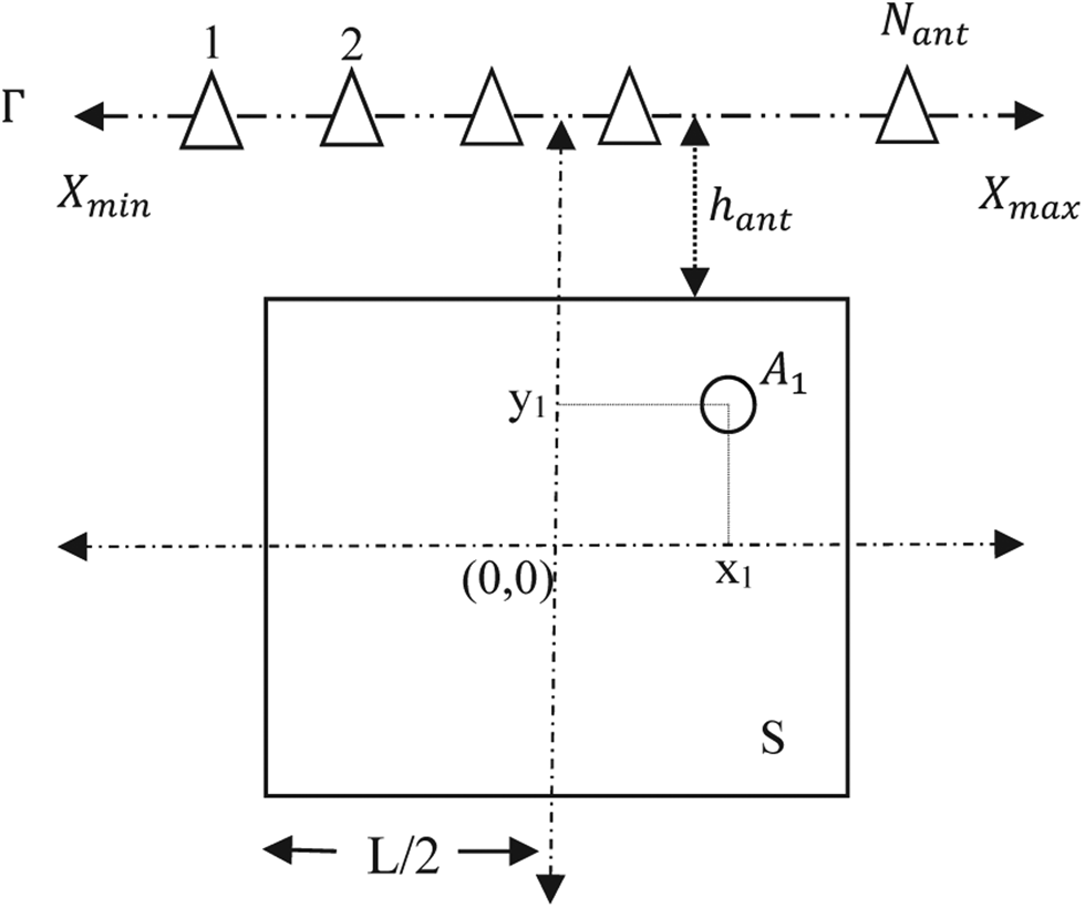
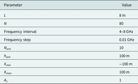
To illustrate the feasibility of the proposed algorithm, we consider a simulation scenario described in Fig. 1. For the sake of clarity, let us explain the source localization problem geometry shown in Fig. 1. The circular object is taken as the source and it is surrounded by another medium S. (x 1, y 1) are the coordinates of the point source having amplitude A 1. The remaining part of the problem geometry is modeled as a free space medium. N ant is the number of the receiving antennas which are on the line Γ and uniformly distributed with equal intervals. X min and X max are the minimum and maximum points of the line Γ. h ant is the distance between the line Γ and the medium S. Assume that the background medium is $S = [ -L/2 {\rm }\,m,\; L/2 {\rm }\,m] \times [ -L/2\, {\rm }m,\; L/2\, {\rm }m]$ . S domain is discretized into N × N points. The number and the position of the objects in the S domain can be changed for the purpose of the simulation. The simulation setup is generated and different scenarios of this setup are evaluated in the MATLAB environment. Operating frequency is linearly swept with 0.01 GHz steps and the scattered electrical field is registered at each position of the antenna. The simulation parameters given in Table I are used as default parameters for each scenario. If the effect of one of these parameters is desired to investigate on simulation, then the value of that parameter is varied while the values of the other simulation parameters are used as default. It is assumed that four point sources are considered in the measurements. The radiation amplitudes are selected as A 1 = A 2 = A 3 = A 4 = 1 from the aspect of simplicity of the scenarios. The coordinates of the sources were selected as [2 m, 2 m], [−3 m, −3 m], [2 m, −2 m], [−3 m, 3 m], respectively.
Configuration of the simulation (S: the background medium, A 1: amplitude of the circular source, Γ: measurement line, N ant: the number of the receiving antenna, h ant: the distance between the line Γ and the medium S, X min, and X max: the minimum and maximum point of the line Γ).

Default parameter values

Numerical results of the proposed method for multifrequency inverse source problem
In this section, several numerical results are proposed in order to demonstrate the capabilities and the limitations of the modified near-field FM for multifrequency inverse source problems. These simulation results include six different cases namely; central frequency, the length of receiving line, the number of receiving antennas, the distance between the line and the medium, relative amplitude effects, and comparison with a previous study.
Central frequency effect:
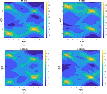
The purpose of this scenario is to show the accuracy of the proposed method in the simulation environment considering frequency intervals. The adopted frequency ranges in order to understand the central frequency effect are 2–6, 4–8, 6–10, and 8–12 GHz, respectively. As shown in Fig 2, it is observed that uncertainty behavior of the location of point sources decreases because of increasing the resolution as the central frequency increases in our simulations. Lastly, the proposed method can work with all microwave frequencies as long as the dimensions of the sources and their distances are accordingly chosen. In other words, for each problem, a suitable frequency band can be found according to the given dimensions.
Central frequency effect for (a) 2–6 GHz, (b) 4–8 GHz, (c) 6–10 GHz, (d) 8–12 GHz.

hant Effect:
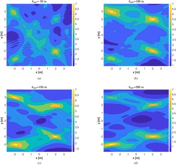
The effect of h ant to determine source localization is given in this scenario. It is shown that h ant directly affects the reconstruction of the objects from the results depicted in Fig. 3. When the value of h ant increases, a wider spread of the object image can be reconstructed in the bounded medium. We may also begin to lose the sensitive position of point sources. When the value of h ant parameter is increased, the resolution decreases as seen in Fig. 3.
h ant effect for (a) h ant = 50 m, (b) h ant = 100 m, (c) h ant = 150 m, (d) h ant = 200 m.

Nant Effect:
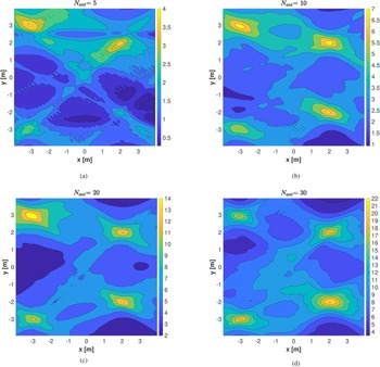
To further understand the effect of N ant on the simulation results, we choose the values of N ant from 5 to 30. When the number of receiving antennas increases, it is seen that the reconstruction of the objects can be better obtained as illustrated in Fig. 4.
N ant effect for (a) N ant = 5, (b) N ant = 10, (c) N ant = 20, (d) N ant = 30.

Xmin and Xmax Effect:
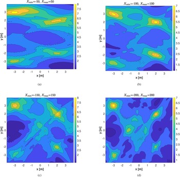
To better understand the capabilities of the presented method, the effect of X min and X max is investigated in Fig. 5. These parameters represent a length on which the antennas are equally spaced. It is concluded that the positions of reconstructed objects are acquired more precisely when X min and X max increase.
X min and X max effect for (a) X min = −50 m and X max = 50 m, (b) X min = −100 m and X max = 100 m, (c) X min = −150 m and X max = 150 m, (d) X min = −200 m and X max = 200 m.

Relative amplitude effect
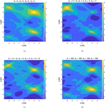
In order to illustrate the effect of different amplitudes of sources, we present four different cases as given in Fig. 6. Here, it is seen that the reconstructions of the targets are related with the data that can be taken from the target. Thus, as the amplitude increases and as the targets get closer to measurement antennas, they become well reconstructed and vice versa.
Effect of source amplitudes with (a) A 1 = 8, A 2 = 3, A 3 = 6, A 4 = 4; (b) A 1 = 0 + 2i, A 2 = 2, A 3 = 3, A 4 = 4; (c) A 1 = 0 + 4i, A 2 = 2, A 3 = 5, A 4 = 0 + 3i; (d) A 1 = 400, A 2 = 200, A 3 = 500, A 4 = 300.

Comparison results
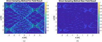
At last, the results of comparison of the presented method with a previous study that uses the DSM are reported [Reference Alzaalig, Hu, Liu and Sun38]. Firstly, we perform a reconstruction of the sources for multiple observation points with the method given in [Reference Alzaalig, Hu, Liu and Sun38]. We consider our scenario given in Fig. 2(b) and obtain both far and near-field imaging results of the DSM. When Fig. 7 is compared with Fig. 2(b), it is observed that the optimal result is Fig. 2(b), which is the introduced method, and then the second optimal is the far-field DSM in Fig. 7 and the worst one is the near-field DSM in Fig. 7.
(a) DSM [Reference Alzaalig, Hu, Liu and Sun38] far-field result for Fig 2(b) case. (b) DSM [Reference Alzaalig, Hu, Liu and Sun38] near-field result for Fig 2(b) scenario.

Conclusion
A modified near-field FM is presented for an electromagnetic source localization problem. An adapted factorization formulation is used for multifrequency inverse source problems with several and sparse near-field measurements. A different integral equation including incident angle and distance is obtained by employing an asymptotic approximation of Hankel's function. The abilities and restrictions of the modified formulations are tested in an electromagnetic source localization problem. To this aim, several different scenarios are used to explain the capabilities of the proposed method. Simulation results reveal that the presented method has an accurate and robust operation. This developed algorithm can be applied in 3D electromagnetic case, TE, and real near-field problems as further studies.
 N. Gökmen Karakiraz received his B.Sc. degree from Ankara University in 1997 and M.Sc. degree from Hacettepe University in 2010. He continues his Ph.D. studies at the National Defense University. His research interests include electromagnetic scattering, inverse source problem, and microwave imaging.
 A. Oktay Ertay received his B.Sc. degree in electronics and communication engineering from Yildiz Technical University, Istanbul, Turkey, in 2010 and M.Sc. and Ph.D. degree in telecommunication engineering from Istanbul Technical University (ITU), Istanbul, Turkey, in 2014 and 2019, respectively. He worked as a Research Assistant with Electronics and Communication Engineering Department, ITU, Istanbul, Turkey from 2011 to 2019. Now, he has been working as an Assistant Professor with Electrical Electronics Engineering Department, Erzincan Binali Yildirim University, Erzincan Turkey since 2019. He is co-recipient of 2016 IEEE Antennas and Propagation Ulrich L. Rohde Innovative Conference Paper Award of International Conference on Antenna Measurements & Applications Focus on Antenna Systems (CAMA) in Syracuse, USA. His current research interests include microwave imaging, electromagnetic bandgap structures, microwave circuits, slow wave structures, traveling wave tube amplifiers. He is a reviewer of several journals such as IEEE and IET.
 E. Göse received his B.Sc. degree from Turkish Air Force Academy (TurAFA) in 1992, M.Sc. degree from Bosphorus University of Istanbul in 2001, and Ph.D. degree from Yildiz Technical University of Istanbul, Turkey in 2005, all in Electrical Engineering. He is an Assistant Professor with the Department of Electronics Engineering, TurAFA. He was with Indiana Purdue Fort Wayne (IPFW) University, USA in 2010 for post doctoral study of one year. He became a professor in 2020. He performed research on wireless data acquisition and simulation of RF/microwave circuits. His research interests include wireless communication, channel coding, artificial neural network, genetics algorithm, RF, microwave and education.