
1. Introduction
Liquid metal batteries (LMBs) are high temperature electrochemical cells composed of three superposed layers of electrically conducting fluids of different densities (see sketch of figure 1a). The top layer is composed of a light metal (here Li), the middle layer is composed of a molten salt of higher density, and the bottom layer is composed of a heavy molten metal (here Pb). During discharge, the light metal ions from the top layer (here  $\textrm {Li}^+$) enter the molten salt. These ions then migrate towards the bottom of the salt layer and eventually enter the metal layer to form an alloy (here a Pb (Li) alloy). Contrary to what is assumed in most hydrodynamical studies on LMBs, the composition of the alloy layer is not constant in time. In particular, when the discharge is rapid, there is a local accumulation of light elements near the alloy–salt interface (see sketch of figure 1b) as diffusion of light elements into the alloy is slow: diffusivities of order
 $D \approx 10^{-8}\, \textrm {m}^2\ \textrm {s}^{-1}$ are considered to be realistic. The presence of an inhomogeneous alloy layer concentrated in light elements is detrimental to the operation of the battery: it lowers the delivered electrical potential and it may prematurely trigger the formation of solid intermetallics near the alloy–salt interface (Ning et al. Reference Ning, Phadke, Chung, Yin, Burke and Sadoway2015). In line with previous studies (Kelley & Sadoway Reference Kelley and Sadoway2014; Ashour & Kelley Reference Ashour and Kelley2018; Ashour et al. Reference Ashour, Kelley, Salas, Starace, Weber and Weier2018; Weber et al. Reference Weber, Nimtz, Personnettaz, Salas and Weier2018; Personnettaz et al. Reference Personnettaz, Landgraf, Nimtz, Weber and Weier2019; Herreman et al. Reference Herreman, Bénard, Nore, Personnettaz, Cappanera and Guermond2020; Weber et al. Reference Weber, Nimtz, Personnettaz, Weier and Sadoway2020), we investigate in this paper how swirling electrovortex flows occurring in the alloy can enhance the mixing therein and, hence, prevent the formation of the inhomogeneous alloy layer at the alloy–salt interface.
(a) We study the flow and composition of the bottom alloy layer of a discharging LMB. This layer is submitted to a uniform vertical magnetic field  $B_z$ and it is electrically connected from below to a thinner solid copper wire. The streamlines of the current density
 $\boldsymbol {j}$ show how the current is deviated towards the wire. (b) The Lorentz force is mainly azimuthal
 $- j_r B_z \boldsymbol {e}_\theta$ and always localized near the electrical contact. It generates a swirling electrovortex flow that pumps the material downwards in a spiral motion prior to ejecting it radially. The fluid motion is similar to that induced by a rotating impeller. We investigate how the swirling electrovortex flow enhances the mixing of the alloy that floats at the top of the cell and has a high lithium molar fraction.

As discussed in Weber et al. (Reference Weber, Nimtz, Personnettaz, Weier and Sadoway2020), the idea of using fluid motions to enhance mixing in the alloy layer of LMBs may be as old as LMBs themselves, but this idea has remained unexplored up until recently. This idea started to gain momentum in Kelley & Sadoway (Reference Kelley and Sadoway2014) where a fluid flow is generated in a liquid Pb(Bi) electrode by using the electrovortex mechanism and thermal convection. The magnitude of the velocity thus generated is measured in this reference by ultrasound techniques. The measured eddy turnover time then serves as a first-order estimate of the time needed to mix the alloy in the electrode. This experimental set-up has been studied numerically in various papers. In Ashour et al. (Reference Ashour, Kelley, Salas, Starace, Weber and Weier2018) the electrovortex flow and the thermal convection are investigated separately, and it is found therein that in some circumstances thermal convection can be slightly more intense than the electrovortex flow. Both types of forcing are considered simultaneously in Weber et al. (Reference Weber, Nimtz, Personnettaz, Salas and Weier2018). That paper also studies the effects of supplying the current with a wire that is perpendicular to the axis of the battery. The conclusion from these studies is that significant flows can be driven by thermal convection and by the electrovortex mechanism in liquid metal alloys. Moreover, in agreement with previous studies on the electrovortex mechanism (Millere, Sharamkin & Shcherbinin Reference Millere, Sharamkin and Shcherbinin1980; Bojarevičs & Shcherbinin Reference Bojarevičs and Shcherbinin1983; Bojarevics et al. Reference Bojarevics, Freibergs, Shilova and Shcherbinin1989; Davidson Reference Davidson1992; Ivochkin et al. Reference Ivochkin, Teplyakov, Guseva and Vinogradov2015; Kharicha et al. Reference Kharicha, Teplyakov, Ivochkin, Wu, Ludwig and Guseva2015; Vinogradov et al. Reference Vinogradov, Teplyakov, Ivochkin and Kharicha2018; Teplyakov et al. Reference Teplyakov, Vinogradov, Ivochkin and Klementyeva2018), these papers show that adding an external vertical magnetic field creates an electrovortex flow that rotates and is significantly more intense (this configuration is henceforth called a swirling electrovortex flow).
The first study that seeks to model mixing of the alloy layer in LMBs using the above mechanisms is due to Ashour & Kelley (Reference Ashour and Kelley2018). A prescribed stationary fluid flow, similar to a non-swirling electrovortex flow, and an advection–diffusion equation are used to model the alloy composition. A more precise model for the alloy motion and composition is introduced by Personnettaz et al. (Reference Personnettaz, Landgraf, Nimtz, Weber and Weier2019). This study is also the first to highlight the role of solutal buoyancy in the alloy motion. This effect was systematically neglected before. During the charging cycle, the alloy near the interface with the salt becomes locally heavier than its surroundings and rapidly plunges downwards giving rise to an intense solutal convection flow. This phenomenon is so strong that it is even active in very small LMBs. During a rapid discharge, solutal buoyancy has a strong stabilizing effect. The thin layer of light (here Li-enriched) alloy becomes lighter than the bulk and literally floats at the top of the alloy; see figure 1(b). The density difference can be as large as a few thousand  $\textrm {kg}\ \textrm {m}^{-3}$ (Herreman et al. Reference Herreman, Bénard, Nore, Personnettaz, Cappanera and Guermond2020). This is a very large number compared to what thermal buoyancy could create. In conclusion, solutal buoyancy radically changes the behaviour of the battery during charge and discharge. Solutal convection naturally mixes the alloy during charge. But during discharge, solutal buoyancy strongly opposes any vertical motion near the top of the alloy and thereby blocks dynamic mixing; hence, a sufficiently strong source of motion has to be found if one wants to enhance mixing.
Creating efficient motion in the alloy using thermal convection is not realistic. Previous studies on thermal convection in LMBs (Shen & Zikanov Reference Shen and Zikanov2016; Köllner, Boeck & Schumacher Reference Köllner, Boeck and Schumacher2017; Personnettaz et al. Reference Personnettaz, Beckstein, Landgraf, Köllner, Nimtz, Weber and Weier2018) suggest that the bottom alloy layer is in stable thermal stratification and that it is only weakly entrained by viscosity. Shen & Zikanov (Reference Shen and Zikanov2016) and Personnettaz et al. (Reference Personnettaz, Beckstein, Landgraf, Köllner, Nimtz, Weber and Weier2018) both report velocities in the alloy that are below  $1\, \textrm {mm}\ \textrm {s}^{-1}$ in a centimetre-scale device. This is likely not enough to both oppose solutal buoyancy and enhance mixing during discharge. On the other hand, the electrovortex mechanism is an interesting and fairly natural option to drive a fluid flow in the alloy.
In our first study (Herreman et al. Reference Herreman, Bénard, Nore, Personnettaz, Cappanera and Guermond2020) we have investigated the mixing capabilities of non-swirling electrovortex flows in LMBs. Referring to figure 1(b), the Lorentz force drives a predominantly poloidal electrovortex flow with  $u_\theta \approx 0$ when there is no external magnetic field (
 $B_z=0$). We have shown that this flow would be strong enough to influence the mixing of the alloy if solutal buoyancy were ignored. But the conclusion is entirely different when solutal buoyancy is accounted for. During charge, the electrovortex flow is overpowered by solutal convection. During discharge, the electrovortex flow is present in the bulk of the alloy, but it is unable to penetrate the layer of light alloy that forms at the alloy–salt interface and is therefore unable to enhance the mixing. Using basic physical arguments (energy balances), we have derived scaling laws for the intensity of the flow induced by solutal convection and for the mixing time during charge. For the more problematic case of discharge, we have estimated the magnitude of the velocity that is needed in a general bulk flow to overcome the solutal buoyancy effects. This model identifies two characteristic velocities
 $U_p$ and
 $U_m > U_p$ (see (1.1a,b)),
 \begin{equation} U_p= \left (\frac{2 {|J|} \mathcal{M}_{\textrm{Li}} \beta g H }{n_e F} \right )^{1/3} , \quad U_m = \left ( \frac{ 4 {|J|} \mathcal{M}_{\textrm{Li}} \beta g }{n_e F} \right)^{2/5} \frac{H^{3/5}}{ ({\rm \pi} D)^{1/5} }, \end{equation}
which only depend on the design parameters of the cell (height of the alloy layer  $H$, current density
 $J$), the properties of the charge carrier (for Li, the charge number
 $n_e=1$, the molar mass
 $\mathcal {M}_{\textrm {Li}}$), the alloy properties (solutal expansion coefficient
 $\beta$, binary diffusion coefficient
 $D$) and physical constants (
 $g$ gravity,
 $F$ Faraday constant). A bulk flow with a velocity magnitude
 $U$ such that
 $U \ll U_p$ is too weak to penetrate the stratified buoyant layer forming at the interface with the electrolyte. This type of flow cannot influence mixing. When
 $U \gg U_m$, the bulk flow is on the contrary intense enough to drag lightweight fluid parcels forming at the alloy–salt interface all around the cell and through the heavier bulk fluid, thereby making efficient mixing possible. In the intermediate range, i.e.
 $U \in [U_p, U_m]$, the flow can have a moderate effect on mixing, possibly only for a finite amount of time. The relevance of these velocity scales in the mixing problem has been supported by numerous numerical simulations in Herreman et al. (Reference Herreman, Bénard, Nore, Personnettaz, Cappanera and Guermond2020). Using this model together with a scaling law for the typical intensity
 $U$ of non-swirling electrovortex flows, we have verified that non-swirling electrovortex flows that are such that
 $U \ll U_p$ cannot enhance mixing during discharge.
In this paper we continue this investigation and focus our attention on swirling electrovortex flows. By allowing a background magnetic field  $B_z \boldsymbol {e}_z$ along the axis (green lines in figure 1a), the Lorentz force has an azimuthal component that is localized near the rim of the electrical contact between the alloy and the copper wire. This force distribution is reminiscent of that produced by a rotating impeller in a blender, as illustrated in figure 1(b). It has already been shown in Weber et al. (Reference Weber, Nimtz, Personnettaz, Weier and Sadoway2020) that swirling electrovortex flows can increase mixing in the alloy layer during discharge, despite the stabilizing effects of solutal buoyancy. We confirm this here and also offer some physical arguments identifying what is actually needed to enhance mixing with swirling electrovortex flows. The paper is structured as follows. We introduce the problem and the model investigated in the paper in § 2. We also briefly describe in this section the numerical technique that we use. Then we numerically demonstrate in § 3 that enhanced mixing can be achieved by using the swirling electrovortex mechanism. Some of the three-dimensional simulations are extremely challenging as the Reynolds (and Péclet number) can reach very high values and transition to turbulence occurs. In § 4 we use numerical simulations and theoretical arguments to derive a novel scaling law for the intensity of the electrovortex. Using this scaling law, we then derive a theoretical estimate for the minimal external magnetic field
 $B_z$ that is needed to enhance mixing in LMB alloys using swirling electrovortex flows. We finally combine this scaling law with the criterion for efficient mixing,
 $U\gg U_m$, derived in Herreman et al. (Reference Herreman, Bénard, Nore, Personnettaz, Cappanera and Guermond2020) to find the minimal external magnetic field strength that yields enhanced mixing. Our numerical simulations show that this criterion is accurate.
2. Model
We consider a Li $||$Pb LMB in discharge mode. We use the same model as in Herreman et al. (Reference Herreman, Bénard, Nore, Personnettaz, Cappanera and Guermond2020) to describe the flow and the composition of the Pb(Li) alloy in the positive electrode of the battery. We denote
 $R$ the radius of the cylindrical cell and
 $H$ the height of the alloy layer. We neglect the slow time variation of
 $H$ during discharge. In the fluid domain we solve the Boussinesq model
 \begin{gather} \rho_* ( \partial_t \boldsymbol{u} + (\boldsymbol{u} \boldsymbol{\cdot} \boldsymbol{\nabla}) \boldsymbol{u} ) ={-} \boldsymbol{\nabla} p - ( \rho_* - \chi (\rho_\textrm{Li} - \rho_{\textrm{Li},*})) g \boldsymbol{e}_z \nonumber\\ \hspace{11pc} + \boldsymbol{\nabla} \boldsymbol{\cdot} \left ( \rho_* \nu \left ( \boldsymbol{\nabla} \boldsymbol{u} + (\boldsymbol{\nabla} \boldsymbol{u})^{\textsf{T}} \right ) \right ) + \boldsymbol{j} \times \boldsymbol{b}, \end{gather}
 \begin{gather} \partial_t \boldsymbol{b} = \boldsymbol{\nabla} \times (\boldsymbol{u} \times \boldsymbol{b}) +(\mu_0 \sigma)^{{-}1} \Delta \boldsymbol{b} , \end{gather}
 \begin{gather}\boldsymbol{\nabla} \boldsymbol{\cdot} \boldsymbol{u} = 0 , \quad \boldsymbol{\nabla} \boldsymbol{\cdot} \boldsymbol{b} = 0, \end{gather}
 \begin{gather}\partial_t \rho_\textrm{Li} + \boldsymbol{u} \boldsymbol{\cdot} \boldsymbol{\nabla} \rho_\textrm{Li} = D \, \boldsymbol{\nabla}^2 \rho_\textrm{Li}. \end{gather}
Here  $\boldsymbol {u}$ is the velocity,
 $p$ is the pressure,
 $\boldsymbol {b}$ is the magnetic induction,
 $\boldsymbol {j} = \mu _0^{-1} \boldsymbol {\nabla } \times \boldsymbol {b}$ is the current density and
 $\rho _\textrm {Li}$ is the mass concentration of Li in the alloy. We denote
 $g$ gravity and
 $\mu _0$ the vacuum magnetic permeability. The reference densities
 $(\rho _*,\rho _{\textrm {Li},*})$ correspond to the eutectic alloy with the molar fraction
 $x_\textrm {Li} = 17\,\%$. The linear variation of the density with respect to
 $\rho _\textrm {Li}$ is obtained from an experimental result (Khairulin et al. Reference Khairulin, Abdullaev, Stankus, Agazhanov and Savchenko2016),
 \begin{align} \rho \approx \rho_* - \chi (\rho_\textrm{Li} - \rho_{\textrm{Li},*}) \quad \mbox{with}\ \begin{cases} \rho_* = 9543\ \textrm{kg} \ \textrm{m}^{{-}3},\\ \rho_{\textrm{Li},*} = 65\ \textrm{kg} \ \textrm{m}^{{-}3}, \end{cases} \quad \chi ={-} \textrm{d} \rho / \textrm{d} \rho_\textrm{Li} =15.1. \end{align}
As an alternative to  $\chi$, one can use the solutal expansion coefficient
 $\beta = \chi / \rho _* =1.58\times 10^{-3} \, \textrm {m}^3 \ \textrm {kg}^{-1}$. The kinematic viscosity,
 $\nu$, electrical conductivity,
 $\sigma$, and diffusion coefficient,
 $D$, are held fixed at their eutectic alloy values, i.e.
 \begin{equation} \nu \approx 1.44 \times 10^{{-}7} \ \textrm{m}^2 \ \textrm{s}^{{-}1} , \quad \sigma \approx 7.39 \times 10^{5} \ \textrm{S}\ \textrm{m}^{{-}1} , \quad D = 8 \times 10^{{-}9}\ \textrm{m}^2\ \textrm{s}^{{-}1}. \end{equation}
The fluid domain is connected from below to a solid copper wire of radius  $R_w$ and height
 $H_w$. In this wire, we solve the magnetic induction equation
 \begin{equation} \partial_t \boldsymbol{b}_w = (\mu_0 \sigma_w)^{{-}1} \Delta \boldsymbol{b}_w, \quad \boldsymbol{\nabla} \boldsymbol{\cdot} \boldsymbol{b}_w = 0. \end{equation}
We use the conductivity of copper,  $\sigma _w = 5.96 \times 10^{7} \, \textrm {S}\ \textrm {m}^{-1}$.
The no-slip boundary condition is enforced everywhere on the velocity. This condition is actually an approximation at the interface between the molten salt layer and the alloy layer,  $\{z=H\}$. This boundary condition has been shown in Herreman et al. (Reference Herreman, Bénard, Nore, Personnettaz, Cappanera and Guermond2020) to be a good approximation for non-swirling electrovortex flows. In the case under consideration here where the flow undergoes a swirling motion about the vertical axis, the salt layer should be entrained in a very slow rotation, but we do not expect that neglecting this effect significantly alters the flow or the alloy composition. The electrical boundary conditions are
 \begin{gather} (b_r, b_\theta ) |_{z=H} = (0, \mu_0 J r / 2) , \quad (b_\theta,b_z ) |_{r=R} = (\mu_0 J R / 2,B_z), \end{gather}
 \begin{gather}(b_r, b_\theta ) |_{z=0} = (0, \mu_0 J R^2 / 2 r) \ \forall r \in [R_w,R], \end{gather}
 \begin{gather}\boldsymbol{e}_z \times ( \boldsymbol{b} - \boldsymbol{b}_w ) |_{z=0} = 0 , \quad \boldsymbol{e}_z \times ((\kern1.5pt \boldsymbol{j}/ \sigma) - (\kern1.5pt \boldsymbol{j}_w / \sigma_w) ) |_{z=0} = 0 , \quad \forall r \in [0, R_w], \end{gather}
 \begin{gather}(b_{w,\theta},b_{w,z} ) |_{r=R_w} = ( \mu_0 J R^2 / 2 R_w, B_z), \end{gather}
 \begin{gather}(b_{w,r},b_{w,\theta} ) |_{z={-}H_w} = (0, \mu_0 J R^2 r / 2 R_w^2 ). \end{gather}
These boundary conditions are suitable in the low magnetic Reynolds number regime (see discussion in last paragraph of § III.A of Herreman et al. Reference Herreman, Nore, Ziebell Ramos, Cappanera, Guermond and Weber2019b). Note that it is through these boundary conditions that we impose the external  $B_z$, see (2.2a) and (2.2d). There is no external magnetic field in Herreman et al. (Reference Herreman, Bénard, Nore, Personnettaz, Cappanera and Guermond2020). Concerning the boundary conditions for
 $\rho _\textrm {Li}$, we consider that the side and the bottom boundaries are impermeable to Li (i.e. the mass flux is zero there). The mass flux of Li is imposed at the top surface (i.e. the interface with the electrolyte),
 \begin{equation} D\partial_r \rho_\textrm{Li} |_{r=R} = 0 , \quad D\partial_z \rho_\textrm{Li} |_{z=0} = 0 , \quad D\partial_z \rho_\textrm{Li} |_{z=H} ={-} \frac{J \mathcal{M}_\textrm{Li} }{n_e F }. \end{equation}
In this formula  $\mathcal {M}_{\textrm {Li}} = 6.941 \times 10^{-3} \, \textrm {kg}\ \textrm {mol}^{-1}$ is the molar mass of lithium,
 $n_e =1$ is the number of charges carried by the lithium ions, and
 $F=96485 \, \textrm {s} \ \textrm {A} \ \textrm {mol}^{-1}$ is the Faraday constant. The mass flux of
 $\textrm {Li}$ at the electrolyte interface is positive during discharge
 $(J<0)$.
As an initial condition, the fluid is at rest, i.e.  $\boldsymbol {u}=0$, and
 $\rho _\textrm {Li}=\rho _{\textrm {Li},*}$. The initial condition for the magnetic field is less important than the initial conditions on the velocity and the molar fraction as the magnetic field almost immediately adjusts due to the high magnetic diffusion.
We solve this problem using the massively parallel numerical code SFEMaNS, previously described in Guermond et al. (Reference Guermond, Laguerre, Léorat and Nore2007, Reference Guermond, Laguerre, Léorat and Nore2009), Cappanera et al. (Reference Cappanera, Guermond, Herreman and Nore2018) and used in the LMB context in Herreman et al. (Reference Herreman, Nore, Cappanera and Guermond2015, Reference Herreman, Nore, Guermond, Cappanera, Weber and Horstmann2019a,Reference Herreman, Nore, Ziebell Ramos, Cappanera, Guermond and Weberb, Reference Herreman, Bénard, Nore, Personnettaz, Cappanera and Guermond2020). All the fields are decomposed on a Fourier basis in the azimuthal direction and finite element bases in the meridian plane. As an example, we expand the velocity field as
 \begin{equation} \boldsymbol{u} = \sum_{m=0}^{M-1}\boldsymbol{u}_m^c (r,z,t) \cos (m \theta) + \sum_{m=1}^{M-1}\boldsymbol{u}_m^s (r,z,t) \sin (m \theta). \end{equation}
Here  $\boldsymbol {u}_m^c (r,z,t)$ and
 $\boldsymbol {u}_m^s (r,z,t)$ are time-dependent quadratic finite element functions and
 $m$ is the azimuthal wavenumber. The code is parallelized using domain decomposition in the meridian plane and along the different Fourier modes. A noticeable advantage of SFEMaNS is that axisymmetric simulations and three-dimensional (3-D) simulations can be performed on the same configuration. Throughout the paper, we use several global diagnostics. For the molar fraction, we use
 \begin{equation} \langle x_{\textrm{Li}} \rangle_S = \frac{1}{{\rm \pi} R^2} {\int_S} x_{\textrm{Li}} |_{z=H} \, \mathrm{d} S , \quad \langle x_{\textrm{Li}} \rangle_V = \frac{1}{{\rm \pi} R^2 H} {\int_V} x_\textrm{Li} \, \mathrm{d}V. \end{equation}
The notation  $\langle \ldots \rangle _V$ indicates a volume average. For the flow, we use the root mean square (r.m.s.) velocity and the maximal velocity in the volume
 \begin{equation} u_{{rms}} = \sqrt{\langle \| \boldsymbol{u}^2\| \rangle_V}, \quad u_{max} = \max_{\boldsymbol{x} \in V} \| \boldsymbol{u}\|. \end{equation}
To isolate the axisymmetric part of the r.m.s. velocity, we introduce
 \begin{equation} u_{{axi}} = \sqrt{u_{{tor}}^2 + u_{{pol}}^2 }, \quad u_{{{tor}}} = \sqrt{\langle (u_{0,\theta}^c)^2 \rangle_V }, \quad u_{{pol}} = \sqrt{\langle (u_{0,r}^c)^2 + (u_{0,z}^c)^2\rangle_V}. \end{equation}
Here the indices  $_{tor}$ and
 $_{pol}$ refer to the toroidal (along
 $\theta$) and the poloidal (along
 $r,z$) parts of the velocity. Note that in axisymmetric simulations
 $u_{{rms}} = u_{{axi}}$. To keep track of the non-axisymmetric part of the flow in the 3-D simulations, we also compute
 \begin{equation} u_{\text{3D}} = \sqrt{u_{{rms}}^2- u_{{axi}}^2}. \end{equation}
We report in table 1 important parameters that have been used in the numerical simulations done for this paper. More precisely, we give in this table the maximal number of Fourier modes,  $M$, the typical meridian mesh size and the time step,
 $\Delta t$, for every figure shown in the paper.
Details on the numerical simulations discussed in this article. Referring to each figure, we provide the number of Fourier modes,  $M$, the interval of (non-uniform) mesh sizes of the finite element grid in the meridian plane. The time step
 $\Delta t$ is fixed but sometimes needs to be lowered after checkpoints/restarts to maintain stability. Intervals
 $\Delta t_1 \rightarrow \Delta t_2$ indicate that
 $\Delta t$ was progressively decreased at various checkpoints.

3. Demonstrating the possibility of enhanced mixing in a small cell
In a first series of simulations we demonstrate the feasibility of enhanced mixing by means of the swirling electrovortex mechanism. This has already been done in Weber et al. (Reference Weber, Nimtz, Personnettaz, Weier and Sadoway2020) in a small realistic LMB set-up with a very thin alloy layer ( $R=4.45 \, \textrm {cm}, H=0.28 \, {\textrm {cm}}$). Here we investigate the idealized cell considered in our previous study (Herreman et al. Reference Herreman, Bénard, Nore, Personnettaz, Cappanera and Guermond2020). The geometry is
 $(H,R,H_w,R_w)=(2,4,4,0.8)\, {\textrm {cm}}$. All the simulations are done in the discharge scenario, i.e.
 $J< 0$. Somewhat arbitrarily we also use
 $B_z<0$ which creates a negative swirl (predominantly
 $u_\theta < 0$). Simulations with
 $B_z > 0$ would give a velocity field that swirls in the opposite direction (predominantly
 $u_\theta > 0$) but with the same radial and vertical components
 $u_r$,
 $u_z$.
3.1. Axisymmetric simulations
We first present axisymmetric simulations. Three-dimensional computations are discussed later. We impose the density current  $J=-5\, \textrm {kA} \ \textrm {m}^{-2}$ and vary
 $B_z$ in the range
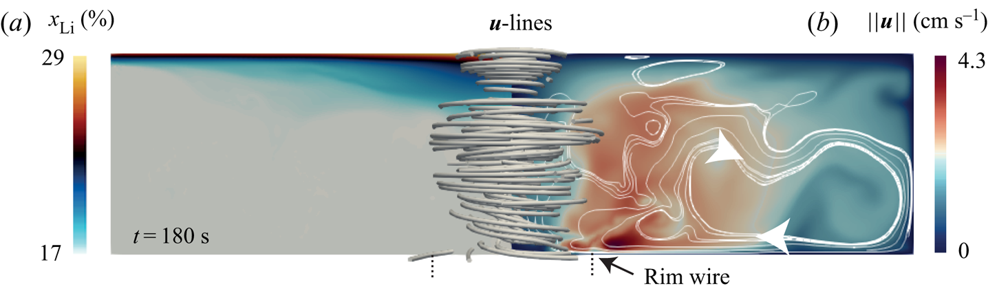
 $-[1,10] \, {\textrm {mT}}$. We show in figure 2 the molar fraction distribution and the velocity field obtained at
 $t= 20\, {\textrm {s}}$ with the lowest magnetic field
 $B_z = -1 \, {\textrm {mT}}$. The molar fraction is shown in the left panel. The magnitude of the velocity field and some streamlines are shown in the right panel of the figure. We observe in the left panel that the fluid flow generated by the swirling electrovortex is not strong enough to prevent the formation of a buoyant layer at the top of the electrode. In this layer the molar fraction
 $x_{\textrm {Li}}$ is stratified and reaches high values at the interface with the electrolyte. The fluid flow is time dependent and has a strong azimuthal component as suggested by the 3-D streamlines. The magnitude of the velocity is close to
 $4.3 \, \textrm {cm}\ \textrm {s}^{-1}$ and, as discussed in the introduction, it is maximal at the rim of the electrical contact with the wire.
Molar fraction  $x_\textrm {Li}$ (a) and velocity magnitude
 $\| \boldsymbol {u} \|$ (b) in the meridian section at
 $t= 100 \ {\textrm {s}}$ with
 $J = - 5\ \textrm {kA} \ \textrm {m}^{-2}$ and
 $B_z = - 1\ {\textrm {mT}}$. Streamlines of the velocity field near the
 $z$-axis are also shown.

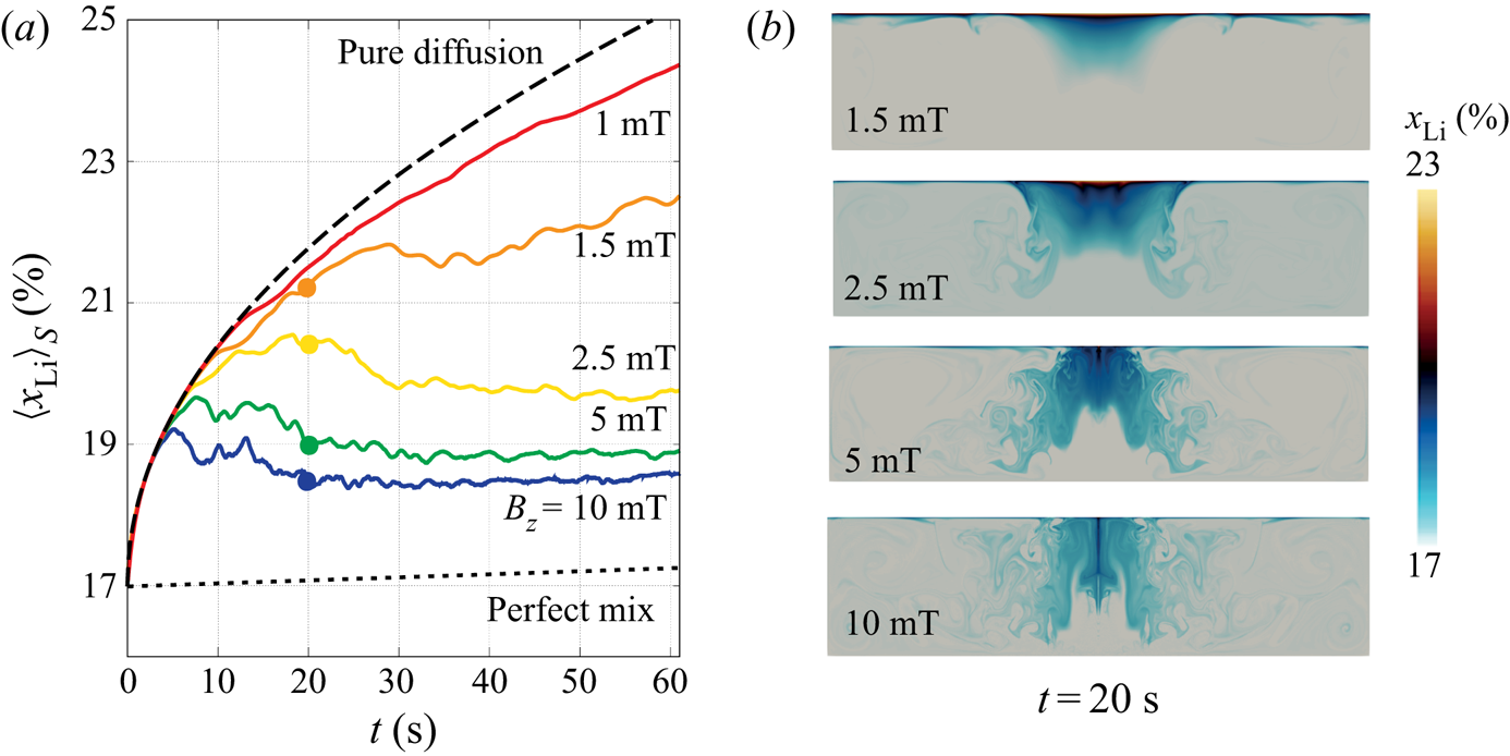
A small increase in the value of the magnetic field strength  $B_z$ significantly changes the blending capabilities of the flow. This is demonstrated in the left panel of figure 3, where we display the surface averaged molar fraction
 $\langle x_{\textrm {Li}} \rangle _S$ at the top interface as a function of time (see (2.5a,b)). For comparison, we have added in the figure two theoretical limit behaviours discussed in Herreman et al. (Reference Herreman, Bénard, Nore, Personnettaz, Cappanera and Guermond2020). The dotted line shows the time evolution of the molar fraction that would be observed if the alloy were mixed instantaneously throughout the bulk. The dashed line shows the time evolution of the molar fraction that would be observed if only diffusion were acting. With the magnetic field
 $|B_z| = 1 \, {\textrm {mT}}$, the time evolution of
 $\langle x_{\textrm {Li}}\rangle _S$ remains close to the diffusive line, indicating poor mixing. When the magnetic field intensity is large enough, say
 $|B_z| \geqslant 2.5 \, {\textrm {mT}}$, the surface averaged molar fraction
 $\langle x_{\textrm {Li}} \rangle _S$ initially follows the diffusive line, but after a short transient, it significantly drops down and eventually follows a path parallel to the ideal scenario where the alloy is perfectly mixed. This is a sign that mixing in the alloy has been greatly enhanced. We show in the right panel of the figure the distribution in the meridian section of the molar fraction
 $x_\textrm {Li}$ at
 $t=20\, {\textrm {s}}$ for different values of
 $B_z$. These snapshots clearly show that the homogeneity of the alloy improves as
 $|B_z|$ increases.
Influence of the swirling electrovortex flow on the molar fraction of  $\textrm {Li}$ with
 $J = -5 \, \textrm {kA}\ \textrm {m}^{-2}$ and
 $B_z\in \{-1,-1.5,-2.5,-5,-10\}\, {\textrm {mT}}$. (a) Time evolution of
 $\langle x_{\textrm {Li}} \rangle _S$. The influence of the electrovortex flow is clear for magnetic field intensities greater than
 $|B_z| = 1 \, {\textrm {mT}}$. (b) Snapshots of the molar fraction
 $x_\textrm {Li}$ distribution in the meridian section at
 $t= 20\, {\textrm {s}}$.

We show in figure 4 three snapshots of the molar fraction and the magnitude of the velocity field at  $t=4$,
 $t=8$ and
 $t=12\, \textrm {s}$ with
 $B_z = -5 \, {\textrm {mT}}$. A movie of this sequence for
 $t\in [0,12 ]\, {\textrm {s}}$ with intervals of
 $0.1\, {\textrm {s}}$ is provided in the supplementary material (movie 1 (velocity
 $||\boldsymbol {u}||$) and movie 2 (molar fraction
 $x_\textrm {Li}$)). At
 $t=4 \, {\textrm {s}}$ the velocity field rotates rapidly in the region close to the junction with the copper wire. This rotation creates a centrifugal pressure drop near the vertical axis of the cell, which in turn pumps the fluid downwards along a conical path (white arrows) prior to expelling it radially. This motion is also visible on the
 $x_\textrm {Li}$ distribution on the left panels of the figure, where the light alloy is clearly being dragged downwards from the top of the electrode into the bulk. The sharp change of the magnitude of the velocity
 $\|\boldsymbol {u}\|$ near the axis is indicative of a shear layer (with conical shape). This layer is unstable and a Kelvin–Helmholtz instability develops over time. Vortex rings are clearly visible at
 $t=8 \, {\textrm {s}}$ on both the molar fraction distribution
 $x_\textrm {Li}$ and the velocity magnitude
 $\|\boldsymbol {u}\|$ distribution. These vortex rings strongly interact and cause large fluctuations in the velocity field which greatly help the mixing. In the snapshot at
 $t=12 \, {\textrm {s}}$, we observe structures reminiscent of Taylor–Proudman columns in the bulk.
Snapshots at  $t=4\, {\textrm {s}}$,
 $t=8\ {\textrm {s}}$ and
 $t=12\, {\textrm {s}}$ of the molar fraction
 $x_{\textrm {Li}}$ (a) and velocity magnitude
 $\| \boldsymbol {u}\|$ (b) with
 $J= - 5 \, \textrm {kA}\ \textrm {m}^{-2}$ and
 $B_z = -5 \, {\textrm {mT}}$. The fluid is pumped downwards prior to being radially expelled as an impeller would do. This flow is very efficient at blending the alloy and prevents large inhomogeneities to build up near the interface with the electrolyte. See also movies 1 and 2 in the supplementary material available at https://doi.org/10.1017/jfm.2021.79.

3.2. Three-dimensional simulations
We now numerically investigate how three dimensionality affects the swirling electrovortex flow and its mixing properties. We focus on the parameters  $J=-5 \, \textrm {kA}\ \textrm {m}^{-2}$ and
 $B_z = - 5 \, {\textrm {mT}}$ which the axisymmetric simulations show mix well the alloy. With velocities of order
 $U \approx 5\, \textrm {cm}\ \textrm {s}^{-1}$, the Reynolds number
 $Re = U R / \nu$ is approximately
 $Re \approx 14\,000$; as a result, transition to turbulence must occur after some transient. The low value of the diffusivity
 $D = 8 \times 10^{-9} \, \textrm {m}^2\ \textrm {s}^{-1}$ is more problematic for the Péclet number
 $Pe = U R / D$ when it reaches values as high as
 $Pe\approx 2.5 \times 10^{5}$. This means that one must expect to see scales as small as
 $\sqrt {DR/U} \approx 0.08 \, {\textrm {mm}}$ in the
 $\rho _{\textrm {Li}}$-distribution (scale at which diffusion balances fluid parcel stretching). Axisymmetric simulations can resolve this scale, but 3-D simulations that are fully resolved down to this scale are not possible with the resource available to us. Hence, starting from an axisymmetric state, we only simulate the initial transient phase of the three dimensionalization before turbulence fully develops. We use a fine meridian mesh that contains
 $86\times 10^3$ points and
 $M=128$ complex Fourier modes (i.e. 256 real Fourier modes). At the end of the simulation the time step is
 $\Delta t= 2.5 \times 10^{-5}\, \textrm {s}$. The maximal time reached in the 3-D simulations is
 $t= 18.375\, \textrm {s}$. After this time, the filaments in the molar fraction
 $x_{\textrm {Li}}$ become so thin that they can no longer be correctly resolved and numerical instabilities occur.
In figure 5 we compare the axisymmetric and 3-D simulations. We show in figure 5(a) the time evolution of the surface averaged molar fraction  $\langle x_{\textrm {Li}} \rangle _S$. We observe that the mixing properties of the 3-D flow are slightly affected by three dimensionality. The mixing seems to be slightly less efficient in three dimensions, but the 3-D simulation is probably too short to draw a definitive conclusion in this respect. The snapshots of the molar fraction distribution in figure 5(b) show that the mixing is intense both in the axisymmetric and in the 3-D simulations. In movie 3 of the supplementary material one can see the evolution of the molar fraction
 $x_\textrm {Li}$ in the 3-D simulation through time. We show in figure 5(c) the time evolution of the r.m.s. velocities
 $u_{{axi}}$ and
 $u_{\text {3D}}$ (defined in (2.7a–c) and (2.8)). The non-axisymmetric part of the flow,
 $u_{\text {3D}}$, rapidly grows at about
 $t= 12 \, {\textrm {s}}$ and in about just
 $6\, {\textrm {s}}$ reaches a significant level
 $u_{\text {3D}} = 0.12 u_{{axi}}$. Notice though that the axisymmetric part of the r.m.s. velocity in the 3-D simulation,
 $u_{{axi}}$, is almost identical to that from the axisymmetric simulation. We show snapshots of
 $\|\boldsymbol {u}\|$ in figure 5(d). The 3-D flow is turbulent but remains comparable to the axisymmetric flow.
Comparison of 3-D and axisymmetric simulations for  $J=-5\, \textrm {kA}\ \textrm {m}^{-2}$ and
 $B_z=-5\, {\textrm {mT}}$. (a) Surface averaged molar fraction as a function of time. (b) Snapshots of the molar fraction at similar times in
 $x=0$ plane and
 $z=2 \, {\textrm {cm}}$ plane. (c) Root mean square velocities as a function of time. (d) Snapshots of the flow speed at similar times in
 $x=0$ plane and
 $z=1.98 \, {\textrm {cm}}$ plane. In movie 3 of the supplementary material, one can observe a sequence of
 $x_{\textrm {Li}}$ in the 3-D simulation at different times.

In figure 6 we show horizontal slices of the 3-D molar fraction distribution at the heights  $z\in \{1.98, 1.5, 1,0.5\} \, {\textrm {cm}}$ at the final time
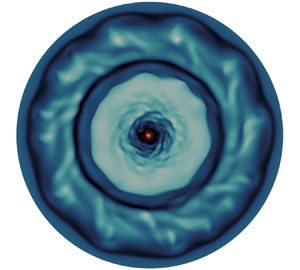
 $t=18.375 \, {\textrm {s}}$. The graphical abstract shows the
 $x_\textrm {Li}$ distribution at time
 $t=16\, {\textrm {s}}$ at the same height. Recalling that
 $H=2\, {\textrm {cm}}$, and since the diffusive length scale is about
 $\sqrt {D t} = 0.04 \, {\textrm {cm}}$, the slice at
 $z=1.98\, {\textrm {cm}}$ in figure 6(a) is within the thin stratified boundary layer that forms by diffusion at the top of the alloy. In movie 4 of the supplementary material we can clearly observe how spiraling waves appear after some
 $15\, {\textrm {s}}$; we conjecture that they are the consequence of shear-type instabilities that are also observed in rotor-stator experiments (Gauthier et al. Reference Gauthier, Gondret, Moisy and Rabaud2002). The three slices at
 $z\in \{1.5, 1,0.5\} \, {\textrm {cm}}$ in figure 6(b) clearly demonstrates that the molar fraction distribution is three dimensional. The size of the finest filaments in these figures is close to the mesh size. Long time 3-D simulations with
 $Pe> 10^5$ when turbulence is fully developed would require either finer grids (too expensive at the moment) or some kind of turbulence modelling or stabilization.
Horizontal slices of molar fraction  $x_\textrm {Li}$ in 3-D simulation with
 $J=-5\, \textrm {kA}\ \textrm {m}^{-2}$,
 $B_z=-5\, {\textrm {mT}}$ at
 $t=18.375 \, {\textrm {s}}$ and at different heights. (a) Just below the top surface at
 $z=1.98\, {\textrm {cm}}$ we are in the stratified boundary and we observe spiraling structures. The notation
 ${>}$19 means that the colour scale is slightly saturated for a better contrast,
 $x_{\textrm {Li}}$ can locally exceed
 $19\,\%$ (b) at heights
 $z=1.5, 1, 0.5\, {\textrm {cm}}$. In the supplementary material we provide a movie for
 $x_{\textrm {Li}}$ at height
 $z=1.98 \, {\textrm {cm}}$ in the 3-D simulation (movie 4).

The 3-D simulation is too short to conclude unequivocally on the mixing properties of the 3-D flow at late times, but it nevertheless shows that mixing is very intense. Whether mixing is as efficient in three dimensions as in axisymmetric simulations is not clear. Another important point here is that this 3-D simulation demonstrates that the axisymmetric simulations provide good estimates of the mixing capabilities of the swirling electrovortex flow.
In appendix B we further compare the axisymmetric and the 3-D simulations with a diffusivity that is ten times higher  $D_{relax} = 10 D = 8 \times 10^{-8} \, \textrm {m}^2\ \textrm {s}^{-1}$ (
 $J$ and
 $B_z$ being unchanged). The actual value of the diffusion coefficient is anyway somewhat uncertain as it depends on the temperature and the alloy composition (Khairulin, Stankus & Abdullaev Reference Khairulin, Stankus and Abdullaev2017), and it might indeed be higher than the very small value
 $D = 8 \times 10^{-9} \, \textrm {m}^2\ \textrm {s}^{-1}$ that we have used here. With this value of the diffusivity the overall structure of the fluid flow is fairly similar, but the spiraling wave-like structures are more clearly visible near the top of the alloy. Interestingly, we also observe that the time evolution of the surface averaged molar fraction
 $\langle x_{\textrm {Li}} \rangle _S$ for the 3-D and axisymmetric flows are very close; see figure 13(a). With increased diffusion, mixing is made easier and the density variations in the stratified layer at the top of the alloy are smaller. It is then easier for the bulk flow to reach through the stratified layer and enhance mixing therein.
4. Minimal magnetic field strength to enhance mixing
Having demonstrated that mixing of the alloy in the bottom electrode can be greatly improved during discharge, we now want to identify the physical conditions that are really required in order to enhance the mixing. We answer this question in two steps. First we look for a scaling law for the magnitude of the velocity in the swirling electrovortex flow. Then, we estimate the minimal magnetic field intensity that is needed to enhance the mixing during discharge by combining the velocity scaling law with the characteristic velocities  $U_p$ and
 $U_m$ introduced by Herreman et al. (Reference Herreman, Bénard, Nore, Personnettaz, Cappanera and Guermond2020).
4.1. Scaling law for the intensity of swirling electrovortex flows
In this section we estimate the intensity  $U$ of the electrovortex flow in terms of the input parameters
 $J$ and
 $B_z$. We first identify a scaling law using numerical simulations, then we propose theoretical arguments to explain the origin of this behaviour.
4.1.1. Numerical evidence
The flow is steady and axisymmetric for small values of  $JB_z$ (Millere et al. Reference Millere, Sharamkin and Shcherbinin1980). But, as explained in appendix A, as
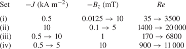
 $JB_z$ increases the flow first bifurcates to an unsteady regime, and eventually bifurcates to a time-dependent 3-D regime. Although axisymmetric solutions are not realistic at large Reynolds numbers, we have seen in the previous section that on average the velocity field is very similar to that observed in 3-D simulations. We then posit that axisymmetric simulations provide accurate estimates of the mean magnitude of the actual 3-D flow. We have done four sets of axisymmetric simulations to explore the parameter domain covered by the pair
 $(J,B_z)$. These four sets are described in table 2. In the set labelled (i) we set the current to the low value
 $J=-0.5\, \textrm {kA}\ \textrm {m}^{-2}$ and let
 $B_z$ vary in the interval
 $[0.125,10]\, {\textrm {mT}}$. In set (ii) we set the current to the large value
 $J=-10\, \textrm {kA}\ \textrm {m}^{-2}$ and let
 $B_z$ vary in the interval
 $[0.1,5]\, {\textrm {mT}}$. In set (iii) we set the magnetic field to the low value
 $B_z=1\, {\textrm {mT}}$ and let
 $J$ vary in the interval
 $[0.5,10]\, \textrm {kA}\ \textrm {m}^{-2}$. In set (iv) we set the magnetic field to the large value
 $B_z=10\, {\textrm {mT}}$ and let
 $J$ vary in the interval
 $[0.5,5]\, \textrm {kA}\ \textrm {m}^{-2}$. We ignore the buoyancy effects in all these simulations, i.e. we set
 $g=0$ in (2.1a). For each simulation, we denote by
 $\bar {u}_{{rms}}$ the time-averaged r.m.s. of the magnitude of the computed velocity (see (2.6a,b)). This quantity allows us to define the Reynolds number
 \begin{equation} Re = \frac{\bar{u}_{{rms}} R}{\nu}. \end{equation}
The range covered by the Reynolds number for each data set is shown in table 2.
Ranges for  $J$ and
 $B_z$ in the axisymmetric simulations. The Reynolds number
 $Re = \bar {u}_{{rms}} R / \nu$ is based on the time-averaged r.m.s. speed obtained from the simulations.

We show in figure 7(a) the time-averaged r.m.s. speeds  $\bar {u}_{{tor}}$ and
 $\bar {u}_{{pol}}$ as functions of the parameters
 $B_z$ and
 $J$ for the four data sets (i), (ii), (iii), (iv). In most cases, we observe a power-law behaviour in which
 $\bar {u}_{{tor}} \sim \bar {u}_{{pol}} \sim (J B_z)^{2/3}$. We also notice that the toroidal (azimuthal) component of the velocity is typically five times more intense than the poloidal component, which also implies that
 $\bar {u}_{{rms}} \approx \bar {u}_{{tor}}$. In figure 7(b) we replot
 $\bar {u}_{{tor}}$ as a function of
 $({JB_z}/{\rho _*})^{2/3}\nu ^{-1/3} R$ for all the data points. Setting
 $U = \bar {u}_{{tor}} \approx \bar {u}_{{rms}}$, we observe that the scaling law
 \begin{equation} U \sim \left ( \frac{J B_z}{\rho_*} \right )^{2/3} \frac{R}{\nu^{1/3}} \end{equation}
is valid over almost three decades. Several points are marked with a star because they deviate from this scaling law. An explanation for these discrepancies is proposed below in § 4.1.3.
Scaling laws for the quantities  $\bar {u}_{{tor}}$ and
 $\bar {u}_{{pol}}$ using the data sets (i)–(iv) from table 2. (a) Data set (i) (top left); data set (ii) (top right); data set (iii) (bottom left); data set (iv) (bottom right). (b) Plot of
 $\bar {u}_{{tor}}$ as a function of
 $(J B_z/\rho _*)^{2/3} (R /\nu ^{1/3})$ for the combined data sets. The points marked with an asterisk
 $(*)$ deviate slightly from the scaling law because the induced currents are not negligible.

4.1.2. Origin of the scaling law
We now want to propose an explanation for the origin of the above scaling law. But first we show that a simple first-order guess leads to erroneous conclusions. The candid argument runs as follows. In the inertially dominated regime, it is tempting to think that inertia balances the Lorentz force, i.e.  $[\rho _* (\boldsymbol {u} \boldsymbol {\cdot } \boldsymbol {\nabla } \boldsymbol {u} ) ] \sim [\kern1.5pt\boldsymbol {j}\times \boldsymbol {b}].$ Using that
 $\kern1.5pt\boldsymbol {j} = \boldsymbol {\nabla }\times (\boldsymbol {b}/\mu _0)$, this type of argument yields the correct scaling law
 $U \sim \sqrt {\mu _0/\rho _*} J R$ when there is no swirling, as shown in Herreman et al. (Reference Herreman, Bénard, Nore, Personnettaz, Cappanera and Guermond2020). But when the swirling mechanism is active and under the assumptions that the magnetic field is mainly vertical and the induced currents are small, i.e.
 $B_z \gg \mu _0 J R/2$ (see (2.2a) and (2.2d)) and
 $\sigma U B_z\ll J$, the term
 $[\kern1.5pt\boldsymbol {j}\times \boldsymbol {b}]$ scales like
 $JB_z$, and the above balance would yield
 $\rho _* U^2/R \sim J B_z$ or
 $U \sim (J B_z R/ \rho _*)^{1/2}$. Since the exponent
 $1/2$ is not observed in the numerical simulations, we are lead to conclude that the above balance is not correct.
To understand the origin of the problem, we must look at how the swirling flow is generated. We show in figure 8 the azimuthal component of the Lorentz force,  $-j_r B_z$, or more precisely
 $-j_x B_z$, in the
 $y=0$ plane. It is evident that this force distribution is largest near the bottom of the cell. In fact, it is even singular at the rim of the electrical contact with the copper wire, i.e. at
 $(r,z) = (R_w,0)$. We numerically observe the singular nature of the Lorentz force by refining the grid. As shown in the zoomed figures, finer grids always yield higher peak values in
 $|j_x B_z|$. The origin of this singularity is purely geometric and to handle it correctly, a specific numerical procedure is needed. In SFEMaNS we use the method of Bonito, Guermond & Luddens (Reference Bonito, Guermond and Luddens2013) that was benchmarked on several electromagnetic problems with corner singularities. As shown in the bottom right panels in figure 8, the swirling electrovortex flow driven by the singular Lorentz force distribution is always regular and well resolved. We conclude here that the swirling electrovortex flow is predominantly driven by a force density that is strongly localized near the bottom of the fluid domain. Therefore, it is natural to think that it is the momentum balance in the viscous boundary layer and not that in the volume (previous paragraph) that determines the magnitude of the velocity field.
The azimuthal part of the Lorentz force is strongly localized near the bottom of the fluid domain and singular at the rim  $(r,z)=(R_w,0)$ of the electrical contact. This singularity can be numerically handled by SFEMaNS and its presence is illustrated by refining the grid. With a finer grid we observe larger peak values in the Lorentz force (see the zoomed region in the red rectangle). The flow that is driven is however always regular and well converged, here illustrated by the
 $\|\boldsymbol {u}\|$ charts in the meridional planes for both grids. Here
 $J=-0.5 \, \textrm {kA}\ \textrm {m}^{-2}$ and
 $B_z=1\, {\textrm {mT}}$ exceptionally positive.

Let us consider this viscous boundary layer of thickness  $\delta \ll R$ yet to be determined (see figure 8). To get rid of the pressure, we consider the vorticity equation. Taking into account that vertical gradients in the viscous term are dominant and
 $\boldsymbol {b}\sim B_z\boldsymbol {e}_z$, the equation for the vertical component of the vorticity
 $\omega _z$ is
 \begin{equation} \partial_t \omega_z + (\boldsymbol{u} \boldsymbol{\cdot} \boldsymbol{\nabla}) \omega_z \approx (\boldsymbol{\omega} \boldsymbol{\cdot} \boldsymbol{\nabla} )u_z + \rho_*^{{-}1} B_z \partial_z j_z + \nu \partial^2_{zz} \omega_z. \end{equation}
We focus on this component since arguing on the radial or on the azimuthal component of the vorticity yields the same conclusions. Let us estimate the orders of magnitude of the terms of this equation. Using the separation of the scales  $\delta$ and
 $R$, the orders of magnitude for the vertical and radial derivatives in the boundary layer are
 $[\partial _z ] = \delta ^{-1}$ and
 $[\partial _r]= R^{-1}$. We denote
 $[u_r,u_\theta ]= U$ the order of magnitude of the horizontal components of the velocity. From incompressibility we estimate
 $[u_z ]= U \delta R^{-1}$, and from the definition of the vorticity we estimate
 $[\omega _r,\omega _\theta ] = U \delta ^{-1}$ and
 $[\omega _z ]= U R^{-1}$. This allows us to estimate the weight of the inertial terms in the equation as
 $[(\boldsymbol {u} \boldsymbol {\cdot } \boldsymbol {\nabla } ) \omega _z] = [ (\boldsymbol {\omega } \boldsymbol {\cdot } \boldsymbol {\nabla } )u_z ] = U^2 R^{-2}$. Letting the time scale to be
 $R/U$, we estimate that
 $[\partial _t \omega _z] = U^2 R^{-2}$. The magnitude of the viscous term is
 $[\nu \partial ^2_{zz} \omega _z]=R^{-1} \delta ^{-2} \nu U$, and for the Lorentz force, we have
 $[\rho _*^{-1} B_z \partial _z j_z ] = \rho _*^{-1}\delta ^{-1}B_zJ$. We now make the assumption that the inertial term, the Lorentz force term and the viscous term all have the same magnitude, which yields the following three-term balance:
 \begin{equation} \frac{U^2}{R^2} \sim \frac{J B_z}{\rho_* \delta} \sim \frac{\nu U}{R \delta^2}. \end{equation}
Taking these balances by pairs we can either eliminate  $\delta$ or
 $U$. This yields the scaling law (4.2) for the flow intensity
 $U$ and we can also deduce that the typical boundary layer thickness is
 \begin{equation} \delta \sim \left ( \frac{\rho_*}{J B_z} \right )^{1/3} \nu^{2/3}. \end{equation}
In this physical picture the intensity of the flow is set by the boundary layer dynamics. The bulk flow just reacts to what is imposed at the boundary. Therefore, we conjecture that turbulence in the bulk does not affect the scaling law (4.2) as long as the boundary layer itself does not become turbulent.
To our knowledge, the scaling law (4.2) has not been proposed elsewhere in the literature. Many studies on swirling electrovortex flows have focused on the flow driven in a hemispherical device and under a very thin (tip) electrode; see, for example, Bojarevičs & Shcherbinin (Reference Bojarevičs and Shcherbinin1983), Davidson (Reference Davidson1992), Kharicha et al. (Reference Kharicha, Teplyakov, Ivochkin, Wu, Ludwig and Guseva2015), Ivochkin et al. (Reference Ivochkin, Teplyakov, Guseva and Vinogradov2015), Vinogradov et al. (Reference Vinogradov, Teplyakov, Ivochkin and Kharicha2018) and Teplyakov et al. (Reference Teplyakov, Vinogradov, Ivochkin and Klementyeva2018). This flow is likely very different from the one we observe here, but similar velocity scales in the  $\textrm {cm}\ \textrm {s}^{-1}$ range are measured therein. Davidson (Reference Davidson1992) proposed several scaling laws for swirling flows driven by rotating magnetic fields. This type of electromagnetic forcing is however essentially different from the one we find here.
4.1.3. Limits of the scaling law
Although the numerical simulations show that the scaling law is adequate over more than three decades, it has a limited range of validity. Let us discuss the essential assumptions that were made. First, we have assumed that the magnetic Reynolds number is small, i.e.
 \begin{equation} Rm = \sigma \mu_0 U R \ll 1. \end{equation}
Considering that the magnetic Prandtl number of the alloy is  $Pm = \sigma \mu _0 \nu = 1.3 \times 10^{-7}$ and with
 $Re < 20\,000$, we obtain
 $Rm< 3\times 10^{-3}$, which means that the above assumption is always very well satisfied in the considered range of parameters. Second, we have ignored the horizontal component of the magnetic field, which means that we have assumed that
 \begin{equation} \varGamma = \frac{\mu_0 J R}{B_z} \ll 1 . \end{equation}
According to table 3, this condition is well verified except in some set-ups where  $J$ is large and
 $B_z$ is small. The fact that no significant deviations from the scaling law are observed in these cases suggests that the assumption
 $\varGamma \ll 1$ can be slightly violated. Nevertheless, it is certain that one will recover the non-swirling electrovortex scaling, i.e.
 $U=\sqrt {\mu _0/\rho _*} JR$, Herreman et al. (Reference Herreman, Nore, Ziebell Ramos, Cappanera, Guermond and Weber2019b, (19)) when
 $\varGamma \gg 1$. A third, more critical assumption that was made is that the induced currents are negligible. By estimating
 $[\kern1.5pt\boldsymbol {j} ] = J$, we implicitly ignore that the induced currents may modify the intensity of the Lorentz force, i.e. we assume that
 $\sigma \boldsymbol {u}\times (B_z \boldsymbol {e}_z )$ is significantly smaller than
 $J$, that is,
 $\sigma U B_z/J \ll 1$. Using the scaling law (4.2), we replace
 $U$ in this inequality to find a more practical condition that only depends on the input parameters. We then conclude that the scaling law (4.2) is not affected by the induced currents as long as
 \begin{equation} \varPi = \frac{\sigma R B_z^{5/3} }{(J \nu {\rho_*}^2)^{1/3}} \ll 1. \end{equation}
According to table 3, the condition  $\varPi \ll 1$ is well satisfied for the entire series (ii) and (iii), and we observe in figure 7 that the scaling law is indeed well satisfied for these data. There are deviating points in the series (i) and (iv). These points are identified with an asterisk
 $(*)$ in figure 7 when
 $\varPi > 0.5$. Since for all these points there is a slight deviation to the scaling law, we conjecture that the misalignment is due to the induced currents. Since in all these cases the magnitude of the velocity is smaller than that suggested by the inductionless scaling law (4.2), we conclude as in Vinogradov et al. (Reference Vinogradov, Teplyakov, Ivochkin and Kharicha2018, figure 7) that induction acts as a magnetic brake on the swirling electrovortex flow. A fourth assumption that was made is that the boundary layer is thin, meaning here that
 \begin{equation} \frac{\delta}{R} = \left ( \frac{\rho_*}{J B_z} \right )^{1/3} \frac{\nu^{2/3}}{R} \ll 1. \end{equation}
According to table 3,  $\delta / R \ll 1$ in all the simulations, so this assumption is certainly valid. There are at least two grid points over the boundary layer scale
 $\delta$ in all the simulations reported here. Finally, the fifth assumption we made is that the boundary layer in which the flow is forced remains laminar. This can only be true up to some critical value of the local boundary layer Reynolds number, say
 $Re_\delta ^{{turb}}$, i.e. we assumed that
 \begin{equation} Re_{\delta} = \frac{U\delta}{\nu} = \left ( \frac{J B_z}{{\rho_*} } \right )^{1/3} \frac{R}{\nu^{2/3}} \ll Re_\delta^{{turb}}. \end{equation}
The precise value of  $Re_\delta ^{{turb}}$ is unknown but can reasonably be expected to be large. Table 3 shows that the local Reynolds number never exceeds 250 in all the simulations which likely is too low to have a turbulent boundary layer.
Non-dimensional numbers  $\varGamma = \mu _0 J R / B_z$,
 $\varPi = \sigma R B_z^{5/3} /(J \nu \rho _*^2)^{1/3}$,
 $\delta /R = (\rho _*/J B_z)^{1/3} \nu ^{2/3} /R$,
 $Re_\delta = ( J B_z/\rho _* )^{1/3} R/\nu ^{2/3}$ for the four data sets from table 2.

4.2. Estimating the mixing capability
Given some fluid flow with velocity scale  $U$ in the alloy, we have formulated in Herreman et al. (Reference Herreman, Bénard, Nore, Personnettaz, Cappanera and Guermond2020) a physical model to estimate the mixing capability of this flow. The general idea of the model was explained in the introduction of the paper. With
 $U_p$ and
 $U_m$ given in (1.1a,b), no mixing is expected when
 $U \ll U_p$, efficient mixing occurs when
 $U \gg U_m$, and there may be moderate mixing when
 $U \in [U_p, U_m]$.
4.2.1. Validation of the mixing criteria (1.1a,b)
Let us check how well the theoretical predictions (1.1a,b) hold for the swirling electrovortex flows considered in the paper. We first focus on the data obtained in the kinematic series (ii) ( $J=-10\, \textrm {kA}\ \textrm {m}^{-2}$,
 $|B_z|\in [0.1,5]\, {\textrm {mT}}$,
 $g=0$). Figure 9(a) shows the time-averaged maximal velocity
 $\bar {u}_{max}$ as a function of the velocity scale
 $(J B_z/ \rho _*)^{2/3} (R / \nu ^{1/3})$ identified in (4.2) (grey lines,
 $\times$). As expected, all the data points are aligned, thereby showing again that the scaling law is well satisfied. We now evaluate the validity of the scaling law when buoyancy is active. The coloured dots connected with the pink line show the time-averaged maximal velocity obtained at
 $t=20\ {\textrm {s}}$ in the mixing simulations reported in figure 3, (
 $J=-5\, \textrm {kA}\ \textrm {m}^{{-2}}$,
 $B_z\in \{-1,-2.5,-5,-10\}\, {\textrm {mT}}$,
 $g=9.81\ \textrm {m}\, \textrm {s}^{-2}$). We observe that the data points corresponding to
 $|B_z|= 2.5, 5, 10\, {\textrm {mT}}$ align very well with the grey line. As reported in § 3.1, the flow mixes well the alloy for these three intensities of the magnetic field. The only point that does not align well with the scaling law corresponds to
 $|B_z| = 1\ {\textrm {mT}}$. As reported in § 3.1, the electrovortex created with this magnetic field intensity is not strong enough to mix well the alloy. The value of
 $\bar {u}_{max}$ obtained is slightly above the prediction of the scaling law. We think that in this case viscous friction at the top interface is weaker than what it would be if mixing were occurring. We now estimate the proportionality constant in the scaling law by fitting the three data points that align well (i.e. we discard
 $|B_z| = 1\ {\textrm {mT}}$). We obtain
 \begin{equation} U_{max} \approx C \left ( \frac{J B_z}{\rho_*} \right )^{2/3} \frac{R}{\nu^{1/3}}, \quad\text{with}\ C = 0.74. \end{equation}
Henceforth,  $U_{max}$ denotes the prediction of the maximal speed. The constant
 $C$ depends on the geometry of the set-up. We now use this fit to test the predictive capacity of the mixing criteria.
Testing the criterion for efficient mixing. (a) The time-averaged maximum velocity  $\bar {u}_{max}$ follows the same scaling law as
 $\bar {u}_{{rms}}$ given in (4.2). Buoyancy slightly affects the maximum velocity when no mixing occurs (red dot,
 $|B_z| = 1 \, {\textrm {mT}}$). (b) Isolines of the ratio
 $U_{max}/U_m$ in the plane
 $(|J|, |B_z|)$ using
 $U_{max}$ given by the fit of (4.11) and
 $U_m$ given in (1.1a,b).

Recalling that we have  $J = -5\, \textrm {kA}\ \textrm {m}^{-2}$ for the simulations reported in figure 3, using (1.1a,b), we calculate
 $U_p = 0.61\, \textrm {cm}\ \textrm {s}^{-1}$ and
 $U_m = 4.4\, \textrm {cm}\ \textrm {s}^{-1}$. The fit on the maximal velocity predicts
 $U_{max} = \{3.7 , 6.8 , 10.7, 17.0 \} \, \textrm {cm}\ \textrm {s}^{-1}$ with
 $B_z = - \{ 1,2.5,5,10\} \, {\textrm {mT}}$, respectively. We notice that
 $U_{max}\gg U_p$ for the four data points, which is in remarkable contrast with the non-swirling case considered by Herreman et al. (Reference Herreman, Bénard, Nore, Personnettaz, Cappanera and Guermond2020) (in exactly the same setting but with
 $B_z=0$ we found
 $U \ll U_p$ and observed a stagnant layer of light metal stuck at the alloy/salt interface). The velocity scale
 $U_{max} = 3.7 \, \textrm {cm}\ \textrm {s}^{-1}$ for
 $B_z = -1\, \textrm {mT}$ is the only one for which
 $U_{\max } < U_m$. As we observed that the mixing is not efficient in this case, this observation suggests that the criterion
 $U_{max} > U_{m}$ quite precisely locates the transition for efficient mixing. To further illustrate this, we show in figure 9(b) the isolines of
 $U_{max}/U_m$ in the
 $J-B_z$ plane. No efficient mixing is expected in the zone marked with diagonal grey lines which is below the isoline
 $1$. To illustrate the use of this chart, we have reported the four simulation points
 $|J| = 5 \ \textrm {kA}\ \textrm {m}^{-2}$,
 $|B_z| \in \{1, 2.5, 5, 10\}\ {\textrm {mT}}$ that are used in figure 3. We see that the first point is in the no-efficient-mixing zone whereas the other three are well inside the mixing zone. We think that this type of chart is useful to visually locate where efficient mixing should be expected and where it should not.
4.2.2. Mixing criteria in terms of  $B_z$

Since the mixing criteria (1.1a,b) proposed in Herreman et al. (Reference Herreman, Bénard, Nore, Personnettaz, Cappanera and Guermond2020) seem to have good predictive capabilities, we now use these criteria to estimate the minimal intensity of the magnetic field that is required for mixing. We inject the expression of the velocity given in (4.11) into the expressions of  $U_p$ and
 $U_m$ given in (1.1a,b). We introduce the aspect ratio of the alloy layer
 $h = H/R$ and obtain
 \begin{align} |B_z| \ll \left ( \frac{2 \mathcal{M}_\textrm{Li} \beta g h \nu }{n_e F |J| C^3 } \right )^{1/2} \frac{\rho_* }{R } \quad \Leftrightarrow \quad \mbox{no influence on mixing}, \end{align}
and
 \begin{equation} |B_z| \gg \left ( \frac{4 \mathcal{M}_\textrm{Li} \beta g }{n_e F R } \right )^{{3}/{5}} \frac{h^{{9}/{10}}}{({\rm \pi} D)^{{3}/{10}}} \frac{\rho_* \nu^{{1}/{2}} }{C^{{3}/{2}} |J|^{{2}/{5}} } \quad \Leftrightarrow \quad \mbox{significant effect on mixing}. \end{equation}
We have not fully tested these expressions in the context of the present paper, but we believe that these formulae can be useful in the design process of LMBs where mixing is expected to be enhanced by the swirling electrovortex mechanism. Applied to the small cell under consideration here ( $R=4\, {\textrm {cm}}, h=0.5$) and with
 $C=0.74$ in (4.11), we find that for
 $|J|=5 \, \textrm {kA}\ \textrm {m}^{{-2}}$ the swirling electrovortex cannot mix the allow if
 $|B_z| \ll 6.7\times 10^{-2}\, {\textrm {mT}}$. For such a small value of
 $|B_z|$, one probably approaches the non-swirling electrovortex configuration treated in Herreman et al. (Reference Herreman, Bénard, Nore, Personnettaz, Cappanera and Guermond2020) so this estimate is probably inadequate (the reader is referred to (25a) and (25b) therein for better predictions when
 $B_z\sim 0$). On the other hand, significant mixing is expected when
 $|B_z| \gg 1.2 \, {\textrm {mT}}$. This is indeed what we observe in figure 3.
5. Conclusion
We have shown in this paper that the swirling electrovortex mechanism can efficiently mix the alloy layer in the bottom electrode of Li $\|$Pb LMBs during discharge, thereby confirming the results reported in Weber et al. (Reference Weber, Nimtz, Personnettaz, Weier and Sadoway2020). Even when discharging the cell at high rate
 $J = -5\ \textrm {kA}\ \textrm {m}^{-2}$, fairly weak vertical magnetic fields of just a few mT are sufficient to significantly enhance mixing and overcome the stabilizing effect of solutal buoyancy (see figure 1b). This is in sharp contrast with the results reported in Herreman et al. (Reference Herreman, Bénard, Nore, Personnettaz, Cappanera and Guermond2020), where it is shown that under exactly the same conditions but without external magnetic field the non-swirling electrovortex flow is not strong enough to affect the composition of the alloy.
We have compared axisymmetric and fully 3-D numerical simulations. Despite the fairly small size of the cell ( $R= 4\, {\textrm {cm}}$) and the moderate flow intensity (
 $U \approx 5 \, \textrm {cm}\ \textrm {s}^{{-1}}$), fully resolved 3-D simulations using realistic values for the material parameters
 $D$ and
 $\nu$ are very challenging as the Reynolds number and the Péclet number reach large values,
 $Re > 10^4$,
 $Pe > 10^5$. As a result, only a short lapse of time of the 3-D evolution has been simulated. We have nonetheless observed that the axisymmetric and 3-D r.m.s. velocities are very similar. The mixing capabilities of the axisymmetric and 3-D flows are also somewhat similar. In the 3-D simulations, we have observed wave-like structures in the stratified layer just below the alloy–salt interface. These structures are reminiscent of shear-type instabilities observed in rotor-stator experiments (Gauthier et al. Reference Gauthier, Gondret, Moisy and Rabaud2002). The presence of these waves in the thin stratified layer has a beneficial impact on the homogenization of the alloy.
In a systematic parametric study, we have investigated how the magnitude of the velocity  $U$ induced by the swirling electrovortex mechanism varies with
 $J$ and
 $B_z$. We have observed that
 $U$ obeys the following scaling law:
 $U \sim (|J B_z| / \rho _*)^{2/3} (R / \nu ^{1/3})$. This behaviour has been shown to be valid over almost three decades as long as the currents induced by the flow are negligible. We have proposed a possible scenario to explain this scaling law by equating the order of magnitude of the inertial, viscous and Lorentz forces in the viscous boundary layer created at the bottom of the electrode. Viscosity is important because the Lorentz force is singular close to the rim of the electrical contact with the copper wire connecting the battery to the external circuit. To our knowledge, this scaling law for the magnitude of the swirling electrovortex flow has not been reported in the literature before.
The scaling law for the flow intensity is useful to estimate conditions under which efficient mixing can occur. According to the model proposed in Herreman et al. (Reference Herreman, Bénard, Nore, Personnettaz, Cappanera and Guermond2020), the magnitude of the fluid velocity must be significantly larger than  $U_ m = ( 4 |J| \mathcal {M}_{\textrm {Li}} \beta g / n_e F )^{{2}/{5}} (H^{{3}/{5}}/ ({\rm \pi} D)^{{1}/{5}})$ in order to mix the alloy efficiently. Applied to various numerical simulations and with
 $U = U_{max}$ being based on the fit for the maximal speed in the cell, we have observed that the criterion
 $U_{max} > U_m$ turns out to be surprisingly precise to predict efficient mixing. From this criterion, we have estimated in (4.12b) the minimal external magnetic
 $B_z$ that is required for the swirling electrovortex mechanism to mix efficiently the alloy in the bottom electrode of LMBs. The expression (4.12b) depends on input parameters only and has one tunable coefficient,
 $C$, which depends on the geometry of the cell and of the wire connecting the battery to the external circuit.
One can easily create the vertical magnetic field that is necessary to generate the electrovortex flow by redirecting the current exiting the cell ( $I= {\rm \pi}R^2 J$) through a solenoid surrounding the battery. Denoting by
 $N$ the number of loops in the coil and
 $l$ the length of the coil, the magnetic field created by the coil is
 $B_z= \mu _0 ({N}/{l}) I$. Using
 $|J|= 5\, \textrm {kA}\ \textrm {m}^{-2}$,
 $R=4\, {\textrm {cm}}$ and
 $|B_z| = 5\, {\textrm {mT}}$, we find that
 ${N}/{l} \approx 158$. So a coil with a height
 $l =10\, {\textrm {cm}}$ and 16 loops already suits the purpose. It would be of interest to implement this kind of design in a LMB prototype such as that of Personnettaz et al. (Reference Personnettaz, Landgraf, Nimtz, Weber and Weier2019) and verify whether lower mass transfer overpotentials are indeed observed during discharge.
Supplementary movies
Supplementary movies are available at https://doi.org/10.1017/jfm.2021.79.
Funding
This work was supported by GENCI-IDRIS (C.N., grant number 2019-0254); the National Science Foundation NSF (J.-L.G., grant numbers DMS 1620058, DMS 1619892); the Air Force Office of Scientific Research USAF (J.-L.G., grant number FA9550-18-1-0397); and the Army Research Office (J.-L.G. grant number W911NF-15-1-0517).
Declaration of interests
The authors report no conflict of interest.
Appendix A. Swirling electrovortex flows: from steadiness and axisymmetry to unsteadiness and three dimensionality
In the numerical simulations done for the present work, we have observed that the flow becomes fairly turbulent at Reynolds numbers above  $10^4$. This regime of the electrovortex flow is rarely reported in the literature which most often focuses on the steady state; see, for example, Millere et al. (Reference Millere, Sharamkin and Shcherbinin1980). The purpose of this appendix is to document the rapid transition to turbulence of the flow as the Reynolds number increases.
All the simulations presented here are done in the small cell with geometry  $(H,R,H_w,R_w)=(2,4,4,0.8)\, {\textrm {cm}}$ without solutal buoyancy (
 $g=0$). We vary both
 $J$ and
 $B_z$, which is more or less equivalent since it is mainly the product
 $J B_z$ that controls the intensity of the Lorentz force. We fix
 $J= -0.5 \, \textrm {kA}\ \textrm {m}^{{-2}}$ and run axisymmetric simulations with different
 $B_z \in -[0.1, 5] \, {\textrm {mT}}$. In figure 10 we show the time evolution of
 $u_{{tor}}$ (the r.m.s. azimuthal velocity) and clearly observe a transition from a steady to a weakly fluctuating flow regime as
 $|B_z|$ grows. The spatial structure of the flow in the steady-state regime is shown on the right panel of the figure. This flow described in Millere et al. (Reference Millere, Sharamkin and Shcherbinin1980) is only observed at very low Reynolds numbers. With
 $B_z = -0.1\, {\textrm {mT}}$,
 $U \approx 1 \, \textrm {mm}\ \textrm {s}^{{-1}}$, and
 $Re$ is defined in (4.1), we have
 $Re \approx 280$. For
 $B_z = -1\, {\textrm {mT}}$, the oscillations in time are so small that they are not visible on the graph. With
 $B_z = -5\, {\textrm {mT}}$, velocities of the order
 $U \approx 1\, \textrm {cm}\ \textrm {s}^{{-1}}$ are reached and the corresponding Reynolds number is about
 $Re = 2800$. The axisymmetric numerical simulations show that the flow becomes unsteady.
Axisymmetric simulations of the swirling electrovortex flow without solutal buoyancy ( $g=0$) and with
 $J= -0.5 \, \textrm {kA}\ \textrm {m}^{{-2}}$. (a) Time evolution of the r.m.s. azimuthal velocity
 $u_{{tor}}$ with
 $B_z\in -\{0.1,1,2,5\}\, {\textrm {mT}}$. (b) Axisymmetric steady-state flow for
 $B_z=- 0.1\, {\textrm {mT}}$. Distribution of
 $u_\theta$ in the meridian section
 $\theta =0$ and two-dimensional streamlines of the poloidal components of the velocity field
 $(u_r,u_z)$. We also show the streamlines of the complete velocity field near the
 $z$-axis.

Since  $Re = 2800$ is quite a large Reynolds number and the axisymmetric simulations give a time-dependent solution, one could expect the flow to transition to three dimensionality. We have run a 3-D simulation with
 $J= -0.5 \, \textrm {kA}\ \textrm {m}^{{-2}}$ and
 $B_z = - 1\, {\textrm {mT}}$, corresponding to
 $Re \approx 920$ with
 $U \approx 3.3 \, \textrm {mm}\ \textrm {s}^{{-1}}$, and found that the weakly oscillatory flow remains axisymmetric. This suggests that the first bifurcation from the steady to the oscillatory state does not break the axisymmetry. Doubling the current density to
 $J= - 1\, \textrm {kA}\ \textrm {m}^{{-2}}$ and keeping the same magnetic field intensity
 $B_z = - 1\, {\textrm {mT}}$, we observe that the flow transitions to three dimensionality for
 $Re \approx 1390$, as shown in figure 11. By comparing the time evolutions of
 $u_{{rms}}$ and
 $u_{{axi}}$ in the left panel of the figure, we conclude that the axisymmetric component of the flow remains dominant at all times. The two snapshots on the right panel of the figure show the vorticity lines before (
 $t=400\, {\textrm {s}}$) and after (
 $t=1100\, {\textrm {s}}$) the 3-D bifurcation occurred. The coloured horizontal plane shows the magnitude of the velocity at
 $z=0.2 \, {\textrm {cm}}$. The snapshot at
 $1100\, {\textrm {s}}$ clearly shows that the flow is three dimensional, although the axisymmetric component of the field is still visible. Notice how the vorticity lines are nearly vertical near the
 $z$-axis (indicating rotation) and are deflected horizontally in the boundary layers near the top and the bottom boundaries of the cell.
Three-dimensional and axisymmetric simulations of the swirling electrovortex flow with  $J = -1 \, \textrm {kA}\ \textrm {m}^{{-2}}$ and
 $B_z = -1\, \textrm {mT}$. (a) Time evolution of the r.m.s. velocities
 $u_{{axi}}$ and
 $u_{{rms}}$. The axisymmetric and 3-D results differ very little. (b) Vorticity lines and magnitude of the velocity in the horizontal plane
 $z=0.2 \, {\textrm {cm}}$ at
 $t=400$ and
 $t=1100\, {\textrm {s}}$ in the 3-D simulation.

In figure 12 we show a snapshot of a 3-D simulation of the swirling electrovortex flow with  $J=-5\ \textrm {kA}\ \textrm {m}^{{-2}}$ and
 $B_z=-5\ {\textrm {mT}}$, the solutal buoyancy effects still being tuned off. Here the Reynolds number is about
 $2.2\times 10^4$. We see that the overall organization of the turbulent flow is similar to that observed when solutal buoyancy is active; see figure 5(d). This confirms that for this set of parameters, the swirling electrovortex flow is far stronger than solutal buoyancy. In movie 5 of the supplementary material we show a movie composed of 26 snapshots of
 $\|\boldsymbol {u}\|$ from
 $t=15 \ {\textrm {s}}$ to
 $t=20\ {\textrm {s}}$ sampled at
 $0.2\ {\textrm {s}}$ intervals. This short movie shows the rotation of the spiral structures and the fluctuating nature of the flow.
Snapshot of the 3-D flow intensity at  $t= 18.4 \, {\textrm {s}}$ in the simulation with
 $J=-5\, \textrm {kA}\ \textrm {m}^{{-2}}$ and
 $B_z=-5\, {\textrm {mT}}$ and no solutal buoyancy. We show the
 $x=0$ plane and the
 $z=1.98 \, {\textrm {cm}}$ plane. The flow is very similar to the 3-D flow observed in the presence of solutal buoyancy, see figure 5(d). Movie 5 of the supplementary material shows a sequence from
 $t=15 \, {\textrm {s}}$ to
 $t=20\, {\textrm {s}}$ sampled at
 $0.2\, {\textrm {s}}$ interval.

Appendix B. Three-dimensional simulations with higher diffusivity
In this section we estimate the effects of the diffusivity coefficient. We use again  $J = -5 \, \textrm {kA}\ \textrm {m}^{-2}$ and
 $B_z = -5\, {\textrm {mT}}$, as in § 3.2, but we now take
 $D_{{relax}} = 8 \times 10^{-8} \, \textrm {m}^2\ \textrm {s}^{{-1}}$. Notice that
 $D_{{relax}}$ is 10 times larger than
 $D$. We compare the results of the 3-D and axisymmetric simulations. The 3-D simulation is done up to
 $t=19.5 \, {\textrm {s}}$ using the same grid, the same time step and the same initial data as in § 3.2.
The organization of the panels in figure 13 is the same as in figure 5 to facilitate comparisons. We see in figure 13(a) that the time evolution of  $\langle x_\textrm {Li} \rangle _S$ for the 3-D and axisymmetric simulations are very similar. We show in figure 13(b) the molar fraction distribution at
 $t=19.5 \, {\textrm {s}}$. The spiraling structures on the surface
 $z=2 \, {\textrm {cm}}$ are clearly visible. In figure 13(c) we observe that three dimensionalization starts at
 $t=12\, {\textrm {s}}$ as in figure 5(c). The time evolution of the r.m.s. velocities
 $u_{\text {3D}}$ and
 $u_{{axi}}$ is more or less the same as in figure 5(c). The 3-D organization of the flow in figure 13(d) is also similar to that in figure 5(d). The spiraling wave patterns are clearly visible on the top surface (which we recall is the alloy/salt interface).
Comparison of 3-D and axisymmetric simulations for  $J=-5\, \textrm {kA}\ \textrm {m}^{{-2}}$ and
 $B_z=-5\, {\textrm {mT}}$ and relaxed
 $D_{relax}= 8 \times 10^{-8}\, \textrm {m}^2 \ \textrm {s}^{-1}$. (a) Surface averaged molar fraction as a function of time. (b) Snapshots of the molar fraction at similar times in
 $x=0$ plane and
 $z=2 \, {\textrm {cm}}$ plane. (c) Root mean square velocities as a function of time. (d) Snapshots of the flow speed at similar times in
 $x=0$ plane and
 $z=1.98 \, {\textrm {cm}}$ plane.

Horizontal slices of the molar fraction distribution at  $z=1.98\, {\textrm {cm}}$ (just below the alloy/salt interface) are shown in figure 14 at the final time
 $t=19.5 \, {\textrm {s}}$ using the same presentation as in figure 6. The spiraling structure is again clearly visible. In figure 14(b) we observe that three dimensionalization increases then decreases as one moves downwards. By comparing figures 14(b) and 6(b), we see that mixing is faster with
 $D_{relax}$ than with
 $D$, as expected.
Horizontal slices of molar fraction  $x_{\textrm {Li}}$ in a 3-D simulation with
 $J=-5\, \textrm {kA}\ \textrm {m}^{-2}$,
 $B_z=-5\, {\textrm {mT}}$ and relaxed diffusivity
 $D_{relax} = 10D$ at
 $t=19.5 \, {\textrm {s}}$ and at different heights. (a) Just below the top surface at
 $z=1.98 \, {\textrm {cm}}$ we very clearly observe spiraling structures. (b) Moving downwards in the alloy, we first observe a strongly 3-D distribution and fine filaments and further down a homogenization.