1. Introduction
In large eddy simulation (LES), subgrid scale (SGS) modelling is used to stabilise under-resolved simulations while ensuring reasonable accuracy at large resolved scales. LES has become an essential tool for simulating turbulent flows at increasingly high Reynolds numbers, playing a crucial role in both scientific and engineering research. Traditional algebraic SGS modelling approaches can be classified into three main categories (Domaradzki & Adams Reference Domaradzki and Adams2002): the eddy viscosity models, the similarity models and the mixed models which combine the former two expressions. However, it is well known that eddy viscosity models generally exhibit a relatively low correlation with the actual SGS stress (Liu et al. Reference Liu, Meneveau and Katz1994), while the similarity model (Bardina et al. Reference Bardina, Ferziger and Reynolds1980) struggles to accurately capture fundamental turbulent flow properties – most notably, the global energy transfer and the corresponding subgrid scale dissipation. In addition, most SGS models are developed under the assumption that subgrid scales are approximately isotropic, while neglecting complexities such as numerical discretisation and inhomogeneous resolution, which limits the applicability of LES to more complex flows (Moser et al. Reference Moser, Haering and Yalla2021).
Various SGS modelling procedures are typically evaluated by performing LES for different physical conditions and adjusting model constants iteratively until the best agreement with appropriate benchmarks is achieved. In practice, it is believed that a crucial property of effective SGS models is their ability to provide adequate SGS dissipation; conversely, models that predict inadequate SGS dissipation fail in actual simulations, irrespective of even a good performance in a priori tests. This observation suggests shifting the focus of SGS modelling from a functional form of a model (such as the Smagorinsky or similarity expressions) to determining the SGS transfer for a given LES field (Meneveau & Katz Reference Meneveau and Katz2000).
The change of modelling focus to SGS energy transfer was originated by Kraichnan (Reference Kraichnan1976) who employed an analytical theory of turbulence, test field model (TFM), to compute the energy transfer across a wavenumber cutoff
 $k_c$
between large scales (
 $k \leqslant k_c$
) and subgrid scales (
 $k\gt k_c$
), i.e. the SGS energy transfer, for isotropic turbulence in the inertial range. The theoretically computed SGS transfer can be cast in a form of the spectral eddy viscosity and used directly as an SGS model in LES of isotropic turbulence performed using Fourier spectral methods (see Lesieur & Métais Reference Lesieur and Métais1996). Analogously in physical space represenation, Schumann (Reference Schumann1975) introduced the SGS kinetic energy equation model through dimensional analysis of incompressible, inhomogeneous flows. Chai & Mahesh (Reference Chai and Mahesh2012) proposed a dynamic
 $k$
-equation model, where each unclosed term is independently modelled to enhance accuracy. Furthermore, leveraging the dual constraints of the SGS kinetic energy and the kinetic energy flux, Qi et al. (Reference Qi, Li, Hu and Yu2022) developed a novel quasi-dynamic procedure that determines modelling coefficients dynamically without test-filtering. The approach reduces computational complexity while ensuring adaptability to local flow structures for various types of turbulent flows (Qi et al. Reference Qi, Li, Hu and Yu2022, Reference Qi, Li, Ji, Tong and Yu2023; Ji et al. Reference Ji, Li, Tong and Yu2023).
Recently, the strategy of using a computed SGS energy transfer as a modelling tool for actual LESs was extended by Domaradzki (Reference Domaradzki2021a,Reference Domaradzkib, Reference Domaradzki2022a,Reference Domaradzkib) for the simulations of homogeneous isotropic turbulence (HIT). The main development is that the SGS transfer is obtained not from the theory, but directly from evolving LES fields. The methodology is informed by an extensive literature on the subject of interscale energy transfer in turbulence obtained thorough analyses of direct numerical simulation (DNS) as outlined by Domaradzki & Rogallo (Reference Domaradzki and Rogallo1990), Domaradzki et al. (Reference Domaradzki, Liu, Härtel and Kleiser1994) and Domaradzki & Liu (Reference Domaradzki and Liu1995), among others. Domaradzki (Reference Domaradzki2021a,Reference Domaradzkib, Reference Domaradzki2022a,Reference Domaradzkib) showed how the detailed SGS energy transfer among resolved scales obtained directly from the evolving LES velocity fields can be used to construct a self-contained SGS model. Specifically, the SGS energy transfer among resolved scales and its wavenumber distribution is computed from LES fields at each time step and, following Kraichnan (Reference Kraichnan1976), cast in the form of a spectral eddy viscosity. Such a computed eddy viscosity is then modified to make it consistent with two known asymptotic properties of the energy flux in the inertial range and is used in the eddy viscosity term added to the Navier–Stokes spectral solver as an SGS modelling term. Note that in this approach, SGS modelling is achieved without requiring explicit expressions of the analytical theories or any other classical SGS models. While spectral eddy viscosity is introduced into the SGS modelling framework, the primary physical quantity remains the energy transfer across a wavenumber cutoff
 $k_c$
and the eddy viscosity is merely a derived quantity. Effectively, the procedure allows self-contained LES without use of extraneous SGS models, or equivalently, at each time step, the model is obtained from a simulated field itself and asymptotic properties of the energy flux in the inertial range.
So far, the procedure has been tested only for homogeneous, isotropic turbulence; first, in the spectral space representation and, more recently, Domaradzki (Reference Domaradzki2024) extended the autonomous eddy viscosity concept to the physical space representation. In this work, we propose and investigate an application of this promising SGS modelling approach based on interscale energy transfer to LES of turbulent channel flow. The presence of an inhomogeneous direction prevents the direct application of spectral analysis typically used for isotropic turbulence, and the physical interpretation of energy transfer among scales is less straightforward. Only a sharp spectral filter allows unambiguous separation of scales and corresponding unambiguous interscale energy transfer, including SGS transfer across filter cutoff wavenumber
 $k_c$
. In the physical space, LES modelling is expected to depend on the filter type and the filter width. Nevertheless, as outlined by Domaradzki (Reference Domaradzki2024), the modelling concepts in the spectral space can be exploited in the context of test-filtered velocity fields in the physical space. We show that the subfilter scale dissipation computed from a resolved velocity field can be used to obtain the total SGS dissipation for the full field. The subfilter scale stress (see e.g. Berselli et al. Reference Berselli, Iliescu and Layton2006; Bull & Jameson Reference Bull and Jameson2016) is equivalent to the well-known similarity model (Bardina et al. Reference Bardina, Ferziger and Reynolds1980, Reference Bardina, Ferziger and Reynolds1983) and similar to the Leonard stress (Leonard Reference Leonard1975), so the favourable properties of a structural-type model (Sagaut Reference Sagaut2006) can also be retained. Following the previous approach for HIT, the SGS dissipation computed from resolved scales is recast to an eddy viscosity form, which is then used to estimate the ‘true’ SGS dissipation for the full LES fields. In other words, unlike other models that cast the SGS energy transfer to a specific eddy viscosity formulation (e.g. Qi et al. Reference Qi, Li, Hu and Yu2022), the current strategy is obtained directly from the Boussinesq hypothesis and the flux constraint, making it conceptually more general. Based on smooth filtering in physical space, it can be shown that as long as the characteristic filtering width is estimated appropriately, filters with similar filtering width lead to comparable amounts of total SGS dissipation, thus no additional modelling coefficient is necessary in the refined approach.
The new method is numerically accurate and robust. We show that the resulting eddy viscosity is capable of generating desired energy dissipation at different scales, consistent with the effects of the spectral eddy viscosity. Unlike the similarity model (Bardina et al. Reference Bardina, Ferziger and Reynolds1980), the scale mismatch is avoided when computing the energy transfer, which is speculated to be a key reason to generate numerical instabilities and inaccurate predictions. As for many other models (see a recent review by Moser et al. Reference Moser, Haering and Yalla2021), the non-physical energy accumulation in small scales is guaranteed to attenuate significantly for the proposed approach. Additionally, the procedure of recasting the resolved SGS transfer to an eddy viscosity form acts as a means of backscatter control. In practice, the inverse energy cascade is still observed but greatly suppressed, overcoming numerical issues present in the original similarity models. Moreover, the specific implementations are inspired by the theoretical analyses and well-established results for HIT (Domaradzki Reference Domaradzki2021a,Reference Domaradzkib, Reference Domaradzki2022a,Reference Domaradzkib, Reference Domaradzki2024), providing a solid foundation for extending the approach to wall-bounded flows. For various Reynolds numbers and filtering functions, we show that the new method can generate satisfactory results, without a deliberate tuning of the modelling coefficient. The simulations again confirm that maintaining the correct total SGS energy dissipation is a necessary condition for accurate large eddy simulations.
The paper is organised as follows. The governing equtations and SGS models are introduced in § 2. We summarise the theoretical foundations of LES modelling based on the concept of interscale energy transfer in § 3. The extension to physical space implementation is presented in § 4. The numerical methods are described in § 5. Thorough analyses for turbulent channel flow at frictional Reynolds numbers
 $Re_\tau =180$
, 1000 and 2000 based on physical space filtering are discussed in § 6. Finally, the main conclusions are drawn in § 7.
2. Governing equations and SGS models
The governing equations in the present study are the implicitly filtered continuity and Navier–Stokes equations for incompressible flow defined in Cartesian coordinates
 \begin{align} {\nabla \cdot \boldsymbol {u}^\lt = \frac {\partial u^\lt _i}{\partial x_i}} &{= 0,} \end{align}
 \begin{align} \frac {\partial u^\lt _i}{\partial t} + \frac {\partial }{\partial x_j}(u^\lt _i u^\lt _j + \tau _{ij}^{{SGS}}) &= - \frac {1}{\rho } \frac {\partial p^\lt }{\partial x_i} + 2 \nu \frac {\partial S^\lt _{ij}}{\partial x_j}, \end{align}
where
 $\boldsymbol {u}(\boldsymbol {x},t) = (u_1,u_2,u_3)$
is the velocity field,
 $x_1,x_2,x_3$
represent streamwise (
 $x$
), vertical (
 $y$
) and spanwise (
 $z$
) coordinates, respectively,
 $p$
is the pressure, and
 $\rho$
is the density. Superscript ‘
 $\lt$
’ denotes the implicit filtering due to projection of full fields on LES grid. In (2.2),
 \begin{equation} \tau _{ij}^{{SGS}} = (u_i u_j)^\lt - u^\lt _i u^\lt _j, \quad S^\lt _{ij} = \frac {1}{2}\left (\frac {\partial u^\lt _i}{\partial x_j} + \frac {\partial u^\lt _j}{\partial x_i}\right ) \end{equation}
are the SGS stress and the resolved strain rate, respectively. The former is an additional unknown that needs to be modelled.
In this work, an SGS modelling procedure that focuses on maintaining an appropriate amount of total energy transfer is proposed. The kinetic energy equation is obtained by multiplying (2.2) by
 $u^\lt _i$
 \begin{align} \frac {\partial E^\lt }{\partial t} & + \frac {\partial \left (E^\lt u^\lt _i \right )}{\partial x_i} + \frac {\partial E^\lt _i \tau _{ij}^{{SGS}}}{\partial x_j} + \frac {1}{\rho } \frac {\partial \left ( p^\lt u^\lt _i \right )}{\partial x_i} - \frac {\partial }{\partial x_i} \left (\nu \frac {\partial E^\lt }{\partial x_i} \right ) + \nu \frac {\partial u^\lt _i}{\partial x_j} \frac {\partial u^\lt _i}{\partial x_j}\nonumber\\[3pt]& -\, \tau _{ij}^{{SGS}} S^\lt _{ij} = 0, \end{align}
where the resolved kinetic energy
 $E^\lt = (1/2) u^\lt _i u^\lt _i$
. The last two terms in the equation define the viscous dissipation
 $\varepsilon _\nu$
and the SGS dissipation
 $\varepsilon _{{SGS}}$
, respectively.
As discussed in § 1, perhaps the most widely used type of SGS models are the eddy viscosity models, based on the Boussinesq hypothesis that models turbulent stresses by analogy with the molecular, viscous stresses
 \begin{equation} \tau _{ij} - \frac {1}{3}\tau _{kk} \delta _{ij} = -2 \nu _t S^\lt _{ij}, \end{equation}
where
 $\nu _t$
is the eddy viscosity, which is allowed to vary in space and time. For incompressible flow, the trace
 $\tau _{kk}$
is combined with the pressure term and only the deviatoric part is modelled.
3. Methodology of the spectral eddy viscosity
In this section, for completeness, we briefly review the spectral space implementation of our previous modelling procedure based on the eddy viscosity in spectral space (Domaradzki Reference Domaradzki2021a ). Following the notation and terminology in previous papers (Anderson & Domaradzki Reference Anderson and Domaradzki2012; Domaradzki Reference Domaradzki2021a ), the resulting SGS model based on the concept of interscale energy transfer is denoted as ‘ITM’. The main features and observations from the large eddy simulations of HIT offer a solid theoretical background, which will provide direct guidance for extending the approach to inhomogeneous flows.
The spectral eddy viscosity concept was first proposed by Kraichnan (Reference Kraichnan1976) for turbulence modelling of HIT. To evaluate energy transfer among different scales, it is natural to perform analyses in spectral space based on discrete Fourier transform
 \begin{equation} {\widehat {u}(k_n) = \frac {1}{N} \sum _{m=0}^{N-1} u(x_m) \exp (-i k_n x_m),} \end{equation}
where ‘
 $\widehat {\enspace }$
’ denotes quantities in spectral space. The discrete wavenumbers are given by
 $k_n = \pm n \unicode{x1D6E5} k, n = 0,1,2,\ldots, N/2$
and
 $\unicode{x1D6E5} k = 2\pi /L$
.
The spectral LES energy equation can be obtained by multiplying the transformed governing equations (2.2) with
 $\widehat {u}_i^{\lt *} (\boldsymbol {k},t)$
, where the asterisk denotes a complex conjugate. In addition, we apply a spectral cutoff, leading to the complete spectral energy equation for LES scales
 $k\leqslant k_c$
,
 \begin{equation} \frac {\partial }{\partial t} \widehat {E}^\lt (k|k_c) = \widehat {T}^\lt (k|k_c) + \widehat {T}_{{SGS}}(k|k_c) - 2 \nu k^2 \widehat {E}^\lt (k|k_c), \, \end{equation}
in which the resolved spectral energy transfer
 $\widehat {T}^\lt (k|k_c)$
is computed using only modes with
 $k \leqslant k_c$
. In other words, only the scales that are fully resolved in LES are retained in computing
 $\widehat {T}^\lt (k|k_c)$
. Then, the remaining SGS energy transfer term is
 \begin{equation} \widehat {T}_{{SGS}}(k|k_c) = \widehat {T}(k) - \widehat {T}^\lt (k|k_c)\quad \text{ for } k \leqslant k_c, \end{equation}
where
 $\widehat {T}(k)$
is the full nonlinear energy transfer computed using all modes up to the smallest Kolmogorov scale, including the resolved and the subgrid scales in LES.
Following Kraichnan (Reference Kraichnan1976), the SGS spectral energy equation for fully periodic flow can be formally rewritten as
 \begin{equation} \frac {\partial }{\partial t} \widehat {E}^\lt (k|k_c) = \widehat {T}^\lt (k|k_c)- 2 \widehat {\nu }_t(k|k_c) k^2 \widehat {E}^\lt (k|k_c)-2 \nu k^2 \widehat {E}^\lt (k|k_c), \end{equation}
where the SGS energy transfer is expressed in the same functional form as the molecular dissipation term by introducing a theoretical, effective eddy viscosity
 \begin{equation} \widehat {\nu }_t(k|k_c) = -\frac {\widehat {T}_{{SGS}}(k|k_c)}{2k^2 \widehat {E}^\lt (k|k_c)}. \end{equation}
Note that the explicit time dependence of all terms in the above has been omitted for brevity. As stressed in § 1, the eddy viscosity is a derived quantity, obtained from the primary physical quantity which is the energy transfer across a wavenumber cutoff
 $k_c$
between resolved scales (
 $k \leqslant k_c$
) and subgrid scales (
 $k\gt k_c$
). As an example, assuming infinite inertial range spectrum
 $k^{-5/3}$
, theoretical expressions for
 $\widehat {T}_{{SGS}}$
can be computed numerically (Kraichnan Reference Kraichnan1976; Chollet & Lesieur Reference Chollet and Lesieur1981; Lesieur Reference Lesieur1997) and the eddy viscosity is well fitted by the formula
 \begin{equation} \widehat {\nu }_t(k|k_c) = \left [\frac {\widehat {E}(k_c)}{k_c} \right ]^{1/2} C_K^{-3/2} (0.441 + 15.2 \text{e}^{-3.03 k_c/k}) = C_{m} f_{\textit{LES}}(k|k_c), \end{equation}
where
 $C_K$
is the Kolmogorov constant, usually taken as 1.4. A shape function
 $f_{{LES}}(k|k_c)$
, normalised to unity at
 $k=k_c$
, accounts for distribution of SGS energy transfer among resolved modes
 $k \leqslant k_c$
. The constant
 $C_m$
depends on time and is obtained from a total SGS energy transfer constraint
 \begin{equation} \widehat {T}_{{SGS}}(k_c)=\int _{0}^{k_c} \widehat {T}_{{SGS}}(k|k_c) {\rm d}k = -\int _{0}^{k_c} \widehat {\nu }_t(k|k_c)2 k^2 \widehat {E}(k) {\rm d}k, \end{equation}
which gives
 \begin{equation} C_m=\frac {-\widehat {T}_{{SGS}}(k_c)}{\int _{0}^{k_c}f_{{LES}}(k|k_c) 2k^2 \widehat {E}(k){\rm d}k}. \end{equation}
In practice, the shape function
 $f_{{LES}}(k|k_c)$
can also be obtained from LES data during an actual run and cast in the form of the
 $k$
-dependent eddy viscosity (Domaradzki Reference Domaradzki2022b
). Such computed eddy viscosities for several LES cases are shown in figure 1. Based on results from the EDQNM (eddy-damped quasi-normal Markovian) theory, the model shape function consists of a plateau with the asymptotic value
 $p \approx 0.37$
and a cusp in the vicinity of
 $k_c$
.
Spectral eddy viscosity shape functions. Blue solid line with symbols
 $\circ$
, analytical theory of turbulence (EDQNM) in (3.6); red horizontal line, asymptotic plateau value from the EDQNM theory. Remaining curves show shape functions computed from resolved LES fields for several cases of Domaradzki (Reference Domaradzki2022b
).

To close the model, the total SGS transfer
 $T_{{SGS}}(k_c)$
needs to be determined using information available in the resolved scales. The total SGS energy transfer across the cutoff
 $k_c$
is determined by the formula derived by (Domaradzki Reference Domaradzki2021a
, Reference Domaradzki2022b
),
 \begin{equation} \widehat {T}_{{SGS}}(k_c)=\frac {1}{1-a^{4/3}}\widehat {T}_{{SGS}}^{res}(a k_c)=\frac {1}{1-b}\widehat {T}_{{SGS}}^{res}(a k_c), \end{equation}
where
 $a$
is used to introduce a test cutoff at
 $a k_c$
,
 $\widehat {T}_{{SGS}}^{res}(a k_c)$
is the SGS energy transfer computed using only resolved LES modes (
 $k \leqslant k_c$
) and
 $b$
is a constant representing the fraction of the total energy flux across
 $a k_c$
due to interactions with modes
 $k\gt k_c$
. The relationship between factor
 $a$
and
 $b$
can be derived from the classic
 $(k/k_c)^{4/3}$
scaling for the SGS energy transfer, which aligns well with the estimations based on the shape function in (3.6) and DNS results for inertial-range turbulence (Domaradzki & Carati Reference Domaradzki and Carati2007).
In LES runs, the eddy viscosity (3.5) is computed at each time step and used in the eddy viscosity term added to the Navier–Stokes spectral solver as an SGS modelling term. Several examples of shape functions extracted from LES data are shown by the black lines in figure 1. The shape functions used in actual LES consist of a constant plateau (red line) extending up to the intersection with a shape function extracted from LES at a given time (represented by black lines for different LES in figure 1), followed by the unmodified cusp from the intersection to
 $k=k_c$
.
The model is self-contained and has been tested thoroughly for isotropic, homogeneous turbulence at very high and moderate Reynolds numbers, simulated using the pseudo-spectral Fourier method. However, spectral methods cannot be applied to arbitrary inhomogeneous flows, limiting the application of the model to more complex geometries. In the following, we propose an extension of the methodology to physical space implementations, whose performance is assessed for wall-bounded flows.
4. Physical space implementation
In this section, the SGS modelling approach is extended to accommodate implementations in physical space for inhomogeneous flows. The primary goal is still to maintain the correct total SGS transfer based on information available in a LES run. Due to the presence of small unresolved scales in LES and the lack of asymptotic theory for inhomogeneous flows, it is not straightforward to estimate the total SGS dissipation directly. However, useful insights from modelling isotropic turbulence can be retained. Following the discussions in the previous section, we will first extend the concept to physical space and then demonstrate that the model can generate the desired energy transfer among scales.
4.1. Energy transfer in physical space
For isotropic turbulence and corresponding spherical, sharp spectral cutoff filter, the total SGS dissipation at cutoff
 $k_c$
is related to the physical space calculation as
 \begin{equation} \widehat {\varepsilon }_{\textit{SGS}}(k_c) = \frac {1}{N^3} \sum _{\boldsymbol {x}} \varepsilon _{\textit{SGS}}(\boldsymbol {x}), \quad \text{ where } \varepsilon _{\textit{SGS}}(\boldsymbol {x}) = -\tau _{ij}^{\textit{SGS}} S^\lt _{ij}, \end{equation}
with summation over all
 $N^3$
grid points in
 $\boldsymbol {x}$
. Unfortunately, there is no equivalent spectral space formula for the local SGS dissipation
 $\varepsilon _{{SGS}}(\boldsymbol {x})$
. Nevertheless, analogous to the scale separation of
 $k \leqslant a k_c$
in the previous section, we first restrict the estimation of eddy viscosity to subfiltered (SF) scales. Specifically, for general implementations in physical space, the kinetic energy transfer for a test-filtered field can be computed based on the subfilter scales (SFS)
 \begin{equation} \tau _{ij}^{{SFS}} = \tau _{ij}^{\text{sim}} = \overline {u^\lt _i u^\lt _j} - \overline {u}^\lt _i \overline {u}^\lt _j, \end{equation}
where ‘
 $\bar {\enspace }$
’ denotes a test-filtering, whose characteristic filtering width
 $\overline {\unicode{x1D6E5} }$
is usually larger than the LES mesh size
 $\unicode{x1D6E5}$
. Note that the current SFS stress is based on the resolved LES scales, which differs from the ‘unresolved’ SFS studied by e.g. Rouhi et al. (Reference Rouhi, Piomelli and Geurts2016). Specifically, the SFS stress distinguishes between the filter scale
 $\overline {\unicode{x1D6E5} }$
and the LES grid scale
 $\unicode{x1D6E5}$
; the splitting of the former is performed only on resolved scales with either spectral or smooth filter. A detailed description of SFS stress and its applicability in LES is discussed in detail in the monograph of Berselli et al. (Reference Berselli, Iliescu and Layton2006), among others. Note that the subfilter stress is exactly the same as in Bardina’s similarity model (Bardina et al. Reference Bardina, Ferziger and Reynolds1980, Reference Bardina, Ferziger and Reynolds1983). In general, the similarity model is multiplied by a constant coefficient
 $C_{\text{sim}}$
, which is
 $O(1)$
based on a priori studies (Liu et al. Reference Liu, Meneveau and Katz1994) and theoretical analysis (Cook Reference Cook1997). Similarity-type models can achieve very high correlations in a priori analyses, but in a posteriori tests, due to the large backscatter, they are widely reported to be inadequately dissipative. In actual simulations with relatively low grid resolutions, it is normally necessary to apply ad hoc procedures to reduce the backscatter and stabilise the simulations (see e.g. Zang et al. Reference Zang, Street and Koseff1993; Liu et al. Reference Liu, Meneveau and Katz1994).
Similar to the SGS dissipation, the test-filtered energy transfer can also be computed using standard LES formulae based on the SFS tensor
 \begin{equation} \widehat {\varepsilon }_{{SFS}}(ak_c) \approx \frac {1}{N_x N_y N_z} \sum _{\boldsymbol {x}} \varepsilon _{{SFS}}(\boldsymbol {x}),\quad \text{ where } \varepsilon _{{SFS}}(\boldsymbol {x}) = -\tau _{ij}^{{SFS}} \overline {S}^\lt _{ij}, \end{equation}
in which the filtered velocity field is used to compute the strain rate. Following the convention in LES, a positive value of
 $\varepsilon$
indicates energy dissipation. Note that the concept of spectral eddy viscosity in the previous section is based on sharp spectral cutoff filtering, which is a natural choice for the Fourier spectral method. However, filtering in physical space leads to complex spectral support, thus, an exact mathematical relation between characteristic filtering width
 $\overline {\unicode{x1D6E5} }$
and the sharp spectral cutoff
 $a k_c$
does not exist. Nevertheless, the above expression suggests that
 $\varepsilon _{{SFS}}(\boldsymbol {x})$
is analogous to
 $-\widehat {T}^{res}(ak_c)$
in (3.9), implying that it serves a similar role in SGS modelling. Moreover, test-filtering is essential from the perspective of multi-scale energy transfer. Recently, Domaradzki (Reference Domaradzki2024) demonstrated that for HIT, the ITM based on a spectral cutoff filter and physical space filters with the same characteristic filtering width produces very similar results. This motivates further investigation into the applicability of scale separation in the context of physical space filtering. In particular, to establish a more direct connection with the spectral cutoff, it may be preferable to estimate the characteristic filtering width based on the filtering kernel in spectral space, which will be discussed in greater detail later in § 6.
In addition, when the subfilter stress or the similarity model (4.2) is used as an SGS model, it is multiplied by the rate-of-stress tensor
 $S^\lt _{ij}$
without test-filtering when computing the SGS dissipation (4.3). Since the SF scales are primarily defined for
 $k \geqslant ak_c$
, the dissipation tends to be more dominant around
 $ak_c$
rather than at the true LES cutoff
 $k_c$
. The resulting backscatter at moderate wavenumbers near the filter cutoff
 $ak_c$
is speculated to be a key factor contributing to numerical instabilities and inaccurate predictions for the similarity model (Domaradzki Reference Domaradzki2021a
). Therefore, to avoid the scale mismatch, we compute the total energy transfer only for the test-filtered scales. Following the idea of the classic test field model (Kraichnan Reference Kraichnan1976) and the spectral eddy viscosity in § 3, here, we convert the SF dissipation to the eddy viscosity form while maintaining the same total energy transfer
 \begin{equation} \overline {\nu }_t(\boldsymbol {x}) = C \frac {\varepsilon _{{SFS}}(\boldsymbol {x})}{ |\overline {S}|^2(\boldsymbol {x})},\quad \text{ where } |\overline {S}| = \sqrt {2\overline {S}^\lt _{ij} \overline {S}^\lt _{ij}}, \end{equation}
which leads to an effective eddy viscosity on an LES grid. From the perspective of energy transfer in LES, the coefficient
 $C$
should be chosen such that the SGS dissipation computed using (4.4) in (2.5) correctly approximates the actual total SGS energy transfer in (2.4). It was found by Domaradzki (Reference Domaradzki2024) that for common Gaussian and top-hat filters in the simulations of HIT, the coefficient
 $C$
was of the order of unity.
In practice, a convolution filter used for scale separation in physical space is defined as
 \begin{equation} \overline {u}^\lt _i(x) = \int ^\infty _{-\infty } G(x - x') u^\lt _i(x') {\rm d}x', \qquad \overline{u}^{\prime}_{i} = u^\lt _{i} - \overline {u}^\lt _i, \end{equation}
where
 $\overline{u}^{\prime}_{i}$
is the subfilter velocity. For non-uniform meshes in wall-normal direction, we apply locally a quadratic interpolation to uniformly spaced points before applying the above formulae (Loh & Domaradzki Reference Loh and Domaradzki1999), see the descriptions of numerical methods in § 5. Then, the evolution equation for filtered velocity becomes
 \begin{equation} \partial _t \overline {u}^\lt _i + \partial _j(\overline {u}^\lt _i \overline {u}^\lt _j + \overline {\tau _{ij}^{{SGS}}} + \tau _{ij}^{{SFS}}) = - (1/\rho ) \partial _i \overline {p}^\lt + 2 \nu \partial _j \overline {S}^\lt _{ij}, \end{equation}
in which the commutation error between filtering and differentiation is absorbed into
 $\tau _{ij}^{{SGS}}$
and
 $\tau _{ij}^{{SFS}}$
. The latter can be computed directly based on (4.2) or reconstructed (Bull & Jameson Reference Bull and Jameson2016) in simulations. However, in many works, the SF stress (or equivalently, the similarity model) is the only explicit term added to the LES equation; the real SGS effects (
 $\tau _{ij}^{{SGS}}$
or
 $\overline {\tau _{ij}^{{SGS}}}$
) are approximated by numerical dissipation, which is challenging to control for low-order schemes and almost negligible for higher-order ones such as the spectral methods. Furthermore, the various implementations of filtering lead to additional uncertainties. In fact, it is widely reported that when only the SF stress (i.e. the similarity model) is used, it fails to provide adequate energy dissipation (Meneveau & Katz Reference Meneveau and Katz2000). To overcome these issues, our recent approach (Domaradzki Reference Domaradzki2024) splits the task of modelling energy transfer at resolved scales into the following steps:
-
(i) select a physical space filtering procedure, denoted as ‘
 $\bar {\enspace }$
’;
-
(ii) based on a LES mesh, compute the subfilter energy transfer/dissipation
$\varepsilon _{{SFS}}$
at resolved scales, (4.3); -
(iii) compute the eddy viscosity
$\overline {\nu }_t$
based on the resolved energy transfer from (4.4) and constant
$C=1$
; -
(iv) advance the LES equation (2.2) in time employing SGS stress (2.5) with the eddy viscosity
$\overline {\nu }_t$
.


Note that unlike the spectral space implementations outlined in § 3, we have not yet taken care of the shape of eddy viscosity among scales. In the following, we show that the above modelling strategy, despite its simplicity, is capable of recovering major features of spectral interscale energy transfer model.
4.2. Scale distribution of energy transfer
Based on the concept of spectral eddy viscosity in § 3, ideally, an eddy viscosity model should exhibit a plateau at low wavenumbers and a cusp near the LES cutoff
 $k_c$
. The former helps to maintain the desired Kolmogorov −5/3 law in the inertial range, while a cusp helps to damp the non-physical energy accumulation at small scales and stabilise the simulations. However, it is not possible to recover the precise shape of spectral eddy viscosity for inhomogeneous flow. In a series of recent papers (Domaradzki Reference Domaradzki2021a
,
Reference Domaradzkib
, Reference Domaradzki2022a
,
Reference Domaradzkib
, Reference Domaradzki2024), it was shown that as long as the total SGS transfer was enforced, the details of its wavenumber distribution (i.e. its
 $k$
-dependence) were of secondary importance. In fact, it is observed that the shape functions with different plateau levels and cusps produced largely the same results for energy spectra when the total transfer was computed using (3.9) (Domaradzki Reference Domaradzki2022b
). Therefore, in this subsection, rather than finding a direct proxy for the spectral shape function
 $f$
, we show that the eddy viscosity (4.4) can produce a similar plateau–cusp shape at desired scales.
The original interscale model is developed based on an additional spectral cutoff in (3.9), in which the evolution of spectral energy
 $T_{{SGS}}$
at LES scales
 $k \leqslant ak_c$
is considered. Nevertheless, filtering in physical space normally generates broad spectral support (see e.g. Sagaut Reference Sagaut2006), indicating that a complete scale separation cannot be achieved in the same way; (4.6) still includes an aggregate effect of transfer due to non-local interactions between small and large scales. A common strategy in LES modelling is to create a cusp at small scales near the LES cutoff, see figure 1. From the perspective of multi-scale energy transfer, a cusp near
 $k_c$
is equivalent to introducing large dissipation to reduce energy at small resolved scales. Thus, instead of focusing on the transport equation of large scale kinetic energy
 $\overline {E} =({1}/{2}) \overline {u}^\lt _i \overline {u}^\lt _i$
, we first study the subfiltered scales. The evolution equation for subfilter energy
 $\overline {E}' = ({1}/{2}) \overline{u}^{\prime}_{i} \overline{u}^{\prime}_{i}$
is
 \begin{equation} \partial _t \left (\frac {1}{2} \overline{u}^{\prime}_{i} \overline{u}^{\prime}_{i} \right ) = T(\overline {u}^\lt _i, \overline{u}^{\prime}_{i}) - \overline {\nu }_t \partial _j \overline{u}^{\prime}_{i} \partial _j \overline{u}^{\prime}_{i} - \nu \partial _j \overline{u}^{\prime}_{i} \partial _j \overline{u}^{\prime}_{i}, \end{equation}
where
 $T(\overline {u}^\lt _i, \overline{u}^{\prime}_{i})$
represents total energy transfer. In spectral space implementation for HIT (Domaradzki Reference Domaradzki2021a
), a cusp of spectral eddy viscosity observed in the well-known Chollet–Lesieur model (Chollet & Lesieur Reference Chollet and Lesieur1981) is capable of controlling energy accumulation at small scales, thus stabilising the flow at large
 $Re$
and reproducing DNS results accurately. However, subsequent investigations (Domaradzki Reference Domaradzki2022b
) have shown that it may not be necessary to reproduce the exact shape of spectral eddy viscosity very accurately, as long as the plateau–cusp shape is roughly maintained, see figure 1. Additionally, the concept of reducing energy accumulation near
 $k_c$
has also been used in our previous works (Sun & Domaradzki Reference Sun and Domaradzki2018; Sun & Yang Reference Sun and Yang2023), leading to accurate results for wall-bounded flows. This suggests that an exact reproduction of the spectral eddy viscosity (3.6) in physical space may not be necessary, we simply need to retain the essential effects of the plateau–cusp shape.
To generate a plateau and a cusp across different spectral regions, we follow the minimum-dissipation criterion proposed by Verstappen (Reference Verstappen2011) to evalute the transport equation of
 $\overline {E}'$
. By equating the first two terms on the right-hand side of (4.7), the actions of small scales will be purely dissipative due to the molecular dissipation. In other words, the energy of the subfilter scales would decay exponentially, akin to the effect of a cusp in the spectral eddy viscosity (figure 1). This also ensures that the subfiltered energy is independent of large, resolved scales, which helps to form a plateau. However, due to the lack of widely acknowledged physical space results analogous to the Chollet–Lesieur model (Chollet & Lesieur Reference Chollet and Lesieur1981), we do not require
 $({1}/{2}) \overline{u}^{\prime}_{i} \overline{u}^{\prime}_{i}$
to decay at precisely a certain rate, which is also not crucial based on our previous observations (Domaradzki Reference Domaradzki2021a,b
).
To circumvent the difficulty in directly analysing small-scale energy, following Verstappen (Reference Verstappen2011), the Poincaré–Wirtinger inequality is applied,
 \begin{equation} \int _{\Omega _\delta } \frac {1}{2} \overline{u}^{\prime}_{i} \overline{u}^{\prime}_{i} {\rm d}x \leqslant \int _{\Omega _\delta } \frac {1}{2} (\overline {\partial }_i \overline {u}^\lt _j) (\overline {\partial }_i \overline {u}^\lt _j) {\rm d}x, \end{equation}
where
 $\overline {\partial }_i = \sqrt {C_i} \overline {\unicode{x1D6E5} }_i \partial _i$
is the scaled gradient operator and
 $C_i$
is a modified Poincaré constant. Therefore, an exponential decay of the above gradient term serves as a necessary condition for the subfilter energy
 $\overline {E}' = ({1}/{2}) \overline{u}^{\prime}_{i} \overline{u}^{\prime}_{i}$
in (4.7) to decay exponentially. To derive the transport equation for the right-hand side, assume the subfiltered quantities (
 $\overline {u}^\lt _i$
,
 $\overline {p}^\lt$
) obey a periodic boundary condition on a box filter domain
 $\Omega _\delta$
, which is mostly homogeneous near the smallest scales of motion (Verstappen Reference Verstappen2011; Verstappen et al. Reference Verstappen, Rozema and Bae2014). Similarly, based on the local isotropic assumption of subgrid scales (Moser et al. Reference Moser, Haering and Yalla2021), the eddy viscosity
 $\overline {\nu }_t$
that models small-scale actions is also assumed to be locally constant. Then, multiply (4.6) by
 $\overline {\partial }_j \overline {\partial }_j \overline {u}^\lt _i$
,
 \begin{align} \partial _t \left (\frac {1}{2} (\overline {\partial }_i \overline {u}^\lt _j)(\overline {\partial }_i \overline {u}^\lt _j) \right ) = & -(\overline {\partial }_k \overline {u}^\lt _i) (\overline {\partial }_k \overline {u}^\lt _j) \overline {S}^\lt _{ij} - (\overline {\partial }_k \overline {S}^\lt _{ij}) \overline {\partial }_k(2\overline {\nu }_t \overline {S}^\lt _{ij}) - 2\nu (\overline {\partial }_k \overline {S}^\lt _{ij}) \overline {\partial }_k(\overline {S}^\lt _{ij})\nonumber\\ & +\, \partial _i f_i, \end{align}
where the subfiltered terms are modelled using the eddy viscosity. Here,
 $\partial _i f_i$
is a combination of flux terms that vanish due to the periodic boundary condition on
 $\Omega _\delta$
. Note that the term on the left-hand side serves as a surrogate to the subfiltered energy based on (4.8). To further simplify the eddy viscosity term in (4.9), we again apply the Poincaré inequality
 \begin{equation} \int _{\Omega _\delta } (\overline {\partial }_k \overline {S}^\lt _{ij}) (\overline {\partial }_k \overline {S}^\lt _{ij}) {\rm d}x \geqslant \int _{\Omega _\delta } \overline {S}^\lt _{ij} \overline {S}^\lt _{ij} {\rm d}x = \frac {1}{2} \int _{\Omega _\delta } |\overline {S}|^2 {\rm d}x. \end{equation}
Consequently, the production of small-scale energy
 $\overline {E}' = ({1}/{2}) \overline{u}^{\prime}_{i} \overline{u}^{\prime}_{i}$
can be prevented by comparing the transfer of small-scale energy and the eddy viscosity term (i.e. the first two terms on the right-hand side of (4.9)) in combination with (4.10),
 \begin{equation} \overline {\nu }_t \int _{\Omega _\delta } |\overline {S}|^2 {\rm d}x \overset {?}{\geqslant } - \int _{\Omega _\delta } (\overline {\partial }_k \overline {u}^\lt _i) (\overline {\partial }_k \overline {u}^\lt _j) \overline {S}^\lt _{ij} {\rm d}x. \end{equation}
In pratice, it is natural to take the minimum eddy dissipation that satisfies the above condition, which is analogous to generating a constant plateau for filtered scales at relatively low wavenumbers,
 \begin{equation} \overline {\nu }_t = \frac {\int _{\Omega _\delta } (\overline {\partial }_k \overline {u}^\lt _i) (\overline {\partial }_k \overline {u}^\lt _j) \overline {S}^\lt _{ij} {\rm d}x}{\int _{\Omega _\delta } -|\overline {S}|^2 {\rm d}x}. \end{equation}
The above equation is similar to the AMD model proposed by Rozema et al. (Reference Rozema, Bae, Moin and Verstappen2015). A notable difference being the denominator, in which the nominal dissipation
 $\varepsilon _\nu$
is used instead of the pseudo-dissipation,
 \begin{equation} \varepsilon _\nu = 2 \nu \overline {S}^\lt _{ij} \overline {S}^\lt _{ij} = \nu \partial _j \overline {u}^\lt _i \partial _j \overline {u}^\lt _i + \nu \frac {\partial ^2 \overline {u}^\lt _i \overline {u}^\lt _j}{\partial x_i \partial x_j} = \varepsilon _\nu ^{\text{pseudo}} + \nu \frac {\partial ^2 \overline {u}^\lt _i \overline {u}^\lt _j}{\partial x_i \partial x_j}, \end{equation}
where the last term is small in most circumstances (Pope Reference Pope2000), especially after filtering.
Furthermore, we relate (4.12) to the SF energy transfer in the previous subsection. As discussed by e.g. Vreman et al. (Reference Vreman, Geurts and Kuerten1996), Thiry & Winckelmans (Reference Thiry and Winckelmans2016) and Abkar & Moin (Reference Abkar and Moin2017), a series expansion of the similarity model based on the box or Gaussian filtering leads to
 \begin{equation} \tau _{ij}^{{SFS}} = \tau _{ij}^{\text{sim}} = \overline {u^\lt _i u^\lt _j} - \overline {u}^\lt _i \overline {u}^\lt _j = \frac {1}{12} (\overline {\unicode{x1D6E5} }_k \partial _k \overline {u}^\lt _i) (\overline {\unicode{x1D6E5} }_k \partial _k \overline {u}^\lt _j) + O(\overline {\unicode{x1D6E5} }_k^4). \end{equation}
Therefore, the gradients in the numerator of (4.12) can be replaced by the similarity model if higher-order terms are neglected. Compared with the scale separation based on sharp spectral cutoff, the similarity model computed using smooth filters actually exhibits higher correlations in a priori analysis (Liu et al. Reference Liu, Meneveau and Katz1994), supporting the implementation in physical space. Notably, the leading-order term is the well-known gradient model (or the nonlinear part of the tensor-diffusivity model, sometimes also referred to as the Clark model (Clark et al. Reference Clark, Ferziger and Reynolds1979). Akin to the similarity model, the gradient model is known to correlate well with the SGS stress, but tends to cause instability in practical simulations (Vreman et al. Reference Vreman, Geurts and Kuerten1996). For this reason, it is often applied with zero-clipping (Vreman et al. Reference Vreman, Geurts and Kuerten1997; Balarac et al. Reference Balarac, Sommer, Meunier and Vollant2013) or combined with the eddy viscosity model to generate mixed models (Clark et al. Reference Clark, Ferziger and Reynolds1979; Fabre & Balarac Reference Fabre and Balarac2011). As we will discuss later in § 6, recasting the similarity model to the eddy viscosity form generates a similar effect. Moreover, it is worthwhile to note that the factor
 ${1}/{12}$
in the gradient model can be changed if a different filter is chosen, so that the modelling may become suboptimal. Following the notation in the previous section, for generality, an additional modelling coefficient
 $C$
should be added to (4.12) to account for various filters.
Recall that the objective of this subsection is to demonstrate that the eddy viscosity (4.4) can generate the desired plateau–cusp characteristics. To reproduce the expression, we combine (4.12) and (4.14) to obtain an eddy viscosity model that prevents the production of small-scale energy
 $\overline {E}'$
, achieving an effect similar to a spectral eddy viscosity cusp at high wavenumbers. In actual implementations, it may not be necessary or intuitive to apply the additional box filter or cell averaging. Following a previous study (Rozema et al. Reference Rozema, Bae, Moin and Verstappen2015), one can apply the mid-point rule for integration,
 \begin{equation} \overline {\nu }_t \approx \frac {\int _{\Omega _\delta } - C \tau _{ij}^{{SFS}} \overline {S}^\lt _{ij} {\rm d}x}{\int _{\Omega _\delta } |\overline {S}|^2 {\rm d}x} \approx \frac { - C \tau _{ij}^{{SFS}} \overline {S}^\lt _{ij}}{|\overline {S}|^2} = C \frac {\varepsilon _{{SFS}}}{ |\overline {S}|^2}. \end{equation}
Thus, the eddy viscosity based on the interscale energy transfer concept (4.4) is recovered, which further confirms that concepts behind the original spectral ITM can be transfered directly to the physical space. In practice, the box filter can be replaced by an averaging procedure to enhance numerical stability.
Finally, as we discussed before, the remaining modelling coefficient
 $C$
in (4.15) depends on the choice of filtering. In the following large eddy simulations in § 6, by selecting smooth filters with characteristic filtering width
 $\overline {\unicode{x1D6E5} }$
close to the mesh size, the cusp region is limited to the high wavenumbers and of less importance to the turbulent statistics of interest in LES. In this way, the remaining subfiltered scales are almost negligible and there is no need to consider the rescaling coefficient. In addition, note that in our previous works (Sun & Domaradzki Reference Sun and Domaradzki2018), it is shown that the exact shape (and even the time interval) of the dissipation is not crucial, as long as the total SGS dissipation effectively prevents the non-physical energy pileup near
 $k_c$
. The same observation also holds for the simulations of HIT based on the interscale model (Domaradzki Reference Domaradzki2021a
,
Reference Domaradzkib
, Reference Domaradzki2024). Therefore, we set
 $C=1$
and do not impose additional constraints.
4.3. Summary of the present approach
In summary, the new interscale model offers several clear advantages over traditional eddy viscosity models or similarity-type models.
-
(i) The current method is conceptually inherited from the classic spectral eddy viscosity (Kraichnan Reference Kraichnan1976), providing a more solid theoretical foundation for constructing SGS dissipation based on the test-filtered velocity field.
-
(ii) Recasting the model into an eddy viscosity formulation (4.15) imposes an additional constraint, serving as a straightforward way to enhance the numerical robustness of the similarity model.
-
(iii) The model reproduces effects similar to the plateau–cusp features predicted by EDQNM theory (see figure 1), mitigating the scale mismatch issue commonly observed in similarity-type models.
In addition, the theoretical analyses and satisfactory simulation results for homogeneous, isotropic turbulence (Domaradzki Reference Domaradzki2021a , Reference Domaradzkib , Reference Domaradzki2024) at high Reynolds numbers give us more confidence to extend the modelling strategy to more complex flows. As we will see in the a posteriori analysis in § 6, the ability to generate an appropriate amount of SGS dissipation among different scales is essential for the effectiveness of an SGS model.
5. Numerical methods
To perform LES for turbulent channel flow, the incompressible Navier–Stokes equations are solved using a hybrid spectral/FDM (finite difference method) solver. The Fourier pseudo-spectral method is used in the horizontal directions and dealiasing is performed with the 3/2 rule (Canuto et al. Reference Canuto, Hussaini, Quarteroni and Zang2007). The Chebyshev–Gauss–Lobatto points are used as the vertical grid and the derivatives are computed by a fourth-order central difference scheme. A second-order predictor–corrector scheme with semi-implicit Crank–Nicolson method for viscous term is used for time advancement, with the time step
 $\unicode{x1D6E5} t$
determined based on both the desired CFL number and the convergence in the corrector. A pressure-Poisson equation formulation is employed and an influence-matrix technique is applied (Kleiser & Schumann Reference Kleiser and Schumann1980), which satisfies no-slip boundary conditions and the continuity constraint with machine accuracy. A constant mass flux for channel flow is enforced for all runs. The solver was previously used and validated by Sun et al. (Reference Sun, Wang and Yang2021, Reference Sun, Wang and Yang2025).
When employing additional test-filtering (4.5), we use the generalised filtering formulation introduced by Loh & Domaradzki (Reference Loh and Domaradzki1999) for the wall-normal direction. Specifically, for each grid point on a non-uniform mesh, a quadratic interpolation based on neighbouring points is used to construct a local uniform stencil for the filtering kernel, allowing standard filtering formulae to be applied. The method is robust and particularly well-suited for three-point filtering with approximate deconvolutions (van Cittert Reference van Cittert1931; Stolz & Adams Reference Stolz and Adams1999) in § 6.2, facilitating the straightforward implementation of various filtering kernels. Extensive testing in our previous studies (Loh & Domaradzki Reference Loh and Domaradzki1999; Sun & Domaradzki Reference Sun and Domaradzki2018) has shown that this approach effectively minimises plane-averaged commutation errors and yields satisfactory results in large eddy simulations.
In addition, note that we did not require the eddy viscosity to be positive. In the following section, we demonstrate that the ITM is capable of effectively stabilising the LES runs and generating satisfactory results at low grid resolutions. Nevertheless, unlike our previous implementation of the ITM eddy viscosity for HIT (Domaradzki Reference Domaradzki2021a
, Reference Domaradzki2024), an additional averaging procedure is required for the channel flow to enhance numerical stability. Note also that the filtering in (4.15) implies an additional averaging when computing the eddy viscosity. In practice, following the dynamic procedure (Germano et al. Reference Germano, Piomelli, Moin and Cabot1991), the numerator and the denominator are spatially averaged separately. For channel flow, it is natural to perform averaging over the homogeneous directions, for instance, the planar averaging is used in the dynamic Smagorinsky model (Piomelli Reference Piomelli1993). Specifically, we found that an averaging over one of the streamwise or spanwise directions is sufficient to make LES runs numerically stable and leads to slightly more accurate results than those from two-dimensional (2-D) averaging. Additionally, for relatively low Reynolds numbers and fine resolution, local averaging based on neighbouring points is also observed to generate results similar to those of one-dimensional (1-D) line averaging (see e.g. figure 2), indicating the potential for extending the present approach to more complex geometries. However, the local averaging sometimes fails for higher
 $Re$
runs and coarse grids. Consequently, the current work focuses on the performance of ITM based on 1-D averaging over lines in spanwise direction.
(a) Mean velocity profiles and (b) root-mean-square (r.m.s.) velocities for
 $Re_\tau \approx 180$
, the ITM based on the Gaussian filter. For comparison, curves denoted as ‘ITM local averaging’ are for LES using the eddy viscosity averaged over neighbouring mesh points.

6. Results
In this section, we perform LESs of fully developed turbulent channel flow at various Reynolds numbers. To quantify the relative error in comparison with DNS benchmarks, we follow approach of Toosi & Larsson (Reference Toosi and Larsson2017) with the overall error defined as
 \begin{equation} Err_{{DNS}} = \frac {1}{5} \frac {\int ^b_a |U^+ - U^+_{{DNS}}| {\rm d} y^+}{\int ^b_a U^+_{{DNS}} {\rm d} y^+} + \sum _{i,j} \frac {1}{5} \frac {\int ^b_a |R^+_{ij} - R^+_{ij,{DNS}}| {\rm d} y^+}{\int ^b_a \frac {1}{2} R^+_{kk,{DNS}} {\rm d} y^+}, \end{equation}
where
 $R_{ij}$
denotes the Reynolds stresses. The superscript ‘
 $+$
’ indicates normalisation in wall units, in which
 $y^+ = y u_\tau / \nu$
and
 $u_\tau$
is the frictional velocity. The integrations are performed over half-channel height
 $h$
. As a reference, for our code, the overall error (
 $Err_{{DNS}}$
) using (6.1) for
 $Re_\tau = u_\tau h/\nu \approx 590$
and the same resolution is less than 0.5 %, compared with data from Moser et al. (Reference Moser, Kim and Mansour1999).
In addition, we will also show the relative error of the mean profile separately because the Reynolds stresses cannot be trusted if the mean velocity is already off. However, in some cases, we noticed that the relative error computed from the first term on the right-hand side of (6.1) is not very consistent with visual observations from plots. This is likely due to the additional integration in the formula, which puts more weight on grid points with relatively larger mesh size. Ideally, we want the lower-order statistics in LES to be almost the same as the DNS benchmark, so the value at each grid point should be equally important. Therefore, the following equation is used to compute the averaged relative error for the mean flow:
 \begin{equation} Err_{\text{m}} = \frac {1}{N_y-2} \sum \frac {|U^+ - U^+_{{DNS}}|}{U^+_{{DNS}}}, \end{equation}
where
 $N_y$
is the number of grid points in the vertical direction. For channel flow,
 $U^+$
at the walls vanish, so the wall nodes are excluded, leaving
 $N_y-2$
points for averaging.
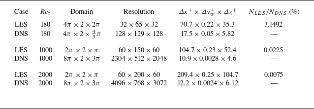
The Reynolds numbers and corresponding resolutions for all simulations are summarised in table 1. All results were gathered within the statistically steady state and compared with the DNS benchmark from Moser et al. (Reference Moser, Kim and Mansour1999) and Lee & Moser (Reference Lee and Moser2015) after adequate time averaging.
Grid resolution (
 $x,y,z$
) for current LES and benchmark DNS (Moser et al. Reference Moser, Kim and Mansour1999; Lee & Moser Reference Lee and Moser2015).

6.1. Recasting of similarity model based on physical space filtering
Following the previous works on homogeneous, isotropic turbulence (Domaradzki Reference Domaradzki2024), the extended ITM is first applied to the test-filtered velocity based on the physical space filtering. While a sharp spectral cutoff filter provides a direct connection between subgrid and subfilter scales, it cannot be used for fully inhomogeneous flows. Therefore, we explore the applicability of the new model with a smooth filter. In this subsection, a Gaussian filter is chosen to compute the test-filtered field,
 \begin{equation} G(x, x') = \sqrt {\frac {\gamma }{\pi \unicode{x1D6E5} ^2}} \exp \left (-\frac {\gamma |x - x'|^2}{\unicode{x1D6E5} ^2} \right )\\ \text{ or, in spectral space, }\quad \widehat {G}(k) = \exp \left (\frac {-\unicode{x1D6E5} ^2 k^2}{4\gamma } \right ), \end{equation}
where a commonly used value of
 $\gamma =6$
is used for all simulations. The filter is smooth in both physical and spectral space. In practice, the Gaussian filter is commonly used to compute the similarity model (Bardina et al. Reference Bardina, Ferziger and Reynolds1980; Piomelli et al. Reference Piomelli, Moin and Ferziger1988), facilitating direct comparisons with our new approach. The similarity model computed from smooth filters also exhibits relatively high correlations in a priori analysis (Liu et al. Reference Liu, Meneveau and Katz1994). For ease of implementation, in this subsection, the filter is applied only to the horizontal directions. Note that the similarity model (4.2) generates an inhomogeneous SGS stress in the vertical direction, so the modelling is still three-dimensional. The model is then converted to the eddy viscosity form following the procedures leading to (4.4) or (4.15). For inhomogeneous flow defined in physical space, it is not straightforward to evaluate the coefficient
 $C$
in (4.15) theoretically. As discussed in (4.14), the Gaussian filter with characteristic filter width
 $\overline {\unicode{x1D6E5} }$
equal to the mesh size
 $\unicode{x1D6E5}$
leads to the desired factor
 ${1}/{12}$
in the equation. Moreover, the connection with the gradient model further supports setting
 $C=1$
for the current filter.
Results for ITM based on the Gaussian filter compared with other SGS models.

(a) Mean velocity profiles and (b) r.m.s. velocities for
 $Re_\tau \approx 1000$
, the ITM is based on the Gaussian filter and 1-D line averaging of the eddy viscosity.

(a) Mean velocity profiles and (b) r.m.s. velocities for
 $Re_\tau \approx 2000$
, the ITM is based on the Gaussian filter.

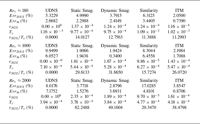
For various Reynolds numbers, the performance of our new model is compared with the no-model simulations and LES with the Smagorinsky models summarised in table 2. Corresponding results are shown in figures 2–4. Specifically, ‘UDNS’ implies the no-model under-resolved DNS runs. The static Smagorinsky denoted as ‘static Smag.’ always adopts a common choice of
 $C_S=0.1$
along with the Van Driest damping function (Van Driest Reference Van Driest1956). The dynamic Smagorinsky model based on the Germano identity (Germano et al. Reference Germano, Piomelli, Moin and Cabot1991) and extended by Lilly (Reference Lilly1992) is used to compute the modelling coefficients and is denoted as ‘dynamic Smag.’, which applies a local averaging and zero-clipping of
 $C_S$
as described in our previous works (Cadieux & Domaradzki Reference Cadieux and Domaradzki2015; Sun & Domaradzki Reference Sun and Domaradzki2018). The SGS dissipation and the viscous transfer
 $T_\nu = -\nu \boldsymbol {u} \nabla ^2 \boldsymbol {u}$
in the table were averaged over the entire channel. For higher Reynolds numbers, the contribution of SGS dissipation for all models is large, indicating the significant under-resolution in the context of DNS. For the relatively low resolutions used in the present study (see also table 1), no-model UDNS runs are incapable of generating satisfactory results. The Smagorinsky models can reproduce low-order statistics accurately for some Reynolds numbers, but in general, the accuracy is not as good as for the interscale model. In particular, our new model focuses on providing an appropriate amount of total SGS dissipation, so that the mean velocity profiles are reproduced more faithfully. However, unlike our previous work for HIT in which the spectral eddy viscosity can be computed directly, in the physical space implementation, less attention is paid to generate a desired distribution of energy transfer in spectral space. Consequently, the overall errors
 $Err_{{DNS}}$
do not show a clear advantage over the Smagorinsky models.
(a) Horizontally averaged SGS dissipation and (b) 1-D streamwise energy spectra for
 $Re_\tau \approx 180$
. The spectra in the upper part of the figure are for locations inside the buffer layer (
 $y^+ \approx 20$
), and the spectra in the lower part are for locations close to the centre (
 $y^+ \approx 180$
). The ITM is based on the Gaussian filter.

The energy dissipation from the present model is further evaluated using the SGS dissipation and 1-D energy spectra, as shown in figures 5–7. Based on results in table 2, overall, the globally averaged SGS dissipation of the new model generated a similar amount of SGS dissipation as the dynamic Smagorinsky model, especially for the higher
 $Re$
. The peak of
 $\varepsilon _{{SGS}}$
predominantly occurs within the buffer layer where the production of turbulent kinetic energy is the largest, resulting in considerably higher dissipation in this region. Nevertheless, note that the vertical distribution of time-averaged SGS dissipations are plotted on a log scale. For relatively large
 $Re$
, the buffer layer constitutes only a small fraction of the channel height. In contrast, the dynamic Smagorinsky model predicts a relatively more uniform distribution of
 $\varepsilon _{{SGS}}$
across the channel, leading to a comparable total SGS dissipation to that of the ITM after vertical integration. For all simulations with the new model, the energy spectra closely follow the DNS benchmark and no non-physical energy accumulation is observed. This indicates that the present model effectively regularises the energy cascade at resolved scales.
(a) Horizontally averaged SGS dissipation and (b) 1-D streamwise energy spectra for
 $Re_\tau \approx 1000$
. The spectra in the upper part of the figure are for locations inside the buffer layer (
 $y^+ \approx 20$
) and the spectra in the lower part are for locations close to the centre (
 $y^+ \approx 1000$
). The ITM is based on the Gaussian filter.

(a) Horizontally averaged SGS dissipation and (b) 1-D streamwise energy spectra for
 $Re_\tau \approx 2000$
. The spectra in the upper part of the figure are for locations inside the buffer layer (
 $y^+ \approx 20$
) and the spectra in the lower part are for locations close to the centre (
 $y^+ \approx 2000$
). The ITM is based on the Gaussian filter.

Instantaneous eddy viscosity at
 $Re_\tau \approx 1000$
,
 $(a)$
the dynamic Smagorinsky model,
 $(b)$
the ITM computed from the Gaussian filter.

Eddy viscosities
 $\nu _t$
at
 $Re_\tau \approx 1000$
averaged in the horizontal directions. The curves represent the time-averaged quantities, with the r.m.s. of
 $\nu _t$
displayed as error bars.

To analyse the direction of energy transfer in more detail, we compare the spatial distributions of instantaneous eddy viscosity at
 $Re_\tau \approx 1000$
for the dynamic Smagorinsky model and the interscale model in figure 8. To compare the two models more unambiguously, the eddy viscosities are computed based on the same snapshot of the velocity field, which is taken from a relatively accurate simulation with the dynamic Smagorinsky model. The distribution of eddy viscosity from the interscale model is more uniform: the majority of
 $\nu _t$
is within
 $[0, \, 2\times 10^{-5}]$
and there are only very few regions with backscatter. By contrast, the dynamic Smagorinsky model, despite being purely dissipative after zero-clipping of
 $C_S$
, displays more substantial spatial variability. It is noteworthy that even though the volume-averaged SGS dissipations between the ITM and the dynamic Smagorinsky model are comparable, their primary objectives differ. For a given SGS model, the dynamic procedure (Germano et al. Reference Germano, Piomelli, Moin and Cabot1991) seeks the best estimate for modelling coefficients, whereas the interscale energy transfer model focuses on reproducing the correct amount of total SGS transfer for resolved scales (Domaradzki Reference Domaradzki2024).
Nevertheless, as one can observe from figure 9, the present model yields positive eddy viscosities after averaging in homogeneous directions, which explains why the method is numerically stable and robust in actual simulations. In addition, all models generate comparable eddy viscosities, consistent with the results for total SGS dissipation reported in table 2. The inverse energy transfer for the interscale model originates from the similarity model, which correlates well with the real SGS stress in a priori analysis (Liu et al. Reference Liu, Meneveau and Katz1994). The allowance of backscatter is inherited from the similarity model, which is one of the key ingredients that differentiates the present model from other models that rarely take negative eddy viscosities into account. The recasting to the eddy viscosity form offers a strategy to provide an appropriate amount of total SGS dissipation while preserving the desired energy transfer distribution of the similarity model, so additional adjustments are not necessary.
Instantaneous SGS dissipation at
 $Re_\tau \approx 1000$
:
 $(a)$
the similarity model;
 $(b)$
ITM. The coloured region shows
 $\varepsilon _{{SGS}} \geqslant 0$
, the white region indicates backscatter.

Furthermore, the effect of recasting to reduce the inverse energy transfer is further evaluated in figure 10, in which the energy dissipation of similarity model before and after reshaping is compared. Due to the relatively wide range of quantities, we only show positive and negative energy dissipation in the plots. In the original similarity model (Bardina et al. Reference Bardina, Ferziger and Reynolds1980), only roughly half of the SGS dissipation is positive, indicating the backscatter is significant. The observation is consistent with previous studies of SGS energy transfer (Piomelli et al. Reference Piomelli, Cabot, Moin and Lee1991; Domaradzki et al. Reference Domaradzki, Liu and Brachet1993). After recasting to the eddy viscosity form, forward energy cascade regions become more dominant. Note that even though large backscatter is expected in fully resolved DNS runs, in LES with relatively low resolutions, the total SGS dissipation is positive and makes notable contribution to the combined effect of small-scale energy removal. In contrast, substantial backscatter from the similarity model can easily destabilise simulations and lead to unsatisfactory results. Therefore, the recasting in the current model can be considered as a simple but effective technique of backscatter control.
6.2. Effect of filter shape
In practice, the Gaussian filter in the previous subsection may not be easy to implement for complex geometries. In this section, we aim to extend the applicability of the model based on various 3-D discrete filtering in physical space. Based on the concept of interscale energy transfer in § 4, the precise filter shape may not be crucial, as long as the correct amount of total SGS dissipation is maintained on the LES grid.
In the current work, we choose a common discrete filter based on a three-point kernel
 \begin{equation} \overline {u}_n {=} G\star u_n {=} \frac {c}{4} u_{n-1} + \!\left (1 - \frac {c}{2} \right ) u_n + \frac {c}{4} u_{n+1}, \text{ where } G(x-x') = \!\!\sum ^{1}_{j=-1} c_j \delta (x - x' + j\unicode{x1D6E5} ), \end{equation}
or equivalently in spectral space,
 \begin{equation} \widehat {G}(k) = 1 - c \sin ^2 \left (k \frac {\unicode{x1D6E5} }{2} \right ). \end{equation}
Furthermore, to create weaker filters within a three-point kernel, we employ a soft deconvolution proposed by van Cittert (Reference van Cittert1931). The method was originally developed for image reconstruction and plays a central role in the family of the approximate deconvolution model (ADM) (Stolz & Adams Reference Stolz and Adams1999). Assuming that
 $G$
is an invertible filter, it is theoretically possible to recover the full velocity field from its filtered version by applying a filter inverse, such that
 $u = G^{-1} \star \overline {u} \approx Q_N \star \overline {u}$
after successive iterations,
 \begin{equation} G^{-1} \approx Q_N = \sum ^N_{\nu =0} (I - G)^\nu = \frac {I-(I-G)^{N+1}}{G}, \end{equation}
where
 $I$
is the identity matrix and
 $N$
is the deconvolution order. The last term becomes smaller as as
 $N$
increases. In other words, the last term diminishes, meaning that a higher deconvolution order
 $N$
brings the filtered
 $\overline {u}_N$
closer to the original
 $u$
, resulting in a weaker filtering operation. Consequently, a secondary filter can be constructed as the product of
 $Q_N$
and
 $G$
:
 \begin{equation} Q_N G = \sum ^N_{\nu =0} (I - G)^\nu G = I-(I-G)^{N+1}. \end{equation}
In this way, the deconvolution-type filter can be constructed as the product of
 $Q_N$
and
 $G$
:
 \begin{equation} \overline {u} = (Q_N G) \star u = \left [\sum ^N_{\nu =0} (I - G)^\nu \right ] G \star u, \end{equation}
or in spectral space,
 \begin{equation} \widehat {Q_N G}(k) = 1 - \left [c \sin ^2\left (k \frac {\unicode{x1D6E5} }{2}\right )\right ]^{N+1} = 1 - \left [c - c\cos \left (k \unicode{x1D6E5} \right )\right ]^{N+1}. \end{equation}
Results for ITM performed with 3-point discrete filtering with different deconvolution orders.

Three-point top-hat filters based on equation with similar characteristic filter width, compared with the Gaussian filter:
 $(a)$
filters with
 $\overline {\unicode{x1D6E5} } = \unicode{x1D6E5}$
based on (6.13);
 $(b)$
filters with
 $\overline {\unicode{x1D6E5} } \approx \unicode{x1D6E5}$
based on (6.15), see also table 3.

In practice, an easy way to implement the filter (Jeanmart & Winckelmans Reference Jeanmart and Winckelmans2007) is by calculating the coefficients of the geometric sequence in (6.7),
 \begin{equation} Q_N G = I-(I-G)^{N+1} = a_1 G + a_2 G^2 + \ldots + a_{N+1} G^{N+1}, \end{equation}
in which the coefficients
 $a_i$
can be calculated recursively, thus the filtering operations can be implemented easily and efficiently also in the physical space. The filtering is applied sequentially in all three dimensions.
In this section, we will investigate if the interscale model based on different filters can generate similar results. As discussed in § 4.2, it is desirable for the filter width to be close to the mesh size
 $\unicode{x1D6E5}$
. Therefore, we adjust the filtering coefficient
 $c$
and the deconvolution order
 $N$
in (6.4) and (6.6) to maintain a similar characteristic filter size. For discrete filters, a common way to define filter width is through the standard deviation (Lund Reference Lund1997; Sagaut Reference Sagaut2006). For the three-point filter in (6.4), the ratio between the characteristic filtering width
 $\overline {\unicode{x1D6E5} }$
and the mesh size
 $\unicode{x1D6E5}$
is
 \begin{equation} \alpha = \overline {\unicode{x1D6E5} } / \unicode{x1D6E5} = \sqrt {12 \int ^{\infty }_{-\infty } x^2 G(x) {\rm d}x} = \sqrt {12 \sum _j j^2 c_j} = \sqrt {6c}, \end{equation}
or equivalently in spectral space,
 \begin{equation} \alpha = \overline {\unicode{x1D6E5} } / \unicode{x1D6E5} = \sqrt {-12 \widehat {G}''(0)} / \unicode{x1D6E5} = \sqrt {-6 c \left [\cos ^2\left (k \frac {\unicode{x1D6E5} }{2} \right ) - \sin ^2\left (k \frac {\unicode{x1D6E5} }{2} \right ) \right ]_{k=0} } = \sqrt {6c}. \end{equation}
Similarly, the characteristic filter width for the secondary filters with deconvolution order
 $N$
is
 \begin{equation} \alpha _N = \sqrt {6(N+1) c^{N+1}}. \end{equation}
Based on the results for Gaussian filtering in the previous subsection, here, we would like to find a set of deconvolution-type discrete filtering with characteristic filtering width equal to
 $\unicode{x1D6E5}$
. For comparison, we show discrete filters with
 $\overline {\unicode{x1D6E5} } = \unicode{x1D6E5}$
, obtained from (6.13), alongside the Gaussian filter in figure 11
 $(a)$
. Apparently, the shapes of these discrete filters differ significantly from the Gaussian filter, indicating that the above formula may not be able to characterise the filter width appropriately for deconvolution-type filters. This discrepancy impacts the model’s performance: the filters in figure 11
 $(a)$
produce notably different amounts of SGS dissipation for the interscale model, so the LES results also vary a lot (not shown).
Results for ITM based on three-point discrete filtering with different deconvolution orders.

In this work, we adopt an alternative approach proposed by Lund (Reference Lund1997) to characterise the filter width based on the second moment of the transfer function,
 \begin{equation} M^2 = \int ^{\pi /\unicode{x1D6E5} }_{0} k^2 G(k) {\rm d}k, \end{equation}
which can be computed analytically for the current filters (6.9). Then, the filter width can be estimated by
 \begin{equation} \alpha = \overline {\unicode{x1D6E5} } / \unicode{x1D6E5} = \left [\frac {\pi ^3}{3 M^2 \unicode{x1D6E5} ^3} \right ]^{\frac {1}{3}}. \end{equation}
Note that the constants in this formula were chosen to predict the correct width in the case of an exact Fourier cutoff. The discrete filters with
 $\overline {\unicode{x1D6E5} } \approx \unicode{x1D6E5}$
are compared with the Gaussian filter in figure 11
 $(b)$
and corresponding characteristic filter widths based on (6.15) are summarised in table 3. Compared with the results in figure 11
 $(a)$
based on the previous approach, the overall effects of energy removal based on (6.15) are more similar to those from the Gaussian filter. Since the interscale model is designed from the perspective of energy transfer, it is expected that different filters with comparable amounts of energy removal can generate similar SGS dissipation. Therefore, following the ITM based on the Gaussian filter in § 6.1, we keep the modelling coefficient
 $C = 1$
for all filters.
(a) Mean velocity profiles and (b) r.m.s. velocities for
 $Re_\tau \approx 180$
, the ITM is based on the 3-D discrete filtering with different deconvolution orders.

(a) Mean velocity profiles and (b) r.m.s. velocities for
 $Re_\tau \approx 1000$
, the ITM is based on the 3-D discrete filtering with different deconvolution orders.

In table 3, we did not restrict the characteristic width to be precisely the mesh size
 $\unicode{x1D6E5}$
. For discrete filters used in this subsection, the characteristic width can only be estimated. Due to the approximate deconvolution, filtering with higher-order deconvolutions primarily removes information near the cutoff wavenumber
 $k_c$
, so the overall energy dissipation for filters with higher
 $N$
is relatively smaller. Therefore, we chose to slightly increase the characteristic filter width when
 $N$
increases. It is also noteworthy that the present study uses a high-order spectral method in the horizontal directions, whose spectral accuracy effectively minimises numerical errors. In practice, when lower-order numerical discretisations are applied, the resolved scales are truncated based on modified wavenumber analysis (Lele Reference Lele1992; Castiglioni et al. Reference Castiglioni, Sun and Domaradzki2019) and the combined effect of test-filter may also be altered. Nevertheless, the current test filter in figure 11
 $(b)$
primarily removes information near the grid cutoff. As discussed in § 4.2, the exact distribution of SGS dissipation near the mesh cutoff is of secondary importance, provided that the energy at high wavenumbers is sufficiently attenuated by the cusp feature of eddy viscosity. In addition, the impact of grid filtering or truncation can be minimal if it is less effective than the test filtering. For instance, in classic compact finite difference schemes of sixth order or higher (Lele Reference Lele1992), moderate wavenumbers remain largely unaffected by grid filtering, meaning that information loss is primarily dictated by the test filter in figure 11
 $(b)$
. Therefore, theoretically, the model should yield similar performance when applied to relatively high-order numerical methods. In the future, we will attempt to refine the estimation of the characteristic filter width for discrete filtering and account for numerical discretisations, with the goal of making general SGS models more self-contained.
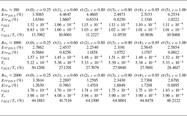
The LES runs of the interscale model based on the discrete filters in table 3 are summarised in table 4and corresponding low-order statistics are shown in figures 12–14. Apparently, for various Reynolds numbers, the SGS dissipation
 $\varepsilon _{{SGS}}$
generated by the ITM with different filtering is close to each other, suggesting that the exact shape of the filter (or the resulting eddy viscosity) is not crucial. When the total SGS dissipations are similar, the overall accuracy of the simulations also does not differ significantly. The results for all filters are relatively satisfactory. In particular, the mean and r.m.s. velocities normally of interest in LES for different filtering almost collapse with each other, underscoring the generality of ITM as an SGS model. Moreover, due to the full 3-D filtering, the model was able to reproduce the DNS benchmark more faithfully, compared with the 2-D Gaussian filtering in the previous subsection.
(a) Mean velocity profiles and (b) r.m.s. velocities for
 $Re_\tau \approx 2000$
, the ITM is based on the 3-D discrete filtering with different deconvolution orders.

(a) Horizontally averaged SGS dissipation and (b) 1-D streamwise energy spectra for
 $Re_\tau \approx 180$
. The spectra in the upper part of the figure are for locations inside the buffer layer (
 $y^+ \approx 20$
) and the spectra in the lower part are for locations close to the centre (
 $y^+ \approx 180$
). The ITM is based on the 3-D discrete filtering with different deconvolution orders.

(a) Horizontally averaged SGS dissipation and (b) 1-D streamwise energy spectra for
 $Re_\tau \approx 1000$
. The spectra in the upper part of the figure are for locations inside the buffer layer (
 $y^+ \approx 20$
) and the spectra in the lower part are for locations close to the centre (
 $y^+ \approx 1000$
). The ITM is based on the 3-D discrete filtering with different deconvolution orders.

(a) Horizontally averaged SGS dissipation and (b) 1-D streamwise energy spectra for
 $Re_\tau \approx 2000$
. The spectra in the upper part of the figure are for locations inside the buffer layer (
 $y^+ \approx 20$
) and the spectra in the lower part are for locations close to the centre (
 $y^+ \approx 2000$
). The ITM is based on the 3-D discrete filtering with different deconvolution orders.

The energy dissipations based on different filtering are further evaluated from the SGS dissipation and 1-D energy spectra in figures 15–17. In general, the zeroth-order filter removes more information at medium scales, leading to relatively high dissipation. Since the non-physical energy pileup due to low grid resolutions mostly occurs near the cutoff wavenumber, in practice, it is generally more advisable to use higher-order filters that minimally affect the large scales. For the relatively high-Reynolds-number cases
 $Re_\tau \approx 1000$
and 2000, the horizontally averaged SGS dissipations from different filters are almost identical, so the overall accuracy of the LES runs is expected to be similar. In addition, by observing the energy spectra, all filters were able to provide sufficient total dissipation and avoid energy accumulation near the LES cutoff
 $k_c$
, suggesting the current procedure is general and not very sensitive to specific implementations.
7. Conclusions
A subgrid scale (SGS) modelling approach based on the interscale energy transfer among resolved scales in LES (Domaradzki Reference Domaradzki2021a ) is extended to inhomogeneous flow. Our primary motivation is to formulate a general modelling procedure by making use of the well-established theoretical foundations of the spectral energy transfer. The approach consists of two main steps, which, in combination, capitalise on the strengths of both structural and functional types of SGS modelling. Following the original idea of reconstructing the total SGS dissipation from a test-filtered field, the subfilter scale stress in physical space is used to obtain the energy dissipation defined on subfiltered scales. The SGS dissipation is then cast in the form of eddy viscosity, with a special focus on preserving the ‘true’ SGS dissipation on the LES mesh. Consequently, the model accomplishes a predominant objective in SGS modelling, which is widely acknowledged to be a necessary condition for accurate LES (Meneveau & Katz Reference Meneveau and Katz2000).
The new model is easy to implement and offers several favourable features. The SGS stress for a test-filtered field is equivalent to the similarity model (Bardina et al. Reference Bardina, Ferziger and Reynolds1983), whose high correlation with the real SGS term helps to maintain a desired distribution of energy transfer. The scale mismatch inherent in the similarity model is corrected during the recasting step, which automatically leads to an effective backscatter control. Unlike typical eddy viscosity models that enforce purely dissipative behaviour, the inverse energy cascade in the present model does not compromise numerical stability and is therefore retained. In addition, the modelling concept does not rely on specific filters. Simple discrete filters with a characteristic width close to the mesh size are capable of consistently generating accurate results. Moreover, the theoretical analyses and satisfactory results for homogeneous, isotropic turbulence (Domaradzki Reference Domaradzki2021a,Reference Domaradzkib) suggest that this model should perform well at high Reynolds numbers. In a posteriori analysis of LES at relatively low resolutions, consistent with the previous studies for isotropic turbulence, the modelling procedure reliably provides an appropriate amount of total SGS dissipation for wall-bounded flow. As a result, the non-physical energy accumulation at small scales is removed, leading to significantly improved low-order turbulent statistics compared with UDNS or LES with the similarity model.
The present study generalises the interscale energy transfer model, but the analysis is limited to channel flow with simple geometry and structured mesh. In the future, we plan to assess the modelling strategy using different numerical methods and attempt to make the model more broadly applicable to complex flow configurations. For unstructured grids, where the discrete filtering method used in this study cannot be directly applied, investigating the effects of scale separation under various test-filtering techniques will be essential. Given the inherently low grid resolution in LES, SGS models should ideally be implemented using high-order numerical schemes to minimise uncertainties arising from the grid filter and the numerical discretisations (Rezaeiravesh et al. Reference Rezaeiravesh, Vinuesa and Schlatter2021). In the finite element method (FEM) framework, various filter transfer functions can be incorporated into local polynomial reconstructions (Blackburn & Schmidt Reference Blackburn and Schmidt2003). Specifically, the test-filtering approach adopted in this study can be applied similarly to the dynamic procedure (Germano et al. Reference Germano, Piomelli, Moin and Cabot1991; Kurz et al. Reference Kurz, Offenhäuser and Beck2023). For lower-order finite volume methods (FVMs), the present approach can still be implemented using differential filters (Lazarov & Sigmund Reference Lazarov and Sigmund2010; Báez Vidal et al. Reference Báez Vidal, Lehmkuhl, Trias and Pérez-Segarra2016) and coarse-graining filters based on face-averaging (Agdestein & Sanderse Reference Agdestein and Sanderse2025). However, the modelling coefficients may require adjustments due to the native numerical dissipation in FVM solvers (Cadieux et al. Reference Cadieux, Sun and Domaradzki2017). In addition, a key challenge in applying spatial filtering to LES is that non-uniform spatial filters do not commute with differentiation, leading to commutation errors and the loss of the divergence-free property in incompressible flows (Ghosal & Moin Reference Ghosal and Moin1995; Langford & Moser Reference Langford and Moser2001). Therefore, we also hope to explore the implementation of the present strategy without test-filtering. Similar to the present study, Qi et al. (Reference Qi, Li, Hu and Yu2022) projected the gradient model onto the eddy viscosity model, employing additional constraints to determine the modelling coefficients instead of relying on test-filtering. The resulting model exhibited high correlations and enhanced scale adaptivity in simulations of various compressible flows. Johnson (Reference Johnson2022) introduced a physics-inspired coarsening (PIC) methodology for LES, which provides a Germano-like dynamic procedure without requiring a test-filter. In PIC, scale separation is achieved through a pseudo-time evolution equation, which has been shown to be mathematically equivalent to Gaussian filtering for unbounded flows on uniform grids, thereby retaining the benefits of spatial filtering. Recently, machine learning techniques have also been used to impose constraints on subgrid scale energy (Novati et al. Reference Novati, de Laroussilhe and Koumoutsakos2021; van Gastelen et al. Reference Van Driest2024). As a future direction, it would be worthwhile to incorporate physical constraints into the LES model via various techniques, further enhancing its adaptability and accuracy across different numerical methods and flow configurations.
Funding.
G.S. is sponsored by the National Natural Science Foundation of China under grants 12272104 and 12402296.
Declaration of interests.
The authors report no conflict of interest.