2 Model and numerical scheme

Figure 1 shows the main features of the axisymmetric computational domain. Liquid flows through a conical region prolonged by a jet and surrounded by a vacuum. The cone jet is enclosed by curves $\unicode[STIX]{x1D6E4}_{1},\unicode[STIX]{x1D6E4}_{2}^{i}$ and $\unicode[STIX]{x1D6E4}_{3}^{i}$ , and the surrounding vacuum by $\unicode[STIX]{x1D6E4}_{1}$ and the circular arc $\unicode[STIX]{x1D6E4}_{2}^{o}$ . The associated surfaces of revolution are termed $\unicode[STIX]{x1D6F4}_{1}$ , $\unicode[STIX]{x1D6F4}_{2}^{i}$ , etc.  $\unicode[STIX]{x1D6E4}_{1}$ is the generatrix of the free surface, $\{x_{o},R_{o}\}$ and $\{x_{f},R_{f}\}$ are its upstream and downstream end points and $\boldsymbol{n}$ and $\boldsymbol{t}$ are its normal and tangential unit vectors. The unknowns of the model are the velocity $\boldsymbol{v}$ , pressure $p$ and the electric potential $\unicode[STIX]{x1D719}^{i}$ fields inside the fluid domain; the electric potential in the vacuum, $\unicode[STIX]{x1D719}^{o}$ ; and the surface charge $\unicode[STIX]{x1D70E}$ and the position of the free surface, $r=R(x)$ . All fields are steady and axisymmetric. The equations of conservation of mass and charge, the Navier–Stokes equations, and Laplace’s equation for the electrical potential describe the electro-hydrodynamics and geometry of the cone jet (Melcher & Taylor Reference Melcher and Taylor1969; Saville Reference Saville1997; Higuera Reference Higuera2003). The following scales for length $r_{c}$ , electric current $I_{c}$ , velocity $v_{c}$ , pressure $p_{c}$ , electric field $E_{c}$ , electric potential $\unicode[STIX]{x1D719}_{c}$ and surface charge $\unicode[STIX]{x1D70E}_{c}$ are used to non-dimensionalize the equations:

Figure 1.

Computational domain.

The $r_{c}$ scale was first proposed by Gañán-Calvo, Dávila & Barrero (Reference Gañán-Calvo, Dávila and Barrero1997) for the radius of the jet, and our model employs it for both the radial and axial directions (Gamero-Castaño 2010). The current emitted by cone jets is known to scale with $I_{c}$ (Fernández de la Mora & Loscertales Reference Fernández de la Mora and Loscertales1994). All other scales follow from these two choices and the goal of making the non-dimensional variables of order one in the cone-to-jet transition region. The resulting non-dimensional equations of conservation of mass and momentum, and Laplace’s equation inside the fluid are:

Note that the symbols used earlier for the dimensional variables denote now their dimensionless counterparts, while dimensional variables will be henceforth topped by a tilde. Laplace’s equation for the potential in the surrounding vacuum is:

and the equations of conservation of charge, balance of stresses (projected on the $\boldsymbol{n}$ and $\boldsymbol{t}$ vectors), the kinematic condition at the surface and the jump of the components of electric field at the fluid–vacuum interface are:

$v_{S}$ stands for the fluid speed at the free surface, $u$ and $v$ are the axial and radial components of the velocity and $\unicode[STIX]{x1D749}$ is the viscous stress tensor. The dimensionless equations include three independent dimensionless numbers, namely the dimensionless flow rate $\unicode[STIX]{x1D6F1}_{Q}=\unicode[STIX]{x1D70C}KQ/(\unicode[STIX]{x1D6FE}\unicode[STIX]{x1D700}_{o})$ , the group $Re=(\unicode[STIX]{x1D70C}\unicode[STIX]{x1D700}_{o}\unicode[STIX]{x1D6FE}^{2}/(\unicode[STIX]{x1D707}^{3}K))^{1/3}$ referred to in the literature as the electrohydrodynamic Reynolds number and the dielectric constant $\unicode[STIX]{x1D700}$ .

The Taylor potential

is used as boundary condition at $\unicode[STIX]{x1D6E4}_{2}^{o}$ , while the upstream and downstream boundaries of the cone jet, $\unicode[STIX]{x1D6E4}_{2}^{i}$ and $\unicode[STIX]{x1D6E4}_{3}^{i}$ , are modelled as equipotential surfaces. $P_{1/2}$ is the Legendre function of the first kind of degree $1/2$ . The $\unicode[STIX]{x1D6F1}_{Q}^{1/4}$ factor results from making the Taylor potential dimensionless with the scales $r_{c}$ and $\unicode[STIX]{x1D719}_{c}$ . The Taylor potential is the field outside an equipotential semi-infinite, hydrostatic cone in which the capillary tension and the electrostatic stress fully balance each other (Taylor Reference Taylor1964). The solution requires a half-angle $\unicode[STIX]{x1D6FC}_{T}$ of $49.29^{\circ }$ for the cone, in good agreement with observations. In experimental cone jets with jet diameters orders of magnitude smaller than the dimensions of the electrodes, the Taylor potential is a good approximation for an extended region far from both the base of the cone and the area where it transitions into a jet. Furthermore its use as the far-field boundary condition eliminates dependencies on the geometry and the potentials of the electrodes. This agrees with the weak dependence of the electrospray current on the emitter potential and geometry observed in experiments, as long as the diameter of the jet is orders of magnitude smaller than that of the emitter.

A spherical velocity profile with net flow rate $Q$ is imposed at the upstream boundary:

Finally, the initial point $\{x_{o},R_{o}\}$ is modelled as a continuation of the static Taylor cone that implicitly exists upstream of the computational domain. This fixes the radius, the slope, the pressure (the electrostatic stress is fully balanced by capillary tension) and the surface charge at this point:

The Navier–Stokes and mass conservation equations are solved in the streamfunction/vorticity formulation. In axisymmetric problems this reduces the system of three coupled equations for the two velocity components and the pressure, to a system of two coupled equation for two unknowns: the streamfunction $\unicode[STIX]{x1D713}$ , and the vorticity $\unicode[STIX]{x1D714}$ , $\unicode[STIX]{x1D714}=\unicode[STIX]{x2202}v/\unicode[STIX]{x2202}x-\unicode[STIX]{x2202}u/\unicode[STIX]{x2202}r$ . Once these two fields are calculated, the two velocity components can be obtained from the streamfunction, $u=(1/r)(\unicode[STIX]{x2202}\unicode[STIX]{x1D713}/\unicode[STIX]{x2202}r)$ , $v=-(1/r)(\unicode[STIX]{x2202}\unicode[STIX]{x1D713}/\unicode[STIX]{x2202}x)$ and the pressure by integrating the momentum equation. The non-dimensional streamfunction and vorticity equations are:

with boundary conditions:

The boundary conditions are associated with the imposed upstream velocity profile ( $r=S_{U}(x)$ defines the curve $\unicode[STIX]{x1D6E4}_{2}^{i}$ ), the kinematic condition at the surface, the axial symmetry of the problem and soft exit conditions. Equation (2.15b ) is derived from (2.7).

Finally, the Navier–Stokes equation is integrated along $\unicode[STIX]{x1D6E4}_{1}$ to obtain the pressure at the surface:

Figure 2 summarizes the algorithm used to solve the system of equations. We combine the equations into three groups referred to as the fluid problem, (2.12), (2.13) and boundary conditions (2.14)–(2.15); the electric problem, (2.3c ), (2.4), (2.5) and boundary conditions (2.8b ), (2.9), (2.12) and equipotential $\unicode[STIX]{x1D6E4}_{2}^{i}$ and $\unicode[STIX]{x1D6E4}_{3}^{i}$ surfaces; and the Young–Laplace equation (2.6) with initial conditions (2.11a ) and (2.11b ). The fluid and electric problems can be solved for a given surface profile $R_{k}(x)$ . The equations are nonlinear and coupled through the $\unicode[STIX]{x1D70E}E_{t}$ and $v_{S}$ terms in (2.15b ) and (2.5), and an iterative scheme is used: we assume a starting surface velocity and solve the electric problem for the given $R_{k}(x)$ ; the resulting $\unicode[STIX]{x1D70E}E_{t}$ stress is used to solve the fluid problem; the surface velocity is then updated. These steps are repeated until the integrals of the square of the residue of (2.12) and (2.13) become smaller than a desired value. Upon convergence of this inner loop, the calculated velocity, pressure and electric fields, and the assumed surface profile $R_{k}(x)$ will not in general fulfil the Young–Laplace equation, and the least-squares weighted residual method is used to generate an improved surface profile $R_{k+1}(x)$ . That is, we minimize the integral:

where (2.18) is evaluated with the solution from iteration $k$ . The weighted residue scheme is implemented with a surface profile discretized into $n$ nodes, $R_{j}$ , and the integral written as a function of the vector $\boldsymbol{X}=\{R_{2},R_{3},\ldots ,R_{n}\}$ for given values of $RHS_{k}(x)$ and the initial conditions $R_{1},R_{1}^{\prime }$ . Differentiating with respect to $R_{2},\ldots ,R_{n}$ yields a system of $n-1$ nonlinear equations $S_{j}(\boldsymbol{X})$ , and the improved profile $R_{k+1}$ is calculated by taking a small step $\unicode[STIX]{x1D6FF}$ in the direction of the first iteration in a Newton–Raphson scheme:

The fluid and electric problems are computed again with the updated surface profile $R_{k+1}$ , and the steps are repeated until (2.17) is smaller than a desired value.

Figure 2.

Algorithm used for solving the system of equations.

Equations (2.3c ) and (2.4) for the electric potentials are solved using the boundary element method (BEM) with linear elements (Bakr Reference Bakr1986). The resulting system of linear algebraic equations is supplemented with those from the discretization of (2.5) using centred finite differences. The electric problem is then solved at once by direct matrix inversion. The partial differential equations (PDEs) of the fluid problem, (2.12) and (2.13), are discretized using centred finite differences in an orthogonal grid (Fletcher Reference Fletcher1988). The grid is built on a generalized curvilinear coordinate $\{\unicode[STIX]{x1D709},\unicode[STIX]{x1D702}\}$ system such that the free surface and the axis are lines of constant $\unicode[STIX]{x1D702}$ , while $\unicode[STIX]{x1D6E4}_{2}^{i}$ and $\unicode[STIX]{x1D6E4}_{3}^{i}$ are lines of constant $\unicode[STIX]{x1D709}$ . The algebraic equations are linearized, and solved iteratively by direct matrix inversion. Figure 3(a) shows a section of the orthogonal grid. Because the fluid domain transitions from a two-dimensional cone to a slender jet, we employ three successive grids with decreasing numbers of nodes in the $\unicode[STIX]{x1D702}$ direction: the grid placed in the cone typically has 20 nodes in the $\unicode[STIX]{x1D702}$ direction, the central grid has 10 nodes and the grid placed in the jet has 4 nodes. The central grid is centred at the maximum of $R^{\prime \prime }(x)$ and has uniform spacing in the axial direction, while the spacing in the cone and jet grids is non-uniform. The streamfunction, vorticity and their derivatives in the $\unicode[STIX]{x1D709}$ direction are required to be continuous at the interface between adjacent grids. Figure 3(b) shows a typical discretization of the boundaries for the boundary element method. 426, 128, 34 and 4 nodes are inserted in $\unicode[STIX]{x1D6E4}_{1}$ , $\unicode[STIX]{x1D6E4}_{2}^{o}$ , $\unicode[STIX]{x1D6E4}_{2}^{i}$ and $\unicode[STIX]{x1D6E4}_{3}^{i}$ respectively. The nodes are distributed uniformly in $\unicode[STIX]{x1D6E4}_{2}^{o}$ , $\unicode[STIX]{x1D6E4}_{2}^{i}$ and $\unicode[STIX]{x1D6E4}_{3}^{i}$ , and have a variable density in $\unicode[STIX]{x1D6E4}_{1}$ : along the surface of the central grid, where the changes in the electric field and surface charge are most intense, we place one BEM node at the position of each grid node, plus five equally spaced nodes in between (i.e. there are six BEM elements between consecutive central grid nodes); upstream and downstream of the central grid we place one BEM node at the position of each grid node, and insert additional nodes near the ends of the central grid so that the length of the BEM elements changes smoothly (see figure 3 c).

Figure 3.

(a) Detail of the orthogonal grid employed in the solution of the streamfunction and vorticity PDEs; (b) BEM discretization; (c) detail of the BEM nodes and the orthogonal grid in the interface between central and jet grids.

3 Results and discussion

The electrospraying conditions investigated include two dielectric constants, 8.91 and 64.9; two values of the Reynolds number for each dielectric constant ( $Re=0.29$ and 1.12 for $\unicode[STIX]{x1D700}=8.91$ , and $Re=0.40$ and 0.74 for $\unicode[STIX]{x1D700}=64.9$ ); and a range of flow rates for each Reynolds number. Gamero-Castaño (Reference Gamero-Castaño2010) has characterized these electrospraying conditions with solutions of the liquids tributyl phosphate ( $\unicode[STIX]{x1D700}=8.91$ ) and propylene carbonate $(\unicode[STIX]{x1D700}=64.9)$ , and these measurements will be used to validate the numerical results. The flow rates simulated coincide with the ranges measured except for tributyl phosphate at $Re=1.12$ , for which the simulations extend the measurements to much lower and higher flow rates (the ratio between the highest and lowest flow rate is 350). In particular, the lowest flow rate for this solution is clearly outside the stable range observed in our experiments, and the numerical solution may correspond to a linearly unstable base state (Gañán-Calvo et al. Reference Gañán-Calvo, López-Herrera, Herrada, Ramos and Montanero2018). A circular arc $\unicode[STIX]{x1D6E4}_{2}^{o}$ with a radius of 144.0 is employed in the simulations of tributyl phosphate, while the radius is 200.5 for propylene carbonate.

Figure 4.

Dimensionless current $I$ and current in nano-amperes as a function of the dimensionless flow rate parameter $\unicode[STIX]{x1D6F1}_{Q}$ , for (a) tributyl phosphate, $\unicode[STIX]{x1D700}=8.91$ ; and (b) propylene carbonate, $\unicode[STIX]{x1D700}=64.9$ . (c) Numerical values plotted in the form suggested by Gañán-Calvo et al. (Reference Gañán-Calvo, López-Herrera, Herrada, Ramos and Montanero2018), $\,\tilde{I} /I_{o}=2.6\unicode[STIX]{x1D6F1}_{Q}^{1/2}$ .

Figures 4(a) and 4(b) show the electric current emitted by the electrospray as a function of the dimensionless flow rate, both in dimensionless form and in nano-amperes. Squares and circles represent experimental and numerical data respectively. The lowest dimensionless flow rates in the experimental series are near the minimum values at which the cone jets were stable. The current in nano-amperes follows the linear law $\tilde{I} (nA)\cong a\unicode[STIX]{x1D6F1}_{Q}^{1/2}+b$ , which in dimensionless form translates to $I\cong (1/I_{o})(a+b\unicode[STIX]{x1D6F1}_{Q}^{-1/2})$ , $I_{o}=(\unicode[STIX]{x1D700}_{0}\unicode[STIX]{x1D6FE}^{2}/\unicode[STIX]{x1D70C})^{1/2}$ . The simulations yield a negative interception $b$ with the ordinate, $-1.96~\text{nA}$ for tributyl phosphate and $-19.7~\text{nA}$ for propylene carbonate. Thus the dimensionless current asymptotes to a constant value at large $\unicode[STIX]{x1D6F1}_{Q}$ , and declines at the lowest $\unicode[STIX]{x1D6F1}_{Q}$ values. The current has a negligible dependence on the Reynolds number, while is a stronger function of the dielectric constant: the asymptotic value of $I$ at large flow rates is 2.5 for tributyl phosphate and 2.1 for propylene carbonate, a difference that is only due to the different dielectric constants. The numerical results compare well with the measurements: they coincide at flow rates near the minimum, and the numerical values become slightly larger at increasing flow rate. This trend occurs in all cases, and is likely due to the decreasing electrification of the experimental cone jets at increasing flow rate, compared to the conditions in the simulations: in the experiments the emitter potential was kept constant at all flow rates, while in the model the Taylor potential varies as $\unicode[STIX]{x1D6F1}_{Q}^{1/4}$ . The reduced electrification in the experiments manifests as a progressive enlargement of the liquid meniscus, which evolves into an expanding acorn-like shape ending in a Taylor cone at increasing flow rate. Although in experimental cone jets the current is a weak function of the emitter potential (we are unaware of any work quantifying this), it does increase with it, which qualitatively coincides with the trend in figure 4(a,b). Finally, figure 4(c) plots the numerical results together, following Gañán-Calvo’s universal scaling law $\tilde{I} /I_{o}=\unicode[STIX]{x1D6FC}\unicode[STIX]{x1D6F1}_{Q}^{1/2}$ . Note that the linear law used in figure 4(a,b) is similar to Gañán-Calvo’s, except for the inclusion of an intercept with the $y$ -axis and a slope that are functions of the dielectric constant. Gañán-Calvo et al. (Reference Gañán-Calvo, López-Herrera, Herrada, Ramos and Montanero2018) show that a massive number of experimental data for a large number of liquids, covering a remarkable $\unicode[STIX]{x1D6F1}_{Q}$ range of over five orders of magnitude, distribute closely to the universal scaling law when the constant $\unicode[STIX]{x1D6FC}$ has a value of 2.6. Although the ability of Gañán-Calvo’s law to approximate the data across such a broad range of dimensionless flow rates is remarkable, it is also apparent in figure 7 of Gañán-Calvo et al. (Reference Gañán-Calvo, López-Herrera, Herrada, Ramos and Montanero2018), as well as in figure 4(c) of this article, that the data for a number of liquids separate to some extent from the universal law. For example, our results for tributyl phosphate at the largest flow rates coincide with Gañán-Calvo’s law (compare the asymptotic value of 2.5 for $I$ , with the slope of 2.6 found by Gañán-Calvo et al.), while the data for propylene carbonate fall below. Our numerical results suggest that the $\tilde{I} /I_{o}=2.6\unicode[STIX]{x1D6F1}_{Q}^{1/2}$ law neglects dependencies on the dielectric constant, and that its accuracy should increase for decreasing $\unicode[STIX]{x1D700}$ and increasing $\unicode[STIX]{x1D6F1}_{Q}$ , i.e. as the surface charge is closer to equilibrium (to be discussed later in the article). This is to be expected because Gañán-Calvo’s law is derived under the assumption of surface charge equilibrium.

Figure 5.

Position of the surface and evolution of the surface and bulk currents in the cone-to-jet transition for: (a) tributyl phosphate at fixed $\unicode[STIX]{x1D6F1}_{Q}$ and two $Re$ ; (b) propylene carbonate at fixed $\unicode[STIX]{x1D6F1}_{Q}$ and two $Re$ ; (c) tributyl phosphate at fixed $Re$ and two $\unicode[STIX]{x1D6F1}_{Q}$ ; (d) propylene carbonate at fixed $Re$ and two $\unicode[STIX]{x1D6F1}_{Q}$ ; and (e) tributyl phosphate and propylene carbonate at fixed $\unicode[STIX]{x1D6F1}_{Q}$ .

Figure 5(a–e) shows the position of the surface, and the evolution of the bulk and surface currents in the axial direction, for a variety of electrospraying conditions. The origin of the abscissa is set at the maximum of $R^{\prime \prime }(x)$ , $x_{R_{max}^{\prime \prime }}$ . The surface and bulk currents, associated with convection of surface charge and electric conduction in the bulk, are given by:

$\unicode[STIX]{x1D6E4}$ is any curve inside the cone jet that starts at the axis and ends at $R(x)$ , e.g. in the calculations we use gridlines of constant $\unicode[STIX]{x1D709}$ . The total current, $=I_{S}(x)+I_{B}(x)$ , is constant due to conservation of charge. Figure 5(a,b) shows the effect of varying $Re$ at constant $\unicode[STIX]{x1D6F1}_{Q}$ and $\unicode[STIX]{x1D700}$ ; $\unicode[STIX]{x1D6F1}_{Q}$ is varied at constant $\unicode[STIX]{x1D700}$ and $Re$ in figure 5(c,d); and figure 5(e) illustrates the dependency on $\unicode[STIX]{x1D700}$ ( $\unicode[STIX]{x1D6F1}_{Q}$ is fixed while the Reynolds number has a small effect). Charge is injected on the surface as the cone transitions into the jet, and the surface current progressively increases at the expense of the bulk current. The cross-over point between the surface and bulk currents is located downstream of $x_{R_{max}^{\prime \prime }}$ . The total current is a weak function of both $Re$ and $\unicode[STIX]{x1D6F1}_{Q}$ for tributyl phosphate, depends slightly on these parameters in propylene carbonate and displays a larger variation with the dielectric constant. The profiles of the cone jets are surprisingly similar despite the wide ranges of $\unicode[STIX]{x1D6F1}_{Q}$ , $Re$ and $\unicode[STIX]{x1D700}$ . The overlap is unexpected because of the presence of these parameters in the model equations, and supports the choice of $r_{c}$ as the characteristic length scale in both the radial and axial directions. Note also that the transition from cone to jet is smoother, i.e. the surface profile has larger radii of curvature in an interval around $x_{R_{max}^{\prime \prime }}$ , at both increasing dimensionless flow rate and decreasing dielectric constant. The overlap of the surface profiles when they are scaled with $r_{c}$ was first discovered by Gamero-Castaño (Reference Gamero-Castaño2010) on the bases of experimental measurements of the energy deficit of electrosprayed droplets; Gamero confirmed the overlap with numerical solutions of profiles computed by Higuera (Reference Higuera2003). Gañán-Calvo et al. (Reference Gañán-Calvo, López-Herrera, Herrada, Ramos and Montanero2018) have also confirmed the overlap using numerical simulations.

Figure 6.

Position of the surface and its second derivative, bulk and surface current, ratio between the surface current and its equilibrium value and normal stresses for (a) propylene carbonate, $\unicode[STIX]{x1D6F1}_{Q}=87.4$ , $Re=0.40$ , and (b) tributyl phosphate, $\unicode[STIX]{x1D6F1}_{Q}=87.4$ , $Re=0.29$ . Equation (2.6) reads $\unicode[STIX]{x1D70F}_{\unicode[STIX]{x1D6FE}}=\unicode[STIX]{x1D70F}_{P}+\unicode[STIX]{x1D70F}_{\unicode[STIX]{x1D707}}+\unicode[STIX]{x1D70F}_{En}+\unicode[STIX]{x1D70F}_{Et}$ in terms of the labels.

Figure 6(a,b) shows the position of the surface and its second derivative, the bulk and surface currents, the ratio between the surface current and the equilibrium surface current and the different stresses in the Young–Laplace equation, for the two dielectric constants and fixed dimensionless flow rate, $\unicode[STIX]{x1D6F1}_{Q}=87.4$ . The Reynolds numbers are not identical, but differences associated with this parameter are small. The equilibrium surface current, $\tilde{I} _{eq}=2\unicode[STIX]{x03C0}\unicode[STIX]{x1D700}_{0}\tilde{R}\tilde{v}_{s}\tilde{E}_{n}^{o}$ , is the limiting value associated with a distribution of charge that fully shields the bulk from the external electric field, i.e. that would make $\tilde{E}_{n}^{i}=0$ or equivalently $\tilde{\unicode[STIX]{x1D70E}}=\unicode[STIX]{x1D700}_{0}\tilde{E}_{n}^{o}$ . Using this definition and the surface convection time $\text{d}t=\sqrt{1+R^{\prime 2}}(\text{d}x/v_{S})$ , the equation of conservation of charge (2.5) can be written in the form:

As a fluid particle moves down the surface the surface current approaches the equilibrium value exponentially, with a time constant given by the ratio between the electric relaxation time $\unicode[STIX]{x1D700}\unicode[STIX]{x1D700}_{0}/K$ and the flow residence time $r_{c}/v_{c}$ . Fernández de la Mora & Loscertales (Reference Fernández de la Mora and Loscertales1994) used this equation to explain the breakdown of Taylor’s solution when applied to an experimental cone jet: they argued that far upstream from the vertex the electric relaxation time is much smaller than the residence time, the surface current adopts its equilibrium value and the electro-hydrostatic Taylor cone solution is valid. However as the fluid approaches the vertex both times become comparable, $I_{S}$ and $I_{eq}$ differ and a significant electric field develops inside the liquid which, by injecting charge onto the surface, attempts to restore equilibrium. On the other hand, Gañán-Calvo (Reference Gañán-Calvo1997, Reference Gañán-Calvo2004) has argued that the position of the free surface is such that $I_{S}$ and $I_{eq}$ are approximately equal everywhere, i.e. that the surface charge is always relaxed or in equilibrium. More recently Gañán-Calvo, Rebollo-Muñoz & Montanero (Reference Gañán-Calvo, Rebollo-Muñoz and Montanero2013) have proposed that for liquids with $\unicode[STIX]{x1D700}Re>1$ , which is the case in this article, the surface charge is not in equilibrium near the minimum flow rate. Figure 6(a,b) shows that the ratio $I_{S}/I_{eq}$ departs significantly from one in the region where the cone transitions into a jet, the deficit being larger for the larger dielectric constant: the minimum value of $I_{S}/I_{eq}$ is 0.62 for $\unicode[STIX]{x1D700}=64.9$ , and 0.92 for $\unicode[STIX]{x1D700}=8.91$ . This is to be expected since at constant $\unicode[STIX]{x1D6F1}_{Q}$ and almost constant geometry (see figure 5 e), the ratio between the electric relaxation and flow residence times is proportional to the dielectric constant. Figures 6(a) and 6(b) also show that, sufficiently upstream of the vertex where the surface charge is in equilibrium ( $I_{S}/I_{eq}\cong 1$ ), the electrostatic stress component $\unicode[STIX]{x1D70F}_{En}$ fully balances the capillary tension $\unicode[STIX]{x1D70F}_{\unicode[STIX]{x1D6FE}}$ in agreement with Taylor’s solution. As $I_{S}/I_{eq}$ decreases the stress component $\unicode[STIX]{x1D70F}_{Et}$ , absent in Taylor’s equipotential cone, becomes important in the balance of normal stresses, and the surface current increases. the value of $\unicode[STIX]{x1D70F}_{Et}$ is proportional to the dielectric constant, and its high value for propylene carbonate makes $\unicode[STIX]{x1D70F}_{Et}$ larger than $\unicode[STIX]{x1D70F}_{En}$ in the transition region of this liquid; furthermore, to balance this large $\unicode[STIX]{x1D70F}_{Et}$ stress pulling the surface, the pressure becomes significant and negative. Downstream, as the $I_{S}/I_{eq}$ ratio returns to one (i.e. the surface charge approaches equilibrium), the surface current asymptotes to the total current, the electric stress asymptotes to a constant or slowly varying value and the balance of stresses is fulfilled by an increasing positive fluid pressure. The normal component of the viscous stress is negligible everywhere. The higher values of $R^{\prime \prime }(x)$ for propylene carbonate indicate that the radius of curvature in an interval a few units around $x_{R_{max}^{\prime \prime }}$ is smaller than for tributyl phosphate, i.e. at constant dimensionless flow rate the transition from cone to jet in propylene carbonate is sharper than in tributyl phosphate.

Figure 7(a,b) shows $I_{S}/I_{eq}$ along the axis at several flow rates, for propylene carbonate ( $Re=0.397$ ) and tributyl phosphate ( $Re=1.12$ ) respectively. Figure 7(c) shows the minimum value of $I_{S}/I_{eq}$ as a function of $\unicode[STIX]{x1D700}/(\unicode[STIX]{x03C0}\unicode[STIX]{x1D6F1}_{Q}^{1/2})$ , for all solutions and flow rates simulated. All flow rates in these figures were reproduced in experiments except for the tributyl phosphate solution with $Re=1.12$ , which was characterized in the range $6.23\leqslant \unicode[STIX]{x1D6F1}_{Q}\leqslant 35.1$ (Gamero-Castaño Reference Gamero-Castaño2010). The lowest flow rate for this solution, $\unicode[STIX]{x1D6F1}_{Q}=1$ , is significantly smaller than the minimum at which it was stable. Consistent with the $\unicode[STIX]{x1D700}/(\unicode[STIX]{x03C0}\unicode[STIX]{x1D6F1}_{Q}^{1/2})$ coefficient in (3.2), the deficit of $I_{S}/I_{eq}$ from one accentuates at increasing dielectric constant and decreasing flow rate. The less polar fluid, tributyl phosphate, exhibits the largest minimum values of $I_{S}/I_{eq}$ : 0.965 for $Re=1.12$ , $\unicode[STIX]{x1D6F1}_{Q}=316.2$ ; and 0.962 for $Re=0.290$ , $\unicode[STIX]{x1D6F1}_{Q}=240.7$ . At these conditions, the surface charge is very near its equilibrium value everywhere along the cone-jet’s surface. On the other hand propylene carbonate, with its large dielectric constant, exhibits the states observed in experiments with smallest values of $I_{S}/I_{eq}$ : 0.421 for $Re=0.74$ , $\unicode[STIX]{x1D6F1}_{Q}=20.0$ ; and 0.560 for $Re=0.397$ , $\unicode[STIX]{x1D6F1}_{Q}=59.3$ . The surface charge along the transition region under these conditions is far from equilibrium. Between these two extreme cases, the shortfall of the surface charge from equilibrium is primarily governed by the value of $\unicode[STIX]{x1D700}/(\unicode[STIX]{x03C0}\unicode[STIX]{x1D6F1}_{Q}^{1/2})$ .

Figure 7.

Ratio between the surface current and its equilibrium value as a function of axial position and at several flow rates for (a) propylene carbonate and $Re=0.397$ , and (b) tributyl phosphate and $Re=1.12$ . (c) Minimum value of the $I_{S}/I_{eq}$ ratio versus $\unicode[STIX]{x1D700}/(\unicode[STIX]{x03C0}\unicode[STIX]{x1D6F1}_{Q}^{1/2})$ , for tributyl phosphate ( $\unicode[STIX]{x1D700}=8.91$ ) and propylene carbonate ( $\unicode[STIX]{x1D700}=64.9$ ).

Figure 8 shows the radius of the cone jet at two significant axial positions: at the current cross-over, $R_{X}$ ; and at the point where the ratio $I_{S}/I_{eq}$ falls by 10 % of its maximum drop, $R_{B}$ . The latter is a reference point for the breakdown of Taylor’s solution. $R_{X}$ depends very slightly on the dielectric constant, while $R_{B}$ increases moderately with $\unicode[STIX]{x1D700}$ . Both radii are insensitive to the Reynolds number. They are also insensitive to variations of the flow rate in the range in which the cone jet is stable, while both radii increase at decreasing $\unicode[STIX]{x1D6F1}_{Q}$ for the two lowest flow rates of the $\unicode[STIX]{x1D700}=8.91$ , $Re=1.12$ case. These two lower flow rates are below the minimum observed in experiments. Thus, the scale $r_{c}$ is not only the correct characteristic radial length throughout the transition region, but when the radius of the surface is expressed in $r_{c}$ units, its value at significant axial points depends very slightly on the dimensionless numbers parametrizing the solution. Note that, although $R_{B}$ is defined at the onset of charge relaxation effects, the radius of the surface in this region scales with $r_{c}$ instead of $r_{FM}$ . This suggests that the coupling between the different variables throughout the transition region may reduce the validity of the local balance used by Fernández de la Mora & Loscertales (Reference Fernández de la Mora and Loscertales1994) to derive the characteristic length $r_{FM}$ .

Figure 8.

Radius of the cone jet at the current cross-over, and typical value in the area where surface charge equilibrium breaks down, as a function of the dimensionless flow rate.

Figure 9 shows the axial extent $L$ of the transition region as a function of the dimensionless flow rate. $L$ is defined as the length of the interval where the surface current changes from 5 % to 95 % of its final value. While the dependency on the Reynolds number is insignificant, the dielectric constant has a strong effect on the value of $L$ . At constant $\unicode[STIX]{x1D6F1}_{Q}$ and increasing $\unicode[STIX]{x1D700}$ , the larger ratio between the electric relaxation and the flow residence times slows down the merging of the surface current with its equilibrium value, and a longer transition region is needed to equilibrate the surface charge. $L$ is a relatively weak function of $\unicode[STIX]{x1D6F1}_{Q}$ : a power fit yields $L\sim \unicode[STIX]{x1D6F1}_{Q}^{0.09}$ for propylene carbonate, and $L\sim \unicode[STIX]{x1D6F1}_{Q}^{0.17}$ for tributyl phosphate. This indicates that $r_{c}$ is a good scale for the axial extent $L$ of the transition region and, being also the characteristic length in the radial direction, the shape of the transition region scaled with $r_{c}$ , is relatively invariant to changes of $\unicode[STIX]{x1D6F1}_{Q}$ and $Re$ . Since these dimensionless numbers are present in the model equations and parametrize the solutions, the near invariant shape of the transition region is a surprising fact. The large values that $\unicode[STIX]{x1D6F1}_{Q}$ adopts in typical electrospraying conditions may contribute to this unexpected property.

Figure 9.

Length of the transition region as a function of the dimensionless flow rate.

Figure 10(a,b) shows the maximum values of the normal and tangential components of the outer electric field at the surface of the cone jet. The maxima are located slightly downstream of the current cross-over. The electric field decreases slightly at increasing dielectric constant, and is a very weak function of the Reynolds number. A power fit of the tangential component yields $E_{t,max}\sim \unicode[STIX]{x1D6F1}_{Q}^{0.06}$ for propylene carbonate, and $E_{t,max}\sim \unicode[STIX]{x1D6F1}_{Q}^{0.09}$ for tributyl phosphate. This weak dependence is to be expected from the definition of the $E_{c}$ scale, which is based on the characteristic tangential component in the transition region:

since both $I$ and $R_{X}$ are weak functions of the dimensionless flow rate, $E_{t,max}$ must also be a weak function of $\unicode[STIX]{x1D6F1}_{Q}$ . The normal component scales as $E_{n,max}^{o}\sim \unicode[STIX]{x1D6F1}_{Q}^{0.48}$ for propylene carbonate and $E_{n,max}^{o}\sim \unicode[STIX]{x1D6F1}_{Q}^{0.44}$ for tributyl phosphate, i.e. nearly as the square root of the dimensionless flow rate. This dependence is also to be expected because at the current cross-over the surface current equals the bulk conduction current, and the surface charge is of the order of $\unicode[STIX]{x1D700}_{0}E_{n}^{o}$ :

Gañán-Calvo (Reference Gañán-Calvo2004) originally put forward the same arguments to establish the scaling of $\tilde{E}_{t,max}$ and $\tilde{E}_{n,max}^{o}$ . On the other hand, he argues for a scaling for the axial length, $\tilde{L}_{G-C}\sim \unicode[STIX]{x1D6FE}/(\unicode[STIX]{x1D700}_{0}\tilde{E}_{t}^{2})\sim (\unicode[STIX]{x1D700}_{0}^{2}\unicode[STIX]{x1D6FE}/\unicode[STIX]{x1D70C}K^{2})^{1/3}\unicode[STIX]{x1D6F1}_{Q}$ , which is different from the scaling observed in figure 9, $\tilde{L}=f(\unicode[STIX]{x1D700})(\unicode[STIX]{x1D700}_{0}^{2}\unicode[STIX]{x1D6FE}/\unicode[STIX]{x1D70C}K^{2})^{1/3}\unicode[STIX]{x1D6F1}_{Q}^{(1/2)+\unicode[STIX]{x1D6FD}}$ , with $\unicode[STIX]{x1D6FD}$ equal to 0.09 and 0.17 for propylene carbonate and tributyl phosphate respectively, i.e. values significantly smaller than the $1/2$ required to match Gañán-Calvo’s scaling.

Figure 10.

Maximum values of the normal (a) and tangential (b) components of the electric field at the surface of the cone jet, on the vacuum side.

The voltage source connected to the emitter injects electric power in the cone jet, which is converted into jet kinetic energy, ohmic and viscous dissipation, surface energy, etc. This balance is important to understanding the physics of electrospraying, e.g. Gañán-Calvo & Montanero (Reference Gañán-Calvo and Montanero2009) use a simplified energy balance to derive the $r_{c}$ scale (the authors assume that the electric power injected within the transition region is mostly transformed into jet kinetic power). The following balance can be derived by integrating the equation of mechanical energy over a volume $\unicode[STIX]{x1D6F1}_{x}$ like the one in figure 1 bounded by surfaces $\unicode[STIX]{x1D6F4}_{2}^{i}$ , $\unicode[STIX]{x1D6F4}_{1}$ , and a surface $\unicode[STIX]{x1D6F4}_{x}$ that intersects $\unicode[STIX]{x1D6F4}_{1}$ downstream at $\{x,r=R(x)\}$ :

Figure 11.

Macroscopic energy balance in the cone jet up to a given axial position. In terms of the labels, equation (3.5) reads $I\unicode[STIX]{x0394}\unicode[STIX]{x1D719}=P_{\unicode[STIX]{x1D6FA}}+P_{\unicode[STIX]{x1D707}}+P_{v}+P_{p}+P_{\unicode[STIX]{x1D749}}$ . Panels (a) and (b) are for tributyl phosphate at $Re=0.29$ and propylene carbonate at $Re=0.397$ , at fixed flow rate $\unicode[STIX]{x1D6F1}_{Q}=87.4$ .

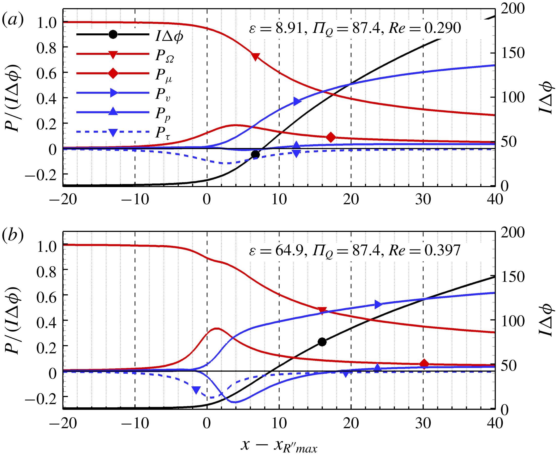
The left-hand side is the electric power supplied to $\unicode[STIX]{x1D6F1}_{x}$ . When $\unicode[STIX]{x1D6F4}_{x}$ is an equipotential surface (e.g. a plane perpendicular to the axis placed sufficiently downstream), this term adopts the more obvious form $\tilde{I} [\tilde{\unicode[STIX]{x1D719}}_{S}(x_{o})-\tilde{\unicode[STIX]{x1D719}}_{S}(x)]$ . The first and second terms on the right-hand side are the ohmic, $\tilde{P}_{\unicode[STIX]{x1D6FA}}=\int _{\unicode[STIX]{x1D6F1}_{x}}(\tilde{\boldsymbol{E}}\boldsymbol{\cdot }K\tilde{\boldsymbol{E}})\,\text{d}\tilde{V}$ , and viscous dissipations, $\tilde{P}_{\unicode[STIX]{x1D707}}=\int _{\unicode[STIX]{x1D6F1}_{x}}(\tilde{\unicode[STIX]{x1D749}}\boldsymbol{ : }\unicode[STIX]{x1D735}\tilde{\boldsymbol{v}})\,\text{d}\tilde{V}$ . The kinetic energy density, pressure and viscous stress are negligible far upstream at $\unicode[STIX]{x1D6E4}_{2}^{i}$ , and can be omitted. Figure 11 shows the electric power in $I_{C}\unicode[STIX]{x1D719}_{c}$ units as a function of the axial coordinate, and the terms on the right-hand side divided by the electric power. The electrospraying parameters are the same as in figures 6 and 5(e). The integrals in (3.5) are computed on $\unicode[STIX]{x1D6F4}_{x}$ surfaces defined by lines of constant $\unicode[STIX]{x1D709}$ , see figure 3. Early in the transition region, e.g. at $x-x_{R_{max}^{\prime \prime }}=0$ , the electric power is mostly converted into ohmic dissipation, 94 % for $\unicode[STIX]{x1D700}=8.91$ and 89 % for $\unicode[STIX]{x1D700}=64.9$ (we will continue listing values for the two dielectric constant cases in this order), and viscous dissipation, 12 % and 29 %; the conversion into jet kinetic energy is small, 1 % and 5 %. The sum of the three terms exceed 100 % because the viscous stress flow power at this point is a relatively large and negative, $-9\,\%$ and $-19\,\%$ (the viscous stress is doing work on the fluid), while the values of the pressure flow power are 1 % and $-4\,\%$ . Dissipation still accounts for most of the electric power at the current cross-over ( $x-x_{R_{max}^{\prime \prime }}=6.2$ and 6.1), with combined values of 92 % and 91 %; at this point the values of jet kinetic power are 17 % and 33 %. As the fluid moves further downstream and the current increasingly becomes surface current, the conversion of electric energy into kinetic energy is more efficient. For example, at the point where the surface current reaches 95 % of its final value, $x-x_{R_{max}^{\prime \prime }}=31.8$ and 68.1, the conversion into kinetic energy is 61 % and 70 %, while the combined dissipation is 36 % and 27 % (the balance is completed by a small positive value of the pressure flow power). The profiles of the jet kinetic power are different for the two liquids, having an earlier and steeper increase for propylene carbonate associated with the simultaneous negative pressure flow power: as seen in figure 6, propylene carbonate exhibits a large negative pressure peak around the current cross-over, induced by the large $(\unicode[STIX]{x1D700}-1)\unicode[STIX]{x1D700}_{0}\tilde{E}_{t}^{2}$ normal pulling stress. This pressure profile accelerates the fluid up to the pressure minimum, and slows it down thereafter. The earlier rise of the jet kinetic power requires, from mass conservation, a smaller cone-jet radius in the initial section of the transition region. This is indeed observed in figure 5(e), where the surface of propylene carbonate falls below that of tributyl phosphate, and exhibits a sharper transition from cone to jet; the sharper transition, or smaller radii of curvature, is more evidently inferred from the higher values of $R^{\prime \prime }(x)$ in figure 6(a). A similar sharper transition occurs in figure 5(c,d) at decreasing flow rate for fixed dielectric constant. The correlation of the sharpness of the transition with flow rate and dielectric constant is due to the varying intensity of charge relaxation, as given by the ratio $\unicode[STIX]{x1D700}/\unicode[STIX]{x1D6F1}_{Q}^{1/2}$ in (3.2). When $\unicode[STIX]{x1D700}/\unicode[STIX]{x1D6F1}_{Q}^{1/2}$ is large, the surface current can be significantly smaller than its equilibrium value, and the surface will remain closer to the ideal conical shape farther towards the axis; on the other hand when $\unicode[STIX]{x1D700}/\unicode[STIX]{x1D6F1}_{Q}^{1/2}$ is small, the surface charge approaches equilibrium earlier in the transition region, which is only possible if the surface separates upward from the electrostatic conical shape.

Figure 12.

Ratio between jet kinetic and electric powers, computed in a macroscopic energy balance extended up to the current cross-over axial location, the point where the surface current reaches 95 % of its final value, and 100 units downstream from $x_{R_{max}^{\prime \prime }}$ .

Figure 12 shows the ratio between jet kinetic and electric powers as a function of the dimensionless flow rate, at three axial locations: the current cross-over, the point where the surface current is 95 % of its final value and 100 units downstream from $x_{R_{max}^{\prime \prime }}$ . At the current cross-over, i.e. at approximately the midsection of the transition region, as little as 9 % of the electric power is converted into jet kinetic power for tributyl phosphate near the minimum flow rate, and 26 % at the largest flow rate investigated; the fraction is larger for propylene carbonate, approximately 35 %, due to the acceleration of the flow by the negative pressure peak. Towards the end of the transition region the transitory effect of the negative pressure profile of propylene carbonate has disappeared and the conversion, with values between 54 % and 65 % depending on the flow rate, is similar for both liquids. The balance is dissipated. The power dissipated increases very slightly further downstream (the bulk current is small while viscous dissipation is only significant early in the transition region around the maximum of $R^{\prime \prime }(x)$ ), most of the electric power injected in this downstream region is converted into kinetic energy, and the ratio increases monotonically. The conversion into kinetic energy never reaches 100 % due to the fraction of the electrical power that is dissipated mostly within the transition region. As mentioned above, in order to derive the $r_{c}$ scale Gañán-Calvo & Montanero (Reference Gañán-Calvo and Montanero2009) assume that the electric power injected within the transition region is mostly transformed into jet kinetic power. Although it is not clear at which point of the transition region this balance should be approximately fulfilled, we think that the current cross-over point is the correct location because the derivation also assumes a total current that is of the order of the conduction current. Although the conversion into kinetic energy at the cross-over is relatively small, especially for tributyl phosphate, we think that the argument by Gañán-Calvo and Montanero remains valid because the jet’s kinetic power is in any case of the order of the electric power.