2.1. Camera configurations

A considerable corpus of research has been accumulated within the realm of visual SLAM utilizing monocular, stereo, or RGB-D cameras. Notable examples include MonoSLAM [Reference Davison, Reid, Molton and Stasse5], PTAM [Reference Klein and Murray6], LSD-SLAM [Reference Engel, Schöps and Cremers7], DSO [Reference Engel, Koltun and Cremers8], ORB-SLAM [Reference Mur-Artal, Montiel and Tardos17], ORB-SLAM2 [Reference Mur-Artal and Tardós9], ORB-SLAM3 [Reference Campos, Elvira, Rodriguez, Montiel and Tardos18], and stereo LSD-SLAM [Reference Engel, Stückler and Cremers19]. The SLAM systems that utilize the aforementioned camera configurations have a relatively narrow FoV. This characteristic leads to frequent tracking failures under extreme conditions, including nighttime scenarios, low-texture scenes, dynamic occlusions, dense vegetation, and rapid rotations. To achieve a wider FoV, researchers have begun to adopt monocular panoramic cameras as data input sources. Wang et al. proposed PAL-SLAM, which uses a catadioptric panoramic camera [Reference Wang, Wang, Tian, Hu and Xu20]. Caruso et al. extended the LSD-SLAM to a generic panoramic camera model [Reference Caruso, Engel and Cremers21] and presented an example of using fisheye cameras in SLAM. PAN-SLAM, proposed by Ji et al., introduced a new panoramic camera model for a multiple fisheye camera rig.

The requirement that all cameras in monocular panoramic SLAM systems must be centrally arranged limits the installation flexibility and cannot fully utilize the overlapping FoV between cameras to recover scale information. Therefore, multi-camera SLAM system has attracted extensive research interest. Castle et al. utilized multiple cameras in their SLAM system, but each camera operated independently as a single camera [Reference Castle, Klein and Murray22]. MC-PTAM independently tracks each camera and optimizes the pose of the entire system by using the measurements from all cameras [Reference Harmat, Sharf and Trentini23]. In MultiCo-SLAM [Reference Urban and Hinz24], the stereo information in the overlapping FoV between adjacent cameras was used to initialize the map with the real environmental scale. However, the stereo information is no longer used after map initialization. ROVO [Reference Seok and Lim25] uses four cameras equipped with fisheye lenses as two pairs of stereo facing forward and backward to maximize the stability and accuracy of the pose estimation. Li et al. [Reference Li, Zou and Yu26] enhanced the initialization stability of multi-camera SLAM systems under conditions of limited overlapping FoV and inaccurate extrinsic calibrations. In ref. [Reference Kuo, Muglikar, Zhang and Scaramuzza27], an adaptive initialization scheme was proposed for arbitrary multi-camera SLAM systems. The adoption of arbitrary multi-camera rigs enhances the flexibility and stability of SLAM systems. However, current multi-camera SLAM systems still rely on traditional feature extraction approaches, which leads to insufficient robustness in challenging scenarios.

2.2. Feature extraction methods

In feature-based methods, the extraction of robust features is critical to the stability of visual SLAM systems. Early visual SLAM systems usually relied on hand-crafted features. Tardif et al. [Reference Tardif, Pavlidis and Daniilidis28] used SIFT to extract features from the omnidirectional camera. Kaess and Dellaert used Harris corner detector to identity features from a Multi-camera Rig [Reference Kaess and Dellaert12]. The FAST feature was employed in PTAM [Reference Klein and Murray6], while ORB-SLAM [Reference Mur-Artal, Montiel and Tardos17] utilized ORB features, which are a combination of FAST keypoints and BRIEF descriptors. These hand-crafted features are computationally efficient and perform well in many scenarios. To date, a multitude of SLAM systems, with multi-camera SLAM systems in particular, remain reliant on ORB features as their dominant feature extraction method, such as those proposed in ref. [Reference Yang, Tang, Wang, Song, Wang and Fu29], MultiCol-SLAM [Reference Urban and Hinz24], and MCSLAM [Reference Kaveti, Vaidyanathan, Thamilchelvan and Singh30]. However, the hand-crafted features often struggle in challenging environments [Reference Liu and Aitken15].

With the advancement of deep learning, such techniques have increasingly been incorporated into SLAM systems, for example, in neural visual SLAM [Reference Liu and Deng31] and semantic visual SLAM for dynamic environments [Reference Zhang, Dong, Guo, Ye, Gao, Xiang, Chen and Wu32]. Meanwhile, learned features have emerged as a promising alternative to hand-crafted features. Deep learning-based feature extraction methods, such as LIFT [Reference Yi, Trulls, Lepetit and Fua13], SuperPoint [Reference DeTone, Malisiewicz and Rabinovich14], and HF-Net [Reference Sarlin, Cadena, Siegwart and Dymczyk33], have demonstrated superior performance in terms of robustness and repeatability. In light of the aforementioned advancements, researchers have integrated deep learning paradigms into SLAM systems. Zhang et al. employed the SuperPoint network as the feature extraction module to detect features from monocular or stereo cameras; however, they still adopted a vocabulary-based approach for loop closure detection [Reference Zhang, Dong, Zhang, Zhu, Li and Deng16]. Similarly, works that adopt deep learning approaches to extract features from monocular or stereo inputs also encompasses GCN-SLAM [Reference Tang, Ericson, Folkesson and Jensfelt34], LIFT-SLAM [Reference Bruno and Colombini35], HFNet-SLAM [Reference Liu and Aitken15], and DX-SLAM [Reference Li, Shi, Long, Liu, Yang, Wang, Wei and Qiao36].

In the context of multi-camera SLAM systems, the choice of feature extraction method is even more critical due to the increased complexity of the system. Traditional methods like ORB may not fully exploit the potential of multi-camera rigs, while deep learning-based methods can provide richer and more discriminative features, enhancing the overall system performance.

4.1. Management of arbitrary multi-camera

In the proposed DAMC-SLAM system, a multi-camera data structure is employed for camera management. Specifically, the intrinsic parameters, extrinsic parameters of each individual camera, as well as the overlapping regions among different cameras are loaded by reading the configuration file. Notably, both the number of cameras and the number of overlapping regions support flexible configuration as required. We define the body coordinate system to associate the data from each camera. Figure 2 shows the transformation relationship between coordinate systems. The process of projecting a 3D point onto the image plane of camera $i$ can be modeled as

(1) \begin{equation} \lambda \mathbf{P}_{i}^{'}=K_{i}(\mathbf{T}_{ib}\mathbf{T}_{bw}\mathbf{P}_{w}). \end{equation}

In this equation, $\mathbf{P}_w$ is a 3D point represented in world coordinate system, $K_i$ is the project function of camera $i$ , and $\mathbf{P}_i^{'}$ is the corresponding 2D point in pixel coordinate system of camera $i$ . The transformation matrix $\mathbf{T}_{ib}$ can be obtained by pre-calibration. $\mathbf{T}_{bw}$ is the multi-camera pose that needs to be solved in the SLAM system. DAMC-SLAM supports both fisheye and pinhole camera models. For fisheye cameras, $K_i(\!\cdot\! )$ is instantiated using the radially symmetric model proposed by Kannala and Brandt [Reference Kannala and Brandt37] instead of the full model. This approach helps to reduce computational overhead and enhance system efficiency. The Kannala–Brandt projection function can be written as

(2) \begin{equation} \begin{gathered} r = \theta + k_1\theta ^{3} + k_2\theta ^{5} + k_3\theta ^{7} + k_4\theta ^{9}, \\ u = f_xr cos(\phi ) + c_x , \\ v = f_yrsin(\phi ) + c_y . \end{gathered} \end{equation}

In Eq. (2), $\theta$ and $\phi$ are, respectively, the zenith and horizontal angle of the incoming ray. $k_i$ where $i=1,2,3,4$ and $f_x, f_y, c_x, c_y$ are the intrinsic parameters and can be obtained through pre-calibration.

Figure 2.

Transformation relationship between coordinate systems. $\mathbf{T_{bw}}$ represents the transformation matrix from world coordinate system to body coordinate system. $\mathbf{ T_{ib}}$ and $\mathbf{ T_{jb}}$ represent the transformation matrices from the body coordinate system to the coordinate systems of camera $i$ and $j$ , respectively. $\mathbf{P_1}$ and $\mathbf{ P_2}$ are 3D points, and $\mathbf{ P_{1}^{'}}$ and $\mathbf{ P_{2}^{'}}$ are corresponding 2D points in pixel coordinate systems.

For pinhole cameras, DAMC-SLAM employs a radial–tangential distortion model. Given the normalized coordinates $(x,y)$ , the distorted coordinates and pixel coordinates are computed as

(3) \begin{equation} \begin{gathered} r^2=x^2+y^2, \\ x_d=x(1+k_1r^2+k_2r^4)+2p_1xy+p_2(r^2+2x^2), \\ y_d=y(1+k_1r^2+k_2r^4)+p_1(r^2+2y^2)+2p_2xy, \\ u=f_xx_d+c_x, \quad v=f_yy_d+c_y . \end{gathered} \end{equation}

Here, $k_1$ and $k_2$ are radial distortion coefficients, while $p_1$ and $p_2$ are tangential distortion coefficients. For each camera, the corresponding projection and back-projection functions are configured from its calibration parameters; therefore, the remaining modules can operate with either camera model without modification.

4.2. Tracking

4.2.2. Hybrid initialization

In an arbitrary multi-camera system, the creation of map points can be categorized into two types. As illustrated in Figure 3, for map points located within the overlapping FoV of multi-camera system (e.g., $\mathbf{P}_1$ and $\mathbf{P}_2$ ), their 3D coordinates can be reconstructed via stereo triangulation. For map points that do not lie within such overlapping regions (e.g., $\mathbf{P}_3$ ), initialization can be achieved using structure from motion (SfM) method based on consecutive observations across two multi-frames.

Figure 3.

Illustration of new map point creation. $o$ represents the centers of camera. The arrows indicate the orientation of cameras, while the dashed lines on both sides represent the cameras’ FoV. $\mathbf{P}$ represents new map points that need to be created. $\mathbf{P}_1$ and $\mathbf{P}_2$ are created in one multiframe, respectively, and $\mathbf{P}_3$ is triangulated through two different multi-frames. $\mathbf{T}_{(t-1)t}$ is the transformation matrix from the multi-camera system’s body coordinate at time $t$ to that at time $t-1$ .

Figure 4.

Pipeline of hybrid initialization.

Figure 4. Long description

The flowchart depicts the pipeline of hybrid initialization in visual SLAM systems. It starts with a multi-frame input. The left side of the flowchart shows the stereo initialization process, which includes matching, epipolar check, triangulation, depth check, and a decision point where if the number of points (N) is greater than 200, the map is inserted. If not, the process loops back. The right side of the flowchart shows the mono initialization with stereo information. It begins with a decision point to check if it is the first multi-frame. If yes, it initializes structure from motion (SfM). If no, it proceeds with matching between multi-frames, SfM for each camera, triangulation for other cameras, stereo information insert, and finally, the map is inserted.

To accommodate arbitrary camera configurations, including monocular cameras, multi-camera with non-overlapping FoV, and multi-camera with overlapping FoV, a hybrid initialization method is proposed in this paper. The pipeline of the hybrid initialization is illustrated in Figure 4.

When the system receives the initial multi-frame, the hybrid initialization module first performs stereo initialization. To improve efficiency, KNN matching is limited to features in the predefined overlapping regions specified in the configuration file. After a matched feature pair passes the epipolar constraint check, triangulation is performed according to $s_i\mathbf{x}_j^{\wedge }\mathbf{T}_{ji}\mathbf{x}_i=0$ , where $s_i$ is the depth in camera $i$ . $\mathbf{x}_i$ and $\mathbf{x}_j$ are the coordinates of the same 3D map point on the unit image planes of cameras $i$ and $j$ , respectively, obtained by applying the corresponding camera back-projection functions $K^{-1}(\!\cdot \!)$ . The transformation $\mathbf{T}_{ji}$ is calculated as $T_{ji}=T_{jb}T_{ib}^{-1}$ from the pre-calibrated extrinsic parameters. Thus, $s_i$ is the only unknown and can be solved directly. Map points that pass the depth and reprojection-error checks in both cameras are successfully triangulated. To accelerate the triangulation speed, the computations for different overlapping regions are performed in separate threads. For each triangulated map point, we store its depth and parallax angle for subsequent map point creation in the local mapping module. If more than 200 map points are triangulated, they are inserted into the map. The first multi-frame is designated as a multi-keyframe, and its pose is set to the world coordinate system. Due to the use of stereo information, the real scale of the environment was introduced into the map.

Stereo initialization often fails when cameras have no overlapping FoVs or when too few feature points are available in the overlapping regions. This can occur with a limited number of cameras, small overlapping FoVs, or low-texture regions. In such cases, the hybrid initialization module matches features between two multi-frames and estimates the motion of each camera using SfM. After successful motion estimation, triangulation is applied not only to features in the current camera but also to features from the other cameras. This significantly increases the number of map points generated during initialization and improves system stability. Finally, triple-observation map points are identified from the two multi-frames and added to the map. A triple-observation map point is defined as a point that is observed twice within one multi-frame and at least once in another multi-frame, such as $\mathbf{P}_1$ in Figure 3. Through this mechanism, scale information is inserted into the map. The underlying principle is that two observations within one multi-frame enable the determination of its true coordinates with scale information; meanwhile, the observation in another multi-frame allows for the estimation of the actual motion distance of the multi-camera system.

4.2.3. Pose prediction and tracking in local map

We employ a constant-velocity motion model to predict the pose of the current multi-frame based on the pose of the previous multi-frame. Leveraging the predicted pose, the points in the map are projected onto the current multi-frame in accordance with Eq. (1), followed by a search for matching feature points within the adjacent region. In a multi-camera system, due to the distinct orientations of individual cameras, the displacement distances of feature points across different directions in the image vary significantly. Specifically, feature points where the connection line between the map points and the body coordinate system is parallel to the motion direction exhibit the minimum displacement distance, whereas those with the connection line perpendicular to the motion direction demonstrate the maximum displacement distance. Based on this observation, we assign a unique search distance to each map point individually, which is determined by the angle between the connection line and the motion direction. The calculation of this search distance follows the formula:

(4) \begin{equation} r=\big ( 2-\big |cos(\overrightarrow {bp}, \overrightarrow {v})\big | \big )r_{pre}, \end{equation}

where $\overrightarrow {bp}$ denotes the vector from the body coordinate system of the multi-camera system to a map point, $\overrightarrow {v}$ represents the velocity vector, and $r_{pre}$ stands for the preset search distance.

At the final stage of feature matching, feature points associated with potential dynamic objects are filtered using the segmentation masks to reduce their interference with pose optimization. Not all such feature points are removed. When the semantic mask associated with a potential dynamic label occupies only a small proportion of the image, it contains relatively few feature points and has little effect on pose optimization. In addition, stationary objects, such as parked vehicles, can provide useful features for tracking. In contrast, a large semantic mask associated with a moving object can substantially degrade pose optimization or even cause tracking failure. We therefore compute the area of the semantic mask associated with each potential dynamic label relative to the whole image. Only those feature points associated with masks whose area exceeds a predefined threshold are removed. Based on empirical observations, this threshold is set to one-sixth of the image area. This selective strategy reduces the influence of undesirable matches while retaining useful features.

DAMC-SLAM optimizes the predicted pose of the multi-camera system based on the matching results using the bundle adjustment method. The optimal pose solution for the multi-camera system is expressed as follows:

(5) \begin{equation} \mathbf{T}_{bw}^{*}=\underset {\mathbf{T}_{bw}}{argmin}\sum _{i \in \mathbf{C}}\sum _{j \in \mathbf{M}_i} \rho \big(\Vert \mathbf{m}_i^{j} - K_{i}(\mathbf{T}_{ib}\mathbf{T}_{bw}\mathbf{P}_{w})\Vert _{\sum _{(i,j)}}\big), \end{equation}

where $\mathbf{C}$ denotes the set of camera indices, and $\mathbf{M}_i$ denotes the set of measurement indices for camera $i$ . $\mathbf{m}_i^{j}$ is the $j$ -th measurement of a map point in camera $i$ , and $\mathbf{P}_w$ is the corresponding 3D map point in the world coordinate system. $\mathbf{T}_{ib}$ is the transformation from the body coordinate system to camera $i$ , and $K_i(\!\cdot \!)$ is the projection function of camera $i$ . $\mathbf{T}_{bw}$ is the transformation from the world coordinate system to the body coordinate system which needs to be optimized. $\rho (\!\cdot \!)$ is the robust Huber function. Because DAMC-SLAM does not use an image pyramid, the CNN feature scores are normalized and used as the information matrix $\sum _{(i,j)}$ .

The process of tracking in local map is analogous to that of pose prediction. The key distinction lies in that, besides matching map points derived from the previous multi-frame, it further retrieves additional map points from the local map–this supplementary step is intended to enhance the accuracy of pose optimization.

4.2.4. Multi-camera relocalization

Relocalization algorithms estimate the current pose by searching all map points when tracking fails. Traditional visual SLAM systems leverage the BoW to search for candidate keyframes across the entire map. However, a large body of research has demonstrated that CNN-based methods outperform the BoW method [Reference Liu and Aitken15]. In our approach, we employ a CNN to generate a 4,096-dimensional vector for each camera frame, which serves as the global descriptor to retrieve all multi-keyframes within the map. To accommodate variations in the number of cameras in an arbitrary multi-camera system, we calculate the distance between the current multi-frame and each multi-keyframe in the map using the formula

(6) \begin{equation} distance = \frac {\sum _{i\in \mathbf{C}}cos(\mathbf{v}_{f_i}, \mathbf{v}_{kf_i})} {|\mathbf{C}|}. \end{equation}

where $\mathbf{v}_{f_i}$ and $\mathbf{v}_{kf_i}$ denote the global descriptors generated by the camera $i$ in the current multi-frame and multi-keyframe, respectively. After acquiring the candidate multi-keyframes, the system is required to match the map points contained in the candidate multi-keyframes with the features in the current multi-frame, and then calculate the pose of the current multi-camera system by leveraging the matching results. In Mono SLAM system, the EPnP algorithm was applied to calculate the initial pose in a RANSAC loop. However, this algorithm was designed for a single camera and can not work with our DAMC-SLAM system. To address the multi-camera relocalization problem, inspired by the work of Kneip et al. [Reference Kneip, Furgale and Siegwart39], we extended EPnP by incorporating the extrinsic parameters of cameras.

Each map point in the world coordinate system can be represented by a weighted sum of 4 control points shared by all map points. The relationship also holds in the body coordinate system and can be written as

(7) \begin{equation} \mathbf{P}_i^{b} = \sum _{j=1}^{4}\alpha _{ij}\mathbf{c}_j^{b}=\sum _{j=1}^{4}\alpha _{ij} \left [ \begin{array}{c} x_j^{b} \\ y_j^{b} \\ z_j^{b} \end{array}\right ]\!, \end{equation}

where $P^{b}_i$ is the i-th map point’s body coordinates and the weights $\alpha _{ij}$ can be calculated in the world coordinate system. With the transformation matrix from the body coordinate system to the camera coordinate system, we can get

(8) \begin{equation} \lambda _{ik}\left [\begin{array}{c} \mathbf{p}_{ik}^{\,f} \\ 1 \end{array}\right ] =\mathbf{R}^{kb}\mathbf{P}_i^{b} + \mathbf{t}^{kb}, \end{equation}

where $\mathbf{p}_{ik}^{\,f}=[x_{ik}^{\,f},y_{ik}^{\,f}]^{T}$ is the coordinates of the corresponding map point on the unit image plane of the camera. Let $\mathbf{P}_i^{b}=[x_i^{b}, y_i^{b}, z_i^{b}]^{T}$ . The last row of Eq. (8) implies that $\lambda _{ik}=R_{31}^{kb}x_i^{b} + R_{32}^{kb}y_i^{b} +R_{33}^{kb}z_i^{b} + t_3^{kb}$ . Substituting this formula into the first two lines of Eq. (8) and combining with Eq. (7) yields two linear equations for each map point:

(9) \begin{equation} \begin{gathered} \sum _{j=1}^{4}\alpha _{ij}\big(R_{31}^{kb}x_{ik}^{\,f}-R_{11}^{kb}\big)x_{j}^{b} + \alpha _{ij}\big(R_{32}^{kb}x_{ik}^{\,f}-R_{12}^{kb}\big)y_j^{b} + \alpha _{ij}\big(R_{33}^{kb}x_{ik}^{\,f}-R_{13}^{kb}\big)z_j^{b} = t_1^{kb}-x_{ik}^{\,f}t_3^{kb}, \\ \sum _{j=1}^{4}\alpha _{ij}\big(R_{31}^{kb}y_{ik}^{\,f}-R_{21}^{kb}\big)x_j^{b} + \alpha _{ij}\big(R_{32}^{kb}y_{ik}^{\,f}-R_{22}^{kb}\big)y_j^{b} + \alpha _{ij}\big(R_{33}^{kb}y_{ik}^{\,f}-R_{23}^{kb}\big)z_j^{b} = t_2^{kb}-y_{ik}^{\,f}t_3^{kb}. \end{gathered} \end{equation}

Thus, by combining these for all $n$ map points, we construct a linear system of the form

(10) \begin{equation} \mathbf{M} \mathbf{x}= \mathbf{b} \text{ or } \mathbf{M}^T \mathbf{M} \mathbf{x} = \mathbf{M}^T \mathbf{b}, \end{equation}

where $\mathbf{M}$ is a $2n\times 12$ matrix, $\mathbf{x} = [{(\mathbf{c}_1^{b})}^{T},{(\mathbf{c}_2^{b})}^{T},{(\mathbf{c}_3^{b})}^{T},{(\mathbf{c}_4^{b})}^{T}]$ is the 12-vector to be solved, and $\mathbf{b}$ is a $2n$ vector. Note that matrix $\mathbf{M}$ contains no camera projection parameters; therefore, the equation applies to any camera projection model, including that in Eq. (2). Its solution consists of homogeneous and particular components. The homogeneous component is solved as in EPnP, whereas the particular component is obtained by QR decomposition. This determines the coordinates of the control points corresponding to the map points in the body coordinate system. The initial pose matrix $[\mathbf{R} | \mathbf{t}]$ of the multi-camera system is estimated using ICP and then refined by bundle adjustment.

4.3. Local mapping

Local mapping leverages local information to optimize camera poses and map points. With the aim of adapting to arbitrary camera configurations, we mainly adjusted the creation of new map points and the local bundle adjustment. While the implementation of other modules draws on ORB-SLAM2, corresponding modifications have been made to adapt to the arbitrary multi-camera configuration, and detailed elaboration thereof is omitted herein.

During map-point creation, we use the co-visibility graph to identify the 10 multi-keyframes most strongly connected to the current multi-keyframe. We then search these multi-keyframes for matching feature points. To reduce computational complexity, global descriptors first perform image-to-image matching between multi-keyframes. Feature matching is subsequently restricted to matched image pairs. This two-step strategy reduces the complexity of feature matching from $O(nm)$ to $O(m)$ , where $n$ is the number of images in a multi-keyframe and $m$ is the number of feature points in each image. After that, some feature points are matched only across multi-keyframes, whereas others are also triangulated using stereo information in the current multi-keyframe. For the former, depth is recovered from inter-keyframe matches when the parallax is sufficient. For the latter, depth is recovered either from inter-keyframe matches or from stereo information which is completed after multi-keyframe decision. The method with the larger parallax angle is selected. Depth and reprojection-error checks remove invalid results. Triple-observation map points are inserted continuously during this process, helping to recover map scale and mitigate scale drift. Figure 3 illustrates the procedure. Finally, bundle adjustment optimizes the local map as follows:

(11) \begin{equation} \mathbf{T}_{bw}^{*}, \mathbf{P}_{w}^{*}=\underset {\mathbf{T}_{bw}, \mathbf{P}_{w}}{argmin}\sum _{l \in \mathbf{L}}\sum _{i \in \mathbf{C}}\sum _{j \in \mathbf{M}_i} \rho \big(\Vert \mathbf{m}_{l,i}^{j} - K_{l,i}(\mathbf{T}_{l,ib}\mathbf{T}_{bw}\mathbf{P}_{w})\Vert _{\sum _{(l,i,j)}}\big). \end{equation}

where $\mathbf{L}$ denotes the set of local multi-keyframes indicates.

4.4. Loop closure

Loop correction plays a crucial role in mitigating cumulative errors in SLAM systems. Consistent with the multi-camera relocalization module, the BoW method is not employed in this step either; instead, global descriptors are utilized to search for similar multi-keyframes, which serve as candidate loop closure multi-keyframes. Once a loop is detected, the transform matrix Sim(3) is estimated, and the essential graph is reconstructed. Subsequently, a global optimization is performed on all multi-keyframes and map points. This ensures more accurate and reliable optimization results within our SLAM system.

5.1. Datasets

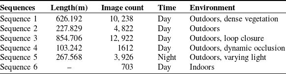
Self-collected datasets: We collected six sequences in different environments for evaluation (Table I). In Sequence 1, the multi-camera rig moves away from buildings and passes through dense vegetation. The sparse, repetitive visual features in this environment challenge visual SLAM. Sequence 2 was collected in an ordinary outdoor environment without deliberately introducing particular difficulties. Since visual SLAM systems accumulate drift over time, loop closure is important for error correction. Sequence 3 was therefore designed to evaluate loop closure: the rig moves around several buildings and returns to a previously observed area. We also collected sequences under more challenging outdoor conditions. Sequence 4 follows a route used by campus buses while buses are passing, producing dynamic-object occlusions. This setting poses significant challenges for purely visual SLAM systems due to the reduction in available static information and the increase in dynamic feature points within the camera FoV. Sequence 5 was acquired at night along a road with alternating illuminated and dark sections to evaluate performance under low light and changing illumination. All outdoor data were collected on campus, where pedestrian and vehicle traffic is generally sparse. Figure 7a shows the environments of the five outdoor sequences. For qualitative indoor evaluation, Sequence 6 was collected in a room. Figure 7b presents representative images from each sequence. Except for Sequence 6, all sequences pose substantial challenges to visual SLAM; even the relatively simple sequence 2 exhibits issues such as motion blur.

Table I.

Details of our collected datasets.

Table I. Long description

A table comparing sequences of collected datasets with details on length, image count, time, and environment. The table has six rows and five columns. Column headers are Sequences, Length(m), Image count, Time, and Environment. Row 1: Sequence 1, Length 626.192, Image count 10,238, Time Day, Environment Outdoors, dense vegetation. Row 2: Sequence 2, Length 227.829, Image count 4,822, Time Day, Environment Outdoors. Row 3: Sequence 3, Length 854.706, Image count 12,922, Time Day, Environment Outdoors, loop closure. Row 4: Sequence 4, Length 103.242, Image count 1612, Time Day, Environment Outdoors, dynamic occlusion. Row 5: Sequence 5, Length 267.568, Image count 3,926, Time Night, Environment Outdoors, varying light. Row 6: Sequence 6, Length 703, Image count 703, Time Day, Environment Indoors.

Figure 7.

The environments of sequences and the images from sequences. (a) The environments of sequence 1,2,3,4, and 5. Sequence 5 was collected at night. Sequence 4 includes dynamic object occlusions, and the direction of sequence 2 is opposite to that of sequence 1. (b) The images from sequences.

Figure 7. Long description

Panel A: A map showing the environments of five sequences. The sequences are marked with different colored dashed lines: yellow for Sequence 1, black for Sequence 2, purple for Sequence 3, red for Sequence 4, and blue for Sequence 5. Panel B: Six images from the sequences. Sequence 1 shows a tree-lined path, Sequence 2 shows a road with a pedestrian crossing, Sequence 3 shows a sidewalk with buildings, Sequence 4 shows a bus at night, Sequence 5 shows a road at night with light trails, and Sequence 6 shows an indoor office space.

EuRoC MAV dataset: To complement the self-collected sequences, we also evaluate DAMC-SLAM on the public EuRoC MAV dataset. It comprises 11 indoor sequences acquired in three environments: a machine hall and two Vicon rooms. The sequences are labeled Easy, Medium, or Difficult and encompass diverse motion patterns, illumination conditions, and scene textures. This benchmark therefore provides an additional evaluation of the generalization of DAMC-SLAM beyond our own data.

5.2. Localization accuracy

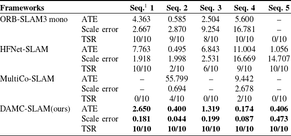
For comparison, we evaluated DAMC-SLAM alongside ORB-SLAM3 [Reference Campos, Elvira, Rodriguez, Montiel and Tardos18], HFNet-SLAM [Reference Liu and Aitken15], and MultiCo-SLAM [Reference Urban and Hinz24]. ORB-SLAM3 was tested in monocular and stereo modes. In monocular mode, the forward-facing Camera 0 was used for Sequences 1, 2, 3, and 5. For Sequence 4, Camera 5 was used because dynamic objects are concentrated in its FoV. In stereo mode, Cameras 0 and 5 were used for all sequences. HFNet-SLAM used the same setup as ORB-SLAM3 in monocular mode. MultiCo-SLAM and DAMC-SLAM used all available cameras with overlapping FoVs. The number of extracted features from each image was set to 1,000 for all systems. We evaluated all multi-frame trajectories rather than only multi-keyframe trajectories. Before evaluation, trajectories were aligned with the ground truth using Sim(3). We then calculated the absolute trajectory error (ATE). The scale is the Sim(3) alignment parameter $s$ , and scale error is defined as $|s-1|$ . The tracking success rate (TSR) is the number of successful trials divided by the total number of trials. All reported results are the averages of 10 runs. A trial is considered successful when fewer than 20 frames have failed tracking.

Table II.

Comparison of localization accuracy (RMS ATE in m), scale error, and tracking success rate on self-collected $^*$ .

Table II. Long description

A table comparing localization accuracy (RMS ATE in meters), scale error (percent), and tracking success rate (TSR) across different frameworks for various sequences. The table has 5 columns and 17 rows, including headers. Column headers are Seq. 1, Seq. 2, Seq. 3, Seq. 4, and Seq. 5. Row labels include ORB-SLAM3 mono, HFNet-SLAM, MultiCo-SLAM, and DAMC-SLAM(ours). Each framework has values for ATE, Scale error, and TSR across the sequences. Notable trends include DAMC-SLAM(ours) showing the lowest ATE and scale error values, and a perfect TSR of 10/10 across all sequences. ORB-SLAM3 mono and HFNet-SLAM show higher ATE and scale error values with varying TSR. MultiCo-SLAM has the highest ATE values and lower TSR.

$^*$ All displayed results are derived from the average of track success trials.

$^1$ “Seq.” stands for “Sequence”.

Table II presents the results for the self-collected dataset. ORB-SLAM3 in stereo mode fails to track all sequences successfully because its two cameras must maintain sufficient overlapping FoVs. Its performance metrics are therefore not reported in table. ORB-SLAM3 in monocular mode tracks most sequences successfully, but its performance degrades substantially under dynamic occlusions and illumination changes. In particular, nighttime illumination changes make initialization difficult. HFNet-SLAM exhibits poorer overall ATE performance and unstable tracking on Sequences 2 and 3. However, its learning-based HFNet feature extractor provides strong robustness on Sequence 5 under varying illumination. MultiCo-SLAM also struggles to track all sequences. Although it achieves partial success on Sequences 2 and 4, its ATE remains unsatisfactory. DAMC-SLAM achieves the lowest average ATE and scale error across the evaluated sequences. It successfully tracks all trajectories, including those affected by dynamic-object occlusions and nighttime illumination changes. These results indicate strong robustness under challenging conditions. This result can be primarily attributed to the integration of multi-camera systems and CNNs. Specifically, CNN-based feature points exhibit higher stability, and the extracted local descriptors demonstrate stronger robustness against disturbances induced by variations in viewing angles, lighting conditions, and other confounding factors. In addition, the multi-camera system provides richer environmental information. When tracking fails, the multi-camera relocalization module enables efficient recovery. Together, these characteristics improve significantly the overall accuracy and robustness of the system. DAMC-SLAM also generates maps with scale closest to the ground truth because it effectively uses stereo information. Figure 8 compares the trajectories of the evaluated systems with the ground truth for Sequences 2, 4, and 5. Neither the monocular nor stereo mode of ORB-SLAM3 completed Sequence 5 successfully; their results are therefore omitted from Figure 8(c).

To complement the self-collected sequences and contextualize the performance of DAMC-SLAM on an established benchmark, we conducted experiments on the EuRoC dataset and compared it with ORB-SLAM3 and HFNet-SLAM. All methods used the left camera of the dataset as input, and each sequence was evaluated 10 times with the mean result reported.

Table III reports the RMSE results on the EuRoC MAV dataset. Although DAMC-SLAM is designed for arbitrary multi-camera configurations rather than specifically for monocular operation and does not employ an image pyramid, it achieves performance comparable to the two monocular baselines. DAMC-SLAM matches or outperforms ORB-SLAM3 on 8 of the 11 sequences, while the monocular baselines perform better on some individual sequences. Notably, DAMC-SLAM obtains the lowest average RMSE of 0.087 m, compared with 0.106 m for HFNet-SLAM and 0.129 m for ORB-SLAM3. These results indicate that the proposed system retains competitive accuracy even when evaluated with a single-camera input, while its multi-camera design does not compromise its overall generalization on EuRoC.

Table III.

Comparison of localization accuracy (RMS ATE in M) on EuRoC.

Long description

The table presents a comparison of localization accuracy, measured in Root Mean Square Error (RMSE) in meters, across different frameworks on the EuRoC dataset. It includes data for three frameworks: ORB-SLAM3, HFNet-SLAM, and a third framework labeled as ‘Ours’. The table has 11 columns representing different sequences (MH01, MH02, MH03, MH04, MH05, V101, V102, V103, V201, V202, V203) and an additional column for the average RMSE. Row 1: ORB-SLAM3, 0.022, 0.024, 0.029, 0.281, 0.158, 0.034, 0.035, 0.194, 0.276, 0.024, 0.337, 0.129. Row 2: HFNet-SLAM, 0.015, 0.021, 0.043, 0.060, 0.825, 0.032, 0.023, 0.023, 0.019, 0.013, 0.097, 0.106. Row 3: Ours, 0.022, 0.023, 0.044, 0.107, 0.062, 0.034, 0.187, 0.030, 0.025, 0.017, 0.401, 0.087.

Figure 8.

Comparison of trajectories with the ground truth for sequences 2,4, and 5. Due to the failure of ORB-SLAM3 to operate successfully on sequence 5, it is not presented in (c).

5.3. Loop closure

Loop closure is essential for mitigating cumulative errors in SLAM. Sequence 3 contains a loop and is used to evaluate this capability; the quantitative results are reported in Table II. MultiCo-SLAM failed in all 10 trials. Although HFNet-SLAM adopts HFNet, a learning-based feature extractor, it succeeded in only 6 of 10 trials. ORB-SLAM3 in monocular mode succeeded in 8 trials, whereas DAMC-SLAM achieved a 100% success rate. Note that, our DAMC-SLAM does not employ an image pyramid for feature extraction. The achievement of comparable performance can be attributed to two key factors: first, the adoption of CNN-extracted global descriptors for loop closure detection, and second, the rich information provided by the multi-camera system. With respect to the ATE metric, our DAMC-SLAM system achieved an error of 1.319 m, representing an approximate 47% improvement compared to ORB-SLAM3 (monocular mode), which exhibited an ATE of 2.504 m. Compared with HFNet-SLAM, which also adopts the learning-based feature extraction method, it achieves an improvement of 81%. Regarding the scale error, our method reduced it to 0.199. ORB-SLAM3 in monocular mode cannot recover metric scale, and its stereo mode failed because the cameras must maintain sufficient overlapping FoVs. Figure 9 shows maps created by DAMC-SLAM, which can be compared qualitatively with the satellite image. The EuRoC experiments also demonstrate loop-closure capability of DAMC-SLAM under a monocular configuration. Figure 10 shows trajectories of selected EuRoC sequences containing loop closures. In summary, our proposed method not only achieves effective loop closure detection but also leverages loop closure effectively and adequately to correct maps and mitigate cumulative errors.

Figure 9.

Map qualitative assessment. The dashed line in (b) represents the ground truth trajectory of sequence 3.

Figure 10.

Loop closure results on the EuRoC dataset.

5.4. Effect of camera configurations

To evaluate the impact of different camera configurations on the DAMC-SLAM system, experiments were conducted under both overlapping and nonoverlapping FoVs scenarios with varying camera numbers. The test sequences selected included sequence 2 (collected from normal environmental conditions) as well as sequence 4 and sequence 5 (collected from extreme conditions). Each experimental group was repeated 10 times to ensure statistical reliability.

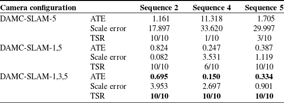
Table IV shows the effect of camera configuration under nonoverlapping FoVs. Because dynamic objects in Sequence 4 appear in the FoV of Camera 5, cameras were added incrementally from Camera 5 to improve comparability. All configurations completed Sequence 2 successfully. In Sequences 4 and 5, however, the single-camera configuration did not provide stable tracking. It succeeded in only 1 of 10 trials on Sequence 4 and 3 of 10 trials on Sequence 5. Notably, when the number of cameras was increased to three, a 100% success rate was attained across all test sequences. The ATE also improved gradually as the number of cameras increased. Scale error remained unstable because nonoverlapping configurations provide no stereo information to recover metric scale. For deployments with purely nonoverlapping FoVs, future work could fuse IMU measurements, wheel odometry, or other metric sensors to provide an additional scale constraint.

Table IV.

Evaluation of different camera configurations with nonoverlapping FoVs.

Table IV. Long description

The table presents the evaluation of different camera configurations with nonoverlapping FoVs across three sequences. It has four rows and three columns. The column headers are Sequence 2, Sequence 4, and Sequence 5. The row labels are Camera configuration, ATE, Scale error, and TSR. Row 1: Camera configuration, DAMC-SLAM-5, DAMC-SLAM-1,5, DAMC-SLAM-1,3,5. Row 2: ATE, 1.161, 0.824, 0.695; 11.318, 0.247, 0.150; 1.705, 0.387, 0.334. Row 3: Scale error, 17.897, 0.082, 3.953; 33.620, 3.531, 2.697; 29.997, 1.119, 0.901. Row 4: TSR, 10/10, 10/10, 10/10; 1/10, 6/10, 10/10; 3/10, 10/10, 10/10.

Table V.

Evaluation of different camera configurations with overlapping FoVs.

Table V. Long description

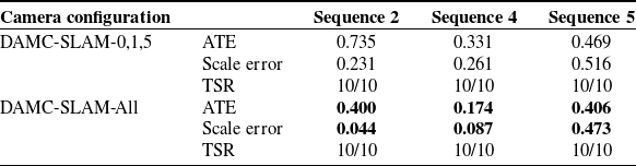
The table presents the evaluation of different camera configurations with overlapping FoVs across three sequences. It has three rows and five columns. The columns are labeled as Camera configuration, Sequence 2, Sequence 4, and Sequence 5. The row labels are DAMC-SLAM-0,1,5 and DAMC-SLAM-All. Each row provides values for ATE, Scale error, and TSR for the respective sequences. Row 1: DAMC-SLAM-0,1,5, Sequence 2 ATE 0.735, Scale error 0.231, TSR 10/10, Sequence 4 ATE 0.331, Scale error 0.261, TSR 10/10, Sequence 5 ATE 0.469, Scale error 0.516, TSR 10/10. Row 2: DAMC-SLAM-All, Sequence 2 ATE 0.400, Scale error 0.044, TSR 10/10, Sequence 4 ATE 0.174, Scale error 0.087, TSR 10/10, Sequence 5 ATE 0.406, Scale error 0.473, TSR 10/10.

We also evaluated DAMC-SLAM under two configurations with overlapping FoVs: Cameras (0, 1, 5) and all cameras. Adjacent cameras were configured with overlapping FoVs to provide stereo information. Table V presents the results. The system achieved a 100% tracking success rate for every configuration and test sequence, demonstrating its robustness. In terms of the ATE metric, the system performance gradually improved with the increase in the number of cameras, and the optimal performance was achieved when all cameras were employed. Owing to the configured overlapping FoVs between cameras, the system was provided with available stereo information. It can be observed from the scale error metric that the scale error decreased progressively as the number of overlapping FoV increased. This phenomenon confirms that the system can effectively utilize stereo information to recover metric scale.

Overall, DAMC-SLAM can operate with arbitrary multi-camera configurations. This capability results from optimizations throughout the system. The hybrid initialization module provides reliable initialization, whereas the tracking, local mapping, and loop closure modules exploit multi-camera information while filtering interference. As a result, the system exhibits a tendency where its performance metrics gradually improve with the increase of input information, rather than diverging due to the introduction of interference.

5.5. Filtering and retention of potential dynamic features

In the motion-model tracking module, map points are projected using the pose predicted by the constant-velocity model for feature matching. When only a few feature points lie on dynamic objects, their interference with pose estimation is limited. The resulting accurate pose estimate further reduces matches to dynamic features in subsequent frames. Figure 11 compares results without and with potential dynamic feature filtering. In the first row, panels (a)–(c) illustrate the increasing influence of dynamic objects as their image coverage increases. Panels (a) and (b) show that the system is inherently robust to small dynamic objects. In contrast, the large dynamic object in panel (c), which occupies more than one-sixth of the image, still affects the system. The second row shows the results after filtering. Panels (d) and (e) show that the threshold-based dynamic-feature filtering strategy remains robust to small dynamic objects, whereas panel (f) demonstrates effective suppression of the interference caused by the large dynamic object.

Figure 11.

Illustration of potential dynamic features filtering. The first row shows feature points before filtering, and the second row shows feature points after filtering. Green features serve as the features for successful tracking.

Figure 12 further illustrates the filtering and retention of potential dynamic features under different dynamic-object distributions. Panels (b)–(e) show that the strategy effectively retains features on stationary objects classified as potentially dynamic across different spatial distributions. It can also retain such features when the segmentation model produces erroneous labels, as demonstrated by the building features in panel (e). However, as shown in panel (f), features are also filtered when the semantic masks associated with stationary objects classified as potentially dynamic occupy a large portion of the image. This limitation warrants further improvement, but it does not affect pose estimation when sufficient other features are available for pose optimization.

Figure 12.

Examples of filtering and retaining potential dynamic features under different dynamic-object distributions. Pink points indicate successfully tracked features on stationary objects classified as potentially dynamic, whereas green points indicate successfully tracked features on static background regions.

5.6. Run time performance

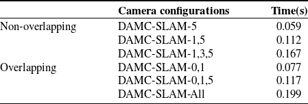
Table VI presents the average processing time per multi-frame for different camera configurations. The experiments used Sequence 2 and included the Camera (0, 1) configuration to measure runtime with the minimum stereo information. Under nonoverlapping FoVs, DAMC-SLAM achieves a maximum speed of 17 fps, which decreases to 6 fps with three cameras. Under overlapping FoVs, the maximum speed is 13 fps and decreases to 5 fps when all six cameras are used. Considering that the system needs to handle a $360^{\circ } \times 180^{\circ }$ stereo FoV, this processing speed is acceptable. The main bottlenecks are CNN-based preprocessing and local-map tracking. Under the DAMC-SLAM-All configuration, frame processing and local-map tracking require approximately 85 and 92 ms, respectively, accounting for approximately 89% of the total processing time reported in Table VI. Within local-map tracking, local-point matching requires approximately 67 ms and is the dominant cost, whereas pose-only bundle adjustment requires approximately 17 ms. Future improvements could be achieved by deploying a lighter or quantized CNN and by reducing the local-point search workload through adaptive selection of keyframes and map points.

Table VI.

The average time consumed per multiframe at different camera configurations.

Table VI. Long description

A table with two rows and three columns comparing the average time consumed per multiframe at different camera configurations. The table is divided into two groups: Non-overlapping and Overlapping. Under Non-overlapping, the camera configurations and their respective times are: DAMC-SLAM-5 with 0.059 seconds, DAMC-SLAM-1,5 with 0.112 seconds, and DAMC-SLAM-1,3,5 with 0.167 seconds. Under Overlapping, the camera configurations and their respective times are: DAMC-SLAM-0,1 with 0.077 seconds, DAMC-SLAM-0,1,5 with 0.117 seconds, and an unnamed configuration with 0.199 seconds.

5.7. Indoor performance

DAMC-SLAM also operates indoors. Sequence 6 was collected in a room using the multi-camera rig. Figure 13(b) shows one multi-frame, and Figure 13(a) shows the resulting map. The map appears cluttered because the system extracts features from the ceiling and floor. We therefore show a map produced shortly after initialization for clarity. Prominent objects from which map points are extracted are labeled in Figure 13(a), and their locations are shown in Figure 13(b). The result demonstrates that DAMC-SLAM captures indoor spatial features and generates an accurate trajectory and map.

Figure 13.

Indoor performance on sequence 6.

Figure 13. Long description

Panel A: A map created indoors by DAMC-SLAM. The map shows a 3D point cloud with red dots representing the environment and green lines indicating the camera trajectory. Inset images show specific frames with green bounding boxes highlighting detected features. Panel B: A multi-frame visualization from DAMC-SLAM. The image shows a sequence of indoor scenes with green dots and lines overlaying the images, representing detected features and camera movements.