


1 Introduction
Consignment sampling is a key component of quality assurance, underpinning the trade in horticultural produce. Methodologies for the sampling of consignment lots are described in International Standards for Phytosanitary Measures (ISPM) No. 31, Methodologies for sampling of consignments [3]. A key objective of sampling of consignments is to “provide assurance that the number of regulated pests or infested units in a consignment does not exceed the specified tolerance level for the pest” [3], a form of compliance sampling [Reference Schilling and Neubauer6]. Typically, a
$600$
 -piece sample is taken from a consignment for inspection, which, if no infested items are found, provides 95% confidence that the underlying prevalence of infested is no more than 0.5% (1 in 200). These calculations assume that the inspection sensitivity to detect infection is 100%, and that either the sample is random or the consignment is well mixed. The acceptance level (that is, the number of infested units detected before the consignment is rejected) is typically set to zero. The ISPM further detail methods of calculating the power of consignment sampling to detect a specified underlying (“design”) prevalence [3].
For internal pests such as fruit flies from the Tephritidae family [Reference White7], infestation generates few if any visible symptoms and nondestructive visual inspection of consignment samples has a very low sensitivity to detect infested fruit. In contrast, destructive sampling methods, such as the slicing of fruit [Reference Gould4] or applying brown sugar flotation to crushed samples of fruit [Reference Balagawi, Broughton, Liang, Archer, Cruickshank, Cruickshank, Barchia and Stevens1, Reference Yee9], provide much higher detection sensitivity for such pest species. Such methods are rarely employed due to the loss of product involved (typically a minimum of
$600$
 pieces per consignment). We note, however, that fruit rejected as part of the sorting and grading procedure within the pack house [Reference Masuda, Uchida, Fujita, Miyamoto, Yasue, Kubo, Ushijima, Uchida and Akagi5] may be subject to destructive inspection without production loss. Furthermore, larger samples of fruit can potentially be inspected than the typical
$600$
 -piece consignment sample.
In this paper, we explore quantitatively how sampling from the reject bin can be used to provide additional inference on the phytosanitary state of a horticultural consignment subject within a compliance sampling framework. Of particular interest is how selective the grading and ultimately rejection process is with respect to the infection status of the fruit, and how this impacts on the estimated prevalence of infestation within consignments, given the sampling data.
2 Materials and methods
2.1 Production system description
Following harvest from the orchard, picked fruit are brought into the pack house for grading and sorting (Figure 1(a)), the basis of which can include selection related to marketability, eating quality and/or the presence of physical symptoms indicative of disease. The process is becoming increasingly mechanized, using optical grading machines that are capable of classifying individual fruit on the basis of size, weight, shape and colour features. During the grading and sorting process, fruit may end up being rejected for reasons including being too big, too small, not sufficiently ripe (“green”), overly ripe (“soft”), having unwanted colour, being misshapen, blemished or visibly damaged. These fruit end up in the “reject” bin (Figure 1(b)). The proportion of fruit that is “rejected” may be influenced by the crop type, growing conditions, pest prevalence and target market, and is typically a nontrivial proportion of the harvest.
Schematic of the production process, including (a) fruit production and harvest, (b) grading, sorting and packing/rejection, (c) inspection of consignment of reject bin samples, (d) inference on infestation level within packed fruit, and (e) packed fruit bound for market with associated inferred infestation status. (The schematic illustration was provided by Brent Henderson.)

Figure 1 Long description
A schematic showing an orchard, then a packing house, then grading. Accepted fruit go into consignment, then standard 600 fruit consignment sampling. Rejected fruit go to the reject bin, then reject bin sampling. Both samples are used for combined inference across consignment and reject bin about infestation level. The consignment then goes to market.
We consider two inspection compliance measures, namely consignment sampling and reject bin sampling (Figure 1(c)). Consignment sampling involves the inspection of samples drawn from the consignment of packed product. Generally the inspection associated with consignment samples is restricted to being nondestructive (visual only), and hence the inspection sensitivity is typically low for internal pests (for example, fruit fly larvae). Reject bin sampling involves the inspection of samples drawn from fruit that have been “rejected” for packing and placed in the reject bin. Destructive inspection of these sample incurs no production losses, and can include slicing and brown sugar flotation, resulting in considerably higher detection sensitivities in comparison to visual inspection.
The data arising from the samples are used to make inference (Figure 1(d)) on the infestation level of fruit that is potentially bound for market (Figure 1(e)).
2.2 Model description
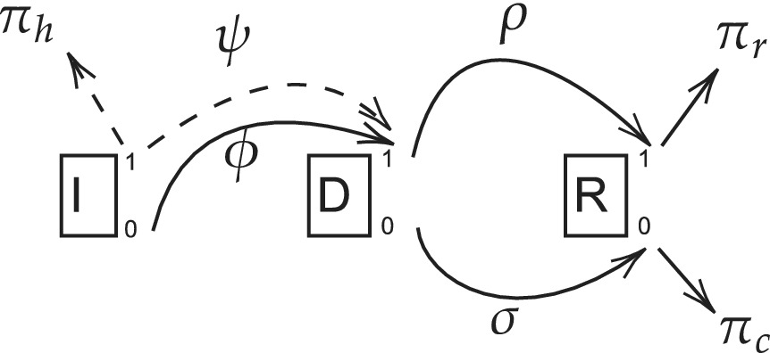
To undertake detection probability calculations on the basis of inspection samples, we need to estimate the prevalence of infested fruit within both the reject bin and the associated consignment of packed product: this will be affected by the visual properties of infested and uninfested fruit in combination with the selectivity of grading with respect to fruit infestation status. We then estimate the sensitivity and specificity of the inspection procedures as applied to samples from the consignment and the reject bin. To do this, we define the following binary random variables (see Figure 2):
-
• $I=1$
 when a piece of fruit is infested/infected by a pest/pathogen, and
$I=0$
otherwise;
-
• $D=1$
when a piece of fruit has defective features (too big, too small, blemished, wrong colour, …), noting that defective features are considered as being potentially detectable during the grading process, and
$D=0$
otherwise; and -
• $R=1$
when a piece of fruit is rejected for packing during grading and placed in the reject bin, and
$R=0$
otherwise.


Model description, with I = infested, D = defective and R = rejected. Solid arrows between binary states represent parameters defined by the conditional probability of the state at the arrow head, given the state at the arrow tail. For example,
$\phi = P(D=1|I=0)$
 . Solid arrows pointing away from a state represent probabilities of infection (
$I=1$
 ) given the state at the arrow tail. Dashed arrows represent exceptions:
$\pi _h$
 is simply the unconditional probability
$P(I=1)$
 and
$\psi $
 is related to
$P(D=1\mid I=1)$
 via equation (2.1).

Figure 2 Long description
A diagram representing events I=Infested, D=Defective and R=Rejected as boxes, each with a 0 and a 1 representing the binary states each can have. There are solid arrows between some of these, representing a conditional probability, labelled with the relevant parameter. These are: phi as the probability of D=1 given I=0, rho as that of R=1 given D=1, and sigma as that of R=0 given D=0. There are two solid arrows pointing away from a state; these are pi_r as the probability of infection (I=1) given R=1, and pi_c as that of I=1 given R=0. Two dashed arrows represent exceptions, where pi_h is the unconditional probability of infection, and psi is given by equation 1.
Next, we define the conditional probabilities relating to screening sensitivity and specificity:
-
• $\phi =P(D=1\mid I = 0)=P(\text {Defective}\mid \text {Not infested})=$
base rate of defective fruit in absence of infestation; -
• $\rho =P(R=1\mid D=1)=P(\text {Rejected}\mid \text {Defective})=$
grading sensitivity; and -
• $\sigma =P(R = 0\mid D = 0)=P(\text {Not rejected} \mid \text {Not defective})=$
grading specificity.


Let
$\psi =P(I \rightarrow D)=P(\text {Infestation generates physical defects})$
 —that is, the propensity of infestation to generate physical symptoms that could be considered defective. For example, in the case of codling moth, infestation can cause defects in the form of tunnelling holes. It is defined such that

where we assume independence between the innate propensity of fruit to exhibit defects (that is,
$\phi $
 ) and the state of being infested. When
$\psi = 0$
 , infestation and defects are independent, that is,
$P(D=1\mid I=1) = \phi = P(D=1\mid I=0)$
 . When
$\psi = 1$
 , the presence of infestation guarantees defects, that is,
$P(D=1\mid I=1) = 1$
 . Then the probability of harvested fruit being defective is

where
$\pi _h= P(I=1)$
 , the prevalence of infestation in harvested fruit entering the pack house (prior to grading).
Further, define the underlying prevalence of infestation following grading as follows:
$\pi _r$
 is the prevalence of infestation among rejected fruit; and
$\pi _c$
 is the prevalence of infestation among the nonrejected (that is, packed) consignment of fruit.
The prevalence of infestation in the packed consignment is the measure of primary interest from a risk perspective, and is the prevalence within fruit conditional on it not being rejected during grading. That is,
$\pi _c = P(I=1\mid R = 0)$
 . The prevalence of fruit in the reject bin is
$\pi _r = P(I=1\mid R=1)$
 . These probabilities are computed using Bayes’ theorem, but first some conditional probabilities of rejection given infestation state are needed. We have

Likewise,

For the prevalence within the packed consignment (that is, the event “Not rejected”), applying Bayes’ theorem gives

Likewise, the prevalence within the reject bin (that is, the event “Rejected”) is calculated as

where

and

2.3 Extending the ISPM31 approach
The ISPM31 sampling protocol and associated calculations focus on the risk (“confidence level”) of a user-specified design prevalence (“level of detection”) being exceeded, given no detections from within a consignment sample of known size and detection efficacy. This frequentist approach for undertaking compliance sampling can be extended to having no detections in either a consignment sample or a sample from the associated reject bin. To facilitate this, let:
-
• $n_{rs}$
be the number of fruit sampled from the reject bin; and -
• $n_{cs}$
be the number of fruit sampled from the consignment.


For the sensitivity of inspection for the different measures, we have:
-
• $\delta _{cs}$
is the detection sensitivity applied to samples from the packed consignment, combining both the probability of an infested piece exhibiting symptoms of infestation being detected (here we are assuming by the human eye) and the subsequent diagnostic method confirming infestation; and -
• $\delta _{rs}$
is the sensitivity of diagnostic method applied to samples from the reject bin sample, applied regardless of physical symptoms.


The values of both
$\delta _{cs}$
 and
$\delta _{rs}$
 depend on the method of inspection and associated diagnostic procedure. We assume here that the inspection of the consignment sample is a two-step process starting with visual screening, followed by a diagnostic examination (for example, slicing) for pieces detected as showing symptoms (defects). Hence, to apply
$\delta _{cs}$
 within calculations we need to estimate the proportion of infested fruit within the consignment (not rejected during grading) that exhibit defects. That is,

where

hence

With respect to the sampling data let:
-
• X be the number of detections from consignment sampling; and
-
• Y be the number of detections from reject bin sample.
Assuming that the numbers of fruit within the consignment and reject bin are large in comparison to the respective samples
$n_{cs}$
 and
$n_{rs}$
 , the Poisson approximation to the binomial is appropriate [Reference Yamamura, Katsumata, Yoshioka, Yuda and Kasugai8], and the probability of detecting at least one infested fruit given the underlying prevalence, inspection and grading parameters (designated
$\boldsymbol {\theta }$
 ) is

where
$\pi _c$
 and
$\pi _r$
 are calculated as in equations (2.2) and (2.3). Note that we have not included the proportion of infested fruit within the reject bin that exhibit symptoms in equation (2.4), as it is assumed that the fruit sampled for inspection are chosen without regard to defect status, and are all subjected to the same diagnostic investigation (for example, slicing). Note also that X and Y are conditionally independent given prevalence. We derive the prevalence of defects amongst infested fruit consigned to the reject bin in Appendix A should readers want to modify equation (2.4) to account for only inspecting symptomatic fruit from the reject bin.
Calculating
$\pi _c$
 such that the power to detect at least one infested fruit is at a desired confidence level (for example, 95%) is undertaken numerically. That is, for a given value of
$\pi _h$
 , we calculate the corresponding values of
$\pi _c$
 and
$\pi _r$
 , and from these the probability of at least one detection occurring (using equation (2.4)), from the consignment sample (
$X>0)$
 and/or the reject bin sample (
$Y>0$
 ).
2.4 Measuring effectiveness of reject bin sampling
The conditional probability
$P(X=0 \mid Y>0)$
 gives us the probability that consignment sampling would have missed an infestation given that the reject bin sampling found an infestation. This gives us a measure of effectiveness of sampling: if the probability is low, then reject bin sampling is not worth pursuing as it is unlikely to add anything; conversely, if the probability is high, then it is.
2.5 Use cases of interest
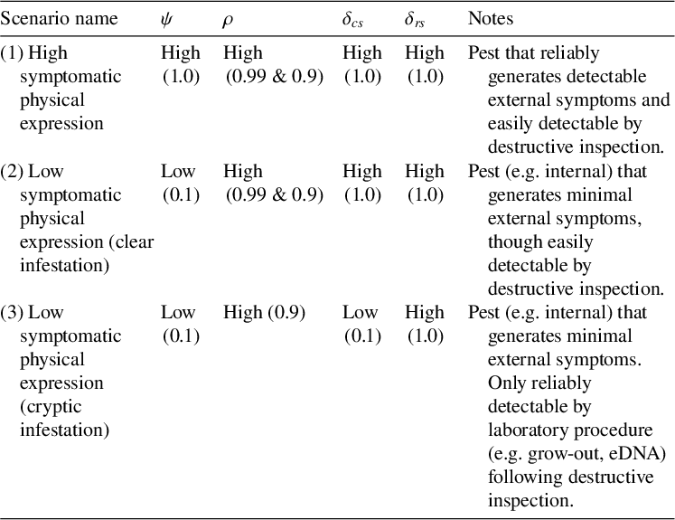
We focus on three general scenarios to evaluate how inspecting rejected samples will affect the phytosanitary state of the packed consignment. First, in Scenario 1, we examine high symptomatic physical expression that is readily detectable by both human observation and machine grading, with visual confirmation following destructive sampling. For the other scenarios, we examine low symptomatic physical expression of infestation, where symptomatic units are still detectable by both human observation and machine grading: for Scenario 2, visual confirmation is straightforward following destructive sampling; but for Scenario 3 it is of low sensitivity as laboratory procedures are required. Details are provided in Table 1. We restrict our inference to single consignment samples of size 600, though note that combining the results from multiple consignment samples can provide stronger evidence for low levels or absent infestation [Reference Caley, Gladish, Kingham and Van Klinken2].
Details of use case scenarios for the inspection of samples from the reject bin in terms of
$\psi $
 (the probability of an infested piece of fruit exhibiting a defect),
$\rho $
 (the probability of a piece of fruit with a defect being rejected during grading) and the inspection sensitivity for samples from consignments (
$\delta _{cs}$
 ) and the reject bin (
$\delta _{rs}$
 ).

Table 1 Long Description
Details of use case scenarios for the inspection of samples from the reject bin in terms of psi (the probability of an infested piece of fruit exhibiting a defect), rho (the probability of a piece of fruit with a defect being rejected during grading) and the inspection sensitivity for samples from consignments (delta_cs) and the reject bin (delta_rs). Scenario 1 is named High symptomatic physical expression with psi=1.0, rho=0.99 & 0.9, delta_cs=1.0 and delta_rs=1.0. This represents a pest that reliably generates detectable external symptoms and easily detectable by destructive inspection. Scenario 2 is named Low symptomatic physical expression (clear infestation) with psi=0.1, rho=0.99 & 0.9, delta_cs=1.0 and delta_rs=1.0. This represents a pest (e.g. internal) that generates minimal external symptoms, though easily detectable by destructive inspection. Scenario 3 is named Low symptomatic physical expression (cryptic infestation) with psi=0.1, rho=0.9, delta_cs=0.1 and delta_rs=1.0. This represents a pest (e.g. internal) that generates minimal external symptoms, and is only reliably detectable by laboratory procedure (e.g. grow-out, eDNA) following destructive inspection.
3 Results and discussion
3.1 High symptomatic physical expression scenario
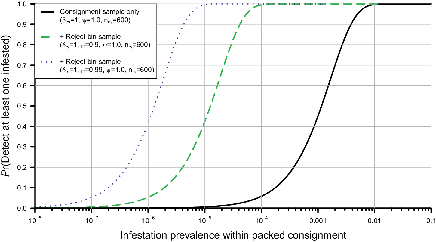
Under this near-optimal scenario, the expression of physical defects given infestation is perfect (
$\psi =1$
 ), the prevalence of defects arising from benign sources is low (
$\phi =0.1$
 ), the grading sensitivity is high (
$\rho =0.9$
 and
$\rho =0.99$
 illustrated) and highly specific (
$\sigma =1$
 ), and the inspection sensitivities perfect (
$\delta _{cs}=\delta _{rs}=1$
 ). Here, the additional inspection of a
$600$
 -piece sample from the reject bin reduces the upper bound of infection by about two orders of magnitude when
$\rho = 0.9$
 , and three orders of magnitude when
$\rho = 0.99$
 (Figure 3).
The effect of adding a
$600$
 -piece sample inspection from the reject bin in addition to a single
$600$
 -piece sample inspection from the consignment (solid line), for a scenario where the pest reliably generates defective features that can be screened for with either high (
$\rho =0.9$
 ) or very high (
$\rho =0.99$
 ) sensitivity. Parameter settings are for Scenario 1: “High symptomatic physical expression” (see the text for full details).

Figure 3 Long description
The effect of adding a 600 piece sample inspection from the reject bin in addition to a single 600 piece sample inspection from the consignment, for a scenario where the pest reliably generates defective features that can be screened for with either high (rho=0.9) or very high (rho=0.99) sensitivity. Parameter settings are for Scenario 1: High symptomatic physical expression. For consignment only, the probability of detecting at least one infested fruit increased from near zero at consignment prevalence around 0.01% to near one at 10%. For rho=0.9, the probability went from near zero around 0.0001% to near one at 0.01%. For rho=0.99, it went from near zero around 0.00001% to near one at 0.001%.
3.2 Low symptomatic physical expression scenario
This scenario differs from the previous one in that the probability that an infested piece of fruit exhibits symptomatic defects is low (
$\psi =0.1$
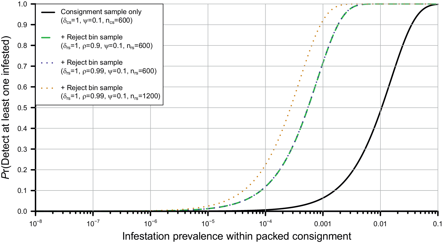
 ). This generates very different results in terms of the power to detect specified prevalence in post-harvest fruit. From a clear inspection of a
$600$
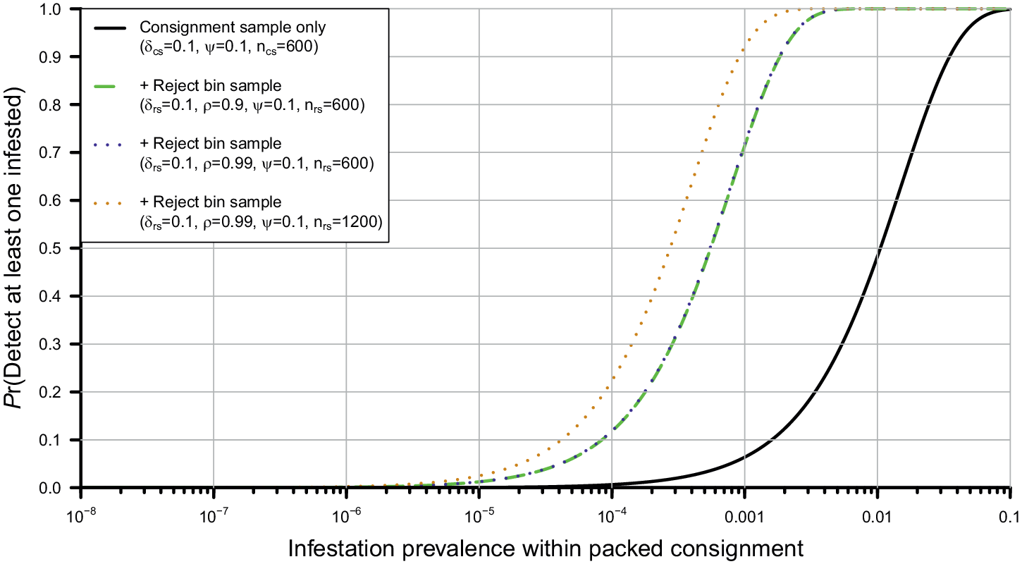
 -piece sample from the packed consignment alone, a much higher prevalence of infestation can go undetected within the consignment (Figure 4). The addition of the inspection of a
$600$
 -piece sample obtained from fruit arising from grading with
$\rho =0.9$
 shifts the cumulative distribution of the possible underlying prevalence by more than an order of magnitude lower. However, increasing the sensitivity of the grading process to near perfect (
$\rho =0.99$
 ), produces virtually no detectable improvement on this (Figure 4). This somewhat surprising result arises from the increase in
$\rho $
 , because (1) the prevalence of infestation within the rejected component does not change, as noninfested though defective fruit are also rejected with the same higher probability, and (2) the extra detection sensitivity is only operating on a small (
$\psi = 10\%$
 ) proportion of infested fruit that are exhibiting physical defects. Increasing the number of fruit inspected from the rejected component does shift the cumulative distribution of the underlying prevalence to the left. For example, doubling
$n_{rs}$
 to 1200 produces a modest additional reduction (Figure 4).
The effect of adding either a
$600$
 - or
$1200$
 -piece sample inspection from the reject bin in addition to a single
$600$
 -piece sample inspection from the consignment (solid line), for a scenario where the pest does not reliably generate defective features that can be screened for with either high (
$\rho =0.9$
 ) or very high (
$\rho =0.99$
 ) sensitivity. Parameter settings are for Scenario 2: “Low symptomatic physical expression (clear infestation)” (see the text for full details).

Figure 4 Long description
The effect of adding either a 600 or 1200 piece sample inspection from the reject bin in addition to a single 600 piece sample inspection from the consignment (solid line), for a scenario where the pest does not reliably generate defective features that can be screened for with either high (rho=0.9) or very high (rho=0.99) sensitivity. Parameter settings are for Scenario 2: Low symptomatic physical expression (clear infestation). For consignment only, the probability of detecting at least one infested fruit increased from near zero at consignment prevalence around 0.1% to near one at 10%. For rho=0.9 or 0.99 and 600 fruit, the probability went from near zero around 0.001% to near one at 0.2%. For rho=0.99 and 1200 fruit, it went from near zero around 0.001% to near one at 0.1%.
3.3 Low symptomatic physical expression with cryptic infestation scenario
Under a scenario where it is very difficult to detect pests even by destructive inspection (
$\delta _{cs}=0.1$
 ), the power to infer a low design prevalence is greatly reduced (Figure 5). The ability to make inference by inspecting samples obtained from the reject bin remains little changed from the scenario where infestation is not cryptic.
The effect of adding either a
$600$
 - or
$1200$
 -piece sample inspection from the reject bin in addition to a single
$600$
 -piece sample inspection from the consignment (solid line), for a scenario where the pest does not reliably generate defective features that can be screened for with either high (
$\rho =0.9$
 ) or very high (
$\rho =0.99$
 ) sensitivity. Parameter settings are for Scenario 3: “Low symptomatic physical expression (cryptic infestation)” (see the text for full details).

Figure 5 Long description
The effect of adding either a 600 or 1200 piece sample inspection from the reject bin in addition to a single 600 piece sample inspection from the consignment (solid line), for a scenario where the pest does not reliably generate defective features that can be screened for with either high (rho=0.9) or very high (rho=0.99) sensitivity. Parameter settings are for Scenario 3: Low symptomatic physical expression (cryptic infestation). For consignment only, the probability of detecting at least one infested fruit increased from near zero at consignment prevalence around 0.1% to near one at 10%. For rho=0.9 or 0.99 and 600 fruit, the probability went from near zero around 0.001% to near one at 0.2%. For rho=0.99 and 1200 fruit, it went from near zero around 0.001% to near one at 0.1%.
3.4 Parameter interactions
The extent to which infested fruit exhibit potentially detectable symptoms is clearly a key quantity, and how this influences the probability of missing any infestation in a consignment depends on the interplay between
$\psi $
 and
$\delta _{rs}$
 . For a given underlying prevalence post-harvest, when
$\psi $
 is high, a high confidence of not missing infestation is achievable with only a low
$\delta _{rs}$
 (Figure 6). If
$\psi $
 is low, however, it becomes impossible to achieve high confidence regardless of the sensitivity of inspection of samples from the reject bin (Figure 6). The possibility of detecting extremely low prevalence (for example, one in 1 million), and thus potentially discarding high-quality produce is very low: the probability only increases beyond 5% when both
$\psi $
 and
$\delta _{rs}$
 are extremely close to 1 (Figure 6).
The probability of missed detection based on two parameters
$\psi $
 and
$\delta _{rs}$
 . Other parameters are set to
$\pi _c = 0.005$
 ,
$\delta _{cs}$
 = 0.1,
$n_{cs} = n_{rs} = 600$
 ,
$\rho = 0.9$
 ,
$\sigma = 1$
 ,
$\phi = 0.1$
 . The solid black line represents a probability of 5% of missing detection (that is, 95% probability of detection) where the consignment infestation rate is 0.5%. The dashed line represents a probability of 5% of detecting where the consignment infestation rate is
$\pi _c = 1 \times 10^{-6}$
 (that is, one in 1 million). Probabilities below
$10^{-5}$
 are set to the same yellow colour.

Figure 6 Long description
The x axis represents psi (defective proportion of infected fruit) ranging from 0.0 to 1.0. The y axis represents delta sub r s (reject bin sensitivity) ranging from 0.0 to 1.0. A color scale on the right indicates the probability of missed detection, using a viridis gradient where dark purple represents a high probability of 1 and bright yellow represents a low probability of 10 super minus 5. The data shows a non-linear relationship where the probability of missed detection decreases as both psi and delta sub r s increase. A solid black curve originates near y equals 0.9 on the left and curves downward toward x equals 1.0 on the bottom, demarcating a threshold in the probability space. The region below and to the left of this curve is dominated by dark purple and teal (higher probability of missed detection), while the region above and to the right is dominated by yellow (lower probability of missed detection).
3.5 Challenges in implementation
For pests that reliably generate defective features that can be screened for during grading and sorting, as the screening process becomes increasingly sensitive, such infested fruit are increasingly eliminated from the consignment. They will, however, potentially be detected in reject bin sampling with increasing probability. In fact, for a given pest prevalence at harvest, the likelihood of detecting a pest from within the reject bin sample will increase at the same time as the prevalence within the consignment is reducing. Currently it is typical for the “acceptance number” (that is, the number of infested units or the number of individual pests that are permissible in a sample of a given size before phytosanitary action is taken) to be set at zero by many national plant pest organizations when dealing with quarantine pests [3]. That is, if any pests are detected within a consignment sample, the consignment is rejected. How the detection of pests within the reject bin arising from a highly sensitive screening procedure will be handled is unclear. If the acceptance number for the inspection of samples from the reject bin is also set to zero, we have shown here that where nothing is found, there may be increased confidence that a design prevalence has not been exceeded. However, in situations where grading is highly selective for infested fruit, there may well be a disincentive for producers to implement sampling from the reject bin.
We have assumed independence between defects arising from benign processes, and those arising from infestation. This may not always be the case. For example, green (unripe) fruit that is considered defective (and rejected) based on colour and/or size and may be less preferred for oviposition by insect pests. Under this scenario it is possible for the reject bin to be dominated by unripe and hence uninfested fruit, and inspecting these fruit may provide false confidence in the phytosanitary state of the nonrejected packed fruit unless such grading selectivity details are known and quantified. Changes to the model equations would be needed to account for this. Conversely, situations where inspecting samples from the reject bin will considerably improve the strength of inference include situations where fruit that are more prone to infestation (for example, damaged and/or overripe) are selectively graded for rejection. These are reasons why the inspection of reject bin samples alone is unlikely to be supported. The additional confidence that the inclusion of inspection of samples from the reject bin provides is heavily dependent on the conditional probabilities P(Defective
$|$
 Infested),
$\phi = P$
 (Defective
$|$
 Uninfested) and/or
$\rho = P$
 (Rejected
$|$
 Defective); knowing or being able to make reasonable assumptions for these are key to the method.
3.6 Improvements to inference
The approach we have implemented is consistent with the methodologies for making inference from consignment samples where no pests are found [3]. Assessing the risk from within the consignment where infested fruit are detected in a sample from the reject bin naturally leads to a Bayesian approach to estimation, by which the estimated prevalence within the harvested fruit, the reject bin and the consignment can all be updated on the basis of the sampling data. The Bayesian approach has the added advantage of being able to quantify product integrity in terms of estimated prevalence in the presence of positive detections. Positive detections are potentially problematical, and any detection within the consignment sample is generally considered unacceptable. Detections within the reject bin, however, are more sensibly viewed within the context of the screening sensitivity provided by grading and sorting. For example, highly selective screening will increase the likelihood of infested fruit being detected within samples from the reject bin, though at the same time reduce the prevalence within the consignment sample. Taken to the limit, the screening process becomes a highly effective phytosanitary measure in its own right, and detections from within the reject bin would be less problematical. That said, the absence of detections within a sample from rejected fruit that arises from a grading process that is highly selective for infested fruit will provide the strongest inference for the absence of infestation or an acceptably low prevalence of infestation within a consignment.
4 Conclusions
We have shown that inspection of samples from the reject bin can result in a considerable improvement in the confidence in a consignment’s phytosanitary state, beyond that provided by the inspection of samples from the packed consignment alone. Unsurprisingly, the biggest gains in confidence in product integrity arise when pest infestation produces features that are (1) detectable (that is, able to be classified as defective) during screening with high sensitivity, and (2) discoverable during inspection of samples from the reject bin (with the advantage of destructive sampling being possible). The probability that infested fruit exhibit features that are detectable during grading and sorting is the key driver of the extent to which grading and sampling from the reject bin can improve confidence in product integrity. That said, where the target pest is internal, the ability to apply destructive inspection methods with higher sensitivity to rejected fruit can provide a major relative improvement in comparison with consignment sampling alone using nondestructive inspection with low detection sensitivity. The improvements that can be made are mediated somewhat by a rising base prevalence of defective fruit arising from benign causes, as this limits the extent to which the prevalence of infestation may be concentrated within the reject bin.
A Deriving proportion of infested fruit in reject bin that is symptomatic
It may be necessary to calculate the probability of infested units of fruit in the reject bin exhibiting defective symptoms. This could be the case if only defective units within the reject bin are to be inspected. The following calculations apply:

where

hence

That is, if either grading with respect to infestation status is 100% specific or the probability that an infested piece of fruit exhibits physical symptoms, the proportion of infested fruit within the reject class that exhibit physical symptoms will be 100%, regardless of
$\rho $
 .
Acknowledgements
The authors would like to thank Lloyd Kingham for suggestions to explore sampling from the reject bin in more detail, and Brent Henderson for drawing Figure 1. Rieks van Kinken’s comments on a draft manuscript are also very much appreciated. The project Developing a national systems approach for meeting biosecurity requirements to access key Asian markets was funded by the Hort Frontiers Asian Markets Fund, and is part of the Hort Frontiers strategic partnership initiative developed by Hort Innovation, with co-investment from CSIRO, the Western Australian Department of Primary Industries Resources and Development, the New South Wales Department of Primary Industries, Agriculture Victoria, and contributions from the Australian Government.











 Open access

