1. Introduction
In many countries, motor vehicle fuels are among the most heavily taxed products.Footnote 1 At the same time, motor vehicle use is associated with an unusually diverse variety of externalities, including local and global pollution, traffic congestion, traffic accidents and road damage. Growing alarm about global climate change, relentlessly increasing urban gridlock and world oil market volatility, along with calls from the G20 to phase out fossil fuel subsidies, have all heightened interest in the appropriate level of fuel taxation.
Over the last two decades, there has been a major effort to measure the external costs of motor vehicles in the United States and certain European countries (e.g., De Borger and Proost, Reference De Borger and Proost2001; Quinet, Reference Quinet2004; Parry et al., Reference Parry, Walls and Harrington2007). However, there has not been much of an attempt to estimate external costs for other (in particular, middle- and low-income) countries, so policy makers in many countries may have little guidance on whether their fuels are currently over- or underpriced from an externality perspective. Fuel tax assessments for one country cannot simply be inferred from optimal tax estimates for, say, the United States, as they depend on many local factors (e.g., travel delays, the incidence and composition of highway fatalities and local valuations of health and travel time).
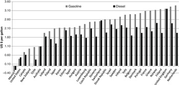
This paper describes an approach to compiling rough estimates of automobile and (commercial) truck externalities, based on combining local data with extrapolations from US literature. The parameters are easily applied to formulas for (second-best) corrective gasoline and diesel fuel taxes.Footnote 2 The analysis is applied to Chile, which is an interesting case study. Its gasoline tax is high relative to rates prevailing in North and South America, but low by OECD standards (see figure 1). Its lighter taxation of diesel fuel relative to gasoline is especially striking, even more so because the modest statutory tax shown in figure 1 is mostly refunded to trucking companies by the government. (Short-run adjustments in tax rates are made to counteract volatility in oil prices, although these price stabilization mechanisms are beyond our scope.)
Excise taxes on gasoline and diesel in OECD countries in year 2010

Reasonable economists could debate endlessly the details of our approach, not least because, due to data limitations, some assumptions must be based on judgment. Nonetheless, establishing a ballpark estimate of the corrective fuel tax based on plausible first-pass assumptions – one that can be refined over time with improved data – is far better than no figure at all. Furthermore, we demonstrate that for most parameters alternative assumptions have relatively modest impacts on corrective taxes.
In our benchmark case the corrective gasoline tax for Chile is US$ 2.35 per gallon, in year 2006 $, or about 60 per cent greater than the prevailing fuel tax. This estimate is substantially larger than comparable calculations for the United States (e.g., Parry and Small, Reference Parry and Small2005) even though the valuation of travel time and health risk is lower in Chile. Offsetting these factors is the much higher accident externality, due to the high incidence of pedestrian fatalities, which is a common feature of lower-income countries (Kopits and Cropper, Reference Kopits and Cropper2008). Moreover, the large share of the country's population residing in Santiago implies that a larger share of nationwide mileage occurs under congested conditions, and a larger share of the population is exposed to elevated pollution–health risks. Higher average fuel economy of the car fleet in Chile (compared to the United States) also magnifies congestion and accident benefits per gallon reduction in gasoline.
As for diesel fuel, our benchmark estimate of the corrective tax is US$ 2.09/gallon (in 2006$). On a per vehicle-mile basis, external costs of trucks are much larger than for cars – for example, trucks take up more road space and contribute more to congestion and, unlike cars, they impose significant road damage externalities. However, an offsetting factor is that the reduction in truck miles per tax-induced reduction in diesel fuel is much smaller than the corresponding reduction in car miles per tax-induced reduction in gasoline.
The most important source of uncertainty in these corrective tax estimates is the valuation of fatality risks from pollution and accidents – for example, with a low valuation of these risks the corrective gasoline tax falls to US$ 1.53 per gallon. All other assumptions relating to vehicle emission rates, initial fuel economy, behavioral responses, marginal travel delays, etc. have far less significance for corrective tax rates. Thus, our basic qualitative finding – that fuels are, if anything, under-taxed, especially in the case of diesel – appears to be robust.
Two further caveats to the analysis are that we do not explore the possibility of externality mitigation through other instruments (e.g., peak-period congestion pricing), or linkages between fuel taxes and the broader fiscal system. These and other limitations are discussed at the end of the paper.
The rest of the paper is organized as follows. The next section provides a brief conceptual framework for corrective fuel taxes. Section 3 discusses the methodology for parameter estimation. Section 4 presents the corrective tax results and sensitivity analysis. Section 5 offers concluding remarks. Appendices for the paper are available online (http://journals.cambridge.org/EDE) and in Parry and Strand (Reference Parry and Strand2011).
2. Externality-correcting fuel taxes: conceptual issues
Fuel taxes are viewed from the perspective of optimizing benefits from vehicle use, net of external costs. We approximate by assuming that gasoline is used by passenger vehicles and diesel by commercial trucks. Therefore (with one caveat noted below), corrective gasoline taxes depend on auto externalities, while diesel taxes depend on truck externalities.Footnote 3
2.1 Corrective gasoline tax
Parry and Small (Reference Parry and Small2005) derive a formula for the (long-run) optimal gasoline tax using a static, homogeneous agent model, where the agent represents an aggregation over all households in the economy. We discuss, very briefly, an adapted version of their model, the most important difference being that we strip out linkages between gasoline taxes and the broader fiscal system (we do this because we lack reliable data for Chile on labor supply responses needed to assess fiscal linkages).
The model boils down to the following household optimization problem:


M denotes vehicle miles traveled by households, equal to the number of autos (v) times miles driven per auto (m). G is aggregate gasoline consumption, equal to gasoline combustion per mile g, or the inverse of fuel economy, times vehicle miles. E G(.) is externalities that vary in proportion to gasoline use, while E M(.) is externalities that vary in proportion to vehicle miles (see below). I is private household income (which is fixed) and GOV is a government transfer, which captures the recycling of gasoline tax revenues. c(g) represents the fixed costs of vehicle ownership which are increasing with respect to reductions in g, because more fuel-efficient vehicles require the incorporation of (costly) fuel-saving technologies. X is an aggregate of all other goods in the economy. p G and p X are the producer prices for gasoline and the general good, which are given (Chile is a price taker in the world oil market). t G is the excise tax on gasoline. The Lagrange multiplier λ is the marginal utility of income.
Households maximize utility u(.) with respect to v, m, g and X taking externalities as given and subject to the budget constraint equating income with spending on fuel consumption, vehicles and other goods.
Fuel-related externalities E G include CO2 emissions, while mileage-related externalities E M include accident risk and road congestion. Following US literature, we attribute road damage externalities (i.e., the costs of roadway wear and tear) to heavy trucks, rather than cars, given that road damage is a sharply increasing function of a vehicle's axle weight (e.g., Small et al., Reference Small, Winston and Evans1989; FHWA, 2000, table 13). Energy security externalities are beyond our scope as they are difficult to define, let alone quantify.Footnote 4
In the absence of regulation, local tailpipe emissions would be proportional to fuel use. However, if all new passenger vehicles are subject to the same emissions per mile standards, regardless of their fuel economy, and emissions abatement technologies are fully maintained over the vehicle life cycle (to satisfy emissions inspections programs for in-use vehicles), emissions become decoupled from fuel economy and vary only with vehicle mileage. The latter assumption seems reasonable for the United States with state-of-the-art emissions control technologies (Fischer et al., Reference Fischer, Harrington and Parry2007). For Chile, where most imported automobiles are initially subject to European (‘Euro III’) emissions standards, we assume two-thirds of local emissions varies with mileage and one-third with gasoline combustion (corrective fuel tax estimates are not very sensitive to alternative assumptions).Footnote 5
The corrective gasoline tax in the above model, denoted  , is (see appendix A, available in the online appendix at http://journals.cambridge.org/EDE):


e G and e M denote the marginal external costs from gasoline use and mileage in US$/gallon and US$/vehicle mile, respectively (dividing by λ expresses costs in monetary units). We make the (reasonable) assumption that e G and e M are constant over the range of fuel reductions.
The corrective tax in (2a) consists of the marginal external cost from gasoline combustion. It also includes externalities that are proportional to vehicle miles driven, multiplied by two factors. One is fuel economy (averaged across the on-road automobile fleet), which converts costs from US$/mile into US$/gallon. Fuel economy rises with higher taxes as households demand more fuel-efficient vehicles over the longer run. The second factor, denoted β, is the fraction of the incremental reduction in gasoline use that comes from reduced miles driven, as opposed to improved fuel economy. The smaller this fraction, the smaller the reduction in mileage-related externalities per gallon reduction in fuel use, implying a smaller contribution of mileage-related externalities to the optimal tax.
We assume the following functional forms:

ηM and ηg denote, respectively, the elasticity of miles driven, and gasoline/mile, with respect to gasoline prices, and 0 denotes an initial (currently prevailing) value. The overall gasoline demand elasticity, denoted by ηG, is the sum of these individual elasticities,  (this is easily verified through differentiating the expression for gasoline in (1b)). We take all elasticities as constant (a common assumption), which in turn implies β is also constant.
The welfare gains (W G) from raising the gasoline tax from an initial level to its corrective level are given by (see online appendix A):

W G is the difference between the corrective and prevailing tax rate, integrated over the reduction in gasoline demand.
2.2 Corrective diesel tax
Our corrective diesel fuel tax is also derived from a highly simplified model. In particular, we ignore the feedback effect of reduced truck driving on encouraging automobile use via a reduction in road congestion (Calthrop et al., Reference Calthrop, de Borger and Proost2007). However, the resulting increase in automobile externalities has a relatively modest impact on the corrective diesel fuel tax, especially if gasoline taxes are raised in tandem with diesel taxes (Parry, Reference Parry2008, table 3).Footnote 6
In this model, the household optimization problem is given by:


T denotes goods whose production and distribution involve a given amount of shipping by trucks, where units are normalized so that T is also truck miles. X is a general good whose production and consumption involves minimal transportation. E F and E T are externalities that vary in proportion to diesel fuel consumption and truck mileage, respectively, where fuel consumption is the product of mileage and fuel per mile, f. Households choose T and X taking externalities as given, subject to the budget constraint and respective product prices p T and p X (δ is a Lagrange multiplier).
In (5c) the unit price of the trucked good consists of fuel costs per mile, where p F is the pre-tax price of diesel and t F if the diesel tax. The price also consists of vehicle capital costs expressed on a per-mile basis, k(f), where k is increasing with respect to reductions in f due to the incorporation of fuel-saving technologies.  is non-transportation unit production costs. Firms choose f to trade off fuel costs per mile with capital costs. Consequently, an increase in the diesel tax will increase fuel economy (reduce f), and reduce truck mileage, as the tax is passed forward into p T and hence causes households to substitute away from freight-intensive goods towards non-freight-intensive goods.
The corrective diesel fuel tax, denoted  , is (see online appendix A):


These expressions are exactly analogous to those in (2a) and (2b) with e F and e T the (monetized) marginal external cost of diesel and truck miles respectively, and α is the fraction of the incremental reduction in fuel use that comes from reduced truck mileage, as opposed to better fuel economy. Vehicle noise and roadway wear and tear are potentially significant for trucks and are included in e T. For trucks, which are also subject to emissions per mile standards in Chile, we again start by assuming that one-third of local emissions are proportional to fuel combustion and two-thirds to miles driven. Functional forms for truck mileage and fuel per mile, and welfare gains from tax reform, are analogous to the previous expressions.
3. Parameter compilation
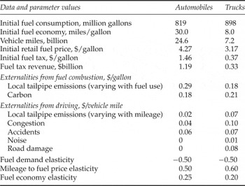
This section discusses how parameter values are obtained by pooling local data sources with extrapolations from US evidence and using judgment where data are unavailable. A later sensitivity analysis demonstrates that the valuation of health risks is the most important source of uncertainty, while alternative plausible assumptions for other parameters (e.g., fuel economy or emission rates) have relatively modest implications for corrective fuel taxes. Parameter values are for year 2006 or thereabouts and are summarized in table 1. All parameters are expressed in US currency (they can be converted into local currency using a market exchange rate of CLP 550 per US$ 1, the average rate that applied during 2006–2008).
Benchmark data and parameter assumptions (for year 2006 or thereabouts)

Source: See text and online appendix B for documentation.
3.1. Fuel use, prices and mileage data
Data are typically available for fuel use in the transportation sector, fuel prices and fuel taxes, but not for (nationwide) vehicle miles of travel or on-road fuel economy. However, if a plausible assumption about fuel economy can be made, mileage is easily inferred. We assume that the fuel economy of the existing automobile fleet in Chile is 30 miles per gallon, that is, somewhere between fuel economy in the United States (where there are a large proportion of relatively fuel-inefficient minivans, SUVs and pick-up trucks) and Europe. For heavy trucks, we assume fuel economy is 8 miles per gallon, based on US figures for single-unit trucks in Parry (Reference Parry2008, table 2). For 2007, total gasoline and diesel fuel consumption in Chile was 819 and 898 million gallons, respectively, with Santiago accounting for 46.7 and 39.7 per cent of these totals, respectively (SII, 2008).
Initial retail fuel prices for 2006 are taken to be $4.27/gallon for gasoline and $3.17/gallon for diesel, and the respective excise taxes are $1.46 and $0.37/gallon (SII, 2008). Fuels are also subject to value added taxes (VAT). However, VAT does not count towards the optimal fuel tax as it raises the price of goods in general rather than just fuels.
3.2. External damages from local tailpipe emissions
For regions outside Santiago, there are no local data on local pollution damages from automobiles. However, we believe it is reasonable for a first pass to extrapolate local pollution damages from the United States, after adjusting for differences in the value of statistical life (VSL) – given that damages are heavily dominated by mortality effects – and in vehicle emission rates. This procedure is described in online appendix B – based on an assumed VSL of $1.6 million for Chile, extrapolated from US VSL estimates – and the end result is damages of $0.007/mile.
For Santiago, we might expect much larger damages, given its high population density and that meteorological and topographical conditions are especially favorable to pollution formation. Rizzi (Reference Rizzi2008) provides detailed local evidence on pollution–health impacts for Santiago, based on a Chilean study (Cifuentes, Reference Cifuentes2001) of mortality and morbidity related to particulate matter (PM) and ozone exposure in Santiago in the late 1990s. From this evidence, we compute damage estimates of $0.06 per mile (online appendix B). Weighting damages for Santiago and the rest of the country by the respective mileage shares (assumed to be the same as the fuel consumption shares) gives a nationwide pollution cost of $0.03 per mile for Chile. As noted above, we apportion two-thirds of this cost to mileage and one-third to fuel use, to obtain the figures in table 1.
Based on our own calculations for Santiago (see online appendix B), we assume pollution damage costs for trucks, on a per-mile basis, are 3.4 times those for cars. This is consistent with relative car/truck damage estimates for the United States (FHWA, 2000, table 13).
3.3. Global pollution
Combusting a gallon of gasoline and diesel fuel produces 0.009 and 0.010 tons of CO2 respectively.Footnote 7 Worldwide damages from the future global warming potential of these emissions (e.g., from agricultural impacts, defense against sea level rise, health effects from the possible spread of tropical disease, damage risks from more extreme climate scenarios) are highly contentious. This reflects different views on the appropriate discount rate, the handling of low-probability/extreme damage outcomes, the valuation of ecosystem damage, and so on. Nonetheless, we think it is reasonable to follow a thorough assessment of available evidence by multiple US government agencies (US IAWG, 2010). They recommended a central damage value of US$ 21 per ton of CO2 for 2010 emissions (in year 2007 $) with low and high cases (which we use for sensitivity analysis) of $5 and $65 per ton.
3.4. Congestion
Marginal congestion costs depend on the marginal delay (i.e., the increase in delay to other road users due to the added congestion caused by one extra vehicle mile) and the value of travel time (VOT).
An approximation for the marginal delay (averaged across a region) can be inferred from data on average delay, and an assumption about the functional relation between marginal and average delay implied by speed/traffic flow curves (e.g., Lindsey and Verhoef, Reference Lindsey, Verhoef, Button and Hensher2000; Small and Verhoef, Reference Small and Verhoef2007, chapter 3). For Santiago, we obtain an estimate of average delay at peak and off-peak periods, by comparing observed travel speeds with speed under free-flow conditions, and we obtain marginal delay from average delay using the ‘Bureau of Public Roads’ speed/flow relation, which is widely used in traffic engineering models. As detailed in online appendix B, this procedure yields a marginal delay for Santiago of 0.035 hours per auto mile (averaged across time of day).
As for the rest of Chile, we assume no congestion in rural areas. For other urban centers we assume average travel speeds (with a shorter rush hour duration) are comparable to those outside the (congested) downtown core in Santiago. Reasonable information on these speeds is available from a local transportation model for Santiago and, based on these data, marginal delays in other cities are calculated at 32 per cent of those for Santiago as a whole. Weighting regional marginal delays by respective nationwide mileage shares yields marginal delay of 0.022 hours per mile, averaged across the nation (see online appendix B).
As for the VOT, we use a central value of $2.7 per hour and a range of $1.5–4.5 per hour for sensitivity analysis. The central figure is obtained by extrapolating evidence on the VOT for the United States, while the low end of the range encompasses current government practice in Chile and the upper end encompasses some evidence from local studies (see online appendix B).
Combining our central VOT and marginal delay yields a marginal external congestion cost of $0.06 per mile. One further complication is that driving on relatively congested roads (which are heavily used by commuters) is typically less sensitive to gasoline prices than driving on relatively uncongested roads. Thus, the congestion benefits from a given reduction in nationwide mileage are smaller than they would be if driving on congested and uncongested roads were equally price sensitive. Based on typical estimates of the relative sensitivity of driving under congested and uncongested conditions, Parry and Small (Reference Parry and Small2005) scaled back nationwide marginal congestion costs by 30 per cent. We follow the same procedure to obtain a preferred marginal external congestion cost of $0.04 per mile.
Finally, based on estimates from the literature (e.g., Santos and Fraser, Reference Santos and Fraser2006; Santos, Reference Santos2008), we assume that a vehicle mile by a heavy truck contributes 2.5 times as much to congestion as an extra car mile. These estimates take into account the extra road space used by trucks and their slower driving speeds, offset by their greater propensity for off-peak travel.
3.5. Accidents
Local data on traffic injuries are critical for gauging accident externalities, not least because the incidence of pedestrian/cyclist injuries – a major determinant of externalities – varies dramatically across countries (Kopits and Cropper, Reference Kopits and Cropper2008). As discussed in online appendix B, we start with Chilean accident data for various non-fatal injury classifications, for 2006. We make assumptions about what portion of personal injury, medical costs and property damages associated with these injuries are external (e.g., occupant injury risk in single vehicle collisions is assumed internal). The external components are then monetized using a mixture of local evidence and US extrapolations.
The end result is external cost for a car of $0.06 per mile. Pedestrian/ cyclist fatalities alone account for about three-quarters of this figure, therefore alternative assumptions about the extent to which medical costs, property damages and injuries in multi-vehicle collisions are external vs. internal have a relatively modest impact on the external cost estimate.
As for trucks, we follow FHWA (2000), de Palma et al. (Reference de Palma, Kilani and Lindsey2008) and Parry (Reference Parry2008) in assuming that external accident costs are 25 per cent greater than for cars, implying an externality of $0.07 per mile.Footnote 8
3.6. Road damage and noise
Road damage costs for trucks are estimated at $0.08 per mile and noise costs at a much smaller $0.01 per mile. Online appendix B provides details of these calculations. Road damage is inferred from government expenditures on road maintenance, after attributing a portion of these costs to other vehicles and other factors, while noise costs are obtained from US estimates (after making an adjustment for income and the share of urban vs. rural driving).
3.7. Elasticities
According to reviews by Glaister and Graham (Reference Glaister and Graham2002) and Goodwin et al. (Reference Goodwin, Dargay and Hanly2004), the long-run gasoline demand elasticity for countries like the United States is around −0.6, though a recent, widely cited study by Small and Van Dender (Reference Small and Van Dender2006) suggests a somewhat smaller size elasticity of −0.4. About 40 or 50 per cent of the elasticity is attributed to reduced mileage, as opposed to long-run vehicle fuel economy improvements. Given the wider availability of transit alternatives, we might expect mileage to be moderately more price responsive in Chile than in the United States.Footnote 9 We choose a value of −0.5 for the gasoline price elasticity, with the assumed response split equally between improved fuel economy and reduced driving.
The limited evidence available on diesel fuel elasticities for heavy trucks for high-income countries suggests that they are roughly comparable in magnitude to gasoline demand elasticities (e.g., Dahl, Reference Dahl1993: 122–123). It seems plausible that the mileage component of the elasticity is somewhat larger for diesel than for gasoline, as technological opportunities for improving fuel economy are more limited for trucks than for cars, given the high power requirements necessary to move freight. We use a diesel fuel price elasticity of −0.5, with 60 per cent of the response from changes in mileage, and 40 per cent from changes in fuel economy.
4. Corrective fuel tax calculations
4.1. Benchmark results
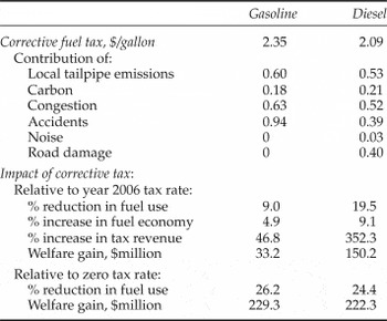
The top half of table 2 presents the corrective tax calculations under our benchmark parameter assumptions.
Corrective tax computations: benchmark parameter values (year 2006 US$)

Source: See text for formulas and parameter assumptions underlying these calculations.
4.1.1. Gasoline tax
The corrective gasoline tax is $2.35 per gallon, which is 60 per cent larger than the rate prevailing in 2006. Traffic accidents account for 40 per cent of the tax, congestion 27 per cent, local tailpipe emissions 26 per cent, and global warming 8 per cent.
This corrective tax estimate is higher than comparable estimates for the United States (e.g., Parry and Small, Reference Parry and Small2005). At first glance, this seems surprising given the lower valuation of health risks and travel time in Chile. However, one offsetting factor is that accident externalities are much larger in Chile, due to the much higher incidence of pedestrian/cyclist fatalities. In addition, despite the lower VOT in Chile, our nationwide figure for marginal congestion costs is comparable to that in US studies, because a larger share of nationwide driving occurs under highly congested conditions (in Santiago). Similarly, although the assumed VSL for Chile is lower, the (nationwide) pollution-mortality rate is greater, given the large share of the population residing in Santiago and therefore being exposed to elevated risks. Yet another factor is that the assumed miles per gallon is larger in Chile than the United States. This implies a greater reduction in mileage per gallon of fuel saved, which in turn magnifies the mileage-related externality benefits, particularly congestion and accidents (through lowering g in equation (2a)).
4.1.2. Diesel tax
The corrective diesel fuel tax in the benchmark case is $2.09 per gallon. This is smaller than the corrective gasoline tax, but only moderately so – external cost considerations do not warrant the current, and strikingly large, tax preference for diesel over gasoline.
Local and global pollution contribute a roughly similar amount to the corrective tax for either fuel. However, unlike for gasoline, road damage contributes a significant amount ($0.40 per gallon) to the diesel tax (the contribution from noise is small). On the other hand, an offsetting factor is that trucks travel a shorter distance on a gallon of fuel than cars, which substantially reduces the mileage-related externalities per gallon of diesel fuel reduction. This is particularly the case for accidents, which contribute 39 cents to the corrective diesel tax compared to 94 cents for the corrective gasoline tax. Congestion also contributes less, but only moderately so (52 cents to the diesel tax and 63 cents to the gasoline tax), given our assumption that a truck mile contributes two-and-a-half times the congestion a car mile does. Again, this corrective tax estimate is higher than for comparable estimates for the United States (e.g., Parry, Reference Parry2008), for broadly similar reasons to those for the gasoline tax.
4.1.3. Impacts of tax reform
Also indicated in the lower half of table 2 is the impact of tax reform. Raising taxes from their 2006 levels to their corrective levels in the benchmark case would reduce (long-run) gasoline and diesel use by an estimated 9.0 and 19.5 per cent respectively (the latter reduction is much larger due to the much larger difference between corrective and initial tax rates). The fuel economy increase is 4.9 per cent for cars and 9.1 per cent for trucks. Under corrective taxes, gasoline tax revenue increases 47 per cent above 2006 levels while diesel tax revenues are 3.5 times as large. Annual welfare gains from raising taxes on gasoline and diesel to their corrective levels are $33.2 million and $150.2 million, respectively.
If initial tax rates were zero (and initial fuel consumption were proportionately larger according to equation (4)), fuel reductions from implementing the corrective tax would be in the order of 25 per cent for either fuel. Estimated welfare gains (from the corrective fuel tax relative to no tax) would be substantially larger at $229 million and $222 million, respectively.
4.2. Sensitivity analysis
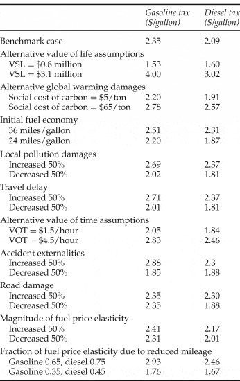
Table 3 indicates corrective fuel taxes under a wide range of alternative parameter scenarios (where parameters are varied one at a time).
Corrective tax calculations: alternative parameter values

Results are most sensitive to the VSL. As discussed in online appendix B, a plausible range of values for the Chilean VSL could be anywhere from about $0.8 to $3.1 million. Using the higher VSL almost doubles local pollution and accident externalities and the corrective gasoline and diesel taxes increase to $4.00 per gallon and $3.02 per gallon respectively. On the other hand, under the low VSL value the corrective gasoline and diesel taxes fall to $1.53 per gallon and $1.60 per gallon, respectively. In the remaining cases in table 3, alternative parameter assumptions can have significant, but less dramatic, effects on corrective fuel taxes.
Using a higher value for global warming damages – $65 per ton of CO2 instead of $21 per ton – increases the corrective gasoline tax and diesel tax by $0.43 and $0.48 per gallon, respectively.
We vary the initial fuel economy between 24 and 36 miles per gallon for cars and between 6.4 and 9.6 miles per gallon for trucks. This causes the corrective fuel taxes to vary by about ±6 per cent for cars and ±10 per cent for trucks as higher (lower) fuel economy magnifies (dampens) the contribution of mileage-related externalities.
Increasing and decreasing local pollution damages by up to 50 per cent causes the corrective fuel taxes to vary by up to about ±14 per cent, while increasing and decreasing marginal travel delay by up to 50 per cent causes corrective taxes to vary by up to about ±15 per cent. Using the smaller value for the VOT ($1.50 instead of $2.70 per hour) decreases both corrective taxes by about 12 per cent. Varying accident externalities by ±50 per cent causes the corrective gasoline tax to vary by about ±20 per cent and the corrective diesel tax to vary between about ±10 per cent. Varying road damage ±50 per cent causes the corrective diesel tax to vary between ±10 per cent.
The results are fairly insensitive to varying own-price fuel elasticities, with mileage and fuel economy elasticities changing in the same proportion. More significant is, for a given overall fuel price elasticity, the relative price responsiveness of mileage and fuel economy (which determines β and α in equations (2) and (6)). As indicated in the last row of table 3, varying the fraction of the gasoline elasticity that is due to reduced mileage from 0.35 to 0.65 causes the corrective gasoline tax to vary between about ±25 per cent. And varying the fraction of the diesel fuel price elasticity due to mileage between 0.45 and 0.75 causes the corrective diesel tax to vary between approximately ±20 per cent.
5. Conclusion
This paper presents a methodology for compiling estimates of parameters needed to assess corrective motor fuel taxes for a middle-income country. We use Chile as an illustration, although we believe the paper provides a useful template for approximately gauging corrective fuel taxes in other countries at similar levels of development (at least those with comparable data sources).
For Chile, the corrective gasoline and diesel taxes are $2.35 and $2.09 per gallon in the benchmark case – higher than typical tax rates prevailing in western hemisphere countries, but lower than typical rates in western Europe. Despite lower valuations of health risks and travel delays, the corrective fuel tax estimates for Chile are larger than comparable estimates for the United States. This is due to a mix of factors, including the higher incidence of pedestrian fatalities in Chile as well as the high proportion of its population residing and driving in the metropolitan Santiago region, where conditions are conducive to pollution formation and roads are clogged.
Again, we emphasize that the analysis is only meant to provide a first-pass assessment. There is plenty of scope for parameter estimates to improve with better data although, aside from the (contentious) valuation of mortality risk, we conjecture that, in most cases, refinements will likely have a non-dramatic impact on corrective fuel tax estimates.
Another caveat is that there are far more efficient instruments than fuel taxes for addressing some of the key externalities. Traffic congestion is better addressed through per-mile tolls on congested roads that rise and fall during the course of the rush hour (e.g., Santos, Reference Santos2004). These taxes would exploit all of the possible behavioral responses for reducing congestion – encouraging people to commute earlier or later to avoid the peak of the rush hour, to car pool, to use public transport rather than drive, to reduce their overall number of trips, to relocate jobs out of busy downtown areas, etc. Accident externalities can be efficiently reduced through a transition to pay-as-you drive auto insurance (Bordhoff and Noel, Reference Bordoff and Noel2008). Under this approach, a driver's insurance payment is the product of their annual miles driven and a per-mile charge that depends on their risk factor (as determined by their age, prior crash record, etc.) so drivers with greatest accident risk have most incentive to conserve on vehicle use. However, until congestion and accident externalities are comprehensively internalized through other instruments, in the interim it is entirely appropriate to include them in fuel tax assessment.Footnote 10
Our analysis abstracts from linkages between fuel taxes and the broader fiscal system, particularly tax distortions in the labor market which depress the level of work effort below economically efficient levels. These interactions take two forms (e.g., Goulder, Reference Goulder1995). First is the potential efficiency gain from using fuel tax revenues to reduce distortionary taxes, or fund socially productive public projects. Second is an efficiency loss to the extent that higher transportation prices cause a (slight) contraction in economic activity and hence labor supply. For the United States, West and Williams (Reference West and Williams2007) find evidence that the former effect exceeds the latter – in other words, gasoline is a relatively weak substitute for leisure – implying that the optimal (revenue-neutral) tax is somewhat higher than the corrective tax. However, reliable evidence on labor supply responses to income and fuel taxes, which is needed to make these types of adjustments to optimal fuel tax estimates for Chile, is not available at present.
Finally, the distributional argument against higher fuel taxes in Chile seems open to question given that, according to CASEN (2006), in 2006 only 9.4 per cent of households in the bottom income decile owned a car, compared with 72.7 per cent for the top-income decile. Furthermore, it could be argued that holding down fuel taxes below levels warranted on externality grounds is an inefficient way to help poor households, as this benefits all households, not just the target group. In general, distributional goals are better met through more targeted provisions in the tax and benefit system, education policy, housing policy, and so on.