1. Introduction
Roughness plays an important role in many fields of study. A substantial amount of work has been carried out to understand the dynamics of turbulent flows over rough walls, both for engineering and atmospheric applications. Roughness effects on the flow are summarized by Raupach, Antonia & Rajagopalan (Reference Raupach, Antonia and Rajagopalan1991) and Jiménez (Reference Jiménez2004). Roughness increases the drag on the wall due to the pressure drag, resulting from the wake created downstream of a roughness element. Many studies have shown that, far away from the wall, roughness does not affect the turbulent statistics, but it sets the velocity scale by increasing the friction coefficient.
Inside the roughness sublayer (defined as the region where roughness causes spatial variations of time-averaged turbulent statistics), the flow dynamics is significantly altered as the turbulent structures become more three-dimensional. In order to capture the interaction between the turbulence and the spatial variation of the time-averaged velocity field (wake), the space–time double-averaging (DA) approach can be used (Raupach & Shaw Reference Raupach and Shaw1982). Earlier studies of flow over canopies (Raupach et al. Reference Raupach, Antonia and Rajagopalan1991; Finnigan Reference Finnigan2000) found that the wake leads to an additional source term in the budget of the turbulent kinetic energy (TKE) – the ‘wake production’.
Roughness and sediments are different from canopies in the vertical distribution of the density of the roughness elements. Recent studies on flow over gravel beds (Mignot, Bartheleemy & Hurther Reference Mignot, Bartheleemy and Hurther2009; Dey & Das Reference Dey and Das2012) found that the effect of the wake on TKE is negligible compared to the production due to the shear of the mean velocity (shear production).
Direct and large-eddy simulations have studied the roughness effects on wall-bounded flows, e.g. Kanda, Moriwaki & Kasamatsu (Reference Kanda, Moriwaki and Kasamatsu2004), Coceal et al. (Reference Coceal, Thomas, Castro and Belcher2006), Orlandi & Leonardi (Reference Orlandi and Leonardi2008), Leonardi & Castro (Reference Leonardi and Castro2010) and Lee, Sung & Krogstad (Reference Lee, Sung and Krogstad2011). Their main focus has been on the flow above the roughness and the parameterization of the drag. The layer below the roughness crest, however, is also important; understanding this layer would provide insights into the roughness effects in the regions above. It was observed by Coceal et al. (Reference Coceal, Thomas, Castro and Belcher2006) that the wake depends on the geometry of the roughness, and that, although smaller than the Reynolds stresses, the dispersive stresses (resulting from the wake component) are significant in the lower part of the roughness sublayer. However, the effects of roughness on the budgets of specific Reynolds normal stresses have not been well studied. It is important to understand the effects of roughness on the wall-normal and spanwise turbulent fluctuations, since these two components are more direct indicators (than TKE) of inner–outer-layer interactions, near-wall structure instability and drag generation. To this end, we use direct numerical simulations (DNS) of the turbulent flow over sandgrain roughness in the transitionally and fully rough regimes to study the roughness effects on the budgets of the Reynolds stresses, and to investigate the energy transfer between the wake and the turbulence.
2. Problem formulation
2.1. Governing equations and numerical techniques
The incompressible flow of a Newtonian fluid is governed by the equations of conservation of mass and momentum,
 $$\begin{eqnarray}\displaystyle & \displaystyle \frac{\partial u_{i}}{\partial x_{i}}=0, & \displaystyle\end{eqnarray}$$
 $$\begin{eqnarray}\displaystyle & \displaystyle \frac{\partial u_{i}}{\partial t}+\frac{\partial u_{i}u_{j}}{\partial x_{j}}=-\frac{\partial P}{\partial x_{i}}+{\it\nu}\frac{\partial ^{2}u_{i}}{\partial {x_{j}}^{2}}+F_{i}, & \displaystyle\end{eqnarray}$$
where
 $u_{i}$
and
 $P$
are the velocities and pressure.
Here
 $x_{1}$
,
 $x_{2}$
and
 $x_{3}$
(or
 $x$
,
 $y$
and
 $z$
) are, respectively, the streamwise, wall-normal and spanwise directions, and
 $u_{i}$
(or
 $u$
,
 $v$
and
 $w$
) are the velocity components in those directions;
 $P=p/{\it\rho}$
is the modified pressure,
 ${\it\rho}$
the density and
 ${\it\nu}$
the kinematic viscosity. We performed DNS of (2.1) and (2.2) using a staggered grid and second-order central differences for all terms, a second-order semi-implicit time advancement, and message passing interface (MPI) parallelization (Keating et al.
Reference Keating, Piomelli, Bremhorst and Nešić2004). An immersed-boundary method (IBM) based on the volume-of-fluid approach (Scotti Reference Scotti2006; Yuan & Piomelli Reference Yuan and Piomelli2014) is applied: a body force,
 $F_{i}$
, is used to impose the no-slip boundary condition on the rough surfaces; it is non-zero in the interface cell only. Details of the model can be found in Yuan & Piomelli (Reference Yuan and Piomelli2014).
2.2. Averaging approach
Following Mignot et al. (Reference Mignot, Bartheleemy and Hurther2009), a DA approach is applied to decompose a flow quantity,
 ${\it\theta}$
, into the space–time average,
 $\langle \overline{(\cdot )}\rangle$
(bar and brackets denote temporal and spatial averages, respectively), the spatial disturbance of the temporal average,
 $\widetilde{(\cdot )}$
, and the turbulent fluctuation (denoted by the prime),
 $$\begin{eqnarray}{\it\theta}(x,y,z,t)=\langle \overline{{\it\theta}}\rangle (y)+\widetilde{{\it\theta}}(x,y,z)+{\it\theta}^{\prime }(x,y,z,t).\end{eqnarray}$$
Two spatial averaging approaches are used (Nikora et al.
Reference Nikora, McEwan, McLean, Coleman, Pokrajac and Walters2007). The intrinsic spatial average,
 $\langle \cdot \rangle$
, is carried out in the
 $(x,z)$
-plane, in the fluid domain only, while the superficial average,
 $\langle \cdot \rangle _{s}$
, is carried out over the whole
 $(x,z)$
-plane.
Applying the intrinsic average to the time-averaged
 $u$
-momentum equation for the open-channel flow, one obtains
 $$\begin{eqnarray}-\left\langle \frac{\partial \overline{P}}{\partial x}\right\rangle +{\it\nu}\left\langle {\rm\nabla}^{2}\overline{u}\right\rangle -\left\langle \frac{\partial \overline{u}\,\overline{v}}{\partial y}\right\rangle -\left\langle \frac{\partial \overline{u^{\prime }v^{\prime }}}{\partial y}\right\rangle =0.\end{eqnarray}$$
Note that the IBM force
 $F_{i}$
does not appear in (2.4) since it is zero inside the fluid domain. Equation (2.4) can be written as
 $$\begin{eqnarray}-\frac{\partial \langle \overline{P}\rangle _{s}}{\partial x}+{\it\nu}\frac{\partial ^{2}\langle \overline{u}\rangle _{s}}{\partial y^{2}}-\frac{\partial \langle \overline{u^{\prime }v^{\prime }}\rangle _{s}}{\partial y}-\frac{\partial \langle \widetilde{u}\,\widetilde{v}\rangle _{s}}{\partial y}-\left\langle \frac{\partial \widetilde{P}}{\partial x}\right\rangle _{s}+{\it\nu}\langle {\rm\nabla}^{2}\widetilde{u}\rangle _{s}=0,\end{eqnarray}$$
where the last two terms on the left-hand side are, respectively, the pressure drag,
 $f_{p}$
, and the viscous drag,
 $f_{{\it\nu}}$
(Raupach & Shaw Reference Raupach and Shaw1982); they arise due to the non-commutativity between the operators
 $\partial /\partial x_{i}$
and
 $\langle \cdot \rangle$
below the roughness crest. The sum of these two terms is the total drag. It can be shown that
 $F_{1}$
, averaged in the interface cell in the
 $(x,z)$
-plane, equals the total drag,
 $-\langle \partial \widetilde{P}/\partial x\rangle _{s}+{\it\nu}\langle {\rm\nabla}^{2}\widetilde{u}\rangle _{s}$
.
2.3. Simulation parameters
An open-channel flow of domain size
 $6h\times 1h\times 3h$
in
 $x$
,
 $y$
and
 $z$
is simulated; this size is sufficient to accommodate the largest turbulent structures on a smooth-wall channel flow. No-slip and symmetric boundary conditions are applied to the bottom wall and to the top boundary, respectively. Periodic conditions are used in both the
 $x$
and
 $z$
directions. A constant pressure gradient is applied to drive the flow. A virtual sandgrain model (Scotti Reference Scotti2006) is used to impose roughness at the bottom boundary: the bottom domain is separated into tiles of approximate size
 $2k_{s}\times 2k_{s}$
; a roughness element is planted in each tile, which constitutes a randomly rotated ellipsoid with semi-axes equalling
 $k_{s}$
,
 $1.4k_{s}$
and
 $2k_{s}$
. Note that, for this virtual sandgrain surface,
 $k_{s}$
is known a priori since the model is calibrated, in a specific range of roughness Reynolds numbers, to give the same roughness function as the Nikuradse sandgrain with a height
 $k_{s}$
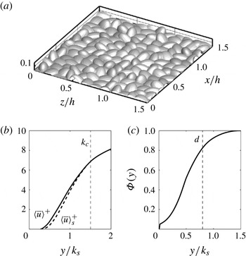
; however, the shape of the elements is not exactly the same as those of Nikuradse. A fraction of the surface is visualized in figure 1(a) as an iso-surface of the fluid volume fraction equalling 0.5. The Reynolds number based on the half-channel height (
 $h$
) and the friction velocity (
 $u_{{\it\tau}}$
) is
 $\mathit{Re}_{{\it\tau}}=1000$
. Two roughness heights are used to yield a transitionally rough and a fully rough flow: a low-roughness case (R1,
 $k_{s}/h=0.02$
,
 $k_{s}^{+}=22$
) and a high-roughness case (R2,
 $k_{s}/h=0.07$
,
 $k_{s}^{+}=72$
). The roughness crests (
 $k_{c}$
) for R1 and R2 are 3 % and 9 % of
 $h$
, respectively. A smooth-wall case (case SM) is also included for comparison.
(a) Visualization of an eighth of the surface R2. Wall-normal profiles of (b) DA streamwise velocity (——,
 $\langle \overline{u}\rangle$
; - - - -,
 $\langle \overline{u}\rangle _{s}$
) and (c) roughness geometry function.

Table 1 tabulates the parameters and spatial resolutions. Uniform grids are used in the
 $x$
and
 $z$
directions, while the grid is refined near the wall in the
 $y$
direction. For the rough cases,
 ${\rm\Delta}y^{+}<1$
for
 $y\leqslant k_{c}$
, resulting in more than 31 and 51 grid points in
 $y$
below the mean roughness height and the crest, respectively. For the smooth case,
 ${\rm\Delta}y_{min}^{+}=0.3$
, with four points below
 $y^{+}=1$
. The total number of grid points varies between 70 and 130 million. The grid sizes in the
 $x$
and
 $z$
directions are less than or equal to 12 and 6 wall units, respectively, which is sufficient for DNS resolution.
Parameters for all cases.
 $k_{c}$
is the roughness crest;
 $\overline{k}$
is the mean roughness height.
 $n_{j}$
ranges from 128 to 256.
 $N_{x_{i}}$
: grid points per sandgrain element.

The shape resolution of a roughness element is quantified by
 $N_{x_{i}}$
, the number of grid points (in
 $x_{i}$
) used to resolve the shape of each sandgrain element. A grid-convergence study (not shown) was carried out, and it was found that the present resolution is sufficient to obtain the Reynolds stresses and their budgets. For all cases, data are collected from a total simulation time of
 $T=50h/u_{{\it\tau}}$
after the transient. A convergence study showed that decreasing the simulation time to
 $0.5T$
leads to errors of less than 1 % for third-order (or lower) turbulent statistics.
3. Results
3.1. Turbulent statistics
The DA streamwise velocity is shown in figure 1(b). Below the roughness crest, the velocity varies almost linearly, consistent with Model III of the velocity distribution proposed by Nikora et al. (Reference Nikora, Koll, McEwan, McLean and Dittrich2004) applied to rough-wall flows with relatively low submergence (
 $h/k_{s}$
). The superficial average (
 $\langle \overline{u}\rangle _{s}={\it\Phi}\langle \overline{u}\rangle$
) is lower than the intrinsic average, since the roughness geometry function,
 ${\it\Phi}(y)$
, defined as the fraction of space occupied by fluid in the horizontal plane at
 $y$
, is less than one (figure 1
c). The distribution of
 ${\it\Phi}(y)$
is not affected by the variation of the spatial resolution. The zero-plane displacement (d), representing the effective elevation of the boundary layer due to roughness, is obtained as the location of the centroid of the wall-normal averaged drag-force profile (Yuan & Piomelli Reference Yuan and Piomelli2014);
 $d\approx 0.8k_{s}$
for both rough cases.
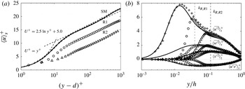
Figure 2(a) shows the DA velocity profiles in wall units. The roughness functions,
 ${\rm\Delta}U^{+}$
, obtained as the offsets of
 $\langle \overline{u}\rangle _{s}^{+}$
profiles in the logarithmic region from the universal logarithmic law, are 3.5 and 7.8 for cases R1 and R2, respectively, yielding
 $k_{s}^{+}=22$
and 72 based on the Colebrook correlation (Colebrook Reference Colebrook1939); case R2 is in the fully rough regime, while case R1 is transitionally rough.
(a) Streamwise velocity and (b) Reynolds stresses for cases SM (——), R1 (○) and R2 (▵).
 $+$
represents the smooth-wall experiment (Schultz & Flack Reference Schultz and Flack2013).
 $k_{R}$
: top of the roughness sublayer.

The Reynolds stresses in cases R1 and R2 are compared in figure 2(b) with smooth-wall experimental data from channel-flow studies with the same Reynolds number (Schultz & Flack Reference Schultz and Flack2013); agreement is obtained in the outer layer, supporting the wall similarity hypothesis. Case R1 preserves a high near-wall peak of the streamwise normal Reynolds stress, while the peak is significantly damped for case R2, due to the destruction of the buffer layer. The top of the roughness sublayer is denoted by
 $k_{R}$
; its location will be discussed below. Inside the roughness sublayer, all normal Reynolds stresses in wall units are damped, compared to case SM. The magnitudes of the other two shear stresses are negligible compared to
 $\langle \overline{u^{\prime }v^{\prime }}\rangle$
, due to the randomness of the rough surface.
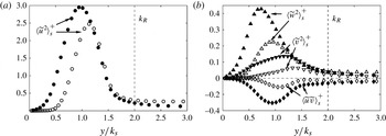
The form-induced (or dispersive) stresses are shown in figure 3 for both rough cases; the wall-normal and spanwise components are smaller than the corresponding components of the Reynolds stresses, consistent with previous experimental rough-wall and canopy studies (Nikora et al.
Reference Nikora, Goring, McEwan and Griffiths2001; Mignot et al.
Reference Mignot, Bartheleemy and Hurther2009); the streamwise form-induced stress is comparable to the Reynolds stress, a characteristic of relatively low submergence (Manes, Pokrajac & McEwan Reference Manes, Pokrajac and McEwan2007). The peak of
 $|\langle \widetilde{u}\,\widetilde{v}\rangle _{s}^{+}|$
is around 0.15, consistent with a previous DNS study by Coceal et al. (Reference Coceal, Thomas, Castro and Belcher2006). The region with non-negligible
 $\langle \widetilde{u}_{i}^{2}\rangle _{s}$
is the roughness sublayer, whose thickness,
 $k_{R}$
, is shown to be around
 $2k_{s}$
. The magnitude of the form-induced stresses relative to the Reynolds stresses increases with
 $k_{s}^{+}$
, since, in the roughness sublayer,
 $\langle \overline{u_{i}^{\prime 2}}\rangle ^{+}$
decreases while
 $\langle \widetilde{u}_{i}^{2}\rangle ^{+}$
increases with higher
 $k_{s}^{+}$
, due to the lower submergence.
Form-induced stresses for cases R1 (empty symbols) and R2 (filled symbols): (a)
 $\langle \widetilde{u}^{\,2}\rangle _{s}^{+}$
; (b) ▿,
 $\langle \widetilde{v}^{\,2}\rangle _{s}^{+}$
; ▵,
 $\langle \widetilde{w}^{\,2}\rangle _{s}^{+}$
; ♢,
 $\langle \widetilde{u}\,\widetilde{v}\rangle _{s}^{+}$
.

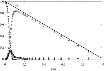
Figure 4 shows the stress balance for case R2; the mean pressure gradient is balanced by the sum of the other stresses,
 $$\begin{eqnarray}{\it\tau}^{+}=\int _{y^{+}}^{h^{+}}(f_{{\it\nu}}^{+}+f_{p}^{+})\text{d}y^{+}-\langle \overline{u^{\prime }v^{\prime }}\rangle _{s}^{+}+\frac{\partial \langle \overline{u}\rangle _{s}^{+}}{\partial y^{+}}-\langle \widetilde{u}\,\widetilde{v}\rangle _{s}^{+}=1-\frac{y^{+}}{h^{+}}.\end{eqnarray}$$
The viscous stress is small, consistent with fully rough flow. The form-induced shear stress is also small compared to the Reynolds shear stress. The total drag,
 $(\,f_{{\it\nu}}^{+}+f_{p}^{+})$
, calculated from momentum balance, agrees with the IBM force,
 $\langle F_{1}\rangle _{s}$
, which can be used to calculate the total drag, as shown by Yuan & Piomelli (Reference Yuan and Piomelli2014).
Stress balance of case R2. ——, total stress from momentum balance; ▵, total drag from momentum balance; - - - -, total drag from the
 $F_{1}$
integral; ▫, Reynolds shear stress; ○, form-induced shear stress;
 $+$
viscous stress due to mean shear.

3.2. Budgets of Reynolds and dispersive stresses
In the turbulent flow over roughness, the total kinetic energy can be decomposed into three parts,
 $$\begin{eqnarray}{\textstyle \frac{1}{2}}\langle \overline{u_{i}u_{i}}\rangle ={\textstyle \frac{1}{2}}\langle \overline{u}_{i}\rangle \langle \overline{u}_{i}\rangle +{\textstyle \frac{1}{2}}\langle \widetilde{u}_{i}\widetilde{u}_{i}\rangle +{\textstyle \frac{1}{2}}\langle \overline{u_{i}^{\prime }u_{i}^{\prime }}\rangle ,\end{eqnarray}$$
where the terms on the right-hand side are, respectively, the mean-flow kinetic energy (MKE), the WKE and the TKE. The MKE is converted to small-scale TKE (and consequently heat) in two ways (Finnigan Reference Finnigan2000): first, the energy goes through the whole energy cascade; second, MKE first generates WKE of scale
 $k_{s}$
due to the work of the mean flow against the total drag, and the WKE generates TKE of scales smaller than
 $k_{s}$
through the energy cascade, called ‘short-circuited’ cascade by Raupach et al. (Reference Raupach, Antonia and Rajagopalan1991). The interactions between WKE and TKE also take place in two ways: WKE generates TKE of scales smaller than
 $k_{s}$
, while TKE is converted to WKE through the work of large-scale turbulent structures against the form drag.
The budgets of Reynolds stresses and TKE were derived by Raupach & Shaw (Reference Raupach and Shaw1982) for flow over canopies and by Mignot et al. (Reference Mignot, Bartheleemy and Hurther2009) for flow over roughness. The budgets of the normal Reynolds stresses are (no summation over the Greek index)
 $$\begin{eqnarray}\displaystyle & & \displaystyle -2\langle \overline{u_{{\it\alpha}}^{\prime }v^{\prime }}\rangle \frac{\partial \langle \overline{u}_{{\it\alpha}}\rangle _{s}}{\partial y}-2\left\langle \widetilde{u_{{\it\alpha}}^{\prime }u_{j}^{\prime }}\frac{\partial \widetilde{u}_{{\it\alpha}}}{\partial x_{j}}\right\rangle _{s}-\frac{\partial }{\partial y}\langle \widetilde{u_{{\it\alpha}}^{\prime }u_{{\it\alpha}}^{\prime }}\widetilde{v}\rangle _{s}-\frac{\partial }{\partial y}\langle \overline{u_{{\it\alpha}}^{\prime }u_{{\it\alpha}}^{\prime }v^{\prime }}\rangle _{s}\nonumber\\ \displaystyle & & \displaystyle \quad -\,2\left\langle \overline{u_{{\it\alpha}}^{\prime }\frac{\partial P^{\prime }}{\partial x_{{\it\alpha}}}}\right\rangle _{s}+{\it\nu}\frac{\partial ^{2}}{\partial y^{2}}\langle \overline{u_{{\it\alpha}}^{\prime }u_{{\it\alpha}}^{\prime }}\rangle _{s}-{\it\epsilon}_{{\it\alpha}{\it\alpha}}=0.\end{eqnarray}$$
Summing over the three components yields the budget of the TKE,
 $$\begin{eqnarray}\displaystyle & & \displaystyle -\langle \overline{u_{i}^{\prime }v^{\prime }}\rangle \frac{\partial \langle \overline{u}_{i}\rangle _{s}}{\partial y}-\left\langle \widetilde{u_{i}^{\prime }u_{j}^{\prime }}\frac{\partial \widetilde{u}_{i}}{\partial x_{j}}\right\rangle _{s}-\frac{\partial }{\partial y}\langle \widetilde{u_{i}^{\prime }u_{i}^{\prime }}\widetilde{v}\rangle _{s}/2\nonumber\\ \displaystyle & & \displaystyle \quad -\,\frac{\partial }{\partial y}\langle \overline{u_{i}^{\prime }u_{i}^{\prime }v^{\prime }}\rangle _{s}/2-\frac{\partial }{\partial y}\langle \overline{P^{\prime }v^{\prime }}\rangle _{s}+{\it\nu}\frac{\partial ^{2}}{\partial y^{2}}\langle \overline{u_{i}^{\prime }u_{i}^{\prime }}/2\rangle _{s}-{\it\epsilon}_{k}=0,\end{eqnarray}$$
where the terms on the left-hand side are, respectively, shear production (
 $P_{s}$
), wake production (
 $P_{w}$
), transport due to wake, turbulent transport (
 $T_{t}$
), pressure transport (
 $T_{p}$
), viscous transport (
 $T_{{\it\nu}}$
) and viscous dissipation (
 ${\it\epsilon}$
).
 ${\it\epsilon}$
is obtained as the residual of the sum of all other terms. In the normal-stress budget the pressure work,
 ${\it\Pi}_{{\it\alpha}{\it\alpha}}$
, is also present.
The budget of WKE,
 $\langle \widetilde{u}_{i}\widetilde{u}_{i}\rangle /2$
, was derived by Raupach & Shaw (Reference Raupach and Shaw1982). Taking into account the vertically varying roughness geometry function,
 ${\it\Phi}(y)$
, the budgets of the normal dispersive stresses (
 $\langle \widetilde{u}_{{\it\alpha}}^{2}\rangle$
) read
 $$\begin{eqnarray}\displaystyle & & \displaystyle -2\langle \widetilde{u}_{{\it\alpha}}\widetilde{v}\rangle \frac{\partial \langle \overline{u}_{{\it\alpha}}\rangle _{s}}{\partial y}+2\left\langle \widetilde{u_{{\it\alpha}}^{\prime }u_{j}^{\prime }}\frac{\partial \widetilde{u}_{{\it\alpha}}}{\partial x_{j}}\right\rangle _{s}-\frac{\partial }{\partial y}\langle \widetilde{u}_{{\it\alpha}}\widetilde{u}_{{\it\alpha}}\widetilde{v}\rangle _{s}-2\frac{\partial }{\partial y}\langle \widetilde{u}_{{\it\alpha}}\widetilde{u_{{\it\alpha}}^{\prime }v^{\prime }}\rangle _{s}\nonumber\\ \displaystyle & & \displaystyle \quad -\,2\left\langle \widetilde{u}_{{\it\alpha}}\frac{\partial \widetilde{P}}{\partial x_{{\it\alpha}}}\right\rangle _{s}+2{\it\nu}\langle \widetilde{u}_{{\it\alpha}}{\rm\nabla}^{2}\widetilde{u}_{{\it\alpha}}\rangle _{s}=0,\end{eqnarray}$$
where the six terms on the left-hand side are, respectively, shear production of WKE, wake production (
 $-P_{w}$
), transport due to wake, transport due to turbulence, work done by pressure, and viscous diffusion and dissipation at the wake level.
The term
 $P_{w}$
appears with opposite signs in the budgets of TKE and WKE; it is the net transfer from WKE to TKE as the result of their interactions. Previous studies on flows above canopies found that
 $P_{w}$
is usually positive (WKE converts to TKE), with magnitudes comparable to
 $P_{s}$
(Raupach et al.
Reference Raupach, Antonia and Rajagopalan1991; López & García Reference López and García2001). In the experimental study of flow over gravel beds (Mignot et al.
Reference Mignot, Bartheleemy and Hurther2009), however, the magnitude of
 $P_{w}$
was found to be less than 5 % of
 $P_{s}$
.
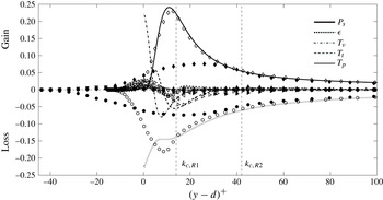
The TKE budgets normalized by wall units are shown in figure 5. Case SM has been validated with the smooth-wall channel-flow DNS results reported by Hoyas & Jiménez (Reference Hoyas and Jiménez2008) (not shown). Above the roughness sublayer (
 $y>k_{R}$
) the R1 budget terms agree well with case SM, while in the roughness sublayer they differ from the smooth case mainly in that, approaching the wall, both
 ${\it\epsilon}_{k}$
and
 $T_{{\it\nu}}$
become zero, indicating a quiet region without turbulence at the root of the roughness.
TKE budgets for cases SM (line), R1 (empty symbols) and R2 (filled symbols). All terms normalized by
 $u_{{\it\tau}}^{4}/{\it\nu}$
. - - - -
 $k_{c}$
, roughness crest. Symbols: ♢,
 $P_{s}$
; ▵,
 $P_{w}$
; ○,
 ${\it\epsilon}$
; ▹,
 $T_{t}$
; ◃,
 $T_{{\it\nu}}$
; ▿,
 $T_{p}$
. Note that the actual bottom-wall location varies.

Figure 5 also shows that, for both rough cases, the location of the peak of the shear production is close to the roughness crest, connected to the shear layers formed near the crest (Ikeda & Durbin Reference Ikeda and Durbin2007; Mignot et al.
Reference Mignot, Bartheleemy and Hurther2009). For case R2,
 $P_{s}$
peaks at
 $0.73k_{c}$
from the actual bottom wall (where
 ${\it\Phi}=0$
), while, for case R1, it peaks at
 $0.93k_{c}$
. It was observed by Mignot et al. (Reference Mignot, Bartheleemy and Hurther2009) that, for flow over gravel beds,
 $P_{s}$
peaks around
 $0.9k_{c}$
.
 $P_{s}$
decreases from its peak location to the virtual wall. Dissipation peaks slightly below the production peak; the transport terms are non-negligible in the roughness sublayer only. Both the turbulent diffusion and the viscous diffusion take energy from the region with high production (near
 $k_{c}$
) and transport it towards the wall to balance dissipation. These observations are consistent with the literature (Finnigan Reference Finnigan2000; Mignot et al.
Reference Mignot, Bartheleemy and Hurther2009; Hong, Katz & Schultz Reference Hong, Katz and Schultz2011). Furthermore, the pressure transport removes TKE from near the roughness crest, and transports it to the lower part of the roughness sublayer; for case R2, the pressure transport is the most important source term in the lowest third of the sublayer, consistent with large-eddy simulation results in flow within forest canopies (Dwyer, Patton & Shaw Reference Dwyer, Patton and Shaw1997), while in the transitionally rough case R1, the viscous diffusion is the most important source term in the lowest part of the sublayer. Compared to
 $P_{s}$
and
 ${\it\epsilon}$
,
 $P_{w}$
is much smaller, consistent with Mignot et al. (Reference Mignot, Bartheleemy and Hurther2009). The sign and magnitude of
 $P_{w}$
are affected by the roughness height, as will be explained later.
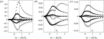
Selected terms of the normal Reynolds stress budgets (in wall units) are shown in figure 6. The wall-normal distance is normalized using
 $k_{s}$
. As the flow approaches the fully rough regime from R1 to R2,
 $P_{s,uu}^{+}$
decreases significantly; so do the viscous dissipations of
 $\langle \overline{u^{\prime 2}}\rangle$
and
 $\langle \overline{w^{\prime 2}}\rangle$
, while, below the roughness crest,
 ${\it\Pi}_{vv}^{+}$
increases. This indicates that roughness results in more energy being redistributed to
 $\langle \overline{v^{\prime 2}}\rangle$
, and that stronger wall-normal fluctuations distort the near-wall quasi-streamwise vortices, homogenizing the turbulence near the wall, consistent with the previous observations from DNS that roughness disturbs the near-wall low-speed streaks (Lee et al.
Reference Lee, Sung and Krogstad2011).
Comparison of normal Reynolds stress budgets between cases R1 (empty symbols) and R2 (filled symbols): (a) streamwise, (b) wall-normal and (c) spanwise components. Symbols: ♢,
 $P_{s}$
; ▵,
 $P_{w}$
; ○,
 ${\it\epsilon}$
; ▿,
 ${\it\Pi}$
. Lines: - - - -
 $T_{t}$
for case R1, ——
 $T_{t}$
for case R2. All terms normalized by
 $u_{{\it\tau}}^{4}/{\it\nu}$
.

For case R1,
 ${\it\Pi}_{vv}^{+}$
exhibits two peaks; the inner peak is located slightly below the roughness crest, where the shear production peaks, while the outer peak is outside the roughness sublayer, at
 $(y-d)^{+}\approx 30$
. The outer peak exceeds dissipation, with the excess energy transported into the region of the inner peak. As the roughness height increases from R1 to R2, the inner peak of
 ${\it\Pi}_{vv}^{+}$
moves upwards and merges into the outer peak. Meanwhile, excess energy is gained around the roughness crest, and transported both towards the wall and towards the outer layer. This indicates that in a transitionally rough flow the roughness is somewhat isolated from the most important region for the generation of wall-normal turbulent fluctuations, while in a fully rough flow the roughness directly affects its generation.
The wake production for
 $\langle \overline{u^{\prime 2}}\rangle$
is mostly negative below
 $k_{c}$
for R1 and negligible for R2; for the other two normal components, it is positive, with non-negligible peak magnitudes compared to the pressure work (17 %
 ${\it\Pi}_{vv}$
and 23 %
 ${\it\Pi}_{ww}$
in case R2). Such a difference may be due to the fact that
 $\langle \overline{u^{\prime 2}}\rangle$
is mostly associated with turbulent structures with larger scales than the roughness length scale, converting a significant amount of TKE to WKE as they work against the form drag; therefore, more
 $\langle \overline{u^{\prime 2}}\rangle$
is converted to WKE than the amount being converted from WKE, leading to the negative
 $P_{w,uu}$
. On the other hand,
 $\langle \overline{v^{\prime 2}}\rangle$
and
 $\langle \overline{w^{\prime 2}}\rangle$
receive a more significant contribution from turbulent structures smaller than
 $k_{s}$
; thus
 $\langle \overline{v^{\prime 2}}\rangle$
and
 $\langle \overline{w^{\prime 2}}\rangle$
generate less WKE than the amount being converted from WKE through energy cascade. For
 $v^{\prime }$
and
 $w^{\prime }$
intensities, the wake production is important, despite a weaker wake contribution to the TKE budget.
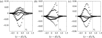
Comparison of normal form-induced stress budgets between cases R1 (empty symbols) and R2 (filled symbols): (a) streamwise, (b) wall-normal and (c) spanwise components. Lines: shear production (- - - - R1, —— R2). Symbols: ▿, pressure work; ▵,
 $-P_{w}$
; ○, viscous dissipation and diffusion. All terms normalized by
 $u_{{\it\tau}}^{4}/{\it\nu}$
.

Figure 7 shows the dispersive stress budgets. Two significant sources are present: the shear production and the pressure work. The shear production is due to the work of the mean flow against the form-induced stress; it contributes to
 $\langle \widetilde{u}^{2}\rangle$
only. The pressure work of WKE can be written as
 $$\begin{eqnarray}\left\langle \widetilde{u}_{i}\frac{\partial \widetilde{P}}{\partial x_{i}}\right\rangle _{s}=-\frac{\partial \langle \widetilde{P}\widetilde{v}\rangle _{s}}{\partial y}+\langle \overline{u}\rangle _{s}\left\langle \frac{\partial \widetilde{P}}{\partial x}\right\rangle ,\end{eqnarray}$$
with the two terms on the right-hand side being the pressure transport and the energy gained from the mean flow working against the form drag; the latter is shown as contributing significantly to
 $\langle \widetilde{u}^{2}\rangle$
and is the only source of
 $\langle \widetilde{v}^{2}\rangle$
and
 $\langle \widetilde{w}^{2}\rangle$
. The WKE is partly converted to TKE through wake production, and partly dissipated into heat. As the roughness height increases from R1 to R2, a larger portion of
 $\langle \widetilde{v}^{2}\rangle$
and
 $\langle \widetilde{w}^{2}\rangle$
is converted to Reynolds stresses instead of being directly dissipated, due to further separation between the roughness length scale and the viscous length scale.
4. Conclusions
DNS are carried out in open-channel flows over sandgrain roughness in the transitionally and the fully rough regimes. A DA technique is applied to separate the spatial disturbance of the time-averaged field and the turbulent field. Significant spatial variations of time-averaged flow quantities are generated due to the three-dimensionality of the roughness geometry. The form-induced stresses are small compared to their Reynolds stress counterparts, but the magnitude of this difference becomes smaller as the roughness height increases.
The work of the form drag near
 $k_{c}$
converts mean-flow energy to wake energy, which is partly dissipated into heat and partly converted to turbulence through wake production. The intensified wall-normal turbulent fluctuations lead to higher pressure work near
 $k_{c}$
, and more homogeneous energy redistribution between the Reynolds stresses. In the fully rough regime, the wake dynamically affects the region of
 $\langle \overline{v^{\prime 2}}\rangle$
generation, while in the transitionally rough regime, its effect is limited below
 $k_{c}$
.
Despite significant transfer from the wake to the turbulent component in the wall-normal and spanwise directions, for the streamwise component the conversion is mostly from turbulence to wake energy, further contributing to a more even TKE redistribution; this is possibly due to the larger turbulent scales that are associated with this Reynolds stress component. The wake production of TKE, however, is negligible, because its values for the three normal Reynolds stresses tend to cancel out, and the magnitudes of total TKE production and dissipation are greater than the energy redistributed.
The present results shed some light on the role of the spatial inhomogeneity on the generation of drag in rough-wall boundary layers. The spatial inhomogeneity, being dependent on the roughness geometry, and in turn altering the energy redistribution and strongly affecting the Reynolds shear stress through its production, may provide the link between geometry detail and the dynamics in the roughness sublayer. Furthermore, the fact that the wake energy depends on the work of mean flow against the form drag as a source term suggests that the wake field is more persistent compared to turbulence in a non-equilibrium boundary layer: while the turbulence production relies on active fluctuations and the mean shear, the presence of the wake requires non-zero mean velocity only. The persistent wake indicates strong interactions between the roughness sublayer and the outer layer, insensitive to the variation of the outer-layer conditions.
Acknowledgements
Support from Hydro Québec, the Natural Science and Engineering Research Council of Canada (NSERC), and the High Performance Computing Virtual Laboratory (HPCVL) is acknowledged.