


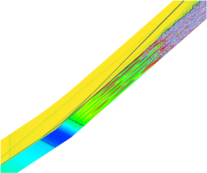


1. Introduction
Laminar–turbulent transition in supersonic and hypersonic boundary layers has been studied for several decades, owing to its importance to the development of high-speed vehicles. However, the boundary layer in external or internal flows of a vehicle may frequently encounter shock waves generated by an adjacent or opposite surface (Gaitonde Reference Gaitonde2015). This shock–boundary layer interaction (SBLI) can significantly alter the transition process in the flow, especially when the adverse pressure gradient induced by shock causes flow separation.
In a typical SBLI, such as a compression-ramp flow, instabilities that trigger transition to turbulence can be classified into two groups. The first type originates from the self-excited, intrinsic instability that is supported by the recirculation flow in the separated region. Since the linear behaviour of the self-excited instability can be described by global stability analysis (GSA) (Theofilis Reference Theofilis2011), it is also called global instability. In addition to the intrinsic dynamics, a SBLI can also behave as a noise amplifier, and the response to extrinsic disturbances (forcing) may be associated with several convective instabilities. In many wind tunnel experiments, both global instability and convective instability are at play. Thus, a comprehensive understanding of instabilities in SBLI is of great importance to transition prediction and flow control.
The dynamics of global instability has been studied intensively in recent years. When the recirculation of the separated flow is strong enough, onset of three-dimensionality can be observed in several SBLI configurations. Examples are shock impingement on a flat plate boundary layer (Robinet Reference Robinet2007; Hildebrand et al. Reference Hildebrand, Dwivedi, Nichols, Jovanović and Candler2018), double-wedge flow (Sidharth et al. Reference Sidharth, Dwivedi, Candler and Nichols2018), double-cone flow (Hao et al. Reference Hao, Fan, Cao and Wen2022), compression-ramp flow (Hao et al. Reference Hao, Cao, Wen and Olivier2021), hollow-cylinder–flare flow (Li & Hao Reference Li and Hao2023). After nonlinear saturation, the self-excited instability usually induces low-frequency streamwise streaks in the vicinity of reattachment (Cao et al. Reference Cao, Hao, Klioutchnikov, Olivier and Wen2021b), which then break down to turbulence farther downstream (Cao et al. Reference Cao, Hao, Klioutchnikov, Wen, Olivier and Heufer2022).
On the other hand, the convective instability is much more complicated than the global instability. Firstly, disturbances in the incoming flow may evolve into first (Mack) mode, second (Mack) mode, streamwise streaks, etc. in the boundary layers ahead of a SBLI. Secondly, multiple amplification mechanisms are possible in the interaction region, such as Görtler instability (Hao et al. Reference Hao, Cao, Guo and Wen2023), nonlinear effects (Lugrin et al. Reference Lugrin, Beneddine, Leclercq, Garnier and Bur2021b; Dwivedi, Sidharth & Jovanović Reference Dwivedi, Sidharth and Jovanović2022) and baroclinic effects (Dwivedi et al. Reference Dwivedi, Sidharth, Nichols, Candler and Jovanović2019). Additionally, the disturbance environment (e.g. its nature, frequency and wavenumber) may have a significant influence on the transition scenarios ‘selected’ by the flow.
Recently, numerous studies focused on Mach 6 flows over a cone–cylinder–flare geometry, where both second mode and shear-layer instability contribute to the transition process (Benitez et al. Reference Benitez, Borg, Paredes, Schneider and Jewell2023a,Reference Benitez, Borg, Scholten, Paredes, McDaniel and Jewellb; Caillaud et al. Reference Caillaud2024), and Mach 5 flows over a hollow-cylinder–flare geometry, for which oblique modes (first mode in nature) play a dominant role and their nonlinear interaction leads to streamwise streaks (Lugrin et al. Reference Lugrin, Beneddine, Garnier and Bur2021a,Reference Lugrin, Beneddine, Leclercq, Garnier and Burb; Threadgill et al. Reference Threadgill, Hader, Singh, Tsakagiannis, Fasel, Little, Lugrin, Bur, Chiapparino and Stemmer2024). Furthermore, the response of compression-ramp flows at Mach 7.7 (Cao et al. Reference Cao, Hao, Guo, Wen and Klioutchnikov2023; Hao et al. Reference Hao, Cao, Guo and Wen2023) and Mach 8 (Dwivedi et al. Reference Dwivedi, Sidharth, Nichols, Candler and Jovanović2019) to upstream forcing were studied using resolvent analysis (also called input–output analysis). It was shown that low-frequency (including steady) streamwise streaks are the dominant modes, though the second mode are important in certain circumstances. It can be concluded from the above studies that, as a noise amplifier, the shock-induced separated flow not only supports the growth of first and second modes, but also promotes the occurrence of streamwise streaks via several mechanisms.
In spite of the rich discussions on global and convective instabilities, complete laminar–turbulent transition data are still lacking. In fact, transition to turbulence in SBLI has been observed in some experiments (Simeonides & Haase Reference Simeonides and Haase1995; Chuvakhov & Radchenko Reference Chuvakhov and Radchenko2020; Lugrin et al. Reference Lugrin, Nicolas, Severac, Tobeli, Beneddine, Garnier, Esquieu and Bur2022; Benitez et al. Reference Benitez, Caillaud, Mcdaniel, Lugrin, Borg, Jewell, Scholten, Paredes, Li and Choudhari2024). But multiple instabilities may coexist in one experiment, making it difficult to identify the dominant mechanism or the interaction between different instabilities. On the other hand, the transition onset may differ significantly between facilities, especially those with different disturbance levels. In a noisy wind tunnel, transition can occur near a reattachment region or even inside the separation bubble (Simeonides & Haase Reference Simeonides and Haase1995; Benay et al. Reference Benay, Chanetz, Mangin, Vandomme and Perraud2006; Sandham et al. Reference Sandham, Schülein, Wagner, Willems and Steelant2014; Currao et al. Reference Currao, Choudhury, Gai, Neely and Buttsworth2020; Davami et al. Reference Davami, Juliano, Scholten and Paredes2023). This flow is usually referred to as transitional SBLI. In a wind tunnel producing low disturbances, however, the experimental flow is more likely to be laminar, and transition is found downstream of reattachment (Benitez et al. Reference Benitez, Borg, Scholten, Paredes, McDaniel and Jewell2023b). Although quiet wind tunnels may produce low-level disturbances, experiments performed in these tunnels are relatively rare. However, high-fidelity numerical simulations and comprehensive stability analyses may shed more light on transition mechanisms in SBLIs, especially for low-disturbance flows (Cao et al. Reference Cao, Hao, Klioutchnikov, Wen, Olivier and Heufer2022; Paredes et al. Reference Paredes, Scholten, Choudhari, Li, Benitez and Jewell2022; Caillaud et al. Reference Caillaud2024). In this way, the main motivation of the present work is to make contribution to understanding transition scenarios in a low-disturbance flow that may occur in quiet tunnels or flight.
This paper addresses the influence of disturbance amplitude on the transition scenarios in a hypersonic compression-ramp flow with laminar separation. Several stability analysis tools are used to identify instability mechanisms that may trigger transition to turbulence in the considered flow. Direct numerical simulation (DNS) is then employed to show that not only the transition onset, but also the transition mechanism is sensitive to the disturbance amplitude. The considered disturbances are weak enough to ensure that the transition to turbulence takes place downstream of reattachment. It will be demonstrated that for a moderate disturbance amplitude, the transition to turbulence is dominated by low-frequency streamwise streaks. When the amplitude is reduced by a factor of four, the high-frequency second mode experiences large growth and predominates the transition process.
2. Stability analysis of the base flow
2.1. Two-dimensional base flow
The flow conditions considered in the present paper are the same as our previous work (Cao et al. Reference Cao, Hao, Klioutchnikov, Wen, Olivier and Heufer2022). The free stream Mach number ( $M_\infty$), Reynolds number (
 $Re_{\infty }$) and temperature (
 $T_{\infty }$) are 7.7,
 $8.6\times 10^6$ m
 $^{-1}$ and 125 K, respectively. To study the transition scenarios in a globally stable flow, a smaller ramp angle 10
 $^{\circ }$, instead of 15
 $^{\circ }$ in Cao et al. (Reference Cao, Hao, Klioutchnikov, Wen, Olivier and Heufer2022), is used here. The length of flat plate and ramp are
 $L = 100$ mm and
 $L_r = 180$ mm, respectively.
For the DNS, the Navier–Stokes equations for unsteady, compressible flow are solved using a finite-difference method that achieves high-order accuracy in space and time. A fifth-order WENO (weighted essentially non-oscillatory) scheme, a sixth-order central-difference scheme and a third-order Runge–Kutta scheme are used for the discretisation of inviscid fluxes, viscous fluxes and time derivatives, respectively. Details about the numerical schemes may be found in Cao (Reference Cao2021). The DNS solver has been validated and used in our previous studies (Cao, Klioutchnikov & Olivier Reference Cao, Klioutchnikov and Olivier2020; Cao et al. Reference Cao, Hao, Klioutchnikov, Olivier, Heufer and Wen2021a,Reference Cao, Hao, Klioutchnikov, Olivier and Wenb, Reference Cao, Hao, Klioutchnikov, Wen, Olivier and Heufer2022).
In the simulation of two-dimensional (2-D) base flow, the number of grid points in the streamwise ( $x$) and wall-normal (
 $y$) directions is 3360 and 320, respectively. In the
 $y$ direction, the mesh is clustered near the wall, and the minimum mesh spacing is
 $\Delta y_w = 4\times 10^{-6}$ m. Free stream parameters are imposed at the inflow and upper boundaries. An isothermal condition is specified at the no-slip wall, and the wall temperature is set at 293 K. A grid-independence study showed a converged solution for the base flow (see the Appendix).
Figure 1 shows the Mach number contour and density gradient contour ( $\boldsymbol {\nabla } (\rho /\rho _\infty ) = \boldsymbol {\nabla }\bar {\rho } = \sqrt {(\partial \bar {\rho }/\partial \bar {x})^2 + (\partial \bar {\rho }/\partial \bar {y})^2}$) of the base flow. Because of the small ramp angle, the shock-induced pressure rise only leads to a small separation bubble around the corner. No secondary separation is found in the separation bubble. The separation and reattachment points are located at
 $x/L = 0.84$ and
 $x/L = 1.14$, respectively. In the following, several stability analysis tools are utilised to study the stability of flow inside the separation bubble, near the reattachment region and downstream of reattachment.
(a) Mach number contour and (b) density gradient contour of the 2-D base flow.

2.2. Global stability analysis
The first step is to show that the base flow supports no self-excited instability (global instability). To this end, GSA is employed to study the temporal stability of the 2-D base flow with respect to three-dimensional (3-D) small-amplitude perturbations. The linearised Navier–Stokes equations can be written in the following operator form:
 \begin{equation} \frac{\partial \boldsymbol{U}'}{\partial t} = \boldsymbol{\mathcal{A}} \boldsymbol{U}', \end{equation}
where  $\boldsymbol {U}'$ includes the perturbation variables and
 $\mathcal {A}$ is the linearised Navier–Stokes operator. The perturbation
 $\boldsymbol {U}'$ is assumed to be in the form
 \begin{equation} \boldsymbol{U}'(x,y,z,t) = \hat{\boldsymbol{U}}(x,y) \exp \left[ {\rm i}\frac{2{\rm \pi}}{\lambda}z - {\rm i}(\omega_r + {\rm i}\omega_i)t \right], \end{equation}
where  $\hat {\boldsymbol {U}}$ is the 2-D eigenfunction,
 $\lambda$ denotes the spanwise wavelength,
 $\omega _r$ is the angular frequency and
 $\omega _i$ is the temporal growth rate. The resulting eigenvalue problem is solved using an in-house GSA solver as described in Hao et al. (Reference Hao, Cao, Wen and Olivier2021). To reduce the memory requirement of the GSA and the following resolvent analysis, we restrict the computational domain to
 $x/L = 0.4$–
 $2.5$.
In addition to the 10 $^{\circ }$ ramp angle case, a base flow for 11
 $^{\circ }$ ramp angle is also considered to clarify the global stability boundary. Figure 2 provides the growth rates of the least stable mode as a function of
 $\lambda$ for the 10
 $^{\circ }$ and 11
 $^{\circ }$ cases. It is seen that the 11
 $^{\circ }$ case is marginally stable with the peaking growth rate being slightly smaller than zero. The spanwise wavelength for the mode with largest growth rate is
 $\lambda /L = 0.140$. In contrast, the 10
 $^{\circ }$ case is much more stable, and the growth rate peaks at
 $\lambda /L = 0.105$. The eigenvalue spectrum for the least stable mode at
 $\lambda /L = 0.105$ is shown in the Appendix, together with a grid-independence study for the GSA. It is noted that the behaviour of the least stable mode, that is, the dominant mode shifts to a longer wavelength and a short-wavelength mode occurs as the ramp angle is increased, is consistent with the results of Hao et al. (Reference Hao, Cao, Wen and Olivier2021). The above GSA results justify the choice of base flow as the aim of this paper is to study convective instability, rather than global instability. In the following, we investigate the response of base flow (10
 $^{\circ }$ case) to upstream forcing.
The GSA results for 10 $^{\circ }$ and 11
 $^{\circ }$ cases: growth rates of the least stable mode as a function of spanwise wavelength.

2.3. Resolvent analysis
Here, resolvent analysis is employed to identify the response of the globally stable base flow to external small-amplitude disturbances  $\boldsymbol {d}'$ that are periodic in time and in the spanwise direction. Hence, a forcing term is added to (2.1) as
 \begin{equation} \frac{\partial \boldsymbol{U}'}{\partial t} = \boldsymbol{\mathcal{A}} \boldsymbol{U}' + \boldsymbol{\mathcal{B}} \boldsymbol{d}', \end{equation}
where operator  $\boldsymbol {\mathcal {B}}$ constrains the forcing to a specific location. To be consistent with the following DNS, the forcing is added on a wall-normal plane at
 $x/L = 0.5$. Here
 $\boldsymbol {d}'$ is given by
 \begin{equation} \boldsymbol{d}'(x,y,z,t) = \hat{\boldsymbol{d}}(x,y) \exp \left( {\rm i}\frac{2{\rm \pi}}{\lambda}z - {\rm i} \omega_r t \right). \end{equation}
As a globally stable flow is considered, the long-time solution of (2.3) takes the same form
 \begin{equation} \boldsymbol{U}'(x,y,z,t) = \hat{\boldsymbol{U}}(x,y) \exp \left( {\rm i}\frac{2{\rm \pi}}{\lambda}z - {\rm i} \omega_r t \right). \end{equation}
Substituting (2.4) and (2.5) into (2.3) gives
 \begin{equation} \hat{\boldsymbol{U}} = \boldsymbol{RB}\hat{\boldsymbol{d}}, \boldsymbol{R} = (-{\rm i}\omega_r \boldsymbol{I} - \boldsymbol{A})^{{-}1}, \end{equation}
where  $\boldsymbol {R}$ is the resolvent matrix and
 $\boldsymbol {I}$ is the identity matrix.
In the present analysis, we aim to find the forcing and response pair that maximises the energy amplification. The maximum amplification is referred to as optimal gain and defined by
 \begin{equation} \sigma^2(\lambda,\omega_r) = \max_{\hat{\boldsymbol{d}}} \frac{\|\hat{\boldsymbol{U}}\|_E}{\|\boldsymbol{B}\hat{\boldsymbol{d}}\|_E}, \end{equation}
where the energy norm is evaluated according to Chu energy (Chu Reference Chu1965). The optimisation problem (2.7) is then converted to an eigenvalue problem and solved using an in-house code. Details about the numerical treatment can be found in Hao et al. (Reference Hao, Cao, Guo and Wen2023).
According to previous studies on the compression-ramp flow (Dwivedi et al. Reference Dwivedi, Sidharth, Nichols, Candler and Jovanović2019; Cao et al. Reference Cao, Hao, Guo, Wen and Klioutchnikov2023; Hao et al. Reference Hao, Cao, Guo and Wen2023), the optimal response of hypersonic flow over a compression ramp is low-frequency (including steady) streamwise streaks with a specific spanwise wavelength. Therefore, we first perform resolvent analysis to find the most amplified streaks. The optimal gain as a function of spanwise wavelength for steady streaks is shown in figure 3(a). It is clear that the maximum optimal gain is achieved at  $\lambda /L = 0.018$. Subsequently, we consider the frequency response of base flow to the streamwise streaks with a wavelength of
 $\lambda /L = 0.018$. As shown in figure 3(b), the optimal gain remains constant at low frequencies and drops quickly when
 $\omega _r L/U_{\infty } > 1$. This low-pass feature is consistent with other studies for SBLI (Dwivedi et al. Reference Dwivedi, Sidharth, Nichols, Candler and Jovanović2019; Bugeat et al. Reference Bugeat, Robinet, Chassaing and Sagaut2022). It has been proved by Hao et al. (Reference Hao, Cao, Guo and Wen2023) and Cao et al. (Reference Cao, Hao, Guo, Wen and Klioutchnikov2023) that the main amplification mechanism of streamwise streaks is Görtler instability that is supported by the streamline curvature near separation and reattachment positions. In other words, streamwise streaks can experience large amplification in the SBLI region.
(a) Optimal gain as a function of spanwise wavelength for the steady streaks. (b) Optimal gain as a function of angular frequency at  $\lambda / L = 0.018$.

2.4. Local stability analysis
In the considered compression-ramp flow, SBLI only takes place near the corner. For the downstream flow over the ramp, its behaviour resembles a flat-plate boundary layer. Hence, typical convective instabilities such as Mack's first/second mode may be present here.
Lastly, we use linear stability theory (LST) to identify local convective instability in the reattached boundary layer on the ramp. The considered small-amplitude disturbance is in the following form:
 \begin{equation} \boldsymbol{\phi} ' (x,y,z,t) = \boldsymbol{\varphi}(y)\exp({\text{i}(\alpha x + \beta z - \omega t)}), \end{equation}
where  $\boldsymbol {\varphi } = (\hat \rho,\hat u,\hat v,\hat w,\hat T)^{\rm {T}}$ is the eigenfunction,
 $\alpha = \alpha _r + \text {i} \alpha _i$,
 $\beta$ and
 $\omega$ denote the spanwise wavenumber and the angular frequency, respectively. Here
 ${\alpha }_r$ is the streamwise wavenumber, and
 $-{\alpha }_i$ is the spatial growth rate. The numerical details of the LST code may be found in Cao et al. (Reference Cao, Hao, Guo, Wen and Klioutchnikov2023) and Guo, Hao & Wen (Reference Guo, Hao and Wen2023). Three boundary layer profiles at
 $x/L$ = 1.4, 1.8 and 2.5 are used as the base flow for LST analysis. To find the most unstable second mode, the spanwise wavenumber
 $\beta$ is set to zero. The resulting spatial growth rate as a function of frequency is shown in figure 4. As expected, the most significant frequency drops quickly as the boundary layer evolves in the streamwise direction. The growth rate peaks at 775, 660 and 525 kHz for
 $x/L$ = 1.4, 1.8 and 2.5, respectively. These values are used to compare with the DNS data later. In addition, LST analysis is carried out for non-zero spanwise wavenumber, and no unstable first mode is found for the boundary layer over the ramp. Necessary LST analysis is also performed below to facilitate the understanding of instabilities associated with the transition process.
Spatial growth rates as a function of frequency for the most unstable second mode at different streamwise locations.

3. Transition to turbulence in the presence of random disturbances
On the basis of previous stability analysis results, we then explore transition scenarios in the compression-ramp flow using DNS. As the main destabilising mechanisms are low-frequency streamwise streaks and high-frequency second mode, it is conjectured that their contribution to transition lies in different regions, that is, near reattachment and far downstream of reattachment. To this end, external disturbances with different amplitudes are introduced in DNS to investigate the transition process associated with different instabilities.
According to the resolvent analysis, the spanwise wavelength of the most amplified streaks is  $\lambda /L = 0.018$ (
 $\lambda = 1.8$ mm). Hence, the width of compression ramp is set as 14.4 mm, which allows the DNS to capture eight streaks. Accordingly, 220 grid points are equispaced in the spanwise (
 $z$) direction. To study the ‘natural’ transition process that may occur in wind tunnel experiments or during flights, random disturbances are introduced in the incoming laminar flow. Similar to Hader & Fasel (Reference Hader and Fasel2018) and Cao et al. (Reference Cao, Hao, Guo, Wen and Klioutchnikov2023), the random forcing takes the following form:
 \begin{equation} w^{\prime}_{j,k}/U_\infty = A_{noise}(2r-1), \end{equation}
where the  $j$ and
 $k$ refer to the grid point indices in the
 $y$ and
 $z$ directions,
 $A_{noise}$ denotes the amplitude of perturbations and
 $r$ is a pseudorandom number (ranging from 0 to 1) generated by the rand() function in C. Specifically, random spanwise velocity perturbations (
 $w^\prime /U_\infty$) are superimposed on the
 $y$–
 $z$ plane at
 $x/L = 0.5$ (i.e. for
 $1 \leqslant j \leqslant 320$ and
 $1 \leqslant k \leqslant 220$). Three noise levels are considered in this paper,
 $A_{noise} = 6\,\%$, 3 % and 1.5 %. For convenience, the three cases are labelled as A6, A3 and A1.5. To ensure a sufficient time for the convection of disturbances through grid points, the perturbation is updated every 50 time steps. Because the time step size for these cases is set to
 $4 \times 10^{-9}$ s to ensure a stable computation, the time interval for updating the spanwise velocity becomes
 $\Delta t = 2 \times 10^{-7}$ s (or
 $\Delta tU_\infty /L = 0.0035$). Accordingly, the sampling frequency for collecting data is 4.93 MHz. As shown by Hader & Fasel (Reference Hader and Fasel2018) and Cao et al. (Reference Cao, Hao, Guo, Wen and Klioutchnikov2023), the induced disturbances have a broadband spectrum in both frequency and wavelength, which allows the flow to ‘naturally’ select preferred modes.
After the flow is fully developed, transition to turbulence is observed for all three cases. It should be mentioned that, to capture a complete transition process for case A1.5, the ramp length and the number of streamwise grid points are increased to 250 mm and 3920, respectively. Figure 5 shows the streamwise distributions of Stanton number for the three cases, which is defined as
 \begin{equation} St = \frac{q_w}{\rho_\infty U_\infty c_p (T_{aw} - T_w)}. \end{equation}
Here,  $q_w$ denotes the surface heat flux,
 $c_p$ is the specific heat capacity and
 $T_{aw}$ is the adiabatic wall temperature. The solid lines correspond to spanwise-averaged values, whereas the dashed lines represent the time- and spanwise-averaged
 $St$. As shown in figure 5, the length of separated region is not affected by the considered disturbance amplitudes, and the flow upstream and inside the separation bubble remains laminar for all cases. However, transition to turbulence occurs downstream of reattachment. As expected, the transition onset moves downstream with decreasing disturbance amplitude. Interestingly, the transition length for case A1.5 is much larger than cases A6 and A3, which may indicate a different transition scenario for case A1.5. It can be estimated that the Stanton number in the turbulent region rises by a factor of four in comparison with the undisturbed laminar flow.
Streamwise distribution of Stanton number for cases A6, A3 and A1.5. Solid lines represent the spanwise-averaged  $St$ for an instantaneous flow. Blue dashed lines correspond to time- and spanwise-averaged values.

Figure 6 provides an instantaneous flow field for case A6 showing the complete laminar–turbulent transition process. The introduced disturbances decay rapidly on the flat plate but experience large amplification in the vicinity of separated region (Cao et al. Reference Cao, Hao, Guo, Wen and Klioutchnikov2023). Downstream of reattachment, distinct streamwise heat-flux streaks can be observed, which are the footprint of spanwise-modulated boundary layers (i.e. boundary-layer streaks). It can be estimated that the spanwise wavelength of the streaks is approximately 1.8 mm, which agrees well with the resolvent analysis. Note that the streaks are unsteady and exhibit a low-frequency feature, as shown below. Farther downstream, the streaks break down to turbulence quickly.
Instantaneous flow for case A6. Stanton number is shown on the surface, together with isolines of zero skin friction coefficient. Density gradient at  $z/L = 0$ is shown to indicate the SBLI. The
 $Q$-criteria is used to visualise the transitional and turbulent flow.

Figure 7 presents the temporal history and the corresponding power spectra density (PSD) of the Stanton number and surface pressure at  $(x/L, z/L) = (1.4, 0.072)$, which is slightly upstream of transition onset (
 $x/L \approx 1.5$). The Stanton number signal mainly exhibits a low-frequency feature with the most energetic components being less than 40 kHz. Although a local peak can be found around 700 kHz, it is very weak compared with the low-frequency parts. The low-frequency characteristic is consistent with the resolvent analysis and our previous studies (Cao et al. Reference Cao, Hao, Guo, Wen and Klioutchnikov2023). It should be mentioned that although the spanwise- or time-averaged
 $St$ is approximately
 $2 \times 10^{-3}$ (see figure 5), the instantaneous
 $St$ can reach as high as
 $5 \times 10^{-3}$. In fact, the relative standard deviation for the Stanton number signal in figure 7(a) is 77 %. For the pressure signal, the peaking frequency is close to the frequency of the most unstable second mode (775 kHz) revealed by LST. But the high-frequency part is not significant in comparison with cases A3 and A1.5 (see below). Figure 8 shows the PSD contour for Stanton number and pressure signals along the centreline of wall. It is seen that upstream of transition onset, the Stanton number signal is dominated by low-frequency components, and no evident peak is found for the pressure signal. Therefore, it can be concluded that the transition to turbulence in case A6 is dominated by low-frequency streamwise streaks. As this transition scenario corresponds to a relatively high-amplitude forcing (but not as high as transitional SBLI), the streak-induced transition observed in some experiments (e.g. Chuvakhov et al. Reference Chuvakhov, Borovoy, Egorov, Radchenko, Olivier and Roghelia2017; Chuvakhov & Radchenko Reference Chuvakhov and Radchenko2020) has close similarity to case A6.
(a,b) Temporal history of Stanton number and surface pressure at  $(x/L, z/L) = (1.4, 0.072)$ for case A6. (c,d) The PSD of the signal shown in panels (a,b).

Contour of  $\log (PSD)$ for (a) Stanton number and (b) surface pressure signals along the centreline of wall for case A6.

For case A3, the transition onset moves downstream to  $x/L \approx 1.9$. As illustrated in figure 9, due to a smaller disturbance amplitude, the streamwise heat-flux streaks are weaker than case A6. In addition, the reattachment line is less distorted. On the other hand, the spanwise wavelength of streaks is still 1.8 mm.
Instantaneous flow for case A3. Stanton number is shown together with isolines of zero skin friction coefficient. Density gradient at  $z/L = 0$ is shown to indicate the SBLI. The
 $Q$-criteria is used to visualise the transitional and turbulent flow.

The temporal history and corresponding PSD of Stanton number and surface pressure at ( $x/L, z/L$) = (1.8, 0.072) for case A3 are shown in figure 10. For the Stanton number signal, although low-frequency components are still dominant, a noticeable local peak can be observed around 760 kHz (see figure 10c). However, the surface pressure signal is dominated by high frequencies, which also peaks at 760 kHz. This is reasonable as the boundary-layer streaks have an insignificant influence on the surface pressure. Additionally, higher harmonics of the peaking frequency can be found in figure 10(d). These facts are typical of the second-mode instability of the boundary layer on the ramp. The reason for the discrepancy in the peaking frequency obtained from DNS and LST may be as follows. In the DNS, the occurrence of streamwise streaks modifies the profile of boundary layer. For instance, the boundary layer thickness is modulated in the spanwise direction. As a result, the second modes evolving in the distorted boundary layer are different from those in a spanwise homogeneous base flow. Nevertheless, it can be concluded that both low-frequency streamwise streaks and second-mode instability waves exist in the transitional flow for case A3. Figure 11 provides the PSD contour for Stanton number and pressure signals along the centreline of wall. It can be observed that low-frequency streamwise streaks grow rapidly downstream of reattachment and remain strong until transition onset (
 $x/L = 1.9$). For the second mode, however, it is remarkable only downstream of
 $x/L = 1.7$, as seen in figure 11(b). To fully understand the breakdown mechanism in case A3, a thorough examination of the interaction between second mode and streamwise streaks may be necessary (Chen, Zhu & Lee Reference Chen, Zhu and Lee2017; Paredes, Choudhari & Li Reference Paredes, Choudhari and Li2019).
(a,b) Temporal history of Stanton number and surface pressure at  $(x/L, z/L) = (1.8, 0.072)$ for case A3. (c,d) The PSD of the signal shown in panels (a,b).

Contour of  $\log (PSD)$ for (a) Stanton number and (b) surface pressure signals along the centreline of wall for case A3.

When the disturbance amplitude is further reduced to 1.5 %, the transition scenario tends to be different. Figure 12 presents an instantaneous flow for case A1.5. Because of the low amplitude, the streamwise streaks become much weaker than cases A6 and A3, and the reattachment line is almost straight. Nevertheless, the spanwise wavelength of streaks remains at 1.8 mm. It is conceivable that the weak streaks may decay and transition may not take place downstream if there are no other modes. However, the second-mode instability waves grow rapidly in the boundary layer at a large distance downstream of reattachment, as shown in the surface heat flux distribution at  $x/L = 2.0$–
 $3.0$. It is noted that the occurrence of second mode is influenced by the streamwise streaks. Consequently, turbulent spots are randomly distributed ahead of the fully turbulent flow.
Instantaneous flow for case A1.5. Stanton number is shown together with isolines of zero skin friction coefficient. Density gradient at  $z/L = 0$ is shown to indicate the SBLI. The
 $Q$-criteria is used to visualise the transitional and turbulent flow.

The Stanton number and surface pressure signals at  $(x/L, z/L) = (2.5, 0.072)$ and the corresponding PSD are given in figure 13. In comparison with cases A6 and A3, though both high-frequency and low-frequency peaks are present in the Stanton number signal, the low-frequency parts have a smaller PSD. It is reasonable due to the smaller disturbance amplitude. Interestingly, the low-frequency part in figure 13(c) matches well with the resolvent analysis. Note that the green curve is taken from figure 3(b) but has been premultiplied. This agreement again verifies the resolvent analysis results. For the surface pressure signal, it peaks at 470 kHz, which is close to the frequency of the most unstable planar second mode at
 $x/L = 2.5$ (525 kHz). It is noted that the intermittently occurring high-frequency packets (figure 13b) are a result of the low-frequency boundary-layer streaks.
(a,b) Temporal history of Stanton number and surface pressure at  $(x/L, z/L) = (2.5, 0.072)$ for case A1.5. (c,d) The PSD of the signal shown in panels (a,b). The green line corresponds to the curve shown in figure 3(b) with a different magnitude.

Figure 14 illustrates the PSD contour for Stanton number and pressure signals along the centreline of wall. For the Stanton number, its low-frequency components virtually remain neutral until transition onset ( $x/L \sim 2.6$), whereas its high-frequency part starts growing at
 $x/L \approx 1.5$. This high-frequency component results from the second-mode instability. As shown in the pressure data (figure 14b), the second mode grows rapidly downstream of
 $x/L = 1.5$. To identify the frequency of the most unstable planar second mode along streamwise direction, LST analysis is performed from
 $x/L = 1.5$ to 3.0 using the 2-D base flow. The black line represents the obtained frequencies. It is apparent that the peak frequencies in the DNS data agree well with LST results, especially upstream of
 $x/L = 2.2$. This is because the boundary layer is less distorted by the weak streaks there. The slight discrepancy in the downstream region may be again attributed to the deviation of boundary layer in the 3-D simulation to that in the 2-D base flow. The above findings confirm the dominance of the planar second mode in the boundary layer transition for case A1.5. Owing to a very low-level forcing, this transition scenario is more likely observed in quiet wind tunnels (Benitez et al. Reference Benitez, Borg, Scholten, Paredes, McDaniel and Jewell2023b).
Contour of  $\log (PSD)$ for (a) Stanton number and (b) surface pressure signals along the centreline of wall for case A1.5.

4. Conclusion
In the present paper, the transition to turbulence in a Mach 7.7 compression-ramp flow excited by upstream forcing was studied. A small ramp angle was used to produce a weakly separated flow. Global stability analysis was firstly performed to identify the global instability of two compression-ramp flows and justify the choice of base flow. Then, resolvent analysis was carried out to reveal the response of base flow to upstream forcing. It was shown that the optimal response is low-frequency streamwise streaks with a specific spanwise wavelength. Subsequently, LST was utilised to analyse the local second-mode instability in the boundary layer downstream of reattachment.
A DNS was then performed to explore the transition scenarios associated with the instabilities identified by stability analyses. By introducing random disturbances with different amplitudes upstream of separation, several transition scenarios were revealed. For a large amplitude (case A6), strong streamwise streaks emerge near the reattachment region. The streaks have a spanwise wavelength of 1.8 mm and exhibit a low-frequency response, which are consistent with the resolvent analysis. Transition to turbulence is accomplished via the breakdown of streamwise streaks. When the disturbance amplitude was reduced to 3 % (case A3), the transition onset moves downstream, and high-frequency second mode becomes significant in the surface heat flux and pressure signals. Hence, both low-frequency streamwise streaks and a high-frequency second mode contribute to the transition process for case A3. When the amplitude was further decreased to 1.5 % (case A1.5), the streamwise streaks become much weaker, but the second mode grows rapidly in the downstream region. Although its growth is affected by the low-frequency streamwise streaks, the second mode plays a dominant role in the transition to turbulence for case A1.5. Therefore, it can be concluded that for the considered compression-ramp flow, not only the transition onset, but also the transition mechanism is sensitive to upstream disturbance amplitude.
In our previous work (Cao et al. Reference Cao, Hao, Klioutchnikov, Wen, Olivier and Heufer2022), the ramp angle is larger than the present cases, which causes the flow to be globally unstable. Thus, the transition to turbulence is completely induced by the global instability, and the transition process is independent of initial disturbances and can be accomplished without external forcing. However, this paper demonstrates that for a globally stable flow, the transition scenarios with respect to convective instability are highly dependent on the amplitude of external disturbances. It is reminiscent of recent experimental studies on Mach 6 flows over a cone–cylinder–flare geometry (Benitez et al. Reference Benitez, Borg, Scholten, Paredes, McDaniel and Jewell2023b, Reference Benitez, Caillaud, Mcdaniel, Lugrin, Borg, Jewell, Scholten, Paredes, Li and Choudhari2024), where the transition onset differed in different facilities under the same flow condition or in the same facility with different noise levels. It is finally noted that for the above Mach 6 flow, first mode, second mode and streaks may coexist, whereas only second mode and streaks appear in the present Mach 7.7 cold-wall flow. Nevertheless, both studies showed multiple possible transition paths to turbulence in low-disturbance flows.
Funding
This work was supported by the National Natural Science Foundation of China (no. 12302304).
Declaration of interests
The authors report no conflict of interest.
Appendix. Grid independence
A grid-independence study for the base flow is firstly conducted. Two mesh resolutions are considered, i.e.  $2240\times 240$ and
 $3360\times 320$. Figure 15 provides the streamwise distributions of surface pressure coefficient
 $C_p = (p - p_\infty )/(0.5 \rho _\infty U^2_\infty )$ and Stanton number for the two meshes. It is clear that a converged solution for the base flow is achieved. Nevertheless, the fine mesh is used in the DNS to accurately capture the transition process.
Grid-independence study for the base flow: streamwise distributions of surface pressure coefficient and Stanton number for different mesh resolution: coarse mesh,  $2240\times 240$; fine mesh,
 $3360\times 320$.

To examine grid independence for the GSA, we consider the least stable mode at  $\lambda /L = 0.105$ for the 10
 $^{\circ }$ case (see figure 2). Figure 16 shows the eigenvalue spectra for this mode with two mesh resolutions. The overlap of leading modes verifies the grid independence for the GSA.
Grid-independence study for the GSA: eigenvalue spectra at  $\lambda /L = 0.105$ for different mesh resolution: square, coarse mesh; circle, fine mesh.

Subsequently, grid independence for the resolvent analysis is studied for the streaks at  $\lambda /L = 0.018$. For the fine mesh, the optimal gain at frequencies
 $\omega _r L/U_{\infty } = 0.1, 1$ and 10 is shown in figure 17 together with results for the coarse mesh. The almost identical solution indicates that the coarse mesh is sufficient for resolvent analysis.
Grid-independence study for the resolvent analysis: optimal gain as a function of angular frequency at  $\lambda /L = 0.018$: line, coarse mesh; square, fine mesh.



