1. Introduction and statement of the main results
We consider polynomial differential systems

defined in the plane $ {\mathbb {R}}^2$ . Here, the dot denotes the derivative with respect to the time $t$
 . We are interested in the subclass of these polynomial differential systems having an equilibrium point whose linear part has eigenvalues purely imaginary. After an affine change of variables and a rescaling of the time (if necessary) such polynomial differential systems can be written into the form:

where $P_n$ and $Q_n$
 are polynomials of degree $n$
 , which do not have either constant or linear termsSão.
The problem of distinguishing whether the equilibrium point at the origin of system (1.2) is a centre or a focus is a classical problem, known as the centre–focus problem. Even though this problem was partially solved by Lyapunov (see [Reference Liapunov22]), it has been studied for some fixed values of the degree $n$ for more than a century by many authors. The only family completely investigated is the family of the polynomial differential systems of degree $2$
 , denoted simply by quadratic systems. The study of this family was started by Dulac in 1908 in [Reference Dulac11], and also performed by Kaptyen some years later (see [Reference Kaptyen20, Reference Kaptyen21]). Up to the work of Frommer [Reference Frommer13], the conditions for the existence of a centre in that family were not published. The correct centre conditions were published by Saharnikov [Reference Saharnikov31] and later by Sibirskiĭ [Reference Sibirskiĭ32]. The centre conditions are simpler and the centre–focus problem is easier to solve if the system is written in complex coordinates (see [Reference Zoładek33]). For the complete cubic family (when in systems (1.2) we have $n=3$
 ), the problem remains unsolved.
In 1992, Galeatti and Villarini in [Reference Galeatti and Villarini14] proved that if the degree $n$ of a polynomial differential system (1.2) is even such a system cannot have a global centre. Recently, Llibre and Valls proved the same in an easier way (see [Reference Llibre and Valls25]). In [Reference Conti7], Conti proposed the following problem: To classify all polynomial differential systems of degree odd having global centres, this is a very difficult problem.
It is well known that all the centres of the polynomial differential systems (1.2) with $n=1$ (i.e. of the linear differential systems) are global.
For $n=3$ , the global linear centres (i.e. the centres with purely imaginary eigenvalues) and the global nilpotent centres (i.e. the centres having both eigenvalues zero but its linear part is not identically zero) having only homogeneous nonlinearities of degree $3$
 are completely classified in [Reference García-Saldaña, Llibre and Valls15] and [Reference García-Saldaña, Llibre and Valls16], respectively. Moreover, also for $n=3$
 in [Reference Barreira, Llibre and Valls3] the authors classify the global centres of the Hamiltonian systems that are reversible with respect to the $x$
 -axis, and in [Reference Barreira, Llibre and Valls4] the authors classify the global nilpotent centres of the cubic Hamiltonian systems.
When $n=5$ and for systems (1.2) with homogeneous nonlinearities of degree $5,$
 in [Reference Llibre and Valls26] the authors classify their global linear centres for the subclass of such systems that are reversible with respect to the $x$
 -axis, and in [Reference García-Saldaña, Llibre and Valls17] with respect to the $y$
 -axis.
A natural continuation in the classification of the global centres is to consider another family of polynomial differential systems (1.2) with $n=5$ . Thus, in this paper we consider the following class of quintic polynomials differential systems

in the plane $ {\mathbb {R}}^2$ . Then, the main result of this paper is as follows.
Theorem 1.1 The polynomial differential systems (1.3) have a global centre at the origin of coordinates if, and only if, the following conditions hold: $a_{32}\leq 0,\, a_{50}\leq 0 \text { and, } a_{14}=a_{41}=a_{23}=a_{05}=0.$
Before starting with the classification of the global centre it is necessary to solve the centre–focus problem. The classification of the centres has been possible despite six parameters are appearing. Thus, in the following result we provide the answer to the centre–focus classification problem.
Theorem 1.2 The polynomial differential systems (1.3) have a centre at the origin of coordinates and the origin is the unique equilibrium point of the system if, and only if, the following conditions hold: $a_{50}\leq 0 \text { and }a_{41}=a_{23}=a_{05}=0.$
This paper is structured as follows. In § 2 we provide the necessary definitions, results, and an algorithm to obtain the coefficients of the return map, the so-called Lyapunov constants. In § 3 and 4 we prove theorems 1.2 and 1.1, respectively.
2. Preliminaries
In this section, we recall some classical concepts which are necessary to state and prove the results of this paper.
In § 2.1, we recall how to obtain the coefficients of the return map (i.e. the Lyapunov constants) near a monodromic equilibrium point (i.e. a focus or a centre). In § 2.2, we define the Bautin ideal and the centre variety. In § 2.3, we recall the Poincaré compactification.
Finally, in § 2.4, we recall the result for classifying the global centres.
2.1. The centre conditions
We consider a polynomial differential system of degree $n$ with an equilibrium point at the origin of coordinates having its Jacobian matrix purely imaginary eigenvalues, i.e. we consider a system (1.2). So, the origin is a focus or a centre.
A non-constant analytical function defined in a neighbourhood $\Omega$ of the origin, $H:\Omega \subset \mathbb {R}^2\rightarrow \mathbb {R}^2,$
 is a first integral of system (1.2) if it is constant along any solution $\gamma$
 or, equivalently,

In order to distinguish whether the origin is a centre we shall use the Poincaré–Lyapunov theorem (see [Reference Ilyashenko and Yakovenko19, Reference Liapunov23, Reference Poincaré28, Reference Romanovski and Shafer29]):
Theorem 2.1 The polynomial differential system (1.2) has a centre at the origin if and only if it admits a local analytic first integral of the form:

In addition, the existence of a formal first integral $H$ of the above form implies the existence of a local analytic first integral.
The necessary conditions for the existence of a first integral (2.2) for system (1.2) are obtained by looking for a formal series (2.2) satisfying (2.1). Although (2.1) is not always satisfied, it is always possible to choose coefficients of the formal power series (2.2) that satisfy the following equation:

(see [Reference Blows and Lloyd5, Reference Liapunov24]). We remark that any non-zero $L_j$ obstructs the origin to be a centre. Then, when at least one $L_j$
 is different from zero, it is a Lyapunov constant in a neighbourhood of the origin. Hence, system (1.2) has no local analytic first integral and we say that the equilibrium point is a weak focus of order $k$
 if the first non-zero coefficient in (2.3) is $L_k.$
 The coefficient $L_j$
 in (2.3) is called the $j$
 -th Lyapunov constant. The stability of the origin is given by the sign of the first non-zero $L_j.$
 Moreover, note that the constants $L_j$
 are rational functions whose numerators are polynomials depending on the coefficients of the polynomial system (1.2).
In order to compute the first $N$ Lyapunov constants, we need to compute the terms up to order $2N+2$
 in the series (2.2), i.e.:

Then, for each $i=3,\,\ldots,\,2N+2,$ we equate to zero the coefficients of terms of degree $i$
 in the expression:

Hence, starting with $i=3$ we solve in a recurrent way each linear system of $i+1$
 equations with $i+1$
 variables, $q_{p-\ell,\ell }$
 for $\ell =0,\,\dots,\,p$
 . All linear systems corresponding to odd degrees, $i=2j+1,$
 have a unique solution in terms of the previous values of $q_{p-\ell,\ell }$
 . As the determinant of the linear system that corresponds to an even degree, $i=2j+2,$
 vanishes, we need to add an extra condition so that the linear system has a unique solution. In fact, in this step, we have one equation more than the number of variables. We add suitable equations, for the terms $(x^{2}+y^{2})^{j+2}$
 for example, so that the derivative over the associated vector field becomes:

Therefore, we define the Lyapunov constants associated with the extra conditions given above. In this context, it is well-known that the first non-vanishing coefficient of (2.5) has an odd subindex, and $L_{2k+1}$ is called the $k$
 th-order Lyapunov constant of system (1.2). An interesting property, described in [Reference Roussarie30] and proved in [Reference Cima, Gasull and Mañosas6], of these Lyapunov constant is that for each $k$
 we have that the ideals:

2.2. The Bautin ideal and the centre variety
If $\lambda \in \mathbb {R}^M$ is the parameter of system (1.2), then the $L_j$
 's are polynomials in $\lambda$
 . In addition, the set $\mathcal {B}^{\mathbb {R}}=\langle L_1,\,L_2,\,\ldots \rangle$
 is an ideal in the polynomial ring $\mathbb {\mathbb {R}}[\lambda ]$
 . The importance of the ideal $\mathcal {B}^{\mathbb {R}}$
 follows from the fact that if all the $L_j$
 's generating the ideal vanishes, then all the Lyapunov constants vanish and it is not necessary to compute all of them. Then, we introduce the next definition which recalls the notion of Bautin ideal and the centre variety.
The ideal defined by the Lyapunov constants $\mathcal {B}^{\mathbb {R}}=\langle L_1,\,L_2,\,\ldots \rangle \subset \mathbb {R}[\lambda ]$ is called the Bautin ideal. The affine variety $\mathbf {V}^{\mathbb {R}}=\mathbf {V} (\mathcal {B}^\mathbb {R})$
 is called the centre variety of system (1.2), i.e. $\mathbf {V}(\mathcal {B}^{\mathbb {R}})=\{\lambda \in \mathbb {R}^M: r(\lambda )=0,\, \forall r \in \mathcal {B}^{\mathbb {R}}\}$
 .
When we can explicitly determine the centre variety we have the centre–focus problem solved for system (1.2). However, in most of the cases, this is not a simple problem. On the contrary, the Hilbert Basis theorem [Reference Adams and Loustaunau1, Reference Cox, Little and O'Shea8, Reference Mac Lane and Birkho27] assures that $\mathbf {V}(\mathcal {B}^{\mathbb {R}})$ is finitely generated. Then, there exists a positive integer $j$
 such that $\mathcal {B}^{\mathbb {R}}=\mathcal {B}^{\mathbb {R}}_j=\langle L_1,\,\ldots,\,L_j\rangle.$
 In other words, we know that for $j$
 big enough, the above algorithm provides a necessary set of conditions $\{L_j=0: j=1,\,\ldots,\, N\}$
 in order that system (1.2) be a centre. The main difficulty follows from the fact that there is no technique to obtain $j$
 a priori.
We can also say that the polynomials $L_j$ represent obstacles to the existence of a first integral. In particular, system (1.2) admits a first integral of the form (2.4) if and only if $L_j=0,$
 for all $j\geq 1.$
 Thus, the simultaneous vanishing of all focus quantities provides conditions that characterize whether a system of the form (1.2) has a centre at the origin. Note that the inclusion $\mathbf {V}^{\mathbb {R}}= \mathbf {V}(\mathcal {B}^\mathbb {R})\supset \mathbf {V}(\mathcal {B}^\mathbb {R}_j)$
 holds for any $j\geq 1.$
 The opposite inclusion, for a fixed $j$
 , is verified by finding the irreducible decomposition of $\mathbf {V}(\mathcal {B}^ \mathbb {R}_j)$
 (see [Reference Romanovski and Shafer29]), then any point of each component of the decomposition corresponds to a system having a centre at the origin.
2.3. The Poincaré compactification
Given a planar polynomial differential system (1.1), one crucial problem of the qualitative theory is to characterize the phase portraits in the Poincaré disc of this system. First, we must characterize the local phase portraits of the finite and infinite equilibrium points to reach this challenging goal. In the theory of the Poincaré compactification the circle of the Poincaré disc represents the infinity of the plane $ {\mathbb {R}}^2.$ See more details in [Reference Dumortier, Llibre and Artés12].
For studying the equilibrium points on the circle at infinity, we need four local charts $U_1= \{(x,\,y): x>0\}$ , $V_1= \{(x,\,y): x<0\}$
 , $U_2= \{(x,\,y): y>0\}$
 , and $V_2= \{(x,\,y): y<0\}$
 .
To study the dynamics at infinity we need the following expressions of the polynomial system (1.1) of degree $n$ on the Poincaré disc:

The expressions of system (1.1) in the local charts $V_i,$ for $i=1,\,2,$
 are the same for the local charts $U_i,$
 for $i=1,\,2,$
 but multiplied by $(-1)^n$
 .
For studying the infinite equilibrium points which in all these local charts are of the form $(x,\,0)$ it is sufficient to study the infinite equilibrium points of the local chart $U_1$
 and the origin of the local chart $U_2$
 ; again for more details see Chapter 5 of [Reference Dumortier, Llibre and Artés12].
2.4. The classification of the global centres
The following result gives the conditions in order that a polynomial differential system in the plan, $ {\mathbb {R}}^2$ has a global centre (see [Reference Llibre and Valls26]).
Proposition 2.2 A polynomial differential system of degree $n$ in $ {\mathbb {R}}^2$
 without a line of equilibrium points at infinity has a global centre if, and only if, it has a unique finite equilibrium point which is a centre and all the local phase portraits of the infinite equilibrium points (if they exist) are formed by two hyperbolic sectors having all of them both separatrices on the infinite circle.
3. The classification of the centres
We devote this section to prove theorem 1.2. As the proof is quite long, we have divided it into two propositions and a lemma. In proposition 3.1 we prove the necessary conditions for having a centre at the origin of coordinates, and in proposition 3.2 we establish sufficient conditions in order that the centres are global centres. Finally, in lemma 3.3 we give the conditions in order that the unique equilibrium point of the system be the origin.
Proposition 3.1 If the origin of the quintic polynomial differential system (1.3) is a centre, then the parameters $a_{ij},$ with $i+j=5,$
 satisfy the conditions given in the statement of theorem 1.2.
Proof. The trace and the determinant of the Jacobian matrix at the origin of system (1.3) are zero and positive, respectively. So, the origin is a focus or a centre. We need to compute some Lyapunov constants for distinguishing the centres from the foci, and since the system has six parameters we must compute at least six Lyapunov constants. Then, we have the following system of equations with six parameters:

Following the approach described in § 2.1 for the computation of the centre conditions $L_i$ , we have computed the Lyapunov constants $L_i$
 for $i=1,\,\ldots,\,17$
 , and according to property (2.6) we must solve the following algebraic system composed only by odd Lyapunov constants:

where $L_1\equiv 0,$ and these Lyapunov constants are polynomials in the parameters $a_{ij},$
 with $i+j=5.$
 Due to the huge expressions of these Lyapunov constants, we only provide in what follows the first four Lyapunov constants, where we have denoted $a_{ij}$
 by $a_{i}$
 for $i=0,\,\ldots,\,5$
 :

Here, we get $L_{2k+1}$ assuming that $L_{2k+1}\in \langle L_3\dots,\,L_{2k-1} \rangle$
 for $k=1,\,\ldots,\,8$
 and $L_{11},\, L_{13},$
 $L_{15}$
 are polynomials of degrees 5, 6, and 7 in the variables $a_0,\,a_1,\,\ldots,\,a_5,$
 respectively. Moreover, we get that $L_{17}\equiv 0.$
 Now, we need to solve the algebraic system of equations $\mathcal {Q}$
 . However, despite this system has only six variables and seven equations, the usual mechanisms for solving it failed. Then, we determine the irreducible components of the variety

by using the Gianni–Trager–Zacharias algorithm (see [Reference Gianni, Trager and Zacharias18]), for determining the irreducible components of variety (3.1). The main function used is minAssGTZ, and it is implemented in the library primdec.lib included in the algebraic computational system SINGULAR (see [Reference Decker, Greuel, Pfister and Schönemann9, Reference Decker, Pfister, Schönemann and Laplagne10]). Here, using this algorithm we are able to compute the decomposition, and obtain the necessary conditions to have a centre finding the irreducible decomposition of the variety. Working in $\mathbb {Q}[a_0,\,a_1,\,\ldots,\,a_5]$ the minimal corresponding prime ideal of $\mathcal {R}=\langle L_3,\,L_5,\,\dots,\,L_{2k+1}\rangle$
 with $k=7$
 provided by SINGULAR is

The next step is to show that $\sqrt {\mathcal {T}}=\sqrt {\mathcal {R}},$ where $\mathcal {T}=\bigcap _{k=1}^{3}\mathcal {T}_{k}$
 in $\mathbb {Q}[a_0,\,a_1,\,\ldots,\,a_5].$
 We denote by $\sqrt {U}$
 the radical of the ideal $U$
 . In general, it is simpler to verify the double inclusion instead of computing the radicals. Adding a new artificial parameter $w$
 , this property can be seen by checking that $\{1\}$
 is the Gröbner basis of the next list of ideals, $\langle 1-w L_{2k+1},\,\mathcal {T}\rangle,$
 for $k=1,\,\ldots,\,7,$
 and $\langle 1-w p,\,\mathcal {R}\rangle,$
 for every $p \in \mathcal {T}$
 .
Finally, we study the variety of each minimal prime ideal of (3.2). Frist, for $\mathcal {T}_1$ : the variety is given by the solution of the algebraic system $\{a_{0}=a_{2}=a_{4}+a_{2}+5\,a_{0}=0\},\,$
 then we get $a_{0}=a_{2}=a_{4}=0.$
 Second, for $\mathcal {T}_2:$
 we must study the algebraic system $\{18\,a_{3}^2+49\,a_{2}^2=a_{0}=a_{1}=a_{4}+a_{2}+5\,a_{0}=7\,a_{5}+a_{3}=0\},$
 and directly, the variety belongs to the complex space since the solution is complex. Similarly, for $\mathcal {T}_3$
 : we get that the variety is complex. Thus, filtering these solutions we obtain the centre condition given in the statement of theorem 1.2, which is given by the variety of the minimal corresponding prime ideal $\mathcal {T}_1$
 .
Proposition 3.2 Under the conditions of theorem 1.2 the quintic polynomial differential system (1.3) has a centre at the origin.
Proof. Since the origin of system (1.3) is a focus or a centre, and this system is invariant under the symmetry $(x,\,y,\,t)\rightarrow (x,\,-y,\,-t),$ it follows that the origin is a centre.
Lemma 3.3 Under the conditions $a_{41}=a_{23}=a_{05}=0$ the origin is the unique finite equilibrium point of the quintic polynomial differential system (1.3) if, and only if, $a_{50}\leq 0.$

Proof. Assuming that $p=(\alpha,\,\beta )$ is an equilibrium point, we have $\beta =0$
 . So, $p=(\alpha,\,0)$
 and it must satisfy the condition $\alpha (a_{50}\alpha ^4 - 1)=0.$
 Therefore, $\alpha =0$
 is the unique solution, if $a_{50}\leq 0.$

4. The global centres
This section is devoted to prove theorem 1.1. The proof of this theorem follows by proposition 2.2, i.e. we will give sufficient conditions to classify the global centre. First, we assume the conditions of the statement of theorem 1.2, so the origin of system (1.3) is the unique equilibrium point and it is a centre. So, we get the differential system:

where $-a^2=a_{50}\leq 0.$ So, from (2.7) and theorem 1.2, differential system (4.1) in the local charts $U_1$
 and $U_2$
 becomes:

and

respectively.
Before proving theorem 1.1 we define the concept of a characteristic direction at an equilibrium point and how to compute them. Consider a polynomial differential system of degree $n,$ of the form:

where $P_k(x,\,y)$ and $Q_k(x,\,y)$
 are the terms of lower degree $k\ge 1,$
 of differential system (1.1). Here, $n\geq k,$
 and $h.o.t.$
 denotes higher order terms. If the origin $p=(0,\,0)$
 is an equilibrium point of system (4.4), then the characteristic direction of the orbit $\gamma (t)$
 at $p$
 tending to $p$
 in positive time (respectively in negative time) is the limit $\lim _{t\to \infty }(\gamma (t)-p)/\|\gamma (t)-p\|$
 (respectively $\lim _{t\to -\infty }(\gamma (t)-p)/\|\gamma (t)-p\|$
 ), if such a limit exists. Moreover, consider the homogeneous polynomial:

The possible characteristic directions of the orbits starting or ending at the equilibrium point localized at the origin of coordinates are given by the real linear factors of homogeneous polynomial (4.5). For more details on the characteristic directions, see [Reference Andronov, Leontovich, Gordon and Maier2].
Proof of theorem 1.1 We shall use proposition 2.2 in this proof, which gives the necessary and sufficient conditions for classifying global centres. Thus, we must determine the local phase portraits of the infinite equilibrium points of system (4.1). The linear part of the infinite equilibrium point (the origin) in the chart $U_2$ of the system (4.3) is identically zero. Thus, in order to determine its local phase portrait we must do blow-ups.
Assume that $a_{14}\ne 0$ in system (4.3). From (4.5) the characteristic directions at the origin are obtained from $\gamma _{2}=0,$
 where $P_2(x,\,y)=-\,a_{14}\,x^2$
 and $Q_2(x,\,y)=-\,a_{14}\,x\,y.$
 So, all directions are characteristic. Then, we do the vertical blow-up $(x,\,y)\rightarrow (x_1,\,y_1\,x_1)$
 to system (4.3), and we get:

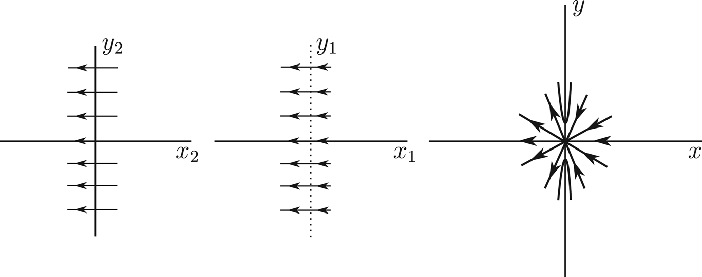
and rescaling the time $(x_2,\,y_2,\,t)\rightarrow (x_1,\,y_1,\,t/x_1^2)$ in (4.6), we obtain:

Going back through the changes of variables the local phase portrait at the equilibrium point (the origin) is shown in figure 1, if $a_{14}>0$ . When $a_{14}<0,$
 the local phase portrait of the origin is the one of figure 1, reversing the orientation of the orbits. So, when $a_{14}\ne 0,$
 there are orbits which go or come from the infinity in system (4.1), and consequently the centre of this system cannot be global. Assume now that $a_{14}=0$
 . Then, system (4.2) writes:

The infinite equilibrium points of this system are

if they exist. When they exist, since differential system (4.8) is invariant under the symmetry $(x,\,y,\,t)\to (-x,\,y,\,-t),$ we only need to study the local phase portrait at the infinite equilibrium point $\mathcal {P}_+$
 .
Here $a_{14}>0$ . In the left panel, there is the local phase portrait in a neighbourhood of the $y_2$
 -axis of systems (4.7). In the middle panel, there is the local phase portrait in a neighbourhood of the $y_2$
 -axis of system (4.6). The local phase portrait of the equilibrium point at the origin of the chart $U_2$
 is shown in the right panel.

We divide the study of the possible infinite singular points of system (4.8) into the following six cases:

$\bullet$ Case $c_1$
 . Then, translating the equilibrium $\mathcal {P}_+$
 to the origin, system (4.8) becomes $\dot {x}=2 a \sqrt {a_{32}}\, x+\cdots$
 , $\dot {y}=\cdots$
 , here the dots mean terms of degree higher than one in the variables $x$
 and $y.$
 Then, this equilibrium, by Theorem 2.15 of [Reference Dumortier, Llibre and Artés12], is a semi-hyperbolic saddle, or node, or saddle-node, and consequently some orbit of system (4.1) goes or comes from the infinity, and system (4.1) cannot have a global centre.
$\bullet$ Case $c_2$
 . Then, system (4.3) writes:

From (4.5) the characteristic direction at the origin is $\gamma _{4}=y^5=0$ , and we can do the vertical blow-up $(x,\,y)\rightarrow (x_1,\,y_1\,x_1),$
 without loosing information because $x=0$
 is not a characteristic direction. So, system (4.10) goes over the system:

and doing the rescaling of the time $(x_2,\,y_2,\,t)\to (x_1,\,y_1,\,t/x_1^3)$ in system (4.11), we get the system:

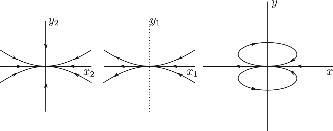
Then, the origin of this system is a stable semi-hyperbolic node (see Theorem 2.15 of [Reference Dumortier, Llibre and Artés12]), and going back through the changes of variables we obtain that the origin in the chart $U_2$ has an elliptic sector (see figure 2). Then, there are orbits of system (4.1) going to infinity. Hence, system (4.1) cannot have a global centre.
In the left panel, the origin ofsystem (4.12) is a semi-hyperbolic node. Inmiddle, for system (4.11), all points on the $y_1$ -axis are equilibrium points, and by rescaling the time in the left flow, and changing the direction concerning the previous one, and on the right the local phase portrait in the neighbourhood of the equilibrium point at the origin of system (4.10) has a nilpotent elliptic sector.

$\bullet$ Case $c_3$
 . Then, there are no infinite singular points in the local chart $U_1$
 . So, it is enough to study the origin of the local chart $U_2$
 . Now, system (4.3) is

Since $\gamma _{4}=y^5=0$ , we do the vertical blow-up $(x,\,y)\rightarrow (x_1,\,y_1\,x_1),$
 and system (4.13) becomes

and doing the rescaling $(x_2,\,y_2,\,t)\rightarrow (x_1,\,y_1,\, t/x_1^3)$ to system (4.14) we get:

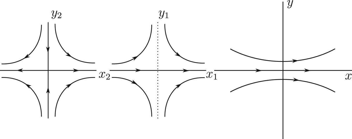
Thus, the origin of system (4.15) is a semi-hyperbolic saddle (by Theorem 2.15 of [Reference Dumortier, Llibre and Artés12]), see the left panel of figure 3. Going back to system (4.14), we obtain the phase portrait of the middle panel of figure 3. In that panel, the $y_1$ -axis is filled with equilibria. Undoing the vertical blow-up, we obtain the nilpotent hyperbolic sector at the origin of the local chart $U_2$
 corresponding to system (4.13) showing in the right panel of figure 3. Therefore, by proposition 2.2, in this case system (4.1) has a global centre.
Local phase portraits corresponding to the blow-up of the origin in the chart $U_2$ of system (4.13).

$\bullet$ Case $c_4$
 . For this case we have systems (4.13), (4.14), and (4.15) with $a=0$
 , and as in case $c_3,$
 the local phase portrait at the origin of the local chart $U_2$
 is shown in the right panel of figure 3. Now, we must study the local phase portrait at the origin of the local chart $U_1$
 . So, system (4.2) is

Since $\gamma _6=-y\,(y^4-a_{32}\,x^2)$ we can do the vertical blow-up $(x,\,y)\rightarrow (x_1,\,y_1\,x_1)$
 to system (4.16), and we obtain:

then with the rescaling $(x_2,\,y_2,\,t)\rightarrow (x_1,\,y_1,\,t/x_1)$ , system (4.17) writes:

Therefore, the origin of system (4.18) is a hyperbolic saddle, its phase portrait is the one of the left panel of figure 3, but with the orbit in the reverse sense. Going back through the changes of variables, we obtain that the local phase portrait at the origin of the local chart $U_1$ is the one of the right panel of figure 3, reversing the orientation of the orbits. So, again from proposition 2.2, in this case system (4.1) has a global centre.
$\bullet$ Case $c_5$
 . From (4.8) it follows that there are no infinite singular points in the local chart $U_1$
 . Hence, we must study only the origin of the local chart $U_2$
 . So, system (4.3) is

Since $\gamma _6=y^5$ , we do the vertical blow-up and after the rescaling of the time $(x,\,y,\,t)\rightarrow (x_1,\,y_1\,x_1,\,t/x_1^3),$
 and we obtain:

Now, $\gamma _5=a^2\,x_1^3\,y_1$ , therefore $x_1=0$
 is a characteristic direction and, before doing a vertical blow-up, we do the twist $(x_1,\,y_1)\rightarrow (x_2-y_2,\,y_2)$
 in system (4.20), and we get:

Since $\gamma _5=a^2\,y_2\,(x_2-y_2)^3$ , we do the vertical blow-up and the rescaling of the time $(x_2,\,y_2,\,t)\to (x_3,\,y_3\,x_3,\,t/x_3^2)$
 in system (4.21), so we obtain the system:

The equilibria of system (4.22) on the straight line $x_3=0$ are the origin and $(0,\,1)$
 . The origin is a hyperbolic saddle, and the $(0,\,1)$
 is linearly zero, i.e. the matrix of the linear part of system (4.22) is identically zero. Then, we will study the local phase portrait at the point $(0,\,1)$
 doing blow-up's. First, we translate the equilibrium point $(0,\,1)$
 to the origin of coordinates, so applying in (4.22) the change $(x_3,\,y_3)\rightarrow (x_4,\,y_4+1),$
 we get:

For system (4.23), we have $\gamma _5=-x_4\,y_4(3\,x_4^2+a^2\, y_4^2)$ , then $x_4=0$
 is a characteristic direction. Therefore, we do the twist $(x_4,\,y_4)\rightarrow (x_5-y_5,\,y_5)$
 to system (4.23), and after doing the vertical blow-up and the rescaling of the time $(x_5,\,y_5,\,t) \rightarrow (x_6,\,y_6\,x_6,\,t/x_6^2)$
 , we obtain the system:

where $f$ and $g$
 are polynomials of degrees $21$
 and $20$
 in the variables $x_6,\, y_6,$
 respectively.
From (4.24) we obtain that the equilibrium points on $y_6=0$ are the origin and $(0,\,1).$
 Both equilibria are hyperbolic saddles. Therefore, going back to system (4.22), we obtain the local phase portrait at the equilibrium $(0,\,1)$
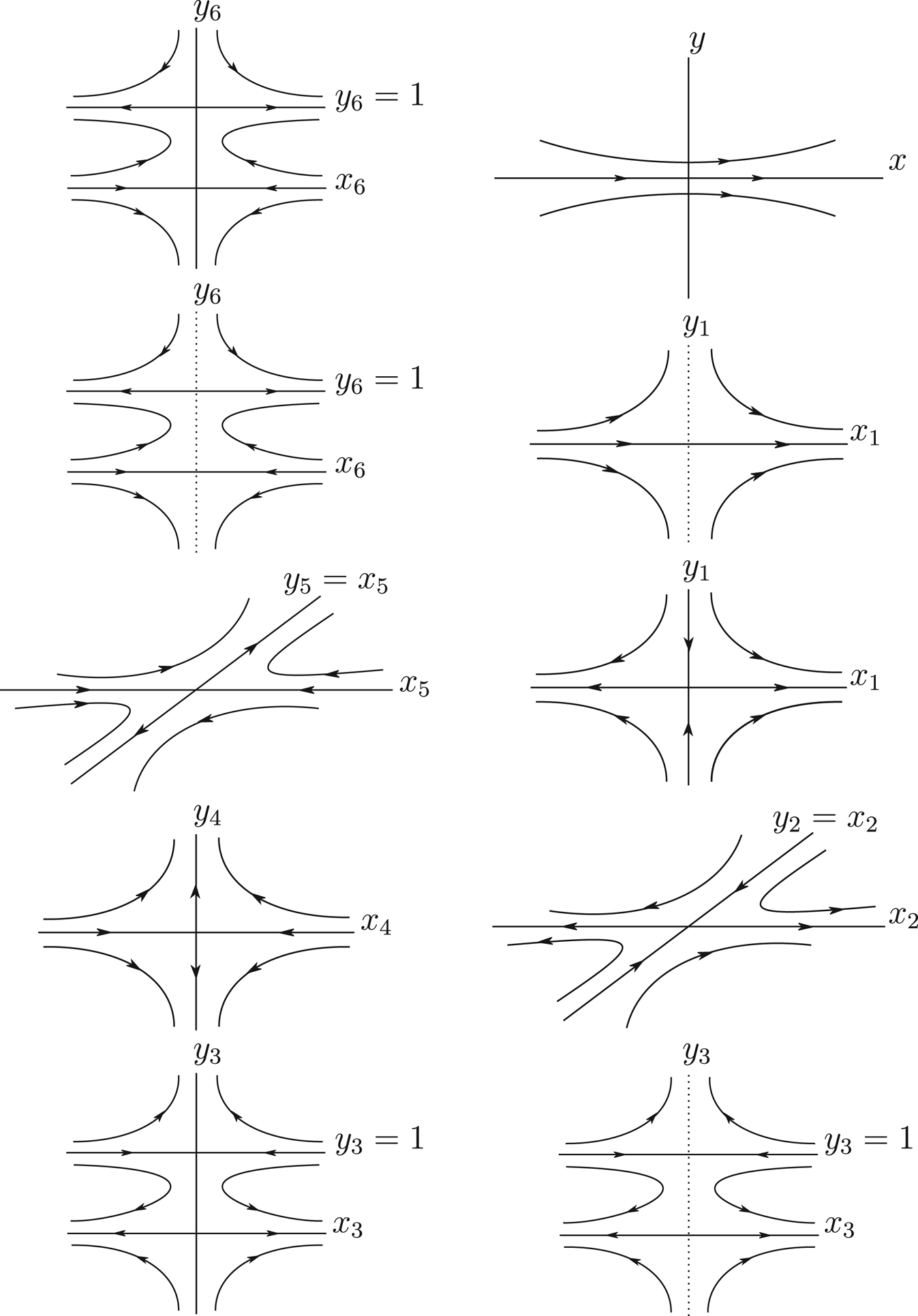
 . The steps on the blow down from differential system (4.24) up to system (4.22) are given in the left column of figure 4.
Local phase portrait corresponding to the blow-up of the origin of the chart $U_2$ of system (4.19). Starting with the top panel on the left column, then going down one by one in the left column: the local phase portrait of system (4.24), both equilibrium points the origin and $(0,\,1)$
 are hyperbolic saddles. In the next one all points on $y_6$
 -axis are equilibrium points. Undoing the blow-up we obtain a saddle for system $(\dot x_5,\,\dot y_5)$
 , and undoing the twist transformation we continue having a saddle for system $(\dot x_4,\,\dot y_4)$
 .

Finally, going back to differential system (4.19), we get the local phase portraits at the origin of the chart $U_2$ . The different steps of this blow down are in the right column of figure 4. Again, in this case from proposition 2.2 differential system (4.1) has a global centre.
$\bullet$ Case $c_6$
 . Then, differential system (1.3) under the conditions of theorem 1.1 becomes the linear differential system $\dot x=y$
 . $\dot y=-x$
 .
In summary, from cases $c_3$ , $c_4$
 , and $c_5,$
 it follows the proof of theorem 1.2.
In the following we get for system $(\dot x_3,\,\dot y_3)$ two saddles: one hyperbolic at the origin and one linearly zero at $(0,\,1)$
 . Now, at the end of the right column, undoing the time rescaling we obtain the same local phase portrait in a neighbourhood of $y_3=0$
 with the exception that the straight line $y_3=0$
 is filled with equilibrium points. Undoing the blow-up, the twist transformation, the first rescaling and the first blow-up we obtain that the origin of $U_2$
 is formed by two hyperbolic sectors having their separatrices on the infinite circle.
Acknowledgements
The first author is supported by Sáo Paulo Research Foundation (FAPESP) grants number 2022/14484-9 and 2021/14987-8. The second author is partially supported by the Agencia Estatal de Investigación grant PID2019-104658GB-I00, the H2020 European Research Council grant MSCA-RISE-2017-777911, AGAUR (Generalitat de Catalunya) grant 2021SGR00113, and by the Acadèmia de Ciències i Arts de Barcelona.