1. Introduction
The stochastic model considered in this paper is a generalization of the stacked contact process introduced in [Reference Court, Blythe and Allen2] and studied analytically in [Reference Lanchier and Zhang10]. The stacked contact process is a spatial stochastic process based on the framework of interacting particle systems that describes the co-evolution of a population of hosts together with their symbionts. Individuals are located on the d-dimensional integer lattice and interact with their nearest neighbors. The model assumes that the symbionts can only live in association with their host (obligate relationship) and are transmitted both vertically from associated hosts to their offspring and horizontally from associated hosts to nearby unassociated hosts. The stacked contact process [Reference Court, Blythe and Allen2, Reference Lanchier and Zhang10] also assumes that all the hosts give birth and die at the same rate regardless of whether they are associated with a symbiont or not, meaning that the symbionts have no effect on the fitness of their host. This paper considers the natural generalization of the stacked contact process in which associated and unassociated hosts have different birth rates: symbionts that increase the birth rate of their host, and therefore have a beneficial effect, are referred to as mutualists, whereas symbionts that decrease the birth rate of their host, and therefore have a detrimental effect, are referred to as pathogens. Formally, the state of the system at time t is a spatial configuration
 \begin{equation*} \xi_t \,:\, {\mathbb{Z}}^d \longrightarrow \{0, 1, 2 \} \end{equation*}
where state 0 means empty, state 1 means occupied by an unassociated host, and state 2 means occupied by a host associated with a symbiont. Letting
 \begin{equation*} \begin{array}{l} f_i (x, \xi) = (1/2d) \,\mathrm{card} \, \{y \in {\mathbb{Z}}^d \,:\, \sum_{j = 1, 2, \ldots, d} |x_j - y_j| = 1 \ \hbox{and} \ \xi (y) = i \} \end{array} \end{equation*}
be the fraction of nearest neighbors of vertex x which are in state i, hosts and symbionts co-evolve according to the spin system whose transition rates at vertex x are given by
 \begin{equation} \begin{array}{rclc@{\quad}rcl} 0 \ \to \ 1 & \quad\hbox{at rate} & \quad\lambda_{10} \,f_1 (x, \xi), & \quad & 1 \ \to \ 0 & \quad\hbox{at rate} & \quad 1, \\[5pt]
0 \ \to \ 2 & \quad\hbox{at rate} & \quad\lambda_{20} \,f_2 (x, \xi), & \quad & 2 \ \to \ 0 & \quad\hbox{at rate} & \quad 1, \\[5pt]
1 \ \to \ 2 & \quad\hbox{at rate} & \quad\lambda_{21} \,f_2 (x, \xi), & \quad & 2 \ \to \ 1 & \quad\hbox{at rate} & \quad\delta. \end{array}\end{equation}
The first four transition rates indicate that unassociated hosts give birth at rate  $\lambda_{10}$
, hosts associated with a symbiont give birth at rate
 $\lambda_{20}$
, and, regardless of whether they are associated or not, all the hosts die at the normalized rate one. An offspring produced at x is sent to a vertex chosen uniformly at random among the nearest neighbors, but the birth is suppressed when the target site is already occupied, which models competition for space. The offspring is always of the same type as its parent, indicating that the symbiont is always transmitted vertically. The process described by these four transitions is the multitype contact process [Reference Neuhauser13]. The effect of the symbiont on the host is modeled by the choice of the two birth rates: the symbiont is
 \begin{equation*} \begin{array}{rcl} \hbox{a pathogen} & \quad\hbox{when} & \quad\lambda_{20} \lt \lambda_{10} , \\[5pt]
\hbox{a mutualist} & \quad\hbox{when} & \quad\lambda_{20} \gt \lambda_{10}. \end{array} \end{equation*}
The last two transitions describe the symbiont dynamics within the host population. The symbiont spreads to adjacent unassociated hosts at rate  $\lambda_{21}$
, which corresponds to a horizontal transmission of the symbiont. Finally, hosts associated with a symbiont become unassociated at rate
 $\delta$
, which we simply call the recovery rate even when the symbiont is a mutualist.
The stacked contact process [Reference Court, Blythe and Allen2, Reference Lanchier and Zhang10] is obtained by setting  $\lambda_{20} = \lambda_{10}$
. This corresponds to the neutral case in which the symbionts have no effect on the fertility of their hosts, i.e. all the hosts have the same birth rate. The analysis of this special case in [Reference Lanchier and Zhang10] is somewhat facilitated by the fact that the process is attractive and monotone with respect to its parameters. This is true in certain cases when
 $\lambda_{10} \neq \lambda_{20}$
, but not always; for example, it is false in the setting of Theorem 3.
1.1. Mean-field approximation
Before studying the spatial stochastic process, we first look at its non-spatial deterministic counterpart called mean-field approximation, consisting of a pair of coupled ordinary differential equations. We give a derivation and a brief summary of its properties; the reader may consult [Reference Foxall6] for a thorough treatment. To derive it, consider a set of N sites each of which can be either empty, occupied by an unassociated host, or occupied by an associated host. We suppose that each unassociated host attempts to give birth to an unassociated host onto a site chosen uniformly at random at rate  ${\lambda}_{10}$
, being successful if that site is empty. Similarly, each associated host attempts to give birth to an associated host at rate
 ${\lambda}_{20}$
. Each host dies at rate 1, while each symbiont dies (i.e. each associated host becomes an unassociated host) at rate
 $\delta$
. Each associated host attempts to transmit the symbiont to a randomly chosen site at rate
 ${\lambda}_{21}$
, being successful if the recipient is an unassociated host. Letting
 $U(t) = (U_0(t),U_1(t),U_2(t))$
denote the number of empty sites, unassociated hosts, and associated hosts, respectively, and rescaling to
 $u = U/N$
, we have the Markov chain with transitions
 \begin{align*} &u \to u + N^{-1}(\!-1,1,0) \hbox{ at rate } N {\lambda}_{10} \,u_0u_1, \qquad u \to u + N^{-1}(1,-1,0) \hbox{ at rate } N u_1, \\ &u \to u + N^{-1}(\!-1,0,1) \hbox{ at rate } N {\lambda}_{20} \,u_0u_2, \qquad u \to u + N^{-1}(1,0,-1) \hbox{ at rate } N u_2, \\ &u \to u + N^{-1}(0,-1,1) \hbox{ at rate } N {\lambda}_{21} \,u_1u_2, \qquad\ u \to u + N^{-1}(0,1,-1) \hbox{ at rate } N \delta \,u_2. \end{align*}
This shows that u is a density-dependent Markov chain in the sense of [Reference Kurtz9]. Since the three densities add up to one, instead let  $u = (u_1, u_2)$
. Writing
 $u^N$
to emphasize the dependence on N, if
 $\lim_{N \to \infty} u^N(0) = u$
and
 ${\varepsilon},T \gt 0$
, it follows from Theorem 2.2 in [Reference Kurtz9] that
 \begin{equation*} \lim_{N\to\infty} {\rm P} \Big(\sup_{t \le T}|u^N(t) - u(t)| \gt {\varepsilon} \Big) = 0, \end{equation*}
where u(t) is the solution to the initial value problem  $u(0) = u$
, and
 \begin{equation} \begin{array}{r@{\,}c@{\,}l} u_1^{\prime} & = & \,{\lambda}_{10} \,u_0 u_1 - u_1 + \delta u_2 - {\lambda}_{21} \,u_1 u_2 , \\[5pt]
u_2^{\prime} & = & \,{\lambda}_{20} \,u_0 u_2 - u_2 - \delta u_2 + {\lambda}_{21} \,u_1 u_2. \end{array}\end{equation}
It turns out to be more productive to study the proportion of hosts,  $x_1 = u_1 + u_2$
, and the proportion of hosts that are associated,
 $x_2 = u_2/x_1$
. Letting
 \begin{equation*} {\lambda}_a = {\lambda}_{20} - {\lambda}_{10} \quad \hbox{and} \quad {\lambda}_b = -{\lambda}_a + {\lambda}_{21}, \end{equation*}
after a bit of algebra we obtain the system
 \begin{equation}\begin{array}{rcl} x_1^{\prime} & = & \,G_1 (x_1,x_2) = x_1 \,(({\lambda}_{10} + {\lambda}_a x_2)(1-x_1) - 1) , \\[5pt]
x_2^{\prime} & = & \,G_2 (x_1,x_2) = x_2 \,(({\lambda}_a + {\lambda}_b x_1)(1-x_2) - \delta).\end{array}\end{equation}
Note that the map  $(u_1,u_2)\mapsto(x_1,x_2)$
is undefined at
 $x_1=0$
, but the inverse
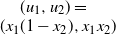 $(u_1,u_2)=\break (x_1(1-x_2),x_1x_2)$
is smooth and maps solutions of (3) to solutions of (2). Define the set of interest
 $\Lambda = [0, 1]^2$
and
 \begin{equation*} {\Lambda}_+ = \begin{cases} (0, 1] \times (0, 1) = \{(x_1, x_2) \in {\Lambda} \,:\, x_1>0, \ 0 <x_2<1 \} & \hbox{if} \ \delta = 0, \\[5pt]
(0, 1] \times (0, 1] = \{(x_1, x_2) \in {\Lambda} \,:\, x_1,x_2 \gt 0 \} & \hbox{if} \ \delta \gt 0,\end{cases} \end{equation*}
which is obtained by removing invariant lines on the boundary of  ${\Lambda}$
. In addition, let
 \begin{equation*}\begin{array}{ll} p_0=(0,0), & \quad p_1 = (a_1, 0) = (1 - 1/{\lambda}_{10}, 0), \\[5pt] p_2 = (a_2,1) = (1-1/{\lambda}_{20},1), & \quad p_3 = (0, a_3) = (0,1-\delta/{\lambda}_a). \end{array}\end{equation*}
Except for very specific parameter values, these are the only candidates for equilibria on the boundary of  ${\Lambda}$
. We also define two conditions on the parameters:
 \begin{equation*}\begin{array}{cl} \hbox{(AinvU)}: & \quad{\lambda}_{20}(1-a_1) + {\lambda}_{21}a_1 \gt 1 + \delta , \\[5pt]
\hbox{(UinvA)}: & \quad{\lambda}_{10}(1-a_2) - {\lambda}_{21}a_2 \gt 1. \end{array} \end{equation*}
The meaning of these two conditions is as follows:
• (AinvU) stands for ‘associated invades unassociated’, and is relevant if and only if
 $\lambda_{10} \gt 1$
. It corresponds to parameter values for which a small introduction of associated hosts in a stable population of unassociated hosts leads to an increase in the proportion of associated hosts. It is equivalent to
$G_2 (p_1 + {\varepsilon} e_2) \gt 0$
for small
${\varepsilon} \gt 0$
, where
$e_2 = (0, 1)$
.
• (UinvA) stands for ‘unassociated invades associated’, and is relevant if and only if
${\lambda}_{20}>1$
and
$\delta=0$
. It corresponds to parameter values for which a small introduction of unassociated hosts in a stable population of associated hosts leads to an increase in the proportion of unassociated hosts. It is equivalent to
$G_1(p_2 + {\varepsilon} e_2) >0$
for small
${\varepsilon}>0$
, where
$e_1=(1,0)$
.







For  $x \in {\Lambda}$
let
 $t\mapsto \phi(t,x)$
denote the solution to (3) with initial value x. The following result is proved in the companion paper [Reference Foxall6]. We omit some details in the bistability case, since it is not the focus here.
Theorem 1. The following six cases include all parameter values.
There are two special cases.
1. Redundant symbiont (RS): Suppose
$\max ({\lambda}_{10}, {\lambda}_{20}) \gt 1$
and
$\delta = {\lambda}_a = {\lambda}_{21} = 0$
. For all
$x \in {\lambda}_+$
,
$\lim_{t \to \infty} \phi_1 (t, x) = a_1$
and
$t\mapsto \phi_2 (t, x)$
is constant.2. Bistability (B): There may be up to two locally stable equilibria. This occurs for some, but not all, parameter values satisfying
$\min ({\lambda}_a, {\lambda}_b) \gt 0$
and either (i)
${\lambda}_{10}\le 1 \lt {\lambda}_{20} \lt 1+\delta$
, or(ii)
${\lambda}_{10}>1$
and (AinvU) does not hold.








Suppose (RS) and (B) do not hold. Then there exists  $\bar x \in {\Lambda}$
such that
 $\lim_{t \to \infty} \phi(t, x) =\bar x$
for all
 $x \in {\Lambda}_+$
. Assuming (RS) and (B) do not hold, four cases are possible.
1. Extinction (E):
$\bar x = (0,\max(0,a_3))$
if
${\lambda}_{10}\le 1$
and
${\lambda}_{20} \le 1+\delta$
.2. Survival and coexistence of associated and unassociated host (C):
in the following cases:
\begin{equation*} \max(0,\min(a_1,a_2)) \lt \bar x_1 \lt \max(a_1,a_2) \quad and \quad \max(0,a_3) \lt \bar x_2
< 1 \end{equation*}
(a)
$\delta>0$
and either (i)
${\lambda}_{10}\le 1$
and
${\lambda}_{20}>1+\delta$
, or(ii)
${\lambda}_{10}>1$
and (AinvU) holds; or
(b)
$\delta=0$
and either (i)
${\lambda}_{10}\le 1$
,
${\lambda}_{20}>1$
, and (UinvA) holds,(ii)
${\lambda}_{10}>1$
,
${\lambda}_{20}\le 1$
, and (AinvU) holds, or(iii)
$\min({\lambda}_{10},{\lambda}_{20})>1$
, (AinvU) holds, and (UinvA) holds.
3. Survival of unassociated host only (UH):
$\bar x = p_1$
if
${\lambda}_{10}>1$
and (AinvU) does not hold.4. Survival of associated host only (AH):
$\bar x = p_2$
if
$\delta=0$
,
${\lambda}_{20}>1$
, and (UinvA) does not hold.






Before continuing we make a couple of observations concerning this result. First of all, (RS) occurs only for a single choice of parameters. Moreover, (B) occurs only when we have  ${\lambda}_a>0$
and
 ${\lambda}_b>0$
, which corresponds to a mutualist whose rate of spread through the population exceeds the increase it provides to the host birth rate. Aside from (RS) and (B), four behaviors are possible: the host goes extinct (and thus also the symbiont) (E), the host survives but not the symbiont (UH), both host and symbiont survive with coexistence of associated and unassociated hosts (C), or the host survives and the symbiont spreads completely through the host population (AH). In each case, the conditions are straightforward: extinction occurs if the birth rate is too low, hosts survive without symbiont if the symbiont cannot invade the host in equilibrium, etc.
1.2. Spatial stochastic process
We can show that the spatial stochastic process exhibits the four main regimes identified above for the mean-field equations. Notice that another way to describe these four regimes is as follows: both unassociated hosts (type 1) and associated hosts (type 2) can either survive or go extinct. Since, for an interacting particle system, there is more than one notion of survival, we distinguish the two notions that we use. Single-site survival of type i means that, for some initial configuration  $\xi$
with a positive and finite number of type-i individuals (or, if
 $i = 1$
and
 $\delta \gt 0$
, at least one occupied site),
 \begin{equation*} {\rm P} (\hbox{for all} \ t \gt 0, \hbox{there exists} \ x \ \hbox{such that} \ \xi_t (x) = i \mid \xi_0 = \xi) \gt 0.\end{equation*}
The other notion of survival of type i, that we call global survival, is that starting from a translation-invariant distribution that almost surely has infinitely many type-i individuals,
 \begin{equation*} \liminf_{t \to \infty} \,{\rm P} (\xi_t (x) = i) \gt 0 \quad \hbox{for all} \quad x \in {\mathbb{Z}}^d.\end{equation*}
For the basic contact process discussed below, these two notions are known to coincide, a fact that follows from the model’s self-duality (see [Reference Liggett11] for details). Note that when the recovery rate  $\delta \gt 0$
, survival of associated hosts implies coexistence of associated and unassociated hosts.
As noted above, the stacked contact process obtained by setting  $\lambda_{10} = \lambda_{20}$
has several nice properties, including attractiveness and monotonicity as defined below. When
 ${\lambda}_{10} \ne {\lambda}_{20}$
it is still possible to have these properties, but only in certain cases. In this article we are not focused on the parameter regimes where attractiveness and monotonicity are present, except in the simpler subcases where an easy comparison to an already-studied process can be used. For the sake of the interested reader who wishes to make a further study of this process, we note, without proof, some other cases, not considered in detail in this article, for which we have some monotonicity.
Recall that a process is attractive with respect to a partial order on the set of configurations if, for any two configurations  $\xi \leq \xi^{\prime}$
, there exists a coupling of two processes
 $\xi_t, \xi_t^{\prime}$
with
 \begin{equation*} {\xi_0 = \xi , \quad \xi_0^{\prime} = \xi^{\prime} , \quad \hbox{and} \quad \xi_t \leq \xi_t^{\prime} \qquad \hbox{for all } t \gt 0.} \end{equation*}
A process is monotone increasing with respect to a parameter  $\rho$
if the above property holds when
 $\xi_t,\xi_t^{\prime}$
have respective parameter values
 $\rho \le \rho'$
, and monotone decreasing if
 $\rho \ge \rho'$
. We focus on partial orders induced by a sitewise order on types, that is,
 \begin{equation*} \xi \leq \xi' \quad \hbox{if and only if} \quad \xi(x) \leq \xi'(x) \qquad \hbox{for all } x \in {\mathbb{Z}}^d. \end{equation*}
1.
${\lambda}_{10}>{\lambda}_{20}$
.
(a)
${\lambda}_{21}=0$
. Attractive for the partial order
$0,2<1$
and monotone increasing in
${\lambda}_{10},\delta$
.(b)
${\lambda}_{21}>0$
. Not attractive for any partial order with
$0<1$
.
2.
${\lambda}_{20}>{\lambda}_{10}$
.
(a)
${\lambda}_{20}>{\lambda}_{21}$
.
i.
$\delta>0$
. Not attractive for any partial order with
$0<2$
.ii.
$\delta=0$
. Attractive for the partial order
$0,1<2$
and monotone increasing in\break
${\lambda}_{20},{\lambda}_{21}$
.
(b)
${\lambda}_{20}={\lambda}_{21}$
. Type-2 sites give the basic contact process (described below) with birth rate
${\lambda}_{20}$
and death rate
$1+\delta$
.(c)
${\lambda}_{21}>{\lambda}_{20}$
. Attractive for the order
$0<1<2$
, monotone increasing in
${\lambda}_{10},{\lambda}_{20},{\lambda}_{21}$
, and monotone decreasing in
$\delta$
.


Our first result is obtained by comparing the stacked contact process with well-known interacting particle systems. More precisely, we will start by comparing the process with the basic contact process and the multitype contact process using simple coupling techniques. We will also show that the process inherits some of the properties of the forest fire model, though, because of the lack of monotonicity, this does not simply follow from a standard coupling argument. To state our result, we let  $\lambda_{\rm c} \in (0, \infty)$
be the critical value of the basic contact process.
Theorem 2. In all spatial dimensions,
 \begin{equation}
\phantom{the.}the\ hosts\ survive\ globally \quad when \quad \min \,(\lambda_{10}, \lambda_{20}) \gt \lambda_{\rm c},\end{equation}
 \hspace*{52pt}\begin{equation}
the\ hosts\ die\ out \quad when \quad \max \,(\lambda_{10}, \lambda_{20}) \leq \lambda_{\rm c},\hspace*{-52pt}
\end{equation}
 \begin{equation}
the\ associated\ hosts\ survive\ globally \quad when \quad \min \,(\lambda_{20}, \lambda_{21}) \gt (1 + \delta) \,\lambda_{\rm c},\end{equation}
 \hspace*{50pt}\begin{equation}
the\ associated\ hosts\ die\ out \quad when \quad \max \,(\lambda_{20}, \lambda_{21}) \leq (1 + \delta) \lambda_{\rm c}. \hspace*{-36pt}\end{equation}
In addition, in two dimensions,
 \begin{equation} \phantom{allyof th}the\ associated\ hosts\ die\ out \quad when \quad \lambda_{10} \gt \lambda_{20} \ \hbox{and} \ \lambda_{21}, \delta \ are\ small, \end{equation}
 \begin{equation} the\ associated\ hosts\ survive\ globally \quad when \quad \lambda_{20} \gt (1 + \delta) \,\alpha_c \ \hbox{and}\ \lambda_{10} \ is\ small. \end{equation}
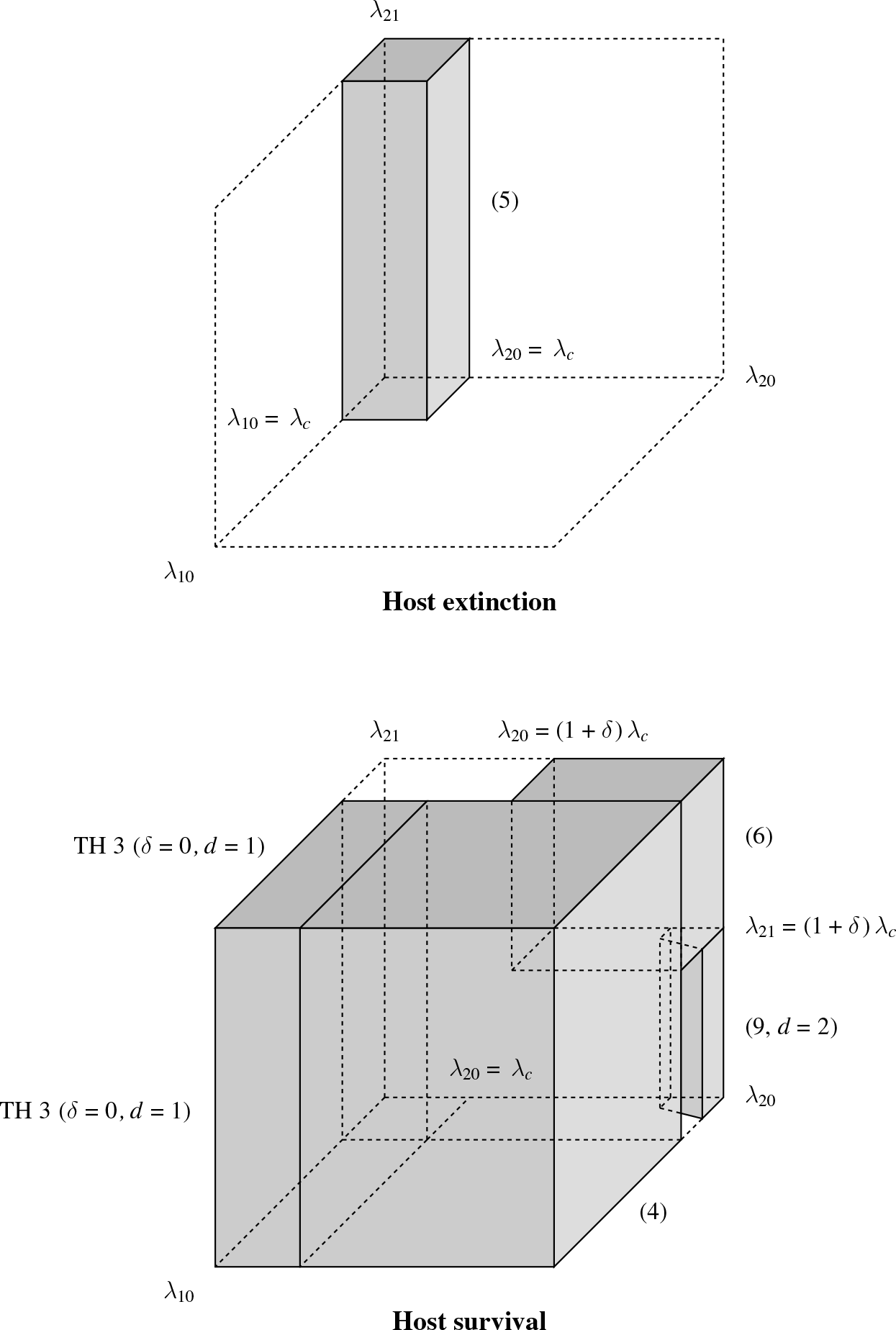
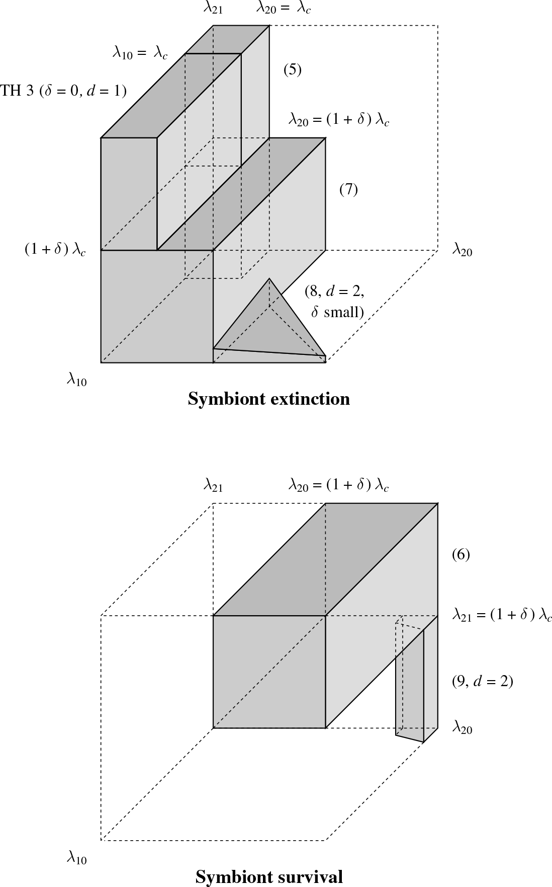
The parameter regions in (4)–(9) are shown in Figures 1 and 2. Note that the behavior of the stochastic process in the parameter regions (4)–(7) agrees with the behavior of its mean-field approximation described in Theorem 1, if we think of the mean-field model as having critical value  $\lambda_{\rm c} = 1$
. Indeed, observe for instance that
 \begin{equation*} \min \,(\lambda_{20}, \lambda_{21}) \gt 1 + \delta \quad \hbox{implies} \quad \hbox{(AinvU)}. \end{equation*}
The behavior in the parameter region (8) also agrees with the mean-field equations. To see this, notice that if  ${\lambda}_{10} \gt {\lambda}_{20}$
are fixed and
 ${\lambda}_{21} = \delta = 0$
then (AinvU) reduces to
 ${\lambda}_{20}/{\lambda}_{10} \gt 1$
, which does not hold, so (AinvU) still does not hold if
 $\delta,{\lambda}_{21}>0$
are small. Since
 ${\lambda}_{10}>{\lambda}_{20}$
, (B) does not hold and (RS) does not hold, so we have either (E) or (UH), depending on the values of
 ${\lambda}_{10}$
. In either case, Theorem 1 gives
 $x_2 \to 0$
so associated hosts do not persist.
We now focus on the parameter region where  $\lambda_{10} \gt \lambda_c \gt \lambda_{20}$
, which is not covered by the previous comparison results. In this case, the symbiont is a pathogen. Standard coupling arguments to compare the host–pathogen system with the basic contact process imply that a population of healthy (unassociated) hosts survives, whereas, if the recovery rate
 $\delta = 0$
, a population of infected (associated) hosts dies out. The long-term behavior when starting with a mixture of healthy and infected hosts is not clear, and the main question is whether associated and unassociated hosts coexist.
Theorem 1 says that in the mean-field model they do coexist provided  $\lambda_{21}$
is taken sufficiently large. For the spatial model, if the pathogen is to survive then, intuitively speaking, a certain proportion of infected hosts must remain in close contact with healthy hosts, since infected hosts alone will not survive. On the other hand, healthy hosts must also have room to spread into uninfected regions. This suggests that coexistence is favored in higher dimensions, where interaction neighborhoods involve more sites and each type has more room to move around. We are unable to show coexistence in higher dimensions, and indeed, few results of this type exist in the literature. A recent example is [Reference Moore, Morters and Rogers12], which treats a stacked SIR model on the Erdos–Renyi graph and shows that survival of the secondary infection is favored by intermediate rates of spread in the primary infection. However, in our case recovery is not permanent and the interaction graph (a lattice) is not locally tree-like, both of which significantly complicate the model.
On the other hand, we are able to show that, in one dimension, when  $\delta = 0$
and even when the infection rate and the birth rate of healthy hosts are very large, the pathogen is unable to survive.
Theorem 3. Assume that  $\lambda_{10} \gt \lambda_c \gt \lambda_{20}$
,
 $\delta = 0$
, and
 $d = 1$
. Then, starting from any configuration with infinitely many vertices in state 1,
 \begin{equation*} \liminf_{t \to \infty} \,{\rm P} (\xi_t (x) = 1) \gt 0 \quad \hbox{and} \quad \lim_{t \to \infty} \,{\rm P} (\xi_t (x) = 2) = 0 \qquad\ {for\ all}\ x \in {\mathbb{Z}}. \end{equation*}
Picture of the parameter region (5) in which the host is known to die out, at the top, and of the parameter regions (4), (6), (9), and the one in Theorem 3 in which the host is known to survive, at the bottom. Note that the bottom picture accounts for the fact that how small  $\lambda_{10}$
is in (9) might depend on the value of
 $\lambda_{20}$
.
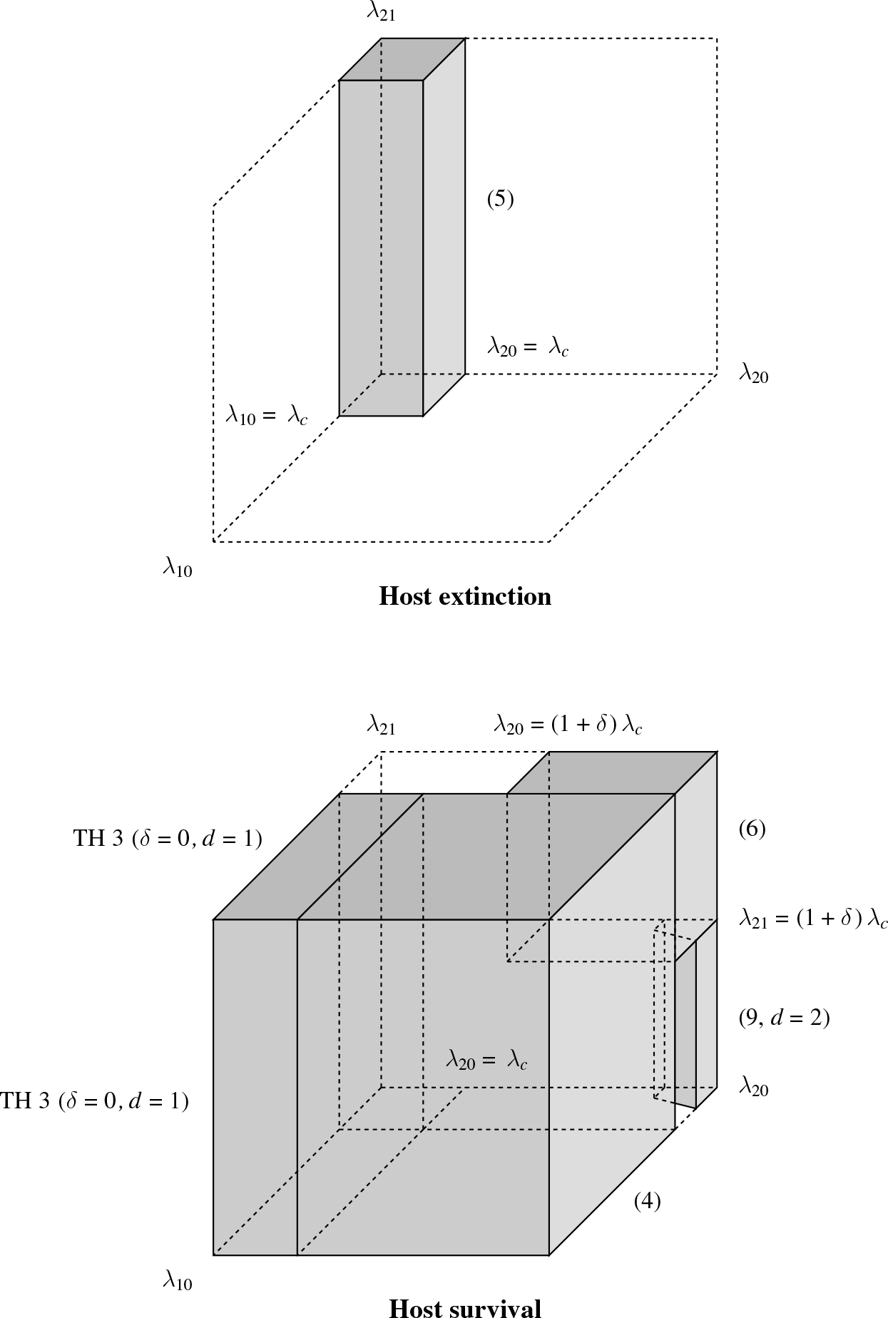
Picture of the parameter regions (5), (7), (8), and the one in Theorem 3 in which the symbiont is known to die out, at the top, and of the parameter regions (6) and (9) in which the symbiont is known to survive, at the bottom. The pictures account for the fact that how small  $\lambda_{21}$
is in (8) might depend on the values of
 $\lambda_{10}$
and
 $\lambda_{20}$
, and how small
 $\lambda_{10}$
is in (9) might depend on
 $\lambda_{20}$
.
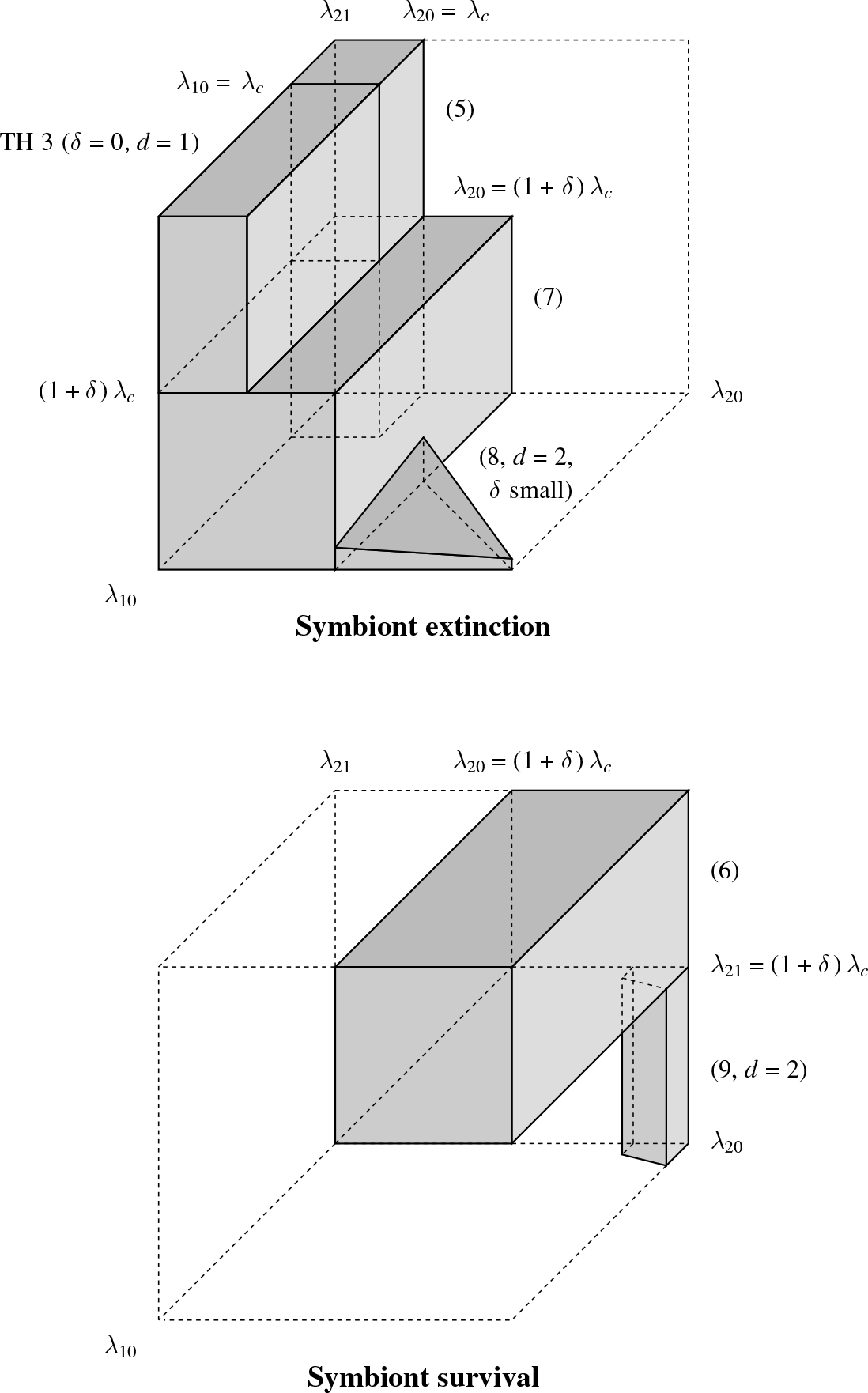
The parameter region covered in Theorem 3 is illustrated in the phase diagrams of Figures 1 and 2. Also, in addition to the statement of the theorem, our proof gives specific estimates on the rate of extinction of the pathogens and the rate of expansion of the healthy hosts. The first part of the proof shows that there exists a constant  $c \gt 0$
such that, uniformly in all initial configurations
 $\xi_0$
with infinitely many 1s and for any site x,
 \begin{equation} {\rm P} (\!\sup \,\{t \,:\, \xi_t (y) = 2 \ \hbox{for some} \ y \ \hbox{such that} \ |y - x| \leq \e^{ct} \} \lt \infty) = 1.\end{equation}
In other words, there exists a uniform (over all sites) exponentially growing (in time) neighborhood of any site which is eventually void of pathogens. To describe the long-term behavior of the healthy hosts, let  $\zeta_t$
denote the one-dimensional nearest-neighbor (supercritical) contact process with parameter
 $\lambda_{10}$
starting from the all-one configuration. Also, let
 $\alpha \gt 0$
denote the edge speed in this contact process as defined in [Reference Durrett3]; that is, starting from the initial configuration
 $\xi_0 (x) = {\mathbf{1}} \{x \le 0 \}$
,
 \begin{equation*}\alpha = \lim_{t\to\infty}t^{-1}\sup\{x\,{:}\,\xi_t(x) \ne 0\}.\end{equation*}
Then, under the assumptions of the theorem, there exist
• a random site X and an almost surely finite time T that depend on
$\xi$
,• site-valued processes
$\ell_t \leq r_t$
defined for
$t \geq T$
and satisfying
$\ell_T = r_T = X$
,• a coupling of the processes
$\xi_t$
and
$\zeta_t$


such that, P-almost surely,
 \begin{equation} \lim_{t \to \infty} - \ell_t / t = \lim_{t \to \infty} r_t / t = \alpha \quad \hbox{and} \quad \xi_t (x) = \zeta_t (x) \ \hbox{for all} \ (x, t) \in [\ell_t, r_t] \times [T, \infty). \end{equation}
In other words, as long as  $\xi$
has an infinite number of 1s, then, P-almost surely, eventually there arises a stable population of 1s that behaves like the basic contact process on an interval that grows linearly in time. From (10) and (11), we also obtain a complete convergence theorem. Indeed, letting
 $\nu$
denote the upper invariant measure of the contact process
 $\zeta_t$
and
 $\delta_0$
denote the measure that concentrates on the all-zero configuration, since the distribution of the contact process converges weakly to
 $\nu$
[Reference Liggett11, Ch. VI], we deduce the following for the distribution
 $\mu_t$
of the process
 $\xi_t$
.
Corollary 1. Let  $\lambda_{10} \gt \lambda_c \gt \lambda_{20}$
,
 $\delta = 0$
, and
 $d = 1$
. Then, as
 $t \to \infty$
,
 \begin{equation*} \mu_t \Rightarrow \rho \delta_0 + (1 - \rho) \nu \quad \hbox{where} \quad \rho = {\rm P}_{\mu_0} (\{x \,:\, \xi_t (x) = 1 \}\neq \varnothing \ \hbox{for all} \ t \gt 0). \end{equation*}
In particular, all invariant measures are convex combinations of  $\delta_0$
and
 $\nu$
.
2. Proof of Theorem 2
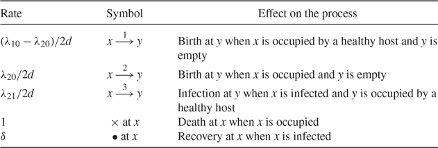
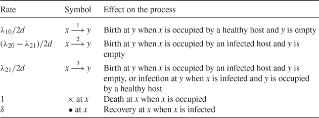
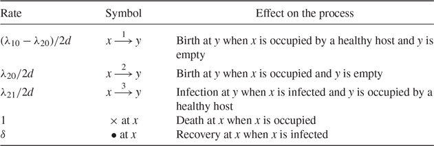
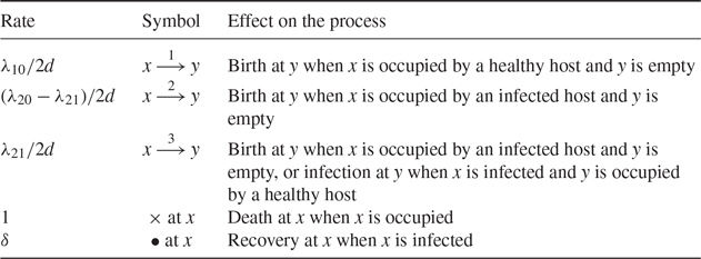
Throughout the paper, we think of the process as being generated from a percolation substructure, also called Harris’ graphical representation [Reference Harris8]. The percolation substructure consists of independent Poisson processes with appropriate rates attached to each vertex and oriented edge of the d-dimensional integer lattice. The process is then constructed by assuming that, at the times of these Poisson processes, either a birth, or an infection, or a death, or a recovery occurs whenever the configuration of the system at that time is compatible with the event. Table 1 shows, for instance, how the stacked contact process can be constructed when  $\lambda_{10} \geq \lambda_{20}$
, while Table 2 shows another example of contruction when
 $\lambda_{20} \geq \lambda_{21}$
.
Graphical representation of the process when  $\lambda_{10} \geq \lambda_{20}$
(pathogen). The rates in the left column correspond to the different parameters of the independent Poisson processes, attached to either each oriented-edge-connected two neighbors (first three rows) or each vertex (last two rows).
Graphical representation of the process when  $\lambda_{20} \geq \lambda_{21}$
. The rates in the left column correspond to the different parameters of the independent Poisson processes, attached to either each oriented-edge-connected two neighbors (first three rows) or each vertex (last two rows).
Proof of (4)–(7). In the limiting case when the recovery rate  $\delta = \infty$
, all the symbionts die instantaneously so the host dynamics reduces to the basic contact process
 \begin{equation*} \begin{array}{r@{\quad}c@{\quad}l@{\quad}c@{\quad}r@{\quad}c@{\quad}l} 0 \ \to \ 1 & \hbox{at rate} & \lambda_{10} \,f_1 (x, \xi), & \quad & 1 \ \to \ 0 & \hbox{at rate} & 1. \end{array} \end{equation*}
In this case, there is a critical value  $\lambda_{\rm c} \in (0, \infty)$
such that above
 $\lambda_{\rm c}$
the host population survives whereas at and below
 $\lambda_{\rm c}$
the population goes extinct [Reference Bezuidenhout and Grimmett1]. This is in qualitative agreement with the mean-field equations.
Assume from now on that the recovery rate is finite and let
 \begin{equation*} \xi_t^1 (x) = {\mathbf{1}} \{\xi_t (x) \neq 0 \} \quad \hbox{and} \quad \xi_t^2 (x) = {\mathbf{1}} \{\xi_t (x) = 2 \} \qquad \hbox{for all } x \in {\mathbb{Z}}^d \end{equation*}
be the process that keeps track of the hosts and the process that keeps track of the hosts associated to a symbiont, respectively. The transitions of the process  $\xi_t^1$
satisfy
 \begin{equation*} \begin{array}{r@{\quad}c@{\quad}r} 0 \ \to \ 1 & \hbox{at rate at least} & \min \,(\lambda_{10}, \lambda_{20})\quad f_1 (x, \xi^1) , \\[5pt] 0 \ \to \ 1 & \hbox{at rate at most} & \max \,(\lambda_{10}, \lambda_{20})\quad f_1 (x, \xi^1) , \end{array} \end{equation*}
while  $1 \to 0$
at rate one. In particular, this process can be compared to the basic contact process to deduce that, for all
 $x \in {\mathbb{Z}}^d$
and starting from a translation-invariant distribution with infinitely many 1s and 2s,
 \begin{equation*} \begin{array}{r@{\quad}c@{\quad}l} \displaystyle \liminf_{t \to \infty} \,{\rm P} (\xi_t (x) \neq 0) \gt 0 & \hbox{when} & \min \,(\lambda_{10}, \lambda_{20}) \gt \lambda_{\rm c} , \\ \\[-5pt] \displaystyle \lim_{t \to \infty} \,{\rm P} (\xi_t (x) \neq 0) = 0 & \hbox{when} & \max \,(\lambda_{10}, \lambda_{20}) \leq \lambda_{\rm c}. \end{array} \end{equation*}
This follows from Theorem III.1.5 in [Reference Liggett11], which applies to general two-state spin systems, together with obvious inequalities relating the transition rates of our process and their counterpart for the basic contact process. This proves (4) and (5). Alternatively, one can prove these results by using a coupling argument. For instance, when  $\lambda_{10} \geq \lambda_{20}$
, the contact process
 $\zeta_t^2$
with parameter
 $\lambda_{20}$
can be constructed from the graphical representation in Table 1 by assuming that births can only occur through type-2 arrows, while the contact process
 $\zeta_t^1$
with parameter
 $\lambda_{10}$
can be constructed by assuming that births occur through both type-1 and type-2 arrows. In both processes, particles are killed at the death marks
 $\times$
. Constructing the stacked contact process and these two contact processes from this common graphical representation results in a coupling such that
 \begin{equation*} \{x \in {\mathbb{Z}}^d \,:\, \zeta_t^2 (x) = 1 \} \subset \{x \in {\mathbb{Z}}^d \,:\, \xi_t^1 (x) = 1 \} \subset \{x \in {\mathbb{Z}}^d \,:\, \zeta_t^1 (x) = 1 \} \end{equation*}
at all times t, provided this holds at time zero. This shows (4) and (5) when  $\lambda_{10} \geq \lambda_{20}$
.
The analogous property when the inequality is reversed can be proved similarly by using another graphical representation which is designed based on the ordering of the parameters. Looking now at the second process  $\xi_t^2$
, the transitions satisfy
 \begin{equation*} \begin{array}{r@{\quad}c@{\quad}r} 0 \ \to \ 1 & \hbox{at rate at least} & \min \,(\lambda_{20}, \lambda_{21})\quad f_1 (x, \xi^2) , \\ \\[-5pt] 0 \ \to \ 1 & \hbox{at rate at most} & \max \,(\lambda_{20}, \lambda_{21})\quad f_1 (x, \xi^2) , \end{array} \end{equation*}
while  $1 \to 0$
at rate
 $1 + \delta$
, from which it follows that, for all
 $x \in {\mathbb{Z}}^d$
and starting from a translation-invariant distribution with infinitely many 1s and 2s,
 \begin{equation*} \begin{array}{r@{\quad}c@{\quad}l} \displaystyle \liminf_{t \to \infty} \,{\rm P} (\xi_t (x) = 2) \gt 0 & \hbox{when} & \min \,(\lambda_{20}, \lambda_{21}) \gt (1 + \delta) \,\lambda_{\rm c} , \\ \\[-5pt] \displaystyle \lim_{t \to \infty} \,{\rm P} (\xi_t (x) = 2) = 0 & \hbox{when} & \max \,(\lambda_{20}, \lambda_{21}) \leq (1 + \delta) \lambda_{\rm c}, \end{array} \end{equation*}
which shows (6) and (7). This can again be proved by using Theorem III.1.5 in [Reference Liggett11], or by coupling the process with the two contact processes with respective birth rates  $\lambda_{20}$
and
 $\lambda_{21}$
and common death rate
 $1 + \delta$
using the graphical representation in Table 2 when
 $\lambda_{20} \geq \lambda_{21}$
, while the analogous property when the inequality is reversed can be proved by using another graphical representation which is designed based on the ordering of the parameters.
The four parameter regions in (4)–(7) are illustrated in the diagrams of Figures 1 and 2.
Proof of (8). Setting  $\lambda_{21} = \delta = 0$
, the process reduces to the multitype contact process completely analyzed when the death rates are equal in [Reference Neuhauser13]. The transition rates become
 \begin{equation*} \begin{array}{r@{\quad}c@{\quad}l@{\quad}c@{\quad}r@{\quad}c@{\quad}l} 0 \ \to \ 1 & \hbox{at rate} & \lambda_{10} \,f_1 (x, \xi) , & \quad & 1 \ \to \ 0 & \hbox{at rate} & 1 , \\ \\[-5pt] 0 \ \to \ 2 & \hbox{at rate} & \lambda_{20} \,f_2 (x, \xi) , & \quad & 2 \ \to \ 0 & \hbox{at rate} & 1. \end{array} \end{equation*}
In this case, the type with the larger birth rate outcompetes the other type provided its birth rate is also strictly larger than the critical value of the single-type contact process. This result was first proved in [Reference Neuhauser13] using duality techniques and again in [Reference Durrett and Neuhauser5] also using a block construction in two dimensions to prove that the long-term behavior of the process is not altered by small perturbations of the parameters. In particular, using a similar perturbation argument, it can be deduced from Propositions 3.1 and 3.2 in [Reference Durrett and Neuhauser5] that, for all  $x \in {\mathbb{Z}}^2$
and regardless of the initial configuration,
 \begin{equation*} \lim_{t \to \infty} \,{\rm P} (\xi_t (x) = 2) = 0 \quad \hbox{when} \quad \lambda_{10} \gt \lambda_{20} \ \hbox{and} \ \lambda_{21}, \delta \ \hbox{are small}. \end{equation*}
This proves property (8).
Proof of (9). The forest fire model, also referred to as epidemics with recovery, is the three-state spin system with a cyclic dynamics described by the following three transitions:
 \begin{equation*} \begin{array}{r@{\quad}c@{\quad}l@{\quad}c@{\quad}r@{\quad}c@{\quad}l} 0 \ \to \ 2 & \hbox{at rate} & \alpha \,f_2 (x, \eta) , & \quad & 2 \ \to \ 1 & \hbox{at rate} & 1 , \\ \\[-5pt] 1 \ \to \ 0 & \hbox{at rate} & \beta. \end{array} \end{equation*}
The three states are interpreted as 0 = alive, 2 = on fire, and 1 = burnt, but can also be thought of respectively as healthy, infected, and immune in the context of epidemics. This process has been studied in [Reference Durrett and Neuhauser4], but note that we have interchanged the roles of the two states 1 and 2 to facilitate comparison with our model.
Denote the forest fire process by  $\eta_t$
. The main result in [Reference Durrett and Neuhauser4] shows the existence of a critical value
 $\alpha_{\rm c} \in (0, \infty)$
such that, regardless of the value of
 $\beta \gt 0$
and starting from a translation-invariant distribution with infinitely many 1s and 2s in two dimensions,
 \begin{equation*} \liminf_{t \to \infty} \,{\rm P} (\eta_t (x) = 2) \gt 0 \quad \hbox{when} \quad \alpha \gt \alpha_{\rm c}. \end{equation*}
Because the dynamics is cyclic, basic couplings between the forest fire model and our process do not lead to any useful stochastic ordering between the two systems. However, the proof in [Reference Durrett and Neuhauser4] easily extends to our process in a certain parameter region. Indeed, in addition to general geometrical properties and percolation results which are not related to the specific dynamics of the forest fire model, the key estimates in [Reference Durrett and Neuhauser4] rely on the following two ingredients:
(a) The set of burning trees dominates its counterpart in the process with no regrowth (
$\beta = 0$
) provided both processes start from the same configuration.(b) In regions that have not been on fire for at least S units of time, the set of trees which are alive dominates a product measure with density
$1 - \e^{- \beta S}$
.


Now, fix  $\delta \geq 0$
, let
 $\beta = 1 / (\delta + 1)$
, and consider the spin system on the two-dimensional integer lattice whose dynamics is described by the five transitions
 \begin{equation*} \begin{array}{r@{\quad}c@{\quad}l@{\quad}c@{\quad}r@{\quad}c@{\quad}l} 0 \ \to \ 2 & \hbox{at rate} & \beta \lambda_{20} \,f_2 (x, \eta) , & \quad & 1 \ \to \ 0 & \hbox{at rate} & \beta , \\ \\[-6pt] 1 \ \to \ 2 & \hbox{at rate} & \beta \lambda_{21} \,f_2 (x, \eta) , & \quad & 2 \ \to \ 0 & \hbox{at rate} & \beta , \\ \\[-5pt] &&&& 2 \ \to \ 1 & \hbox{at rate} & \beta \delta. \end{array} \end{equation*}
Note that this is the process (1) with  $\lambda_{10} = 0$
slowed down by the factor
 $\beta$
. Alternatively, one can see this process as the forest fire model modified so that burnt trees can catch fire (
 $1 \to 2$
) and trees on fire can spontaneously change to living trees (
 $2 \to 0$
), skipping the burnt phase. In this process, trees burn for an exponential amount of time with rate
 $\beta + \beta \delta = 1$
, as in the original forest fire model. It follows that the domination property (a) remains true: the set of burning trees in this new process dominates its counterpart in the forest fire model with no regrowth and in which the fire spreads by contact at rate
 $\alpha = \beta \lambda_{20}$
. Since the transition
 $1 \to 0$
again occurs spontaneously at rate
 $\beta$
, the domination of the product measure (b) remains true as well. In particular, starting from a translation-invariant distribution with infinitely many 1s and 2s,
 \begin{equation*} \liminf_{t \to \infty} \,{\rm P} (\xi_t (x) = 2) \gt 0 \quad \hbox{when} \quad \lambda_{20} \gt (\delta + 1) \,\alpha_{\rm c}. \end{equation*}
This holds for all  $\lambda_{21} \geq 0$
. Since the proof in [Reference Durrett and Neuhauser4] is based on a block construction, which supports small perturbations of the system, we also obtain coexistence in the process (1) under the same assumptions and provided
 $\lambda_{10}$
is sufficiently small. In conclusion, in
 $d = 2$
and starting from a translation-invariant distribution with infinitely many 1s and 2s,
 \begin{equation*} \liminf_{t \to \infty} \,{\rm P} (\xi_t (x) = 2) \gt 0 \quad \hbox{when} \quad \lambda_{20} \gt (\delta + 1) \,\alpha_{\rm c} \ \hbox{and} \ \lambda_{10} \ \hbox{is small}. \end{equation*}
3. Proof of Theorem 3
This section is devoted to the proof of (10) and (11), which together imply Theorem 3.
The first step is to obtain exponential bounds, in space-time, on the set of descendants (defined below in the natural way) of a type-2 individual, which is done in Proposition 3. To accomplish this we need two crucial observations, described in a moment, together with an iterative or ‘restart’ argument, and several estimates that build upon one another. We then show in Proposition 4 that, from any location, eventually the nearest type-2 individual will be at a distance which is exponentially far away as a function of time. This is then used to show that, from an initial configuration with infinitely many type-1 sites, at least one of them will produce a set of individuals of type 1 growing linearly in time, none of which ever interact with a type 2, completing the proof.
To obtain Proposition 3, the first crucial observation is the following asymmetry between sub- and supercritical contact processes. It is known that for a (single-type) contact process on  ${\mathbb{Z}}$
with half-line initial condition
 $\xi_0(x) = {\mathbf{1}}(x \le 0)$
, and defining the right edge
 $r_t\,:\!= \sup\{x\,{:}\,\xi_t(x) \ne 0\}$
,
 \begin{equation}\begin{array}{r@{\quad}c@{\quad}l@{\quad}l}\text{if} & \lambda>\lambda_c, & \text{eventually} & r_t \le Ct, \quad \text{while} \\ \\[-5pt] \text{if} & \lambda<\lambda_c, & \text{eventually} & r_t \le -e^{ct}, \end{array}\end{equation}
where  $c,C>0$
depend only on the value of
 $\lambda$
in each case.
The case  $\lambda>\lambda_c$
follows from Theorem 4 in [Reference Griffeath7], while the case
 $\lambda<\lambda_c$
is the content of the proof of Theorem 8 in [Reference Griffeath7]. If
 $\lambda>\lambda_c$
we actually have
 $r_t/t \to \alpha(\lambda)$
, but the above is the more pertinent fact here. In words, the invasion front of a supercritical contact process advances at most linearly, while the front for a subcritical contact process falls back exponentially fast. Thus, if, in our process, we begin with
 $\xi_0(x) = {\mathbf{1}}(x<0) + 2{\mathbf{1}}(x>0)$
, i.e. type 1 to the left of the origin and type 2 to the right, then if the right-hand boundary of type 1 and the left-hand boundary of type 2 do not meet within a short time, with high probability the two types will never interact, with the 2s vanishing rapidly while the 1s gradually advance. Naturally, this argument is also applicable if we start with a small patch of type 2s surrounded by type 1s.
The second observation is a comparison property that lets us reduce the study of the descendants of a type-2 site to the setting where there is a collection of 2s surrounded by 1s on either side. Namely, if in the initial configuration we replace all 2s with 1s, then the resulting process has at least as many occupied sites as it did before. Given  $\xi_t$
with
 $\xi_0=\xi$
, if we define an auxiliary copy
 $\xi'$
on the same graphical representation, with initial configuration
 \begin{equation*}\xi_0^{\prime} = {\mathbf{1}} \{\xi_0(y) \neq 0\},\end{equation*}
then since  ${\lambda}_{20} \le {\lambda}_{10}$
it follows that
 \begin{equation} \hbox{for all} \ t \ge 0, \ \{x\,{:}\,\xi_t(x)\ne 0\} \subseteq \{x\,{:}\,\xi_t^{\prime}(x)=1\}. \end{equation}
Notice that the same is not true if we replace some but not all 2s with 1s, as can be seen by simple counterexamples. Next, we define descendant and ancestor. Suppose  $\xi_s (x) = \xi_t (y) = i \ne 0$
for some x, y and
 $s \leq t$
. Then (y, t) is a descendant of (x, s), and (x, s) is an ancestor of (y, t), if either
 $(y,t)=(x,s)$
or if there are times and sites
 \begin{equation*} s = t_0 \lt t_1 \lt \cdots
< t_{k - 1} \leq t_k = t \quad \hbox{and} \quad x = x_1, x_2, \ldots, x_k = y \end{equation*}
such that the following two conditions hold:
• For
$j = 1, 2, \ldots, k$
, we have
$\xi_r (x_j) = i$
for all times
$r \in [t_{j - 1}, t_j]$
.• For
$j = 1, 2, \ldots, k - 1$
, we have
$\xi_{t_j^-} (x_{j + 1}) \neq \xi_{t_j} (x_{j + 1}) = i$
as a result of a birth or infection event along the edge
$(x_j, x_{j + 1})$
at time
$t_j$
.







For a set  $S\subset {\mathbb{Z}}$
and
 $s\le t$
, let
 \begin{equation*}A(s,t;\,S) = \{y\,:\,(y,t) \ \hbox{is a descendant of} \ (x,s) \ \hbox{for some} \ x \in S\}.\end{equation*}
Use the shorthand  $A(s,t;\,x)$
for
 $A(s,t;\,\{x\})$
and
 $A_t(S)$
for
 $A(0,t;\,S)$
, and for
 $i=1,2$
and a configuration
 $\xi$
let
 $S_i(\xi) =\{x\,{:}\,\xi(x)=i\}$
. It follows from the definition of descendant that for
 $t\ge 0$
and
 $i=1,2$
,
 \begin{equation*}\{A(s,t;\,x) \colon x \in S_i(\xi_s)\} \quad \hbox{is a partition of} \quad S_i(\xi_t).\end{equation*}
Thus, to control  $S_2(\xi_t)$
, which is our goal, it is enough to get good bounds on
 $A_t(x)$
for
 $x \in S_2(\xi_0)$
.
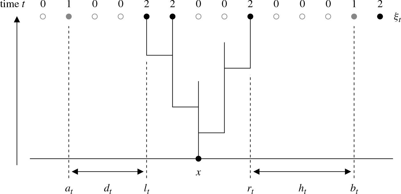
Picture related to the proof of Proposition 3.
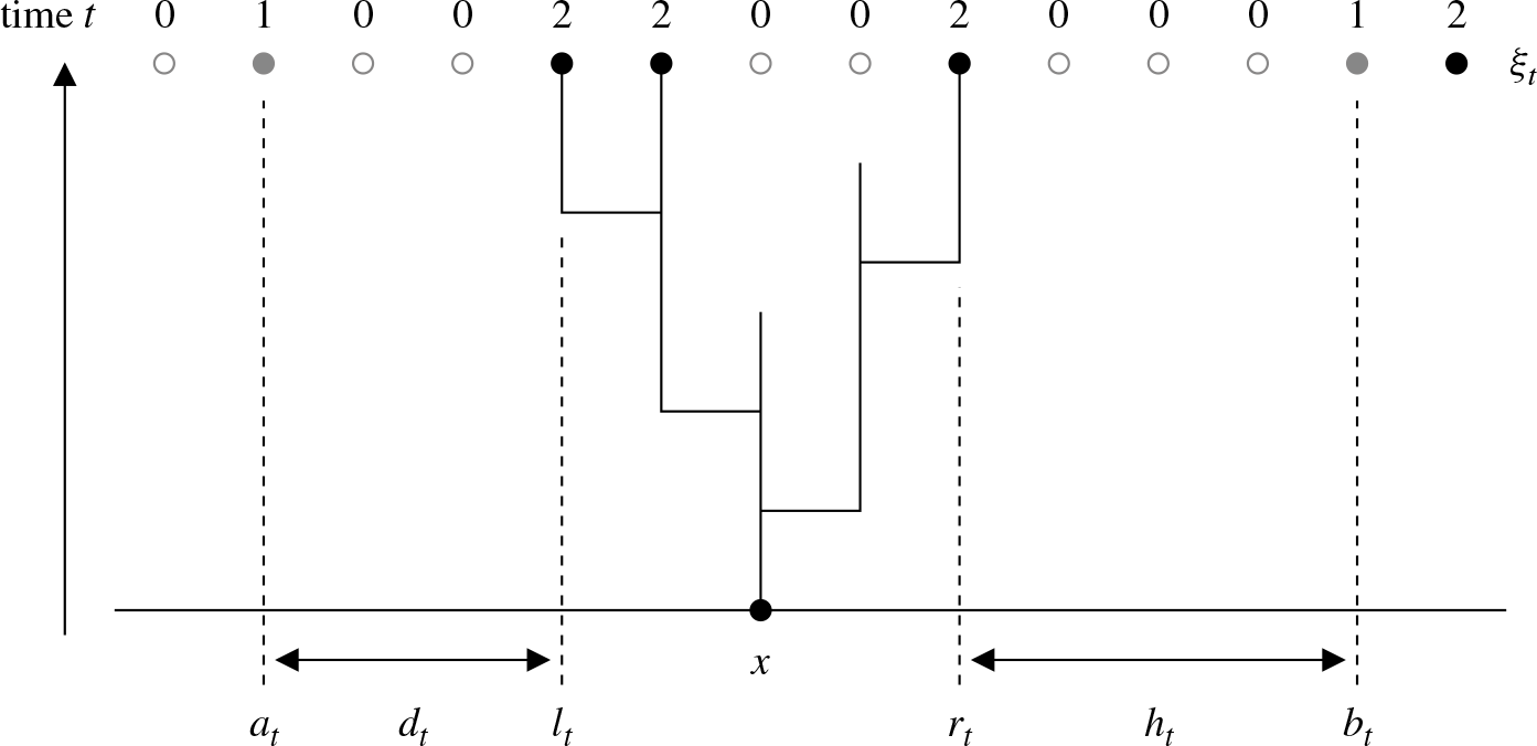
Given an interval S disjoint from  $S_1(\xi_0)$
, let
 $A_t=A_t(S)$
and let
 $\ell_t = \inf A_t$
,
 $r_t = \sup A_t$
,
 \begin{equation*} a_t = \sup \,\{x
< \ell_t \,:\, \xi_t (x) \neq 0 \} , \quad \hbox{and} \quad b_t = \inf\{x \gt r_t \,:\, \xi_t (x) \neq 0 \}. \end{equation*}
Also, let  $d_t = \ell_t - a_t$
,
 $h_t = b_t - r_t$
, and
 $m_t = \min(d_t,h_t)$
. Figure 3 gives an illustration of these quantities. Notice that, since interactions are with nearest neighbors and
 $S\cap S_1(\xi_0)=\varnothing$
by assumption, it follows that
 $[\ell_t,r_t]\cap S_1(\xi_t) = \varnothing$
for
 $t\ge 0$
, and a fortiori that
 \begin{equation}A(s,t;\,[\ell_s,r_s]) = A_t \ \hbox{for} \ s\le t.\end{equation}
Time intervals when  $m_t=1$
we call invasion, and when
 $m_t\ge 2$
we call struggle. The basic recipe for controlling
 $A_t$
is to control the duration and extent of each invasion, and to show that each struggle results, with positive probability, in the rapid and total collapse of
 $A_t$
.
We begin with struggle, which is the toughest to address; in fact, invasion will be surreptitiously taken care of in Proposition 1. In the next result we show that, starting from a fixed initial configuration  $\xi_0$
, with positive probability, collapse of
 $A_t$
occurs before invasion, uniformly over finite intervals S and
 $\xi_0$
such that
 $S_1(\xi_0)$
is disjoint from S. In addition, we show that if collapse occurs, then it is exponentially fast. This makes use of the comparison property (13) as well as the asymmetry (12), and the fact that in the absence of invasion (that is, when
 $m_t>1$
) the particles in
 $A_t$
do not interact with the particles outside
 $A_t$
. Using these estimates and an iterative restarting argument, we can then prove Proposition 1, which then easily leads to Propositions 2 and 3, at which point we have enough to tackle the proof of (10) and (11). In the following proofs, c and C are strictly positive constants such that the given statements hold for c and all smaller values than c, or C and all larger values than C, which will mean that
 $c, 1/C$
are allowed to decrease from step to step.
Lemma 1. There are  $p,c,C \gt 0$
such that, if
 $S\subset {\mathbb{Z}}$
is a finite interval,
 $S \cap S_1(\xi_0) = \varnothing$
, and
 $m_0\ge 2$
, then letting
 $\tau=\inf\{t\colon m_t=1\}$
,
 ${\rm P}(\tau = \infty) \ge p$
and, for
 $t>0$
,
 \begin{equation*}\max({\rm P}(r_s \gt r_0 - \e^{cs} \ \hbox{for some} \ s \gt t \ \hbox{and} \ \tau = \infty), \ {\rm P}(t \lt \tau
< \infty) )\leq C \,\e^{-ct}.\end{equation*}
Proof. Using a pair of independent substructures that we denote  $\Omega_1,\Omega_2$
, define generalized stacked contact processes
 $\zeta_t^{1-}, \zeta_t^{1+}$
and
 $\zeta_t^2$
with the same parameters as
 $\xi_t$
and with initial configurations
 \begin{align*} \zeta_0^{1-} (x) &= {\mathbf{1}}(\xi_0(x) \ne 0, x
< \min S), \quad \zeta_0^{1+}(x) = {\mathbf{1}}(\xi_0(x) \ne 0, x \gt \max S) \quad \text{and} \ \\ \\[-5pt] \zeta_0^2 (x) &= 2 \,{\mathbf{1}} (\xi_0(x)=2, \ x \in S ). \end{align*}
Define  $\zeta_t^1$
by
 $\zeta_t^1(x) = \max(\zeta_t^{1-}(x),\zeta_t^{1+}(x))$
, noting
 $\zeta_t^1$
is a stacked contact process with initial configuration
 ${\mathbf{1}}(\xi_0(x) \ne 0, x \notin S)$
, independent of
 $\zeta_t^2$
. For all t,
 $\zeta_t^1$
has no sites of type 2, and since
 $\delta=0$
,
 $\zeta_t^2$
has no sites of type 1. Let
 \begin{equation*}\begin{array}{r@{\,}c@{\,}l@{\quad}r@{\,}c@{\,}l} \ell_t^{\prime} &=& \inf\{y\,:\,\zeta_t^2(y) \ne 0\}, & r_t^{\prime} &=& \sup\{y\,:\,\zeta_t^2(y) \ne 0\} , \quad\hbox{and}\\ \\[-5pt] a_t^{\prime} &=& \sup\{y\,:\,\zeta_t^{1-}(y) \ne 0\}, & b_t^{\prime} &=& \inf\{y\,{:}\,\zeta_t^{1+}(y) \ne 0\}.\end{array}\end{equation*}
Let  $d_t^{\prime} = \ell_t^{\prime}-a_t^{\prime}$
,
 $h_t^{\prime} = b_t^{\prime}-r_t^{\prime}$
, and
 $m_t^{\prime}=\min(d_t^{\prime},h_t^{\prime})$
.
Since  $A_t(S)$
and
 $A_t({\mathbb{Z}} \setminus S)$
are separated (have no adjacent sites) for
 $t<\tau$
, we can define
 $\xi_t$
as follows. For
 $t<\tau$
, use
 $\Omega_2$
and the initial configuration
 $\xi_0\, {\mathbf{1}}(S)$
to determine
 $\xi_t(x)$
for
 $x\in A_t(S)$
and use
 $\Omega_1$
and the initial configuration
 $\xi_0\,{\mathbf{1}}({\mathbb{Z}}\setminus S)$
to determine
 $\xi_t(x)$
for
 $x\notin A_t(S)$
. Then use
 $\xi_\tau$
and
 $\Omega_1$
to determine
 $\xi_t$
for
 $t\ge \tau$
. This furnishes a coupling of
 $\xi_t$
with
 $\zeta_t^{1-},\zeta_t^{1+},\zeta_t^2$
, and this coupling has the property that, for all
 $t \le \tau$
,
 \begin{equation*}A_t(S) = \{x \,:\, \zeta_t^2 (x) = 1 \}\quad \hbox{and} \quad A_t({\mathbb{Z}} \setminus S) \subseteq \{x \,:\, \zeta_t^1 (x) = 1 \} .\end{equation*}
The first statement is clear, while the second statement follows from (13). It follows in particular that  $a_t \le a_t^{\prime}$
,
 $\ell_t \ge \ell_t^{\prime}$
,
 $r_t \le r_t^{\prime}$
, and
 $b_t \ge b_t^{\prime}$
, and thus
 $d_t \ge d_t^{\prime}$
,
 $h_t \ge h_t^{\prime}$
, and
 $m_t \ge m_t^{\prime}$
for
 $t\le \tau$
. To simplify matters we note that
 $\tau = \tau_{\ell} \wedge \tau_r$
, where
 \begin{equation*}\tau_\ell = \inf\{t\,:\,d_t=1\} \quad \hbox{and} \quad \tau_r = \inf\{t\,:\,h_t=1\}.\end{equation*}
In the estimates that follow, c, C, and D are positive constants and  $c, 1/C$
may get smaller from step to step. By the monotonicity of the contact process, the set of occupied sites
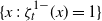 $\{x \,:\, \zeta_t^{1-} (x) = 1 \}$
of
 $\zeta_t^{1-}$
is dominated by the pure birth process in which particles do not die and give birth onto neighboring sites at rate
 $\lambda_{10}$
, similarly for
 $\zeta_t^{1+}$
, and for
 $\zeta_t^2$
with
 $\lambda_{20}$
instead of
 $\lambda_{10}$
. In particular,
 \begin{equation*} {\rm P} (b_t^{\prime} - r_t^{\prime} \lt n) \leq {\rm P} (h_0 - \mathrm{Poisson} \, ((\lambda_{10} + \lambda_{20}) \,t)
< n) \qquad \hbox{for all } n \gt 0, \end{equation*}
and, applying a standard large deviations estimate, we get
 \begin{equation} {\rm P} (h_s^{\prime}
< 2 \ \hbox{for some} \ s \leq h_0 / (2 \,(\lambda_{10} + \lambda_{20}))) \leq C \,\e^{-ch_0}.\end{equation}
Also, for each  $t \gt 0$
,
 \begin{equation} {\rm P} (b_s^{\prime}
< b_0 - 2 \lambda_{10} \,t \ \hbox{for some} \ s \leq t) \leq \e^{-ct}.\end{equation}
To control  $r_s^{\prime}$
, we use a known estimate at integer times, then a Poisson estimate at in-between times.
From (12) and the assumption  $\lambda_{20} \lt \lambda_c$
, for
 $t>0$
,
 \begin{equation} {\rm P} (r_t^{\prime} \gt r_0 - e^{ct}) \leq C \,\e^{-ct}.\end{equation}
In addition, since the displacement in one unit of time is dominated by a Poisson random variable with parameter  $\lambda_{20}$
, for any integer
 $k \geq 0$
we have
 \begin{equation} {\rm P} (r_s^{\prime} - r_n^{\prime} \gt k \ \hbox{for some} \ s \in [n, n + 1]) \leq C \,\e^{-ck}.\end{equation}
Combining (17) with  $t=n$
and (18), we deduce that
 \begin{equation} {\rm P} (r_s^{\prime} \gt r_0 - \e^{cn} + n \ \hbox{for some} \ s \in [n, n + 1]) \leq C \,\e^{-cn} .\end{equation}
Then, combining with (16) evaluated at  $t = n + 1$
, for each integer
 $n \geq 1$
,
 \begin{equation} {\rm P} (h_s^{\prime}
< h_0 + \e^{cn} - (1 + 2 \,\lambda_{10})(n + 1) \ \hbox{for some} \ s \in [n, n + 1]) \leq C \,\e^{-cn}. \end{equation}
To deduce the first estimate we distinguish two cases, where  $D>0$
is a large enough constant.
Case 1: $m_0 \gt D$
For one side of the argument,
 $h_0 \gt D$
suffices; an analogous argument applies to the other side assuming
 $d_0>D$
. The bound on
 $h_s^{\prime}$
in (20) is at least two for all n. Recalling that
 $h_t \ge h_t^{\prime}$
for
 $t\le\tau$
, then combining (15) with (20) summed over
 $n \geq \lfloor h_0 / (2 \,(\lambda_{10} + \lambda_{20})) \rfloor$
,
 \begin{equation} \begin{array}{r@{\quad}c@{\quad}l} {\rm P}(\tau_r
< \infty) &=& {\rm P}(\inf_{t \ge 0}h_t \le 1) \le {\rm P} (\inf_{t \ge 0}h_t^{\prime} \le 1) \\ \\[-5pt] & \leq & C\e^{-ch_0} + \sum_{n \geq ch_0} \,C \,\e^{-cn} \leq C \,\e^{-ch_0} \qquad \hbox{when } h_0 \gt D, \end{array}\end{equation}
where c, C do not depend on D. By reflection invariance, the same holds for  $\tau_\ell$
. If D is large enough that
 $C\e^{-cD}<1/2$
we find that
 ${\rm P}(\tau = \infty) \ge 1-2C\e^{-cD} = {\varepsilon}$
for some
 ${\varepsilon}>0$
.
Case 2: $m_0 \le D$
Given S, let E denote the event where, in one unit of time, there is a death at every site in
 $[\inf S-D,\inf S-1]\cup [\sup S+1,\sup S+D]$
and no birth onto any vertex in the same set. Since the birth rate onto any vertex is at most
 $2{\lambda}_{10}$
and the death rate at any site is 1,
 \begin{equation*}{\rm P}(E) \ge (1-\e^{-1})^{4D}(\e^{-2{\lambda}_{10}})^{4D} = \delta>0,\end{equation*}
with  $\delta$
depending on D but not on S. Note that on E,
 $\tau>1$
and
 $m_1>D$
. Using the Markov property and the previous result,
 \begin{equation*}{\rm P}(\tau=\infty) \ge {\rm P}(\tau>1 \ \hbox{and} \ m_1 \gt D){\rm P}(\tau=\infty \mid \tau>1 \ \hbox{and} \ m_1>D) \ge \delta {\varepsilon},\end{equation*}
which gives the first statement with  $p=\delta{\varepsilon}>0$
.
Now, in (19) above, for  $n \geq n_0$
for some
 $n_0$
, absorb n into
 $-\e^{cn}$
by decreasing c, then increase C to account for
 $n \lt n_0$
. Then, for any
 $t \gt 0$
, summing (19) over
 $n \geq \lfloor t \rfloor$
,
 \begin{equation*} {\rm P} (r_s^{\prime} \gt r_0^{\prime} - \e^{-cs} \ \hbox{for some} \ s \gt t) \leq C \,\e^{-ct}.\end{equation*}
On the event  $\{\tau = \infty \}$
, we have
 $r_t \le r_t^{\prime}$
for all
 $t \geq 0$
, and the second statement follows. Using the two bounds (16) and (17) above, and noting that
 $m_0\ge 2$
,
 \begin{equation*} {\rm P} (h_t^{\prime}
< 2 + \e^{ct} - 2 \,\lambda_{10} \,t) \leq C \,\e^{-ct} \end{equation*}
and for t large enough,  $2 + \e^{ct} - 2 \, \lambda_{10} \, t \ge t$
. Since
 $h_t \ge h_t^{\prime}$
for
 $t\le \tau$
, it follows that
 \begin{equation*} {\rm P}( h_t \lt t, \ t<\tau) \le C \e^{-ct},\end{equation*}
and an analogous estimate applies to  $d_t$
. For t large enough, using the above and (21),
 \begin{equation*} \begin{array}{r@{\,}c@{\,}l} {\rm P} (t \lt \tau \lt \infty) & = & {\rm P}(m_t \lt t, \ t<\tau<\infty) + {\rm P}(m_t \ge t, \ t<\tau<\infty) \\ \\[-5pt] &\le& {\rm P}(m_t \lt t, \ t<\tau) + {\rm P}(t<\tau<\infty \mid m_t \ge t)\\ \\[-5pt] &\le& {\rm P}(h_t \lt t, \ t<\tau) + {\rm P}(d_t<t, \ t<\tau) \\ \\[-5pt] &+& {\rm P}(t<\tau_r<\infty \mid m_t \ge t) + {\rm P}(t<\tau_\ell<\infty \mid m_t \ge t)\\ \\[-5pt] &\le& 4C \e^{-ct}. \end{array} \end{equation*}
This completes the proof.
Lemma 2. Let  $T=\inf\{t\,:\,m_t \ge 2\}$
. There are positive constants c,c such that, if
 $S\subset {\mathbb{Z}}$
is a finite interval and
 $S\cap S_1(\xi_0)=\varnothing$
, then
 \begin{equation*}{\rm P}( T >t) \le C\e^{-ct}.\end{equation*}
Proof. Let  $s_0=0$
and
 $s_1,s_2,\dots$
denote the times when either death occurs at
 $\ell_t-1$
or
 $r_t+1$
, or infection occurs across either the edge
 $(\ell_t,\ell_t-1)$
or
 $(r_t,r_t+1)$
. Then
 $T \le s_{2K}$
where
 \begin{equation*}K = \inf\{k\,:\, \hbox{death occurs at } (\ell_t-1,s_{2k-1}) \hbox{ and } (r_t+1,s_{2k})\}.\end{equation*}
Clearly,  $K \preceq \mathrm{Geometric \,}((1/2{\lambda}_{21})^2)$
and
 $\{s_{k+1}-s_k \colon k\ge 0\} \preceq \{\sigma_k \colon k\ge 0\}$
, an independent and identically distributed sequence of
 $\exp(2)$
random variables. A routine estimate gives the result.
Next, we show the position of the rightmost pathogen in any  $A_t$
goes to
 $- \infty$
exponentially fast. This is the analog of the second estimate in Lemma 1 but dropping the condition
 $\tau=\infty$
. This result is then used in the subsequent lemma to show that the probability that the rightmost pathogen moves n steps to the right of its initial position decays exponentially with n.
Proposition 1. There are positive constants c,C such that, if  $S\subset {\mathbb{Z}}$
is a finite interval and
 $S\cap S_1(\xi_0)=\varnothing$
, then
 \begin{equation*} {\rm P}(r_t \gt r_0 - \e^{ct}) \leq C \,\e^{-ct}. \end{equation*}
Proof. Define recursively the two sequences of stopping times  $(\tau_i)_{i\ge 0}$
and
 $(T_i)_{i\ge 0}$
by
 $\tau_0=0$
,
 $T_0 = \inf\{t \ge 0\,{:}\,m_t=2\}$
, and, recursively for
 $i\ge 1$
,
 \begin{equation*}\begin{array}{r@{\,\,}c@{\,\,}l}\tau_i &=& \inf \,\{t \gt T_{i-1} \,:\, m_t = 1 \}, \\ \\[-5pt] T_i &=& \inf \,\{t \gt \tau_i \,:\, m_t = 2 \},\end{array}\end{equation*}
with the convention  $\inf \varnothing = \infty$
. Let
 $N = \inf\{i\,{:}\,\tau_i=\infty\}$
. Recursively at each time
 $\tau_i$
, applying the strong Markov property and noting (14), then applying the first result of Lemma 1 with
 $S = [\ell_{\tau_i},r_{\tau_i}]$
we find that
 \begin{equation*} N \preceq - 1 + \mathrm{Geometric \,} (p) , \end{equation*}
where  $\preceq$
means stochastically smaller. Doing the same, but applying the third result of Lemma 1,
 \begin{equation*}\{(\tau_i - T_{i-1}) \,{\mathbf{1}}(N \geq i) \colon i>0\} \preceq \{\sigma_i \,{\mathbf{1}} (N \geq i ) \colon i>0\},\end{equation*}
where  $\sigma_1,\sigma_2,\ldots$
is a sequence of independent, identically distributed random variables independent of the random variable N and such that
 \begin{equation*} {\rm P} (\sigma_i \gt t) = \min \,(C \e^{-ct}, 1) \qquad \hbox{for all } t \gt 0. \end{equation*}
Using Lemma 2, the same holds for  $\{(T_i-T_{i-1}) {\mathbf{1}} (N \ge i) \colon i>0\}$
. Letting
 $n = \lceil t /4 {\rm E} [\sigma_i]\rceil$
, and applying a large deviations bound,
 \begin{equation}\begin{array}{r@{\,}c@{\,}l} {\rm P} (\tau_N \gt t) &\le& {\rm P}((\tau_N-T_{N-1}) + \cdots + (\tau_1 - T_0) \gt t/2) \\ \\[-5pt] &&+\ {\rm P}((T_{N-1}-\tau_{N-1}) + \cdots + (T_0 - \tau_0) \gt t/2)\\ \\[-5pt] & \leq & 2{\rm P} (\sigma_1 + \cdots + \sigma_N \gt t/2) \\ \\[-5pt] & \leq & 2{\rm P} (N \gt n) + 2{\rm P} (\sigma_1 + \cdots + \sigma_n \gt 2 n \,{\rm E} [\sigma_i]) \leq 2C \,\e^{-cn} \leq 2C \,\e^{-ct}. \end{array} \end{equation}
We may assume that  $\lambda_{20} \leq \lambda_{21}$
, since otherwise
 $A_t$
is dominated by a contact process with infection rate
 $\lambda_{20}<\lambda_c$
and initial sites S, and the result then follows directly from (12). Comparing the set of sites in state 2 to a pure birth process with no deaths and with birth to adjacent sites at rate
 $\lambda_{21}$
, a large deviations estimate gives
 $c, C \gt 0$
such that
 \begin{equation} {\rm P} (r_t \gt r_0 + 2 \,\lambda_{21} \,t) \leq C \,\e^{-ct} \qquad \hbox{for all } t \gt 0.\end{equation}
For any  $c \gt 0$
, there is
 $t_0$
such that
 $\lambda_{21} \,t \lt \e^{ct} - \e^{ct/2}$
for all
 $t \gt t_0$
, in which case
 \begin{equation} \begin{array}{r@{\,}c@{\,}l} {\rm P} (r_t \gt r_0 - \e^{ct/2}) & \leq & {\rm P} (r_{t/2} \gt r_0 + \lambda_{21} \,t) \\ \\[-5pt] & & \hspace*{10pt} + \ {\rm P} (r_t \gt r_0 - \e^{ct/2} \ \hbox{and} \ r_{t/2} \leq r_0 + \lambda_{21} \,t) \\ \\[-5pt] & \leq & {\rm P} (r_{t/2} \gt r_0 + \lambda_{21} \,t) + {\rm P} (r_t \gt r_{t/2} - \lambda_{21} \,t - \e^{ct/2}) \\ \\[-5pt] & \leq & {\rm P} (r_{t/2} \gt r_0 + \lambda_{21} \,t) + {\rm P} (r_t \gt r_{t/2} - \e^{ct}) \end{array}\end{equation}
for all  $t \gt t_0$
. On the other hand,
 \begin{equation} {\rm P} (r_t \gt r_{t/2} - \e^{ct}) \le {\rm P} (\tau_N \gt t/2) + {\rm P}(r_t \gt r_{t/2}- \e^{ct}, \ \tau_N \le t/2) .\end{equation}
Letting  $\tau(t) = \inf\{s>t\,:\,m_s=1\}$
, the event
 $\tau_N \le t/2$
is equivalent to
 $\tau(t/2)=\infty$
. Applying the second result of Lemma 1 with
 $S=[\ell_{t/2},r_{t/2}]$
we find that
 \begin{equation*}{\rm P}(r_t \gt r_{t/2} - \e^{ct} \ \hbox{and} \ \tau(t/2)=\infty) \le C\e^{-ct}.\end{equation*}
Combining with (22)–(25) gives the desired estimate when  $t \gt t_0$
. If
 $t\leq t_0$
then, after increasing C if necessary, the estimate holds for all values of t.
Proposition 2. There is  $C \gt 0$
such that, if
 $S\subset {\mathbb{Z}}$
is a finite interval and
 $S \cap S_1(\xi_0) = \varnothing$
, then
 \begin{equation*} {\rm P} (r_t \gt r_0 + n \ \hbox{for some} \ t \geq 0) \leq C \,\e^{-cn}.\end{equation*}
Proof. Comparing to a pure birth process as above,
 \begin{equation*} {\rm P} (r_s \gt r_0 + n \ \hbox{for some} \ s \leq m_0) \leq C \,\e^{-cn} \quad \hbox{for} \quad m_0 = \lfloor n / 2 \lambda_{21} \rfloor. \end{equation*}
If  $n \ge n_0 = \sup_{m\ge 0}- \e^{cm} + m$
, then using Proposition 3 and large deviations for the Poisson distribution with parameter
 $\lambda_{21}$
,
 \begin{equation*} \begin{array}{l} {\rm P} (r_s \gt r_0 + n \ \hbox{for some} \ s \in [m, m + 1]) \\ \\[-5pt] \hspace*{18pt} \leq \ {\rm P} (r_m \gt r_0 - \e^{-cm}) + {\rm P} (r_s \gt r_m + m \ \hbox{for some} \ s \in [m, m + 1]) \leq C \,\e^{-cm}. \end{array} \end{equation*}
Summing over  $m \geq m_0$
gives the desired estimate for
 $n\ge n_0$
; for
 $n<n_0$
increase C if necessary.
We can now show that the set of descendants is exponentially bounded in both space and time.
Proposition 3. There are  $c, C \gt 0$
such that, if
 $x \in {\mathbb{Z}}$
and
 $\xi_0(x)=2$
,
 \begin{equation*} {\rm P}(A_t(x) \neq \varnothing) \leq C \,\e^{-ct} \quad \hbox{and} \quad {{\rm P}(A_t(x) \nsubseteq [x - n, x + n] \ \hbox{for some} \ t \geq 0) \leq C \,\e^{-cn}.} \end{equation*}
Proof. Defining  $a_t$
,
 $\ell_t$
, etc. with
 $S=\{x\}$
,
 $\ell_0=r_0=x$
, and
 $A_t(x)\ne\varnothing$
is equivalent to
 $\ell_t \le r_t$
. Using Proposition 1, reflection invariance, and a union bound,
 \begin{equation*}\begin{array}{r@{\,}c@{\,}l}{\rm P}(\ell_t \gt r_t) &\ge& {\rm P}(\ell_t \ge \ell_0 + \e^{ct} \ \hbox{and} \ r_t \le r_0-\e^{ct}) \\ \\[-5pt] &\ge & 1 - ({\rm P}(\ell_t
< \ell_0+\e^{ct}) + {\rm P}(r_t \gt r_0-\e^{ct}) \ge 1-2C\e^{-ct},\end{array}\end{equation*}
and the first result follows by taking the complement. The second result follows in the same way, except using Proposition 2.
Next, we use Proposition 3 to prove (10), which says that in an exponentially growing neighborhood of any site, eventually there are no sites in state 2. We also record an exponential estimate. Note the change in the definition of  $\ell_t^x,r_t^x$
.
Proposition 4. For a site  $x \in {\mathbb{Z}}$
, let
 \begin{equation*} \ell_t^x = \sup \,\{y \leq x \,:\, \xi_t(y) = 2 \} \quad \hbox{and} \quad r_t^x = \inf \,\{y \geq x \,:\, \xi_t (y) = 2 \}. \end{equation*}
Then, there exist  $c, C \gt 0$
such that, for any
 $\xi_0$
and
 $t_0$
,
 \begin{equation*} {\rm P}(\ell_t^x \gt x - \e^{ct} \ \hbox{or} \ r_t^x
< x + \e^{ct} \ \hbox{for some} \ t \gt t_0) \leq C \,\e^{-ct_0}. \end{equation*}
Also, there exists  $c \gt 0$
such that, for any
 $\xi_0$
and any site x,
 \begin{equation*} {\rm P}(\sup \,\{t \,:\, \xi_t (y) = 2 \ \hbox{for some} \ y \ \hbox{such that} \ |y - x| \leq \e^{ct} \}
< \infty) = 1. \end{equation*}
Proof. Throughout this proof, y refers to a site which is initially in state 2. Let c, C be two constants as in Proposition 3, so that for all y,  $\xi$
, and n,
 \begin{equation*} \max({\rm P}(A_n(y) \neq \varnothing),{\rm P}(A_t(y) \nsubseteq [x-n,x+n] \ \text{for some} \ t\ge 0)) \leq C \,\e^{-cn}. \end{equation*}
Using a union bound over  $y \in [x - \e^{cn/2}, x + \e^{cn/2}]$
and that
 $A_t(y) = \varnothing$
is an absorbing property,
 \begin{equation}\begin{array}{l} {\rm P} (A_t(y) \neq \varnothing \ \hbox{for some} \ y \ \hbox{such that} \ \xi_0 (y) = 2 \\ \\[-5pt] \hspace*{80pt} \hbox{and} \ |y - x| \leq \e^{cn/2} \ \hbox{and some} \ t \geq n) \leq C \,\e^{-cn/2}. \end{array}\end{equation}
Let  $n_0$
be such that
 $n \geq n_0$
implies
 $\e^{cn/2} - \e^{c (n + 1)/4} \gt n$
. If
 $|y - x| = \lceil \e^{cn/2} \rceil + m$
for integer
 $m \geq 0$
and any
 $n \geq n_0$
, then, using the second half of Proposition 3,
 \begin{equation*} {\rm P} (\inf_t \min \{|z-x| \colon z \in A_t(y)\} \leq \e^{c (n + 1)/4}) \leq C \,\e^{-c (n + m)}. \end{equation*}
Taking C larger if necessary makes the previous inequality also true for all  $n \lt n_0$
. Then, taking a union bound and increasing C at the last step gives
 \begin{equation} \begin{array}{l} {\rm P} (\inf_t \min \{|z-x|\colon z \in A_t(y)\} \leq \e^{c (n + 1)/4} \ \hbox{for some} \ y \\ \\[-5pt] \hspace*{50pt} \hbox{such that} \ |y - x| \gt \e^{cn/2} \ \hbox{and} \ \xi_0 (y) = 2) \leq {C (1 - \e^{-c}) \,\e^{-cn} \leq C \,\e^{-cn}}. \end{array} \end{equation}
 \begin{equation*} {\rm P} (\xi_t (y) = 2 \ \hbox{for some} \ y \in [x - \e^{ct/4}, x + \e^{ct/4}] \ \hbox{and} \ t \in [n, n + 1]) \leq C \,\e^{-cn/2}. \end{equation*}
Given  $t_0$
, summing over
 $n \geq \lfloor t_0 \rfloor$
gives the first statement. Summing over all n and using the Borel–Cantelli lemma finishes the proof.
In what follows, a mark refers to a Poisson point in the graphical representation. Marks are named by their effect on the target site, so, for example, a  $0 \to 1$
mark is an edge mark at some time t along a directed edge (x, y) such that if
 $\xi_{t^-} (x) = 1$
and
 $\xi_{t^-} (y) = 0$
then
 $\xi_t (y) = 1$
. Also, a death mark refers to a
 $\star \to 0$
event, while a birth mark is a
 $0 \to \star$
event, where
 $\star \neq 0$
. Note that since the graphical representation consists of at most a countably infinite number of Poisson point processes, with probability one, no two marks occur at the same time.
Next, we use Proposition 4 to produce an interval that grows linearly in time and is devoid of pathogens.
Lemma 3. For any  $\mu \gt 0$
, there are
 $c, C \gt 0$
such that, for all integer
 $n>0$
,
 \begin{equation*} {\rm P} (\xi_t (x) = 2 \ \hbox{for some} \ |x| \leq n / 2 + \mu t) \leq C \,\e^{-cn} \end{equation*}
for all  $\xi_0$
such that
 $\xi_0(x) \neq 2$
for all
 $|x| \leq n$
.
Proof. Let  $y = n + m$
with
 $m \gt 0$
; a similar argument applies to
 $-y$
. Using Proposition 3 gives the existence of constants
 $c, C \gt 0$
such that, for all
 ${\varepsilon} \gt 0$
,
 \begin{equation*} \begin{array}{l} {\rm P} (A_{{\varepsilon} y}^y \neq \varnothing \ \hbox{or} \ \inf_t A_t^y
< 2y/3) \leq C \,\e^{-c {\varepsilon} y}. \end{array} \end{equation*}
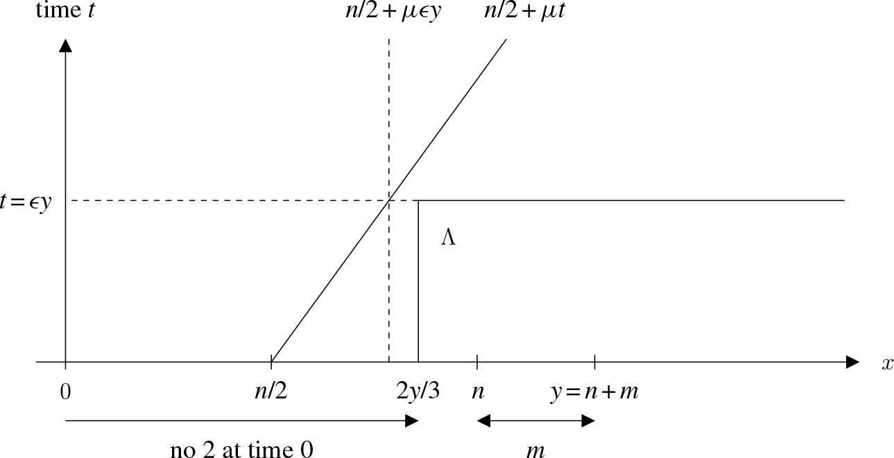
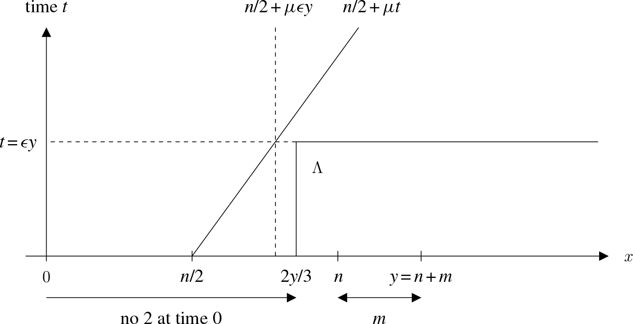
On the complement of the above event, the descendants of (y, 0) are contained in
 \begin{equation*} \Lambda \,:\!= \{(x, t) \,:\, x \geq 2y/3 \ \hbox{and} \ 0 \leq t \leq {\varepsilon} y \}. \end{equation*}
A quick sketch (see Figure 4) shows that the rectangle  $\Lambda$
is disjoint from the set
 \begin{equation*} \{(x, t) \,:\, t \geq 0 \ \hbox{and} \ |x| \leq n / 2 + \mu t \} \end{equation*}
provided the top left corner of  $\Lambda$
lies to the right of the line
 $x = n / 2 + \mu t$
, which is the condition
 \begin{equation*} n / 2 + \mu {\varepsilon} y
< 2y / 3. \end{equation*}
Since  $n \leq y$
, this condition is satisfied if
 ${\varepsilon} \lt 1/ 6 \mu$
. Summing over
 $m \gt 0$
for both
 $y = n + m$
and
 $y = - n - m$
then gives the desired result.
Picture related to the proof of Lemma 3.
A related notion to the descendants is the cluster, that we need only define for type 1, as follows. Suppose  $\xi_s (x) = \xi_t (y) = 1$
for some x, y and
 $s \leq t$
. Then, we say that (y, t) belongs to the cluster of (x, s) if there are times and sites
 \begin{equation*} s = t_0 \lt t_1 \lt \cdots
< t_{k - 1} \leq t_k = t \quad \hbox{and} \quad x = x_1, x_2, \ldots, x_k = y \end{equation*}
such that the following two conditions hold:
• For
$j = 1, 2, \ldots, k$
, we have
$\xi_r (x_j) = 1$
for all times
$r \in [t_{j - 1}, t_j]$
.• For
$j = 1, 2, \ldots, k - 1$
, there is a
$0 \to 1$
birth mark along the edge
$(x_j, x_{j + 1})$
at time
$t_j$
.






In contrast to the definition of descendants, it is permitted to have  $\xi_{t_j^-} (x_{j + 1}) = 1$
.
If  $\xi_s (x) = 1$
then, for
 $t \geq s$
, let
 $B_t (x, s)$
denote the cluster of (x, s) at time t, that is,
 \begin{equation*} B_t (x, s) \,:\!= \{y \in {\mathbb{Z}} \,:\, (y, t) \ \hbox{is in the cluster of} \ (x, s) \}, \end{equation*}
and denote it  $B_t (x)$
for
 $s = 0$
. Again, since interactions are nearest-neighbor,
 \begin{equation*} \xi_t(y) \neq 2 \quad \hbox{for all} \quad y \in [\inf B_t (x, s), \sup B_t (x, s)] \quad \hbox{and} \quad t \geq s. \end{equation*}
As a warm-up to (11), we prove the following.
Lemma 4. Suppose  $\xi_0(0)=1$
. Let
 $\ell_t = \inf B_t (0)$
and
 $r_t = \sup B_t (0)$
, and let
 \begin{equation*} \tau = \inf \,\{t \gt 0 \,:\, \xi_t (\ell_t - 1) = 2, \ \xi_t (r_t + 1) = 2 , \ \text{or} \ B_t = \varnothing\} .\end{equation*}
Then, there are  $p, c, C \gt 0$
such that
 \begin{equation*} {\rm P}(\tau = \infty) \geq p \quad \hbox{and} \quad {\rm P} (t \lt \tau
< \infty) \leq C \,\e^{-ct} \end{equation*}
uniformly over  $\xi_0$
such that
 $\xi_0(0) = 1$
.
Proof. Define a pair of independent copies  $\xi_t^1$
and
 $\xi_t^2$
of the generalized stacked contact process with initial configurations
 \begin{equation*} \xi_0^1 (y) = \xi_0 (y) \,{\mathbf{1}} \{y = 0 \} \quad \hbox{and} \quad \xi_0^2 (y) = \xi_0 (y) \,{\mathbf{1}} \{y \neq 0 \}. \end{equation*}
Also define
 \begin{equation*} \begin{array}{r@{\quad}c@{\quad}l} \ell_t^1 = \inf \,\{x \,:\, \xi_t^1 (x) = 1 \} & \hbox{and} & r_t^1 = \sup \,\{x \,:\, \xi_t^1 (x) = 1 \} , \\ \\[-5pt] a_t^2 = \sup \,\{x
< \ell_t^1 \,:\, \xi_t^2 (x) = 2 \} & \hbox{and} & b_t^2 = \inf \,\{x \gt r_t^1 \,:\, \xi_t^2 (x) = 2 \} , \end{array} \end{equation*}
so that  $\tau$
can also be expressed as
 \begin{equation*} \tau = \inf \,\{t \gt 0 \,:\, \ell_t^1 - a_t^2 \leq 1, \ b_t^2 - r_t^1 \leq 1 , \ \text{or} \ \xi_t^1 \equiv 0\}. \end{equation*}
To show that  $\tau = \infty$
with positive probability, first we fix n and consider the case
 $\min (|a_0^2|, |b_0^2|) \geq n$
. Using large deviations estimates for the Poisson distribution, we can show that
 \begin{equation*} {\rm P} (\max (|\ell_t^1|, |r_t^1|) \geq 2 \lambda_{10} \,t + n / 2 - 1 \ \hbox{for some} \ t \gt 0) \leq C \,\e^{-cn}. \end{equation*}
To do so, it suffices to first make an estimate for  $t \leq m_0 \,:\!= \lfloor n / 4 \lambda_{10} \rfloor$
, then for
 $t \in [m, m + 1]$
for each
 $m \geq m_0$
, then to take a union bound. Then, taking
 $\mu = 2 \lambda_{10}$
and using Lemma 3, for integer
 $n>0$
we have
 \begin{equation*} {\rm P} (\min (|a_t^2|, |b_t^2|) \leq 2 \lambda_{10} \,t + n/2 \ \hbox{for some} \ t \gt 0) \leq C \,\e^{-cn}. \end{equation*}
Since  $\lambda_{10}>\lambda_c$
by assumption,
 $q\,:\!={\rm P}(\xi_t^1 \not\equiv 0 \ \text{for all } t)>0$
. Moreover, if
 $\xi_t^1 \not\equiv 0 \ \text{for all } t$
and
 $\min \,(|a_t^2|, |b_t^2|) \gt \max (|\ell_t^1|, |r_t^1|) \ \hbox{for all} \ t \gt 0$
then
 $\tau=\infty$
, so taking n large enough that
 $2C\e^{-cn}<q/2$
, we find that if
 $\xi (x) \neq 2$
for
 $|x| \leq n$
then
 \begin{equation*} {\rm P} (\tau = \infty) \geq q-q/2 = q/2. \end{equation*}
For  $\xi$
such that
 $\xi (0) = 1$
, the probability
 \begin{equation*} {\rm P} (\xi_1 (0) = 1 \ \hbox{and} \ \xi_1 (x) = 0 \ \hbox{for all} \ 0
< |x| \leq n) \end{equation*}
is at least the probability that, on the time interval [0, 1], there are no birth marks along edges touching  $[\!-n, n]$
, there is no death mark at 0, and there is a death mark at every x with
 $0 \lt |x| \leq n$
, and this probability is at least
 $2p/q$
for some
 $p \gt 0$
. Using the Markov property and the estimate on
 $\tau = \infty$
in the previous case then gives
 ${\rm P} (\tau = \infty) \geq (2p/q)(q/2)=p \gt 0$
as desired.
To deduce the estimate on  ${\rm P} (t \lt \tau \lt \infty)$
, we note that
 \begin{equation*} {\rm P} (\max (|\ell_s^1|, |r_s^1|) \geq 2 \lambda_{10} \,s \ \hbox{for some} \ s \geq t) \leq C \,\e^{-ct}, \end{equation*}
which can be proved by applying an estimate at each integer time  $n \gt t$
and summing over n. Then, combining with the first statement in Proposition 3 and noting that
 \begin{equation*} t \lt \tau
< \infty \quad \hbox{implies that} \quad \max (|\ell_s^1|, |r_s^1|) \geq \min (|a_s^2|, |b_s^2|) - 1 \ \hbox{for some} \ s \gt t, \end{equation*}
we deduce the estimate on  ${\rm P} (t \lt \tau \lt \infty)$
.
We are now ready to establish (11), which states the existence of a linearly growing region starting from a random space-time point in which the process agrees with the contact process with parameter  $\lambda_{10}$
. This will also complete the proof of Theorem 2.
Proof of (11). Given (x, s), for  $t \geq s$
recall that
 $B_t (x, s)$
denotes the cluster of (x, s) at time t. Let
 $\tau_0 = 0$
, and
 $x_0$
be any site with
 $\xi (x_0) = 1$
. Without loss of generality, suppose that the set
 $\{x \gt 0 \,:\, \xi (x) = 1 \}$
is infinite, and define
 $x_i$
and
 $\tau_i$
recursively for
 $\lambda_{21} \lt \infty$
by letting
 \begin{equation*} \begin{array}{r@{\,}c@{\,}l} \ell_t^i & = & \inf \,B_t (x_i, \tau_i) , \\ \\[-5pt] r_t^i & = & \sup \,B_t (x_i, \tau_i) , \\ \\[-5pt] \tau_{i + 1} & = & \inf \,\{t \gt \tau_i \,:\, \xi_t (\ell_t^i - 1) = 2 \ \hbox{or} \ \xi_t (r_t^i + 1) = 2 \} , \\ \\[-5pt] x_{i + 1} & = & \inf \,\{x \gt x_i \,:\, \xi_{\tau_{i + 1}} (x) = 1 \}, \end{array} \end{equation*}
with the value of  $x_i$
being unimportant if
 $\tau_i = \infty$
. Note that if time
 $\tau_i \lt \infty$
then site
 $x_{i + 1}$
is well defined due to the fact that
 \begin{equation*} \{\xi \,:\, \xi (x) = 1 \ \hbox{for infinitely many} \ x \gt 0 \} \end{equation*}
is an invariant set for the dynamics. Let  $N = \sup \,\{i \,:\, \tau_i \lt \infty \}$
. Applying the strong Markov property and using Lemma 4, we obtain that N is at most geometric with parameter p. In addition, by the second part of Lemma 4, for
 $i = 0, 1, 2, \ldots$
,
 \begin{equation*} \tau_{i + 1} - \tau_i \preceq T_i \quad \hbox{where} \quad {\rm P} (T_i \gt t) \leq \max \,(1, C \e^{-ct}) \end{equation*}
and the random variables  $T_i$
are independent. In particular,
 $\tau_N$
is almost surely finite. Let
 $T = \tau_N$
,
 $X = x_N$
,
 $\ell_t = \ell_t^N$
, and
 $r_t = r_t^N$
.
Recall that  $\zeta_t$
denotes the process with initial configuration
 $\zeta_0 (x) = 1$
for all x. Since
 $\lambda_{10} \gt \lambda_{20}$
by assumption, a straightforward coupling argument shows that, for any configuration
 $\xi_0$
,
 \begin{equation*} \{x \in {\mathbb{Z}} \,:\, \xi_t (x) \neq 0 \} \subseteq \{x \in {\mathbb{Z}} \,:\, \zeta (x) = 1 \}. \end{equation*}
Therefore,  $\zeta_{\tau_i} (x_i) = 1$
whenever
 $\tau_i \lt \infty$
. By definition of time
 $\tau_{i + 1}$
, the set
 $B_t(x_i,\tau_i)$
is the set of infected sites in a (single-type) contact process started from the single infected site
 $x_i$
at time
 $\tau_i$
, so a coupling found in [Reference Durrett3] shows that if
 $\tau_i \lt \infty$
then
 \begin{equation*} \xi_t (x) = \zeta_t (x) \ \hbox{for all} \ x \in [\ell_t^i, r_t^i] \ \hbox{and all} \ \tau_i \lt t
< \tau_{i + 1}. \end{equation*}
In [Reference Durrett3] it is shown that, for the contact process, on the event of single-site survival,  $-\ell_t^i/ t$
and
 $r_t^i / t \to \alpha \gt 0$
, so the same is true here provided
 $\tau_{i + 1} = \infty$
, which is the case for
 $i = N$
. The proof is now complete.
Acknowledgement
This research was supported in part by an NSERC Discovery Grant.