

1. Introduction
Structural biologists should fear for their livelihoods. As soon as the monkeys finish re-writing Hamlet, their typewriters will be upgraded to computers running Foldit (Cooper et al. Reference Cooper, Khatib, Treuille, Barbero, Lee, Beenen, Leaver-Fay, Baker, Popovic and Players2010) and a whole swathe of the scientific community will be made redundant. Come to think of it though, if the author's efforts (top score 8636, roughly equivalent to a Tetris score of 40) are anything to go by, that is not going to happen for a while … Jokes aside though, the fact that cutting-edge research has been translated into a video game (and generates interest!) stresses the aesthetic and intellectual beauty of protein structures. Another initiative from members of the Foldit group has been to run their program for structure prediction, Rosetta (Das & Baker, Reference Das and Baker2008), on BOINC (http://boinc.bakerlab.org/rosetta/, http://boinc.berkeley.edu/). This immediately brings SETI (http://setiathome.berkeley.edu/) to mind, the platform of course, but mainly because it implies that proteins have the same power of popular fascination as extraterrestrial life.
Proteins govern all living systems. The structure, function, life and death of cells all rest upon structural, regulatory or defence proteins. Enzymes on the other hand catalyse the chemical reactions of an organism's metabolism. The evolution of different folds and protein families over millions of years underpins biology on a fundamental level. In terms of practical applications, the development of new drugs hinges on a better understanding of specific metabolic pathways and cellular processes encoded in protein structures.
Proteomics was revolutionised in the 1990s as mass spectrometry turned protein sequencing from a matter of days, to a matter of seconds (Wilm et al. Reference Wilm, Shevchenko, Houthaeve, Breit, Schweigerer, Fotsis and Mann1996; Steen & Mann, Reference Steen and Mann2004). This transformation has created (and continues to create) a host of new targets for structural investigation. The latest release of the RefSeq database for non-redundant protein sequences contained 10 640 515 entries (http://www.ncbi.nlm.nih.gov/refseq/, the latest release at the time of writing was dated 21 July 2010). In contrast, as of 14 September 2010, only 67 981 structures had been deposited in the PDB. The gap is not just huge but growing, as the number of known sequences doubles every 28 months (Levitt, Reference Levitt2009). While at present it is an unfeasible aim to determine all these structures experimentally, it maybe possible to map out fold space in a reasonable amount of time (Levitt, Reference Levitt2009).
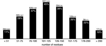
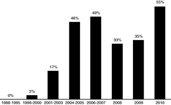
This was the aim of a number of structural proteomics initiatives set up at the turn of the century (Yokoyama et al. Reference Yokoyama, Matsuo, Hirota, Kigawa, Shirouzu, Kuroda, Kurumizaka, Kawaguchi, Ito, Shibata, Kainosho, Nishimura, Inoue and Kuramitsu2000b; Terwilliger et al. Reference Terwilliger, Stuart and Yokoyama2009). The premise being that once a relatively small fraction of structures had been solved, any number of interesting targets would be accessible via homology modelling. The main techniques used were X-ray crystallography and NMR spectroscopy. The advantages of the NMR approach are well known: proteins do not need to be crystallised, experiments are performed in a (close to) physiological environment and are sensitive to protein dynamics. On the down side, however, NMR protein structure calculation is both slow and limited to relatively small targets (see Fig. 2). The protocol established in the 1980s (Wüthrich, Reference Wüthrich1986) has survived to this day with remarkably few changes. And at the time when structural genomics projects were being set up, while robust systems for automatic data analysis were emerging (Güntert, Reference Güntert1998; Moseley & Montelione, Reference Moseley and Montelione1999), the main tasks were overwhelmingly performed manually. For a couple of centres, some of the funding was allocated specifically to NMR software development (Williamson & Craven, Reference Williamson and Craven2009). Figure 3 highlights the influence of structural proteomics, in general, on the field. (One notes in particular the plunge that corresponds to the end of the RIKEN project.) We shall see that many of the programs discussed in this review are affiliated in some way with a structural genomics centre.
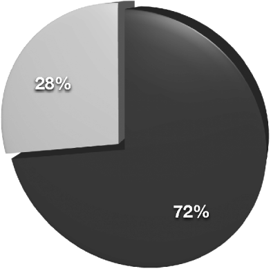
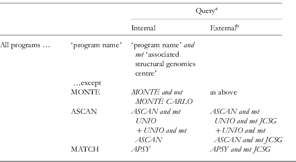
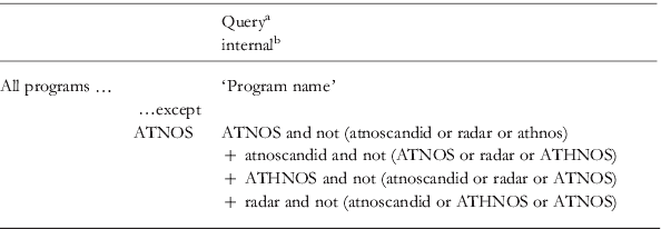
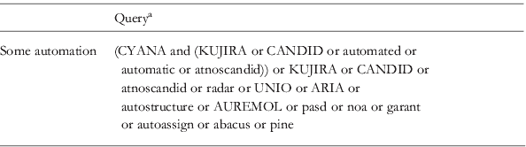
Pie-chart representation of the percentage of structures in the PDB solved using solution-state NMR with entirely manual or interactive methods (black) or with some automation (grey), as of 27 August 2010. ‘Some automation’, entails that one or more program(s) are cited that perform unsupervised NMR data analysis. Exact search strings can be found in the Appendix, Table A4.

Histograms representing, per size category (measured as the number of amino-acid residues), the percentage of solution-state NMR deposition in the PDB for which some automation was used. ‘Some automation’, entails that one or more program(s) are cited that perform unsupervised NMR data analysis. Exact search strings can be found in the Appendix, Table A5.

Histograms representing, per period, the percentage of solution-state NMR deposition in the PDB for which some automation was used. ‘Some automation’, entails that one or more program(s) are cited that perform unsupervised NMR data analysis. Exact search strings can be found in the Appendix, Table A5.

Over the past decade, technical advances in NMR hardware and experiments have also been key in the drive towards high throughput. The advent of cryo-probes in particular has lead to stunning gains in sensitivity. NMR has also benefited from ever-increasing magnetic field strengths and instrument stability. Spreading atomic connectivity pathways over several dimensions is essential in order to reduce spectral crowding and assignment ambiguity. However, such methods rely on several stages of magnetisation transfer, each reducing the sensitivity and correspondingly increasing the experimental time required to achieve an adequate signal-to-noise level. Put together, the aforesaid improvements mean for instance that multidimensional (3D+) spectra – the basis of most NMR protein structure calculations – are now routine to acquire. In parallel, a number of alternative schemes for data acquisition and processing have been developed to access even higher-dimensional correlations (Atreya & Szyperski, Reference Atreya and Szyperski2005; Malmodin & Billeter, Reference Malmodin and Billeter2005; Gryk et al. Reference Gryk, Vyas and Maciejewski2010).
It is clear that structural genomics projects have provided the main impetus for automatic NMR protein structure determination. However, interest in the matter does not end there. Crucial also are the quality and reproducibility of results. An advantage of computational approaches that is therefore just as important as their speed is their objectivity. Moreover, the availability of structure-calculation software opens the field to non-experts who may be interested in other aspects of protein science.
To date, three main approaches to automated protein structure determination have been proposed, each one based on a different NMR parameter. This review is structured likewise; we contrast the classical pathway based on the gathering of nuclear Overhauser effect (NOE) inter-proton distance constraints with more recent residual dipole coupling (RDC)- and chemical shift-based methods. The number of competing software packages is extremely disconcerting. We hope to provide a more organised view of ‘software space’ as it were, by opting for a component-by-component description of the various programs, aiming to shed light on similarities, differences, advantages and/or disadvantages where they exist.
An alternative take on the subject may be obtained from several sources, from which the evolution of the field over the past few years may be deduced (Güntert, Reference Güntert1998, Reference Güntert2003; Moseley & Montelione, Reference Moseley and Montelione1999; Gronwald & Kalbitzer, Reference Gronwald and Kalbitzer2004; Billeter et al. Reference Billeter, Wagner and Wüthrich2008; Markwick et al. Reference Markwick, Malliavin and Nilges2008). The literature on structural proteomics initiatives is vast but instructive in terms of the ambitions and limits of NMR structural biology. We found the following papers to be particularly informative (Yokoyama et al. Reference Yokoyama, Hirota, Kigawa, Yabuki, Shirouzu, Terada, Ito, Matsuo, Kuroda, Nishimura, Kyogoku, Miki, Masui and Kuramitsu2000a, Reference Yokoyama, Terwilliger, Kuramitsu, Moras and Sussman2007; Yee et al. Reference Yee, Chang, Pineda-Lucena, Wu, Semesi, Le, Ramelot, Lee, Bhattacharyya, Gutierrez, Denisov, Lee, Cort, Kozlov, Liao, Finak, Chen, Wishart, Lee, Mcintosh, Gehring, Kennedy, Edwards and Arrowsmith2002, Reference Yee, Gutmanas and Arrowsmith2006; Cyranoski, Reference Cyranoski2006; Terwilliger et al. Reference Terwilliger, Stuart and Yokoyama2009; Ledford, Reference Ledford2010). A number of reviews have newly been published, which treat the RDC (Blackledge, Reference Blackledge2005; Donald & Martin, Reference Donald and Martin2009) and chemical shift (Wishart, Reference Wishart2010) sections in more detail, NMR of proteins more generally speaking (Banci et al. Reference Banci, Bertini, Luchinat and Mori2010; Bermejo & Llinás, Reference Bermejo and Llinás2010). Finally, we only mention sample preparation techniques and new NMR experiments in the context of the automated protocol into which they have been incorporated, the reader interested in a more complete description is referred to Sundström et al. (Reference Sundström, Norin and Edwards2006), Yee et al. (Reference Yee, Gutmanas and Arrowsmith2006) and Shin & Lee (Reference Shin and Lee2008) for sample preparation and Atreya & Szyperski (Reference Atreya and Szyperski2005), Malmodin & Billeter (Reference Malmodin and Billeter2005) and Gryk et al. (Reference Gryk, Vyas and Maciejewski2010) for new experiments.
2. The classical approach
The standard approach for solving protein structures by NMR involves two stages of assignment. In the first, the chemical shifts of the NMR-active nuclei in the protein are identified according to their position in the amino-acid sequence, re-expressing the protein's primary structure in terms of an NMR-measurable parameter. In the second, a self-constrained picture of the protein fold is modelled through the evaluation of thousands of inter-proton contacts and a biophysical force field.
Magnetisation transfer through NOEs registers as signals in NOESY spectra. For two isolated protons, the NOESY peak volume is proportional to the inverse sixth power of the inter-nuclear separation. Under the isolated two-spin approximation (Cavanagh, Reference Cavanagh2007):

where C is a constant of proportionality linking the peak volume, V, to the inter-nuclear distance, d. Because of the effect of neighbouring spins, a somewhat looser relationship is assumed for proteins whereby the volume imposes an upper-distance limit on the inter-nuclear separation. Multi-spin effects, generally ignored, tend indeed to reduce the magnetisation transfer. For the same reason, the absence of an NOE signal is generally not taken as a lower-distance limit. Such conservative interpretation of the spectra relies on a dense network of upper-distance limits to reproduce the natural fold.
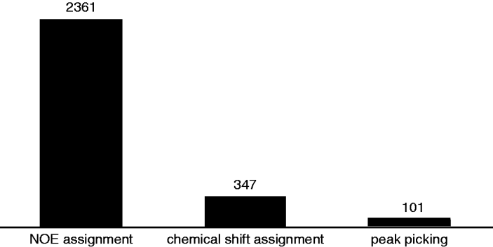
Because many of the tasks involved with this data analysis are repetitive, and involve a prodigious amount of book keeping, automation has always been a key focus. We shall cover the stages in reverse as it were, starting with NOE assignment before discussing algorithms for chemical shift assignment and peak picking. As Fig. 4 shows, this order follows how successfully the respective computer programs have established themselves in the structural biology community.
The use of automation – in terms of PDB depositions – for the different stages of the traditional protocol for NMR protein structure determination. The histograms represent the number of structures returned when searching the PDB for one of the programs published for the respective stages. Exact search strings can be found in the Appendix (Tables A1, A2 and A3).

2.1 NOE assignment
2.1.1 Chemical shift ambiguity
NOE-assignment programs start from a list of peaks (compiled from all the NMR spectra) and a list of chemical shifts, each of which corresponds to a particular atom (or group of atoms) in the protein. It is common for the chemical shifts of many nuclei to be degenerate within the limits of the NOESY linewidth and the measurement precision. Indeed, it can be shown, using a sphere model to represent a biomolecule (Güntert, Reference Güntert2003) that the number of peaks assignable to a unique pair of protons decreases exponentially with the size of the protein, while the average initial ambiguity for a 3D 13C-resolved NOESY spectrum is typically of the order of 10–20.
An expert spectroscopist will use one's trained intuition to discard incorrect assignments and artefacts, and will exploit preliminary structures once they become available. In this context, computer programs must find ways of transalating human reasoning into systematic procedures. And while it is relatively trivial to cyclically incorporate knowledge from (correct) intermediate 3D structures, more intricate techniques must be employed to reduce the assignment ambiguity at the very start of the structure-determination process.
2.1.2 Initial ranking of assignments
The simplest way of ranking the assignment possibilities of an individual peak is to compare how close the chemical shift coordinates match those of the peak. However, it is easy to overinterpret this ranking, since unaccounted-for effects from misaligned spectra, slight referencing offsets and variations in experimental conditions can lead to significant changes (actual or reported) in the resonance frequencies.
2.1.3 Network anchoring
Network anchoring (Herrmann et al. Reference Herrmann, Güntert and Wüthrich2002b) measures how well a particular assignment is supported by the list of all other potential assignments compiled across all available spectra. Correct assignments form a self-consistent set and will score highly, whereas wrong assignments act incoherently in the network and do not support each other.
In CANDID (Herrmann et al. Reference Herrmann, Güntert and Wüthrich2002b), the network anchoring score is calculated by finding all the atoms connected to both interacting protons either through another candidate assignment or via the covalent polypeptide structure. The procedure is cyclic in that individual scores depend on all the others; by that means, connections through highly supported assignments are more influential.
A somewhat more formal expression of network anchoring is implemented in the BACUS algorithm, in which Bayes’ theorem is used to convert the network support into assignment probabilities (Grishaev & Llinás, Reference Grishaev and Llinás2004; Lemak et al. Reference Lemak, Steren, Arrowsmith and Llinás2008). The BACUS approach is original in that network anchoring is used without chemical shift assignment. Rather, the covalent information necessary to understand the mutual network support is extracted directly from additional assignment-type experiments (TOCSY, COSY, etc.) and database statistics.
The value of network anchoring has been demonstrated qualitatively – for ARIA (Bardiaux et al. Reference Bardiaux, Bernard, Rieping, Habeck, Malliavin and Nilges2009) and CANDID (Herrmann et al. Reference Herrmann, Güntert and Wüthrich2002b) – and quantitatively, whereby for two test cases BACUS was able to reduce the initial chemical shift ambiguity by at least a factor of six.
2.1.4 Bayesian statistics
As an alternative to network anchoring, a Bayesian approach has been proposed to select the most probable assignment using information from a database of know structures (Gronwald et al. Reference Gronwald, Moussa, Elsner, Jung, Ganslmeier, Trenner, Kremer, Neidig and Kalbitzer2002; Hung & Samudrala, Reference Hung and Samudrala2006).
In the context of NOE assignment, Bayes’ theorem gives the probability of each putative assignment as a function of its prior probability and corrected for the overall reliability of the peak. More precisely,
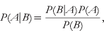
where P(A|B) is the probability of the candidate contact given the observation of the current peak and conversely for P(B|A), whereas P(B) is the prior probability of the peak. P(A) finally is the prior probability of the contact, calculated as follows.
Different classes are constructed depending on the amino-acid type, the residue separation and the secondary structure. The latter only in the ProtInfo approach (Hung & Samudrala, Reference Hung and Samudrala2006), where the prior probability for each class is then the proportion of such contacts in the database liable to interact via an NOE. KNOWNOE (Gronwald et al. Reference Gronwald, Moussa, Elsner, Jung, Ganslmeier, Trenner, Kremer, Neidig and Kalbitzer2002) on the other hand measures the distribution of distances from the database for each contact type and converts these to volume distributions. These are then used for each putative assignment in an attempt to identify a unique solution: one that has a high-enough probability to account for peak intensity in its entirety. While it is clear that such approaches are effective at ranking short-range above medium- and long-range assignments, the primary objective of ambiguity reduction is to select amongst several long-distance assignments. In this respect, the prior probabilities are not sufficiently discriminatory and no clear criterion for accepting or rejecting assignments emerges.
2.1.5 Ambiguous restraints
A key feature of an NOE-assignment protocol is its ability to deal with peaks with several assignment possibilities. Indeed, it is often the case – especially for larger proteins – that even the best filtering is unable to completely resolve all the ambiguities. The application of early algorithms (Güntert et al. Reference Güntert, Mumenthaler and Wüthrich1991, Reference Güntert, Berndt and Wüthrich1993; Mumenthaler & Braun, Reference Mumenthaler and Braun1995; Mumenthaler et al. Reference Mumenthaler, Güntert, Braun and Wüthrich1997; Duggan et al. Reference Duggan, Legge, Dyson and Wright2001) was thereby limited to cases where the number of unambiguous signals was sufficient to obtain an initial fold.
To overcome this obstacle, Michael Nilges (Nilges, Reference Nilges1993, Reference Nilges1995) proposed treating ambiguous peaks as an overlap of signals from all the n possible assignments (which, in fact, is almost never the case, but we shall see that this does not matter) and to set the constraint on the summed volume rather than on one of the individual components.

where VA is the total (ambiguous) peak volume and Vk is the volume associated with a particular assignment. In terms of distances, this becomes
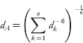
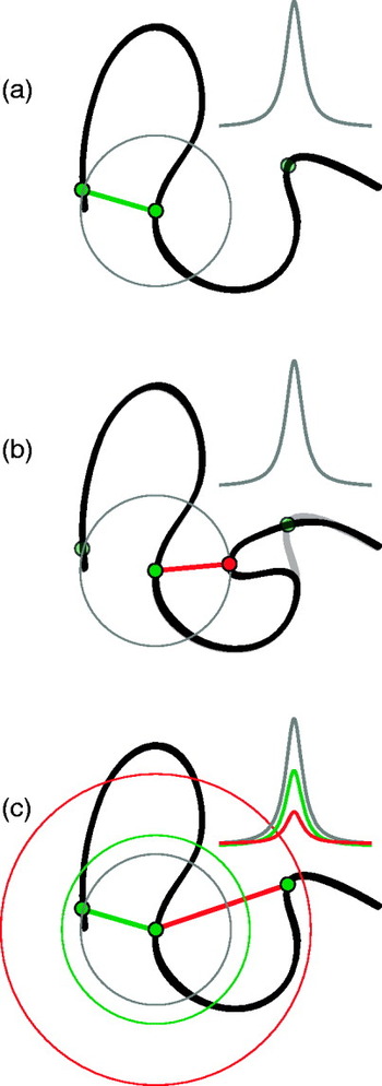
As illustrated in Fig. 5, because the intensity of the signal is inversely related to separation, ambiguous restraints are always laxer than those corresponding to the native structure. This means that the information is somewhat blurred out but more importantly, it guarantees that ambiguous constraints never distort a structure as long as the correct assignment is present. In fact, the concerted action of many ambiguous restraints during the molecular dynamics (MD) calculation forces each one to converge towards the correct unambiguous assignment. However, it is clear that this action becomes less and less effective as the average ambiguity increases. It is therefore vital that incorrect assignments be weeded out as much as possible prior to the constraints being set.
Illustration of the principle of ambiguous restraints for the case of two-fold assignment ambiguity. (a) The peak is unambiguously assigned to the correct candidate constraint. (b) The peak is unambiguously assigned to the wrong restraint, distorting the structure. (c) The peak volume is assumed to originate from both candidate contacts. An ambiguous restraint is applied such that the summed contribution from both assignments equals the experimental volume. Since constraints are applied as upper-distance limits, the correct structure is always fulfilled as long as the correct assignment is included.

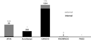
Histogram plot of the number of citations from PDB depositions for NOE assignment programs as of 27 August 2010. Citations from internal depositions are represented in black whereas those from external use of the program are shown in grey. In this context, we define internal depositions as those for which one or more of the developers appear as a structure author, or which originate from the same structural genomics project in which the program was developed. Exact search strings can be found in the Appendix, Table A2.

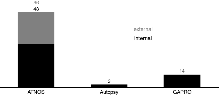
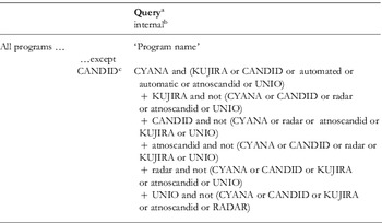
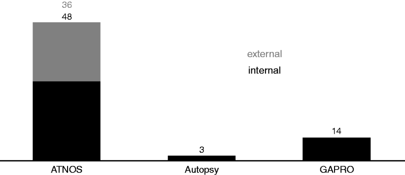
Histograms representing the number of citations from PDB depositions for peak picking algorithms as of 27 August 2010. Citations from internal depositions are represented in black, whereas those from external use of the program are shown in grey. In this context, we define internal depositions as those for which one or more of the developers appear as a structure author, or which originate from the same structural genomics project in which the program was developed. Exact search strings can be found in the Appendix, Table A3.
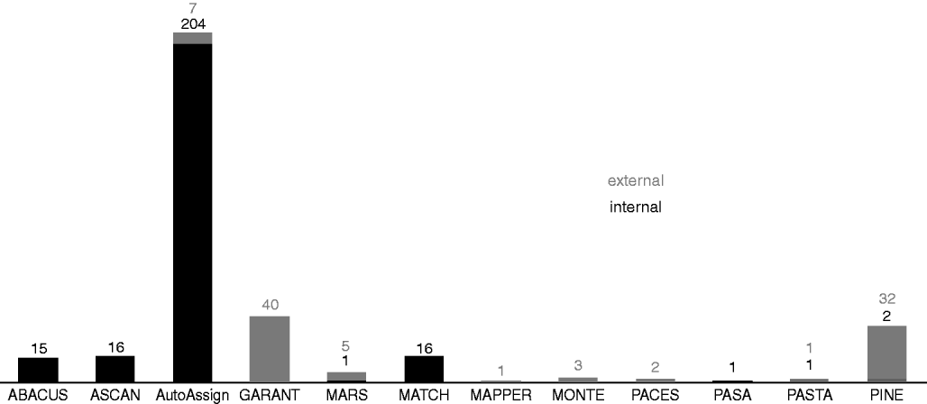
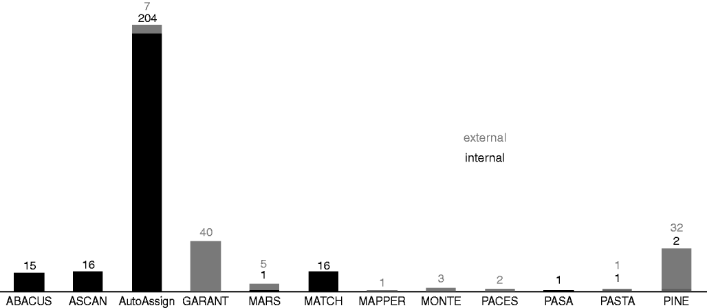
Histogram plot of the number of citations from PDB depositions for selected chemical shift assignment programs as of 27 August 2010. Only those programs are listed for which at least one citation was found. Citations from internal depositions are represented in black, whereas those from external use of the program are shown in grey. In this context, we define internal depositions as those for which one or more of the developers appear as a structure author, or which originate from the same structural genomics project in which the program was developed. Note that (Bermejo & Llinás, Reference Bermejo and Llinás2010) count 31 depositions for ABACUS. Exact search strings can be found in the Appendix, Table A1.
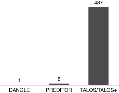
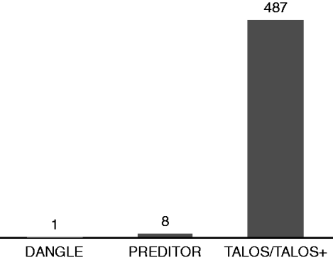
Histogram plot of the number of citations – as of 7 September 2010 – from PDB depositions for torsion angle-prediction software. Exact search strings can be found in the Appendix, Table A6.
2.1.6 Using intermediate structures: violation analysis
Once a preliminary structural model has been built, this can be used to re-evaluate the experimental data and filter assignments based on their agreement with the intermediate fold. Not only does this significantly reduce the initial chemical shift-based assignment ambiguity but it also identifies artefacts as the peaks with no structure-supported assignment. The difficulty, however, lies in identifying true violations from those caused by insufficient convergence or distortions caused by other artefacts. Violation analysis is therefore a double-edged sword; on the one hand, it ensures that the algorithms converge, but it makes it extremely hard to recover the native fold if this has not already been obtained after the first cycle. The algorithms are therefore heavily reliant on efficient, ab initio analysis of the experimental data.
As described above, ambiguous restraints are a means to let the MD algorithm decide which of the potential assignments should take precedent. Partial NOE assignment (Nilges & O'Donoghue, Reference Nilges and O'Donoghue1998; Linge et al. Reference Linge, O'Donoghue and Nilges2001; Kuszewski et al. Reference Kuszewski, Schwieters, Garrett, Byrd, Tjandra and Clore2004) aims at retrieving this information from the intermediate structures and may be used to supplement or replace (Kuszewski et al. Reference Kuszewski, Schwieters, Garrett, Byrd, Tjandra and Clore2004) violation analysis in reducing the assignment ambiguity.
For a given peak, the relative volume contributions from the list of candidate assignments are calculated according to the separation of the corresponding atoms in the latest structure. Usually, a cycle-dependent cut-off is imposed whereby initially, only very small contributions (long distances) are discarded with the selection criterion becoming more stringent after each cycle.
2.1.7 Eliminating artefacts
Experimental NMR spectra contain a substantial number of artefacts. As described above, intra-peak ambiguous restraints never distort a structure as long as the correct assignment is included. Artefacts clearly violate this rule and will lead to distortions. The risk being that these are carried through when intermediate structures are used to reassign the spectra. When working with unrefined peak lists, it is therefore critical to minimise the effect of artefacts even before the first structure is calculated.
Constraint combination (Herrmann et al. Reference Herrmann, Güntert and Wüthrich2002b) involves the implementation of inter-peak ambiguous restraints, which ensures a significant reduction in the number of artefacts. In the first stage, long-distance peaks are ranked according to their network anchoring and split into four categories from the most reliable quarter to the least. For each set of four peaks, one from each category, the most reliable is paired once with each of the three others, while the two middle-ranking peaks are combined to form the fourth ambiguous constraint. Thereby, a combined constraint will only distort the structure if both peaks are artefacts. The extent to which artefacts are suppressed depends on the initial proportion thereof and how well the network anchoring score reflects the true error probability of the peaks. For instance, the analysis of Herrmann et al. (Reference Herrmann, Güntert and Wüthrich2002b) shows that for a set of 1000 peaks of which 100 are artefacts and for which the top-ranked quarter is, respectively, twice and three times more reliable than the middle two and bottom-ranked quarters, only seven artefacts remain after constraint combination.
2.1.8 Distance calibration
In NMR protein structure determination, the peak volumes (or intensities) measured experimentally are converted to distance constraints under the two-spin approximation. As mentioned above, this simplification is rather drastic for proteins. In addition, it is actually quite difficult to accurately measure a peak volume in the presence of many overlapping lines. However, several factors contribute to the robustness of this approach. To begin with, because of the inverse power of six relationships, the NOE method is not sensitive to errors in the volume assessment. Furthermore, the distance constraints need not be precise as long as there are many and as long as conservative estimates (upper-distance limits) are taken. The remaining task is then to determine C, the spectrum-dependent constant, for which several methods have been proposed.
CANDID applies a continuous calibration whereby initially, peaks assigned to covalent contacts (for which the polypeptide structure imposes a maximal spatial separation such that an NOE is always expected) are used to calculate the calibration constant. In later cycles, the calibration constant is set such that no more than a given percentage (15 then 10%) of constraints violate the intermediate structure. AutoStructure (Moseley & Montelione, Reference Moseley and Montelione1999; Huang et al. Reference Huang, Tejero, Powers and Montelione2006) on the other hand, classes peaks according to their relative intensities before deriving upper-distance limits for each class.
A more precise interpretation of the information contained in the peak volumes may be achieved by back-calculating the experimental spectrum using the intermediate structure. Bardiaux et al. (Reference Bardiaux, Bernard, Rieping, Habeck, Malliavin and Nilges2009) have shown that the relaxation matrix (Ernst et al. Reference Ernst, Bodenhausen and Wokaun1987) approach employed in ARIA (Linge et al. Reference Linge, Habeck, Rieping and Nilges2004) effectively corrects for spin diffusion effects and results in tighter error bounds for the distance restraints. Understandably though, this more intricate approach is hungrier for computer resources.
2.1.9 Recent developments
The NOE-assignment programs mentioned above (see also Table 1 and Fig. 6), released roughly 10 years ago, are still in active development. A clear objective of the field in general is to make such tools more accessible to non-specialists. In this perspective, most programs now come complete with graphical user interfaces (GUIs). In fact, though the interpretation of the results is still the domain of experts, it reflects well on the maturity of the field that a virtual novice can set up and run a calculation in a matter of minutes.
To mention but a few examples, KUJIRA (Kobayashi et al. Reference Kobayashi, Iwahara, Koshiba, Tomizawa, Tochio, Güntert, Kigawa and Yokoyama2007) was developed as part of the RIKEN structural proteomics project (Yokoyama et al. Reference Yokoyama, Hirota, Kigawa, Yabuki, Shirouzu, Terada, Ito, Matsuo, Kuroda, Nishimura, Kyogoku, Miki, Masui and Kuramitsu2000a) to provide a graphical front end for CANDID with CYANA (Güntert, Reference Güntert2004) and to facilitate data management and analysis in the context of high-throughput structure calculations. Similarly, CANDID as part of UNIO and also ARIA now provide a number of graphical reports at the end of a structure calculation to facilitate the evaluation of the result. In addition, ARIA automatically performs energy refinement and reports on the quality of the structure obtained using several validation tools (see Section 2.2), as does AutoStructure with the recall, precision and F-measure (RPF) score (Huang et al. Reference Huang, Powers and Montelione2005). Finally, the software package AUREMOL (Gronwald & Kalbitzer, Reference Gronwald and Kalbitzer2004) associates KNOWNOE with graphical tools for NMR data processing and analysis.
2.1.10 Structure calculation and energy refinement
Being virtually unachievable manually or interactively, the building of atomic-resolution structure models was the first task to be successfully automated and indeed, this particular problem has been considered solved for the past 10 years or so. There is not much to add therefore to Peter Güntert's comprehensive review (Güntert, Reference Güntert1998) and the main programs (DYANA (Güntert et al. Reference Güntert, Mumenthaler and Wüthrich1997), CNS (Brunger et al. Reference Brunger, Adams, Clore, Delano, Gros, Grosse-Kunstleve, Jiang, Kuszewski, Nilges, Pannu, Read, Rice, Simonson and Warren1998), X-PLOR (Brunger, Reference Brunger1992; Schwieters et al. Reference Schwieters, Kuszewski, Tjandra and Clore2003)) have not changed significantly since then. Briefly though, in CYANA for example, the structure is obtained starting from an initially random fold by restrained MD simulations using a hybrid energy function that incorporates physical interactions and experimental constraints. For reasons of efficiency, the physical component in the target function is over-simplified, and therefore the final round of structure calculation should be followed by refinement using a physically realistic potential in explicit solvent (Güntert, Reference Güntert1998; Spronk et al. Reference Spronk, Nabuurs, Krieger, Vriend and Vuister2004; Nabuurs et al. Reference Nabuurs, Nederveen, Vranken, Doreleijers, Bonvin, Vuister, Vriend and Spronk2004a; Nederveen et al. Reference Nederveen, Doreleijers, Vranken, Miller, Spronk, Nabuurs, Güntert, Livny, Markley, Nilges, Ulrich, Kaptein and Bonvin2005). This is usually performed using force fields adapted from standard MD packages (Linge & Nilges, Reference Linge and Nilges1999; Koradi et al. Reference Koradi, Billeter and Güntert2000; Linge et al. Reference Linge, Williams, Spronk, Bonvin and Nilges2003; Case et al. Reference Case, Cheatham, Darden, Gohlke, Luo, Merz, Onufriev, Simmerling, Wang and Woods2005; Christen et al. Reference Christen, Hunenberger, Bakowies, Baron, Burgi, Geerke, Heinz, Kastenholz, Krautler, Oostenbrink, Peter, Trzesniak and Van Gunsteren2005; Phillips et al. Reference Phillips, Braun, Wang, Gumbart, Tajkhorshid, Villa, Chipot, Skeel, Kale and Schulten2005; Schwieters et al. Reference Schwieters, Kuszewski and Clore2006) but an alternative approach has recently been proposed, based on Rosetta structure prediction (Qian et al. Reference Qian, Raman, Das, Bradley, Mccoy, Read and Baker2007; Das & Baker, Reference Das and Baker2008; Ramelot et al. Reference Ramelot, Raman, Kuzin, Xiao, Ma, Acton, Hunt, Montelione, Baker and Kennedy2009). Protocols for energy refinement are constantly being updated and this improves structures past, present and future. A couple of recent studies have indeed demonstrated the value of amending prior depositions using the latest software (Nabuurs et al. Reference Nabuurs, Nederveen, Vranken, Doreleijers, Bonvin, Vuister, Vriend and Spronk2004a; Nederveen et al. Reference Nederveen, Doreleijers, Vranken, Miller, Spronk, Nabuurs, Güntert, Livny, Markley, Nilges, Ulrich, Kaptein and Bonvin2005): an excellent reason – if another were needed – to upload experimental restraints as well as the structure!
2.2 Structure validation
How confident can one be of the correctness of the structure obtained? There are two indirect criteria through which a structural biologist can address this most pertinent issue. First, does the structure truthfully represent the experimental data? Second, is the answer physically reasonable? Defining an NMR equivalent to the crystallographic R factor is problematic – low-quality data (e.g. few peaks) can easily lead to good scores, and therefore the latter question has made a more auspicious target (Spronk et al. Reference Spronk, Nabuurs, Krieger, Vriend and Vuister2004; Nabuurs et al. Reference Nabuurs, Spronk, Vriend and Vuister2004b; Snyder et al. Reference Snyder, Bhattacharya, Huang and Montelione2005).
As outlined in the previous section, a common source of problems is an incorrect balancing of experimental and electro-static potentials during structure calculation. Over fitting to experimental data can lead to unphysical structures, whereas under fitting leads to any number of unfolded random configurations. In general, force field tends to be biased towards experimental data notably through a simplification of the physico–chemical interactions. Over fitting is therefore much more common (Spronk et al. Reference Spronk, Nabuurs, Krieger, Vriend and Vuister2004; Nabuurs et al. Reference Nabuurs, Spronk, Vriend and Vuister2004b), which explains the requirement and power of refinement in explicit solvent (Nabuurs et al. Reference Nabuurs, Nederveen, Vranken, Doreleijers, Bonvin, Vuister, Vriend and Spronk2004a; Nederveen et al. Reference Nederveen, Doreleijers, Vranken, Miller, Spronk, Nabuurs, Güntert, Livny, Markley, Nilges, Ulrich, Kaptein and Bonvin2005). On the other hand, problems stemming from incorrect interpretation of experimental data are much more insidious, as even the most drastic errors prove difficult to characterise unambiguously (Nabuurs et al. Reference Nabuurs, Spronk, Vuister and Vriend2006; Saccenti & Rosato, Reference Saccenti and Rosato2008). Two recent studies are particularly informative on the ins and outs of validation in the context of automated protein structure determination.
In Nabuurs et al. (Reference Nabuurs, Spronk, Vuister and Vriend2006), an investigation of two abnormally differing depositions for homologous proteins leads to a search for similar anomalies in the PDB guided by commonly available validation software. (Note that structures deposited by structural genomics projects – where automation is prevalent – performed as well (or as badly) here as those from individual research groups: a cause for concern or celebration?) The authors use PROCHECK (Laskowski et al. Reference Laskowski, Macarthur, Moss and Thornton1993, Reference Laskowski, Rullmannn, Macarthur, Kaptein and Thornton1996) and WHAT IF (Vriend, Reference Vriend1990; Hooft et al. Reference Hooft, Vriend, Sander and Abola1996) to compare the local geometrical quality/normality of the homologues. Furthermore, the consistency of the experimental restraints is analysed by counting those that are violated while the QUEEN software (Nabuurs et al. Reference Nabuurs, Spronk, Krieger, Maassen, Vriend and Vuister2003) measures the information content of individual constraints. No single parameter unambiguously identified the erroneous structures. Rather, evidence was accumulated based on a residue-by-residue analysis of several quality scores and a constraint-by-constraint dissection of the experimental data.
In contrast, Edoardo Saccenti and Antonio Rosato (Saccenti & Rosato, Reference Saccenti and Rosato2008) are interested in how well different programs for structure validation (FRST (Tosatto, Reference Tosatto2005), HARMONY (Pugalenthi et al. Reference Pugalenthi, Shameer, Srinivasan and Sowdhamini2006), HOPPscore (Sims & Kim, Reference Sims and Kim2006), MolProbity (Lovell et al. Reference Lovell, Davis, Arendall, De Bakker, Word, Prisant, Richardson and Richardson2003), PROCHECK, ProsaII (Sippl, Reference Sippl1993; Wiederstein & Sippl, Reference Wiederstein and Sippl2007), TAP (Tosatto & Battistutta, Reference Tosatto and Battistutta2007), WHAT IF, all of which scrutinise physico-chemical quality) catch the increasingly serious mistakes (miss-calibrated and miss-assigned NOEs) they slip into the original set of experimental constraints. For a set of model proteins, the perturbed structures deviate by 2–3 Å from the reference without displaying obvious pathologies. In keeping with the results related above, the authors find that none of the tools reliably identify the distorted structures; the differences in particular scores between the erroneous and reference set are no larger than the variations within the latter.
It is well known that the tightness – or precision – of NMR structure bundles often overestimate their accuracy (Spronk et al. Reference Spronk, Nabuurs, Krieger, Vriend and Vuister2004). Nonetheless, this parameter is often assumed to be as meaningful as the X-ray resolution and is used as the primary gauge of structural quality. Saccenti and Rosato, however, find no correlation (positive or negative) between errors and precision, emphasising the perniciousness of this misconception.
The main conclusion to be drawn here from these studies is that as of yet, no simple protocol has been discovered for structure validation (see Table 2 for a list of available programs). On the contrary, a series of clues and pieces of circumstantial evidence must be gathered up painstakingly from all sources available. To this end, the software suites PSVS (Bhattacharya et al. Reference Bhattacharya, Tejero and Montelione2007) and CING (http://nmr.cmbi.ru.nl/cing/Home.html) assemble several existing tools within a single framework. The layperson may, however, be repelled by the somewhat bewildering array of scores, tests, reports and checks. In light of this, some programs output a single quality score. However, such summarising is obviously not conducive to the detailed inspection advocated above.
Solving the same structure twice using different sets of experimental data appears to be the fail-safe option, be this through cross-validation or by referring to a homologous protein. It is indeed exceedingly unlikely that the same mistakes are made twice. Unfortunately though, even a homology model does not allay the need for manual interpretation (Nabuurs et al. Reference Nabuurs, Spronk, Vuister and Vriend2006) and the experimental cost of complete cross-validation (RDCs are the preferred complement to NOEs) is often prohibitive.
2.3 Chemical shift assignment
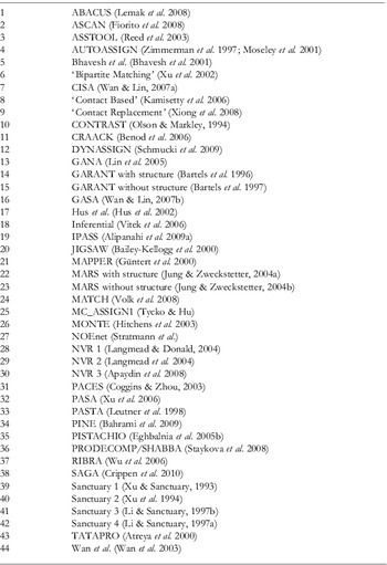
All the algorithms for NOE assignment described above require close to 100% backbone and side-chain chemical shift assignment for optimal performance. The shear number of methods published for automated chemical shift assignment is testament to the interest that this topic continues to attract. Perhaps the main driving force has been that even after 15 years or so of research, chemical shift assignment is seldom performed automatically as the tasks of manual assignment have proved difficult to implement systematically. The absence of a consensus procedure (notably in terms of the optimal set of experiments) highlights the difficulties in obtaining complete and reliable coverage. While scouring the literature in the context of writing this review, we have counted not less than 44 (more or less) novel automated procedures for backbone and/or side-chain assignment, published within the last 15 years or so. (The interested reader will find a list of these – undoubtedly not comprehensive – in the Appendix, and will find alternative compilations in the following reviews: Moseley & Montelione, Reference Moseley and Montelione1999; Baran et al. Reference Baran, Huang, Moseley and Montelione2004; Gronwald & Kalbitzer, Reference Gronwald and Kalbitzer2004; Bermejo & Llinás, Reference Bermejo and Llinás2010) In light of this, we will concentrate on certain representative algorithms to sum up the different approaches. Many ideas are indeed common to several programs, but expressed or implemented in a different way.
2.3.1 Generalities
Automated chemical shift assignment is usually performed in four stages with the aim first, to group resonances into spin systems; second, to determine the amino-acid type of each spin system; third, to create fragments from collections of spin systems that match sequentially; fourth, to associate the said fragments with a particular position in the amino-acid sequence. Usually at this stage, only the backbone and Cβ atoms are assigned (in the context of chemical shift assignment, the Cβ atoms are generally treated with the backbone atoms, rather than the side chain. In the following therefore, we use ‘backbone assignment’ to mean ‘backbone and Cβ assignment’) and indeed, the assignment of the side-chain atoms has proved even more problematic to complete automatically. A (smaller) number of algorithms have nonetheless been developed that include the side-chain atoms in the initial spin systems (stage one) (Bartels et al. Reference Bartels, Billeter, Güntert and Wüthrich1996, Reference Bartels, Güntert, Billeter and Wüthrich1997; Moseley & Montelione, Reference Moseley and Montelione1999; Baran et al. Reference Baran, Huang, Moseley and Montelione2004; Gronwald & Kalbitzer, Reference Gronwald and Kalbitzer2004). Alternatively, the two problems may be treated entirely separately with an algorithm dedicated to the side chains being applied (Fiorito et al. Reference Fiorito, Herrmann, Damberger and Wüthrich2008) once the backbone assignment has been completed.
The defining feature of most programs is their approach to mapping fragments onto the primary sequence (stage four), which involves finding the optimal combination amongst myriad possibilities. Most programs can thereby be classified accordingly as exhaustive search, best-first, Monte-Carlo or genetic algorithms.
2.3.2 AutoAssign
The best-first approach employed in AutoAssign (Zimmerman et al. Reference Zimmerman, Kulikowski, Huang, Feng, Tashiro, Shimotakahara, Chien, Powers and Montelione1997; Moseley et al. Reference Moseley, Monleon and Montelione2001) is perhaps the simplest to understand conceptually, if only because its description is jargon-free and does not require the assignment problem to be recast in terms of a more general theory. AutoAssign performs backbone assignment starting from a set of peak lists (five to eight) from traditional assignment experiments and information on amino-acid-specific chemical shift distributions extracted from the Biological Magnetic Resonance Bank (BMRB) (Doreleijers et al. Reference Doreleijers, Nederveen, Vranken, Lin, Bonvin, Kaptein, Markley and Ulrich2005). Following the approach outlined above, resonances from different spectra are aligned and grouped into dipeptide spin systems (stage one). At this stage, three classes are defined – distinct, overlapped and incomplete – for the spin systems depending on the ambiguity and/or completeness in terms of constituent resonances. The three subsequent steps are applied initially to the distinct class before exploiting the results to interpret and assign the overlapped and then incomplete spin systems. First, the amino-acid-type probabilities are determined for each dipeptide group (stage two) by comparing experimental chemical shifts with BMRB statistics. Then, spin systems are linked using a best-first approach. For each dipeptide, candidate neighbours are ranked according to the number of common resonances that match, and then according to the closeness of the match; the highest-ranking candidate is chosen and removed from subsequent consideration. Finally, the fragments of varying length are mapped to a unique position on the amino-acid sequence.
2.3.3 MATCH
In MATCH, the problem of sequence-specific backbone assignment is expressed in terms of the evolution of a set of individuals. The initial population is a set of sequence-specific resonance assignments (the individuals), each one built from fragments assembled from one or several APSY (Hiller et al. Reference Hiller, Fiorito, Wüthrich and Wider2005) spectra and arranged in a random sequence. In MATCH, a spin system consists of up to 18 frequencies (6 intra- and 12 inter-residue) linking two or three residues. The consolidation of resonances into spin systems is facilitated greatly by the numerous correlations already apparent in the high-dimensional APSY peak lists.
Starting with the longest fragments but otherwise randomly, these are removed from the buffer to the best-matching available position on the current individual. This procedure is repeated until a heterogeneous population is obtained, the size of which is determined automatically according to the ambiguity of the input data.
The evolutionary cycle proceeds through the independent mutation of each individual. Randomly, a fragment is chosen along with a new position where a swap is performed if at least one extremity of the candidate fragment fits with its neighbour. Furthermore, an assignment is made if the sequence-specific score – the chemical shift matching score between the experimental and predicted values, evaluated for the fragment at its new location, is above a given threshold. Conversely, if no compatible location is found after a given number of attempts, the process is re-initialised for a different candidate. However, those fragments that have already been assigned are locked in their positions.
This local optimisation is followed by an evaluation of assignments across the whole population. Temporary assignments are associated with a particular individual, whereas a permanent assignment is defined if a given temporary assignment is found in more than a predetermined fraction of the population.
Each cycle is punctuated by selective breeding whereby the genetic information from the fittest individuals forms a gene pool from which descendants are constructed. Specifically: in the first stage, the parent individuals are ranked according to their sequence-specific scores. This evaluates how well each fragment fits at its current position and the overall quality of the assignment. A buffer is then created using fragments from the highest-ranked individuals. As for the initial genesis, descendant individuals are constructed fragment by fragment from the gene pool, only now, the position of the fragments is inherited from the previous cycle.
The optimisation ends once all the individuals in the population are identical. The resulting assignment is then stored in a buffer of elite individuals and the whole procedure is repeated a predetermined number of times. An assignment is considered correct if it appears in more than 50% of the final elite population.
2.3.4 MARS
The emphasis so far has been placed on chemical shift assignment for de-novo NMR protein structure determination. In many cases, however, for instance when protein dynamics are of interest, a structural model already exists. The MARS procedure is original in that it can be augmented with a structural model and RDCs (Jung & Zweckstetter, Reference Jung and Zweckstetter2004a, Reference Jung and Zweckstetterb). Starting with the more conventional ‘chemical shift-only’ approach – which also forms the core of the ‘structure & RDC’ method – MARS relies on chemical shift and secondary structure prediction along with cumulative exhaustive searches to arrive at the correct assignment.
More precisely, a pseudo-energy is calculated for assigning a spin system to a particular position, based on how well the experimental chemical shifts match those expected from the primary structure. In MARS, the relevance of the comparison is enhanced by predicting the secondary structure of the protein using the program PSIRED (McGuffin et al. Reference Mcguffin, Bryson and Jones2000) and then using this information along with corrections for neighbouring residues to refine the chemical shift statistics from the BMRB. It should be noted that MARS requires spin systems rather than peak lists as input; i.e. stage one must be performed externally (manually or otherwise).
The MARS algorithm is constructed around an exhaustive search procedure initiated by allocating to all spin systems a random position in the amino-acid sequence. A spin-system is selected randomly and a forward search is performed along the sequence until all possible five fragments (fragments of five spin systems) have been constructed. The procedure for establishing sequential connectivities is tolerant for missing or imprecise data in that a putative link is only rejected if both common resonances are present and are in disagreement above a certain threshold. In contrast to best-first approaches (e.g. AutoAssign described above), candidate fragments are not ranked according to the quality of sequential match and all possibilities are considered at each stage of the exhaustive search. Each fragment is then placed at every possible position in the amino-acid list, the pseudo energy is calculated and a ranking is established. The lowest-energy five-fragment with its associated position identifies the best position for the optimal five-fragment starting from the initially selected spin system. Now, starting from the last residue of the highest-ranked fragment, the procedure is repeated in reverse. If again, the same five-fragment comes out on top associated with the same position, the initial spin system is relocated. This back and forth search is repeated until all spin systems have been used once as the root residue before re-initialising the cycle with four, three and two fragments. However, moving previously assigned spin systems comes with an extra energy cost. This ensures that correctly assigned residues are not repeatedly (and incorrectly) shifted around.
At this stage, a comparison is made between the fragment-derived assignments and the lowest pseudo-energy position for each spin system, analysed individually. Assignments are only conserved if they are found repeatedly in multiple runs. Indeed, the MARS procedure involves performing both assignment schemes 100 times during which Gaussian noise is added to the predicted shifts according to an empirically devised strategy. Assignments that are conserved in the first 20 pairs are kept fixed for subsequent rounds, then similarly for consistent assignments in the next 30, then again for the next 20 and the final 30. At each stage, the variance of the noise is reduced such that the most reliable assignments constrain the search for more uncertain attributions.
When RDCs and a structural model are provided, MARS proceeds in the same way except for an extra term in the pseudo energy that evaluates the match between RDCs measured experimentally and those back calculated from the structure. Since RDCs are very sensitive to small structural changes – that can occur for example due to dynamics, the RDC matching weighs less than the chemical shift. In addition, the alignment tensor is initially calculated using one of four possible methods and then the estimate is refined gradually as more assignments are made using singular value decomposition (SVD).
2.3.5 ABACUS
ABACUS (Lemak et al. Reference Lemak, Steren, Arrowsmith and Llinás2008) performs backbone and side-chain assignment using a traditional set of assignment experiments, minus those for establishing sequential connectivities. Indeed, in ABACUS, this information is extracted directly from the NOE spectra used subsequently for the structure calculation.
To begin with, NOEs are assigned to specific fragments using BACUS (Grishaev & Llinás, Reference Grishaev and Llinás2004; Lemak et al. Reference Lemak, Steren, Arrowsmith and Llinás2008) and the relative proximities of the later are determined from the resulting distance information according to the CLOUDS procedure (Grishaev & Llinás, Reference Grishaev and Llinás2002a).
ABACUS employs a multi-canonical MC algorithm (Berg & Neuhaus, Reference Berg and Neuhaus1991; Berg & Celik, Reference Berg and Celik1992) to find the minimum energy in the assignment space. The pseudo energy of the system has two components, the first of which accounts for the matching between the chemical shifts of the current fragment and those for the amino acid type at the candidate position, while the second evaluates whether the current fragment is close enough to its putative neighbour to form a sequential link. Thereby, the closer the two fragments are in the clouds (constructed in the previous cycle), the greater the number of NOEs connecting the pair (assigned by BACUS) and the higher the chemical shift similarity at the candidate position, the lower the energy.
During each MC run, fragment swaps are performed randomly and accepted if they lower the energy, or if they do not, with a probability

where E is the total energy of the system. Following a multi-canonical approach, the weight function S(E) is updated after each MC cycle such that
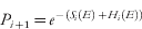
where Hi(E) is the energy histogram from MC run i. In addition, an absolute energy limit is imposed, which is reduced after each cycle; the idea in both cases being to push the sampling of assignment space towards low-energy regions.
2.4 Peak picking
Peak lists are the most common starting point for automated chemical shift or NOE assignment algorithms. It may seem surprising that the procedure of scanning a spectrum for maxima is still nowadays overwhelmingly performed manually. However, it turns out that NMR-based methods have extremely stringent requirements in terms of the accuracy of the picked peaks. Furthermore, it is extremely difficult to systematically distinguish between weak signals (which are often the most important) and artefacts. Consequently, and maybe also because of the convenience and intuitiveness of graphical interactive programs (Johnson & Blevins, Reference Johnson and Blevins1994; Bartels et al. Reference Bartels, Xia, Billeter, Güntert and Wüthrich1995; Neidig et al. Reference Neidig, Geyer, Gorler, Antz, Saffrich, Beneicke and Kalbitzer1995; Goddard & Kneller, Reference Goddard and Kneller2008), the peak-picking algorithms described in the following sections have not (yet?) become familiar tools for most spectroscopists. While an intimate coupling between peak picking and peak prediction has proved so far to be the most effective approach (Herrmann et al. Reference Herrmann, Güntert and Wüthrich2002b), a promising recent development has been to incorporate peak picking in the design of new NMR experiments (Korzhneva et al. Reference Korzhneva, Ibraghimov, Billeter and Orekhov2001; Orekhov et al. Reference Orekhov, Ibraghimov and Billeter2001; Hiller et al. Reference Hiller, Fiorito, Wüthrich and Wider2005; Eghbalnia et al. Reference Eghbalnia, Bahrami, Tonelli, Hallenga and Markley2005a).
2.4.1 AUTOPSY
AUTOPSY (Koradi et al. Reference Koradi, Billeter, Engeli, Güntert and Wüthrich1998) is a stand-alone method for automatic peak picking in the sense that it does not use any additional information to that which is contained in the spectrum. The main features of the program are an algorithm for local noise estimation, the segmentation of the spectrum into more-manageable chunks, the use of spectrum-specific peak templates and the exploitation of the intrinsic symmetry of magnetisation transfers.
Invariably, due to noise bands, water lines, artefacts, etc., the noise in NMR spectra is not evenly spread. The first stage of the AUTOPSY program involves calculating the average noise level for each 1D slice of the spectrum. The spectrum is then simplified by setting the intensity of pixels to zero if their value is below the local threshold. Next, the spectrum is split into connected regions using a flood-filling algorithm (Foley, Reference Foley1996). This ensures that even the most bulky multidimensional NMR spectra are treated efficiently. A set of reference line shapes is created by comparing the selections of well-resolved peaks from different regions. These templates are then used to resolve regions of strong overlap. Thereby, a peak – or rather a peak component – is accepted as a signal if a corresponding model can be found within the reference set. In addition, the presence of a symmetric peak, mirrored with respect to the spectrum diagonal is taken as an indication of the validity of a particular candidate.
2.4.2 ATNOS
The algorithm ATNOS was developed initially for combined NOE signal identification and protein structure calculation (Herrmann et al. Reference Herrmann, Güntert and Wüthrich2002b). It has subsequently been adapted for side-chain chemical shift assignment in combination with ASCAN (Fiorito et al. Reference Fiorito, Herrmann, Damberger and Wüthrich2008) and is used in APSY for the identification of projection peaks (Hiller et al. Reference Hiller, Fiorito, Wüthrich and Wider2005). ATNOS is designed to interface cyclically with assignment algorithms such that the selection criteria – and therefore the resulting peak lists – evolve as new assignments or more accurate structures become available. Updating the peak lists in this way ensures that the likelihood of an artefact being fed repeatedly to the assignment algorithm is much lower than if the peak picking were performed once only, as is common when signal identification is performed manually.
NOE assignment and structure calculation programs require essentially artefact-free peak lists. Indeed, it has been shown that when trading between accuracy and completeness, the former is much more valuable (Güntert, Reference Güntert2003; Jee & Güntert, Reference Jee and Güntert2003). To this end, ATNOS applies a series of increasingly stringent criteria for candidate resonances. Notably, and in contrast with other approaches, ATNOS makes extensive use of the information contained in the chemical shift assignments.
As a first step, all peaks whose intensities are no more than three times the AUTOPSY-calculated local noise level are removed. The covalent polypeptide structure imposes upper-distance limits on inter-nuclear distances. In ATNOS, these are calculated analytically for all proton pairs separated by fewer than two torsion angles. Correlations are expected for distances less than 5·5 Å. Candidate peaks whose coordinates match those for one of the predicted covalent signals form a reference set from which stricter area and intensity thresholds are defined.
The remaining peaks are divided into three classes: the reference or covalent set, peaks which are close to the diagonal and the rest. If no structural model is available, the ‘diagonal’ set is ignored. Peaks in the covalent set are accepted so long as they do not appear in a noise band, defined as an area in which the local noise level is more than three times the spectrum average. The remaining peaks must satisfy three additional criteria. First, the candidate peak must be well removed from others in the vicinity; if an area of noise does not separate it from its neighbours then the candidate peak must either be the most intense of the local group or be detached by a sufficiently deep intensity valley. Second, the candidate peak must have a symmetric double. Third, the candidate peak should be aligned with at least two peaks from the same plane (i.e. well anchored in the network of signals) and its coordinates should match at least one combination from the list of assigned atoms. If on the other hand, a preliminary structure is available, the grid of predicted signals is extended to all atoms within 5·5 Å and all peaks appearing close to an intersection are accepted. Those that do not satisfy this criterion are analysed as described above.
For ASCAN side-chain assignment, since the objective is to discover hitherto unknown assignments, rather than only accepting peaks at grid intersections where the nD coordinates are prescribed by the n interacting atoms, whole lines are considered as valid locations for peaks whereby the n−1 previously assigned chemical shifts provide the anchor points.
2.4.3 Noise reduction
Low signal-to-noise ratios are a clear obstacle to automated routines. A number of recently published methods aim at removing (some or most of) the noise in order to facilitate peak picking and render the process more robust.
The MICE (Serban, Reference Serban2007) protocol involves de-noising spectra using wavelet reconstruction (Daubechies, Reference Daubechies1992; Donoho & Johnstone, Reference Donoho and Johnstone1994, Reference Donoho and Johnstone1995; Mallat, Reference Mallat1999). Local maxima are then accepted above a certain threshold that is set relative to the average noise level in the spectrum. All line shapes are assumed to be Lorentzian and the average line width calculated from well-resolved peaks is then used to fit crowded regions.
Dancea & Gunther (Reference Dancea and Gunther2005) have investigated the effect of different de-noising algorithms on a 3D 15N-NOESY spectrum. The optimal schemes were then applied for the automated structure calculation of the polysulfide-sulfur transferase (Sud) protein (a homodimer with 2×137 residues), by which automatically picked peaks were fed into ARIA. Perhaps unsurprisingly, the more the noise level is reduced, the more spectral fine structure is lost. Consequently, two different de-noising schemes were employed during the structure calculation process. The most aggressive scheme was used to obtain a preliminary fold during five ARIA cycles and a spectrum that retained more weak features was analysed for four additional iterations. The final four cycles exploited a peak list extracted from the original spectrum. In contrast to the ATNOS protocol described above, each spectrum was analysed once only and no structure-based filters were used.
Within this framework, local maxima are accepted if they satisfy three criteria. First, they must be more intense than the local noise level (calculated as in AUTOPSY). Second, they must be supported by at least one different non-diagonal peak that is assignable to the same two residues (cf. network anchoring). And third, they must be supported by a symmetric double the other side of the diagonal.
An alternative approach has been proposed with PICKY, to remove noise using SVD (Alipanahi et al. Reference Alipanahi, Gao, Karakoc, Donaldson and Li2009b). Simple selection rules are then applied whereby the remaining noise is assumed to be evenly spread across the spectrum and maxima are accepted based on a minimum signal-to-noise threshold. Any additional spectra available are analysed in parallel such that depending on the type of experiment, signals originating from common atoms support each other.
2.4.4 Using new experiments
With many types of recently developed experiments, such as those based on reduced dimensionality or projections from higher-order dimensions (Malmodin & Billeter, Reference Malmodin and Billeter2005; Gryk et al. Reference Gryk, Vyas and Maciejewski2010), signals appear in standard patterns that can be analysed systematically in order to obtain peak lists. MUNIN (Korzhneva et al. Reference Korzhneva, Ibraghimov, Billeter and Orekhov2001; Orekhov et al. Reference Orekhov, Ibraghimov and Billeter2001) exploits the multi-dimensional decomposition (MDD) spectrum reconstruction procedure through which multi-dimensional (3D or higher) spectra are reconstructed from a set of model peaks. Peak positions are thereby obtained as a by-product, as it were, of the MDD process. APSY (Hiller et al. Reference Hiller, Fiorito, Wüthrich and Wider2005) experiments share the similarity with HIFI (Eghbalnia et al. Reference Eghbalnia, Bahrami, Tonelli, Hallenga and Markley2005a) that peak positions are extracted directly from projected spectra without reconstructing the multi-dimensional parent. In APSY, a simple peak picker is included to analyse 2D projections such that all maxima are accepted as long as they satisfy the local threshold criterion described above. Then, GAPRO repeatedly selects n−1 of the peak lists and back calculates peak positions in the n-dimensional spectrum. The resulting triangulation of individual peaks is highly redundant and therefore extremely precise. Similarly, although artefacts are picked in individual projections, these do not correlate during the GAPRO reconstruction, whereas signals do. Such approaches should prove particularly useful for providing peak lists for chemical shift assignments, for which high dimensionality is particularly valuable at tracing out sequential connectivities, as demonstrated for instance in the association of APSY with the MATCH algorithm for backbone assignment (Volk et al. Reference Volk, Herrmann and Wüthrich2008).
2.4.5 Integration
A number of proposals have also been made to interface peak picking of traditional experiments directly with chemical shift assignment algorithms. ATNOS/ASCAN for instance performs automated side-chain resonance assignment directly from NOESY or TOCSY spectra (Fiorito et al. Reference Fiorito, Herrmann, Damberger and Wüthrich2008). For backbone assignment, AUTOPSY has been interfaced directly with GARANT (Bartels et al. Reference Bartels, Güntert, Billeter and Wüthrich1997; Malmodin et al. Reference Malmodin, Papavoine and Billeter2003). Once the chemical shift assignment is complete, ATNOS/CANDID (Herrmann et al. Reference Herrmann, Güntert and Wüthrich2002a) is well established as a robust algorithm for constraint gathering directly from NOE spectra and a similar approach has been proposed by Dancea and Gunther with ARIA in the context of wavelet de-noised NOE spectra (Dancea & Gunther, Reference Dancea and Gunther2005).
Integration of the stages outlined in this section is a key objective in the ongoing quest for higher throughput and objectivity. At this stage, it seems that the mashups described above strike the optimal balance between efficiency and accuracy, and between time spent on data acquisition and analysis (see below). Indeed, a major obstacle for fully integrative approaches – in this context, those that read spectra and output a structure – is the cumulative propagation of errors.
The principle of fully automated NMR protein structure determination was first proven with the FLYA algorithm (Lopez-Mendez & Güntert, Reference Lopez-Mendez and Güntert2006); for three 12–16 kDa proteins the FLYA approach performed to a similar standard as traditional step-by-step automation. FLYA interleaves a series of well-established programs: peaks are picked automatically using NMRView (Johnson & Blevins, Reference Johnson and Blevins1994) or AUTOPSY; GARANT performs the chemical shift assignment while the overall process is controlled through the CYANA (Güntert, Reference Güntert2004) suite for NOE assignment and structure calculation; finally, energy minimisation is performed using OPALp (Koradi et al. Reference Koradi, Billeter and Güntert2000) with the AMBER (Case et al. Reference Case, Cheatham, Darden, Gohlke, Luo, Merz, Onufriev, Simmerling, Wang and Woods2005) force field.
Similarly, the FAPSY (Shin & Lee, Reference Shin and Lee2008) approach associates AutoAssign (Zimmerman et al. Reference Zimmerman, Kulikowski, Huang, Feng, Tashiro, Shimotakahara, Chien, Powers and Montelione1997; Moseley et al. Reference Moseley, Monleon and Montelione2001) for chemical shift assignment with TALOS (Cornilescu et al. Reference Cornilescu, Delaglio and Bax1999) and CYANA for constraint gathering and structure calculation. Applied to two proteins of 90 and 111 residues, the FAPSY protocol calculated structures that deviated from the reference by 3·2 and 3·0 Å, respectively.
There is a clear disadvantage with these methods, however, – if high-throughput is a concern – in terms of the number of spectra required and hence the experimental expenditure. In the original FLYA implementation, for instance, 16 spectra were used. Subsequent implementations of the FLYA algorithm for SAIL-labelled proteins (Kainosho et al. Reference Kainosho, Torizawa, Iwashita, Terauchi, Ono and Güntert2006) suggest that peak picking is the limiting step in the procedure; with this task being performed interactively, nine spectra were sufficient to calculate the N- and C-terminus of calmodulin and five for ubiquitin (Takeda et al. Reference Takeda, Chang, Ikeya, Güntert, Chang, Hsu, Huang and Kainosho2008; Ikeya et al. Reference Ikeya, Takeda, Yoshida, Terauchi, Jee, Kainosho and Güntert2009).
UNIO attempts to alleviate problems of cumulative errors by promoting user-intervention at the completion of each step. UNIO is composed of the assignment modules MATCH (Volk et al. Reference Volk, Herrmann and Wüthrich2008) and ATNOS/ASCAN (Fiorito et al. Reference Fiorito, Herrmann, Damberger and Wüthrich2008), respectively for the backbone and side-chain atoms, along with ATNOS/CANDID (Herrmann et al. Reference Herrmann, Güntert and Wüthrich2002a) for NOE constraint gathering and structure calculation (with CYANA, CNS or X-PLOR). The standard input requirements are three APSY (Hiller et al. Reference Hiller, Fiorito, Wüthrich and Wider2005) and three NOE spectra although the assignment process with MATCH has already been demonstrated with a single 6D APSY spectrum (Volk et al. Reference Volk, Herrmann and Wüthrich2008). As part of the JCSG's proteins structure venture, the UNIO protocol has led to the deposition of 19 structures (67–198 residues) in the past two years.
2.5 Limitations
A common criticism of the classical NMR approach to structure calculation is that it leads to poor-quality structures. (In this context, we insist on the distinction between a good-quality structure (i.e. in terms of the covalent geometry) and one that exhibits the correct fold.) Or rather, that it does not perform as well as X-ray diffraction in terms of physico-chemical standards (Doreleijers et al. Reference Doreleijers, Rullmann and Kaptein1998, Reference Doreleijers, Vriend, Raves and Kaptein1999; Ratnaparkhi et al. Reference Ratnaparkhi, Ramachandran, Udgaonkar and Varadarajan1998; Spronk et al. Reference Spronk, Linge, Hilbers and Vuister2002; Fan & Mark, Reference Fan and Mark2003; Laskowski, Reference Laskowski2003). In fact, most of these problems stem from the simplified physical energy terms used during the structure calculation steps and are efficiently redressed by appropriate energy refinement in explicit solvent (Güntert, Reference Güntert1998; Spronk et al. Reference Spronk, Nabuurs, Krieger, Vriend and Vuister2004). Such criticism is therefore outdated and efforts are ongoing to rectify previously deposited data (Nabuurs et al. Reference Nabuurs, Nederveen, Vranken, Doreleijers, Bonvin, Vuister, Vriend and Spronk2004a; Nederveen et al. Reference Nederveen, Doreleijers, Vranken, Miller, Spronk, Nabuurs, Güntert, Livny, Markley, Nilges, Ulrich, Kaptein and Bonvin2005). This issue emphasises, however, the modelling aspect of NMR protein structure determination. The results obtained should always be interpreted within the framework of the underlying model and with its limitations in mind.
In this context, it should be pointed out that all NMR data interpretation is performed – and the resulting structures interpreted – on the basis of a single rigid conformation. This is perhaps a surprising simplification and in a sense, a pity, since NMR as a technique is uniquely suited to the characterisation of both protein structure and dynamics (and thereby function). This problem is well known in the community (Kim & Prestegard, Reference Kim and Prestegard1989; Torda et al. Reference Torda, Scheek and Van Gunsteren1990; Lindorff-Larsen et al. Reference Lindorff-Larsen, Best, Depristo, Dobson and Vendruscolo2005; Markwick et al. Reference Markwick, Malliavin and Nilges2008), but so far, progress towards a unified description has mostly been made, as it were, from the dynamics side (Korzhnev et al. Reference Korzhnev, Salvatella, Vendruscolo, Di Nardo, Davidson, Dobson and Kay2004, Reference Korzhnev, Religa, Banachewicz, Fersht and Kay2010; Bouvignies et al. Reference Bouvignies, Markwick and Blackledge2007; Korzhnev & Kay, Reference Korzhnev and Kay2008; Baldwin & Kay, Reference Baldwin and Kay2009; Markwick et al. Reference Markwick, Bouvignies, Salmon, Mccammon, Nilges and Blackledge2009). Alternatively, one may rely more heavily on computer modelling (Case, Reference Case2002; Mackerell, Reference Mackerell2004; Markwick et al. Reference Markwick, Sprangers and Sattler2005; Hornak et al. Reference Hornak, Abel, Okur, Strockbine, Roitberg and Simmerling2006), but as of yet, the simulation of long time-scale (>1 μs) motions in proteins remains a challenging prospect (Hamelberg et al. Reference Hamelberg, Mongan and Mccammon2004; Elber, Reference Elber2005; Markwick et al. Reference Markwick, Malliavin and Nilges2008; van der Kamp et al. Reference Van Der Kamp, Shaw, Woods and Mulholland2008; Chiang et al. Reference Chiang, Hsu and Latombe2010).
The scope of the traditional NMR method is also limited, both in terms of its efficiency and its applicability to larger systems. Even with full-automation (or perhaps even more so) chemical shift assignment typically requires upwards of ten spectra and notwithstanding cryo-probes and high magnetic fields, NOE spectra are still relatively weak. A balance must therefore be struck between expediting the experimental step and facilitating robust data analysis, although progress has been made towards solving both problems at once (Hiller et al. Reference Hiller, Fiorito, Wüthrich and Wider2005, Reference Hiller, Wider and Wüthrich2008; Fiorito et al. Reference Fiorito, Herrmann, Damberger and Wüthrich2008; Volk et al. Reference Volk, Herrmann and Wüthrich2008). Systematic referencing across a large set of spectra – or rather the lack thereof – is also a problem. And while the internal calibration routines employed by most programs deal effectively with small discrepancies, meticulous manual referencing and alignment are prerequisites.
A more fundamental limit is the loss of resolution that follows the growth of targets – and ipso facto the number of peaks – as the corresponding slowing of protein motions leads to broader lines (Wüthrich, Reference Wüthrich1986; Neuhaus & Williamson, Reference Neuhaus and Williamson2000). To date, automated NOE assignment has been used to solve just one structure longer than 250 amino-acid residues (de Oliveira et al. Reference De Oliveira, Sforca, Blumenschein, Goldfeder, Guimaraes, Oliveira, Zanchin and Zeri2010) and more generally, structures heavier than 20 kDa are rarely targeted. In this instance, interactive data analysis is of little assistance (cf. Fig. 2). Perdeuteration is the traditional avenue towards accessing larger proteins and a number of selective labelling schemes have recently been proposed (Yee et al. Reference Yee, Gutmanas and Arrowsmith2006; Ohki & Kainosho, Reference Ohki and Kainosho2008; Shin & Lee, Reference Shin and Lee2008) – including notably the SAIL protocol (Ikeya et al. Reference Ikeya, Terauchi, Güntert and Kainosho2006; Kainosho et al. Reference Kainosho, Torizawa, Iwashita, Terauchi, Ono and Güntert2006; Takeda et al. Reference Takeda, Ikeya, Güntert and Kainosho2007b; Kainosho & Güntert, Reference Kainosho and Güntert2009), designed specifically with automation in mind – that promise to extend the range of classical NMR methods.
Of the steps involved, peak picking has proved to be the most troublesome to automate reliably. This is also the most critical stage as the dependability of the subsequent steps is underwritten by the accuracy of the peak lists provided. Indeed, the reliability of algorithms for chemical shift and NOE assignment deteriorates rapidly if more than a few artefacts are included. The latter also requires virtually 100% complete chemical shift assignment – of all NOE-interacting protons and their attached heavy atoms; i.e. a full record in terms of the NOE spectra rather than the primary structure (Güntert, Reference Güntert2003; Jee & Güntert, Reference Jee and Güntert2003), rarely available from the outset. Rather, the preliminary fold obtained from a subset of reliable signals is used to recursively complete chemical shift and then NOE attributions. This is possible because the network of NOE constraints is highly redundant meaning that this approach is robust with respect to peaks missed (or ignored).
3. Alternatives
NMR structural biology aspires to high throughput and objectivity. Automation of the different steps of the classical approach has gone some way to achieve these twin aims. As we have seen, though, some problems remain unsolved. A few radical approaches suggest that circumventing rather than overcoming the difficulties is the way forward.
Eliminating the need for chemical shift assignment is perhaps the most obvious short cut: this step of the traditional approach has no biological relevance and typically requires a huge investment in terms of experiments and data analysis. On the other hand, problems stemming from weak NOE spectra are the simplest to avoid as a number of NMR observables – notably chemical shifts and RDCs – are readily related to structural parameters. The methods described in this section follow this general philosophy although as we shall see, the border between classical and non-classical methods is not as clear-cut as might suggest the paradigm shift outlined above.
3.1 Chemical shift-based methods
The correlation between chemical shifts in proteins and their structure is well established, but complicated (Szilagyi, Reference Szilagyi1995; Wishart & Case, Reference Wishart and Case2001; Mielke & Krishnan, Reference Mielke and Krishnan2009; Mulder & Filatov, Reference Mulder and Filatov2010; Wishart, Reference Wishart2010). In contrast to NOEs or RDCs, there is no single equation to link this observable to a pairwise orientation or distance (with the exception of paramagnetic pseudo-contact shifts; Bertini et al. Reference Bertini, Luchinat and Parigi2001). Moreover, chemical shifts vary primarily with each nucleus’ local environment and depend only weakly on the non-covalent structure. Only recently have algorithms appeared that derive statistical predictions from ever-growing databases of structures and their corresponding chemical shifts (Wishart, Reference Wishart2010). (So the first stage of the traditional procedure is useful after all!) Two main classes of programs exist for which the output is either a set of torsion angles – to be used in conjunction with other restraints in subsequent structure calculation – or the query protein itself.
3.1.1 Torsion angle constraints
The programs for torsion angle constraints TALOS (Cornilescu et al. Reference Cornilescu, Delaglio and Bax1999), TALOS+ (Shen et al. Reference Shen, Delaglio, Cornilescu and Bax2009a), PREDITOR (Berjanskii et al. Reference Berjanskii, Neal and Wishart2006) and DANGLE (Cheung et al. Reference Cheung, Maguire, Stevens and Broadhurst2010) match sections of a target protein to those from a structural database based on their sequence and chemical shift similarity. The underlying idea is that a particular chemical shift pattern is indicative of a specific set of torsion angles. Thereby, if such a pattern from a query fragment can be matched to one in a database, so the corresponding torsion angles must also agree.
The overall strategy for each program being essentially identical, differences reside only in its implementation. A similarity score is calculated for each position in the amino-acid sequence, measuring the level of agreement between the chemical shifts of the query triplet (quintuplet in the case of DANGLE) and fragments of the same length from the database. A residue difference correction is applied, which separates primary and secondary structural influences on the chemical shifts. A parallel search is conducted based solely on sequence homology, which exploits the structural information intrinsic to the amino-acid sequence. The best results are then combined and the prediction is output along with a confidence rating or error estimate. TALOS+ and DANGLE also classify results based on favoured regions in Ramachandran plots (Ramachandran et al. Reference Ramachandran, Ramakrishnan and Sasisekharan1963).
To a first approximation, the larger the database, the more likely one is to find a match for a particular fragment and the more reliable are the predictions (Shen et al. Reference Shen, Delaglio, Cornilescu and Bax2009a). However, great care must be taken in constructing these databases such that the referencing for all chemical shifts is consistent. TALOS+ uses the 200-protein database constructed and calibrated as part of the SPARTA chemical shift prediction project (Shen & Bax, Reference Shen and Bax2007). A subset of this database (186 structures) forms the basis of the DANGLE approach for which Cheung et al. (Reference Cheung, Maguire, Stevens and Broadhurst2010) have investigated the effect of systematic miss-referencing in the query protein. For PREDITOR, the reference-correction module ensures consistency between experimental shifts and those in the associated database of 141 proteins.
In terms of output, the TALOSs and DANGLE predict the backbone φ/ψ angles only, whereas PREDITOR also includes estimates of the side chain χ1 and ω angles, thanks to a sequence homology analysis. Note in this context, the recent release of the PROMEGA software (Shen & Bax, Reference Shen and Bax2010), which employs a TALOS-like approach to predict Xaa-Pro peptide bond conformations (pre-proline ω angles).
In terms of performance, Cheung et al. (Reference Cheung, Maguire, Stevens and Broadhurst2010) report similar prediction accuracy – ca. 70–80% within 30° – for all methods with their DANGLE algorithm providing more realistic error estimates. David Wishart has recently sought an objective ranking by running each program for the same set of 33 proteins. PREDITOR made accurate (φ and ψ within 30°) predictions for approximately 10% more residues than DANGLE or TALOS (94% vs. ~85%).
The backbone restraints obtained using these programs are approximate and local. It is therefore not possible to reconstruct the full protein fold using these constraints alone and indeed, in situations where a dense network of NOE restraints is available, the information gained from torsion angles adds little to the precision. However, in situations where inter-atomic distances are harder to come by – for large proteins for example, or for solid-state NMR – these approaches come to the fore. To bypass NOE-type experiments completely though, different recipes are required of which angle predictions are nonetheless one of their main ingredients.
3.1.2 From structures to chemical shifts
The fundamentals of chemical shift prediction from structure are not within the scope of this review. Moreover, a thorough description of this topic has newly been published (Wishart, Reference Wishart2010). For the sake of protein structure determination, the reverse problem of predicting chemical shifts from existing structures is not a concern per se. However, they do allow much larger X-ray databases to be translated. This expansion of protein fold space turns out to be critical for the accuracy of algorithms for (full) structure calculation based (primarily) on chemical shift data (see the following section). Briefly therefore, programs for chemical shift prediction (we have censured 10, namely 4DSPOT (Lehtivarjo et al. Reference Lehtivarjo, Hassinen, Korhonen, Perakyla and Laatikainen2009), CamShift (Kohlhoff et al. Reference Kohlhoff, Robustelli, Cavalli, Salvatella and Vendruscolo2009), PROSHIFT (Meiler, Reference Meiler2003), PRSI (Wang, Reference Wang2004), SHIFTCALC (Iwadate et al. Reference Iwadate, Asakura and Williamson1999), SHIFTS (Xu & Case, Reference Xu and Case2001), SPARTA (Shen & Bax, Reference Shen and Bax2007), and SHIFTX/SHIFTX2 (Neal et al. Reference Neal, Nip, Zhang and Wishart2003; Wishart, Reference Wishart2010)) construct nucleus-specific contour maps that translate torsion angles into chemical shifts. In general, these structure-shift tables are assembled from a set of high-resolution X-ray structures for which chemical shifts are also available. These relationships are generally supplemented by semi-classical or quantum-mechanical calculations of physico-chemical effects (e.g. solvent exposure, peptide anisotropy, motional averaging, pH, temperature, etc.). Corrections for protein dynamics can also be made (Lehtivarjo et al. Reference Lehtivarjo, Hassinen, Korhonen, Perakyla and Laatikainen2009) and some programs make direct use of sequence homology (Meiler, Reference Meiler2003; Shen & Bax, Reference Shen and Bax2007). Thereafter, variations mainly concern the size and content of the reference database, the number and nature (which nuclei) of the predictions for each residue and of course, the implementation of the prediction algorithm.
As for torsion angles, David Wishart has measured the correlation between experimental chemical shifts and those predicted by the algorithms SHIFTX, SHIFTX2, CamShift, Shifts and ProShifts for a set of 61 high-resolution X-ray structures (Wishart, Reference Wishart2010). In terms of the different nuclei, Cβ predictions score highest on average (correlation coefficient ~0·99) and HN lowest (~0·69). In terms of the different programs, the correlation coefficients obtained with SHIFTX predictions are the highest on average (~0·95), and lowest with SHIFTS (~0·79).
3.1.3 From chemical shifts to structures
A structure defines a single chemical shift pattern, no unique solution exists to the reverse problem as many different global conformations can satisfy specific local arrangements. The recent development of accurate chemical shift prediction algorithms (see the preceding section) points towards an iterative solution to the problem whereby candidate structures can be ranked according to their chemical shift agreement with the query protein. To this date three methods, namely CHESHIRE (Cavalli et al. Reference Cavalli, Salvatella, Dobson and Vendruscolo2007), CS-Rosetta (Shen et al. Reference Shen, Lange, Delaglio, Rossi, Aramini, Liu, Eletsky, Wu, Singarapu, Lemak, Ignatchenko, Arrowsmith, Szyperski, Montelione, Baker and Bax2008b) and CS23D (Wishart et al. Reference Wishart, Arndt, Berjanskii, Tang, Zhou and Lin2008) have been published although a general pathway to low-resolution structures was first published by Gong et al. (Reference Gong, Shen and Rose2007) and already in 2001, the structure of ubiquitin was computed using chemical shift data exclusively (Wishart & Case, Reference Wishart and Case2001). The idea moreover of supplementing Rosetta structure prediction with experimental data dates from the turn of the century (Bowers et al. Reference Bowers, Strauss and Baker2000).
Chemical shifts are again used to scan a database of solved structures but compared to the programs for torsion angle prediction, alternative approaches are implemented for the subsequent reconstruction of the 3D fold. CS-Rosetta simply uses the fragments as a restricted (but much more relevant) database for a standard Rosetta (Das & Baker, Reference Das and Baker2008) calculation; CHESHIRE uses molecular fragment replacement based on Monte-Carlo substitution of candidate fragments; CS23D meanwhile assembles fragments based on simple matching criteria. Chemical shift matching along with a standard energy functional then guides the refinement of the coarse-grain CHESHIRE and CS23D models. Specific details of these protocols may be found in the following.
3.1.3.1 CHESHIRE
The first stage of the CHESHIRE protocol involves predicting the secondary structure of three and nine-residue fragments from the query protein. Bayesian inference is used to account for the propensity of certain groups of amino acids to form specific conformations. This complements a more conventional chemical shift matching test. The second stage involves collecting dihedral angle constraints in a TALOS-type approach, albeit with a larger database. The backbone fold is then reconstructed from the selected fragments using a Monte-Carlo swapping routine whereby the Metropolis condition (Metropolis et al. Reference Metropolis, Rosenbluth, Rosenbluth, Teller and Teller1953) is applied according to the level of agreement between SHIFTX-predicted and experimental chemical shifts. Side chains are then added to the 20000-strong group of models that is whittled down to 500 during two stages of energy/chemical shift refinement. A converged calculation is one for which the energy vs. root mean square deviation (RMSD) (to lowest-energy structure) landscape is strongly funnelled.
3.1.3.2 CS-Rosetta
As the name suggests, CS-Rosetta employs chemical shifts (experimental from the query protein and SPARTA-predicted from the structural database) to construct a database of relevant fragments that form the basis for the well-established Rosetta protocol for Monte-Carlo assembly based on sequence homology followed by high-resolution energy minimisation (Das & Baker, Reference Das and Baker2008). During the generation of the refined database, optimal accuracy is ensured on the one hand by comparing secondary chemical shifts (i.e. removing amino acid type bias), and on the other hand by accounting for uncertainties associated with the SPARTA predictions. Shen et al. (Reference Shen, Lange, Delaglio, Rossi, Aramini, Liu, Eletsky, Wu, Singarapu, Lemak, Ignatchenko, Arrowsmith, Szyperski, Montelione, Baker and Bax2008b) show that these high-quality fragments lead to convergence – which is tested using the familiar ‘funnelled landscape’ criterion mentioned above – in some of the cases where Rosetta (without chemical shifts) fails.
3.1.3.3 CS23D
Rosetta is also included in the CS23D protocol, but only as a ‘fail-safe’ alternative and with a restricted set of structures generated (500 vs. 10–20 000), the emphasis being placed on efficiency. In the hands of Wishart et al. (Reference Wishart, Arndt, Berjanskii, Tang, Zhou and Lin2008), CS23D solved the same structures ca. 10 000 times faster than CS-Rosetta or CHESHIRE notably through extensive homology modelling. Indeed, CS23D avoids time-consuming Monte-Carlo structure reconstructions by comparing and directly selecting outputs of three different database searches. Candidate fragments are found based on sequence homology and chemical shift matching (using SHIFTX-prediction for the structural database), but also according to torsion-angle homology after conversion of PREDITOR predictions to one of nine dihedral-angle labels. The backbone of the query protein may then be assembled by directly stitching fragments (with no limit on length) from one or other of the searches according to their relative success for a given stretch. The algorithm reverts to the restricted Rosetta run should the previous approach fail. In both cases, the procedure is completed by energy refinement in torsion angle space and a minimisation of chemical shift discrepancies.
3.1.3.4 Chemical shift restraints in MD simulations
The feasibility of the fragment assembly chemical shift methods was initially proven for ~10–20 small proteins (Cavalli et al. Reference Cavalli, Salvatella, Dobson and Vendruscolo2007; Wishart et al. Reference Wishart, Arndt, Berjanskii, Tang, Zhou and Lin2008; Shen et al. Reference Shen, Lange, Delaglio, Rossi, Aramini, Liu, Eletsky, Wu, Singarapu, Lemak, Ignatchenko, Arrowsmith, Szyperski, Montelione, Baker and Bax2008a). Since then, the application of CS-Rosetta and CHESHIRE protocols has been extended to situations where the chemical shift data for the query protein are incomplete (Robustelli et al. Reference Robustelli, Cavalli and Vendruscolo2008; Shen et al. Reference Shen, Vernon, Baker and Bax2009b). Owing to their database approach, however, all these approaches struggle to reproduce novel folds (Shen et al. Reference Shen, Lange, Delaglio, Rossi, Aramini, Liu, Eletsky, Wu, Singarapu, Lemak, Ignatchenko, Arrowsmith, Szyperski, Montelione, Baker and Bax2008a) and in this respect the CS23D suffers most having sacrificed flexibility for efficiency (Wishart et al. Reference Wishart, Arndt, Berjanskii, Tang, Zhou and Lin2008). In this case, why not use chemical shifts directly? Why not add a chemical shift term to an MD force field?
This is perhaps a more intuitive implementation of chemical shift restraints and efforts to incorporate these in the structure calculation process can be traced back to the early 1990s (Ösapay & Case, Reference Ösapay and Case1991; Ösapay et al. Reference Ösapay, Theriault, Wright and Case1994; Celda et al. Reference Celda, Biamonti, Arnau, Tejero and Montelione1995; Szilagyi, Reference Szilagyi1995; Kuszewski et al. Reference Kuszewski, Gronenborn and Clore1995a, Reference Kuszewski, Gronenborn and Cloreb, Reference Kuszewski, Qin, Gronenborn and Clorec; Clore & Gronenborn, Reference Clore and Gronenborn1998). However, these initial investigations were limited to refining structures that had already converged to the native state. Indeed, all but the tiniest conformational changes incur large (and often erroneous) energy penalties and imprecisions in chemical shift predictions only exacerbate this problem. Therefore, the large structural rearrangements required for a uniform sampling of conformation space are formidably difficult to provoke on the basis of chemical shift pseudo energies.
Recent improvements in the accuracy of the predictions have revived interest in the subject. Robustelli et al. (Reference Robustelli, Cavalli, Dobson, Vendruscolo and Salvatella2009) combined SHIFTX prediction with Monte-Carlo rearrangement governed by a physical potential with an extra term to penalise chemical shift discrepancies. While this approach suffered less from the limitations outlined above, still more than 90% of the random swaps were rejected, severely restricting the sampling of conformation space.
Contrary to other chemical shift prediction software, the functions output by CamShift are differentiable with respect to atomic coordinates which means that MC sampling can be replaced with MD simulations. Lately thereby, Robustelli et al. (Reference Robustelli, Kohlhoff, Cavalli and Vendruscolo2010) have upgraded their approach and successfully identified the native fold of 11 out of 12 small proteins starting from partially unfolded structures (56–108 residues, RMSD bias to reference 0·8–2·2 Å). De novo structure calculation is still not possible, however, as the MD simulations become trapped in local minima when starting from random structures. Loop regions are also problematic as errors in the CamShift predictions prevent otherwise valid conformational changes. At this stage, therefore, the authors suggest that CS-MD should be used in conjunction with other restraints or methods and indeed, they demonstrate the potential of CS-RDC-MD for the excited state peptide bound form of the Abp1p SH3 domain, with restraints obtained from relaxation dispersion experiments (Korzhnev et al. Reference Korzhnev, Salvatella, Vendruscolo, Di Nardo, Davidson, Dobson and Kay2004; Korzhnev & Kay, Reference Korzhnev and Kay2008; Baldwin & Kay, Reference Baldwin and Kay2009).
3.2 RDC-based methods
RDCs can be measured for proteins by placing samples in a liquid crystalline material, thereby limiting the tumbling that usually cancels out dipolar interactions in solution. RDCs constrain the dipole vectors of all atoms with respect to the same alignment tensor. As for NOEs, there is a direct theoretical link between experimental values and structural parameters (Bax et al. Reference Bax, Kontaxis and Tjandra2001; Prestegard et al. Reference Prestegard, Bougault and Kishore2004; Blackledge, Reference Blackledge2005):

The order parameter, S, is assumed constant; rij is the inter-nuclear distance oriented (θ, φ) with respect to the alignment tensor with axial and rhombic components Aa and Ar, respectively.
RDCs are, however, highly degenerate with respect to the alignment tensor (Ramirez & Bax, Reference Ramirez and Bax1998; Bax et al. Reference Bax, Kontaxis and Tjandra2001; Blackledge, Reference Blackledge2005; Donald & Martin, Reference Donald and Martin2009). The main concern of RDC-based algorithms is then to gather constraints in order to define a single reference frame. The traditional approach is to measure a specific set of RDCs – the more the merrier – in two alignment media. Despite being undesirable; because of the investment required in terms of sample preparation and experimental time, this is the only way to overcome the high degeneracy of the orientations of the peptide planes. Indeed, even multiple RDCs, but from a single alignment medium, leave many ambiguities unresolved and the additional information may only improve the precision of the structure bundle, rather than the accuracy of the atomic coordinates (Hus et al. Reference Hus, Salmon, Bouvignies, Lotze, Blackledge and Bruschweiler2008). An alternative is to use a database of known structures, NOEs and/or dihedral angle restraints to wipe out the degeneracies (Annila et al. Reference Annila, Aitio, Thulin and Drakenberg1999; Delaglio et al. Reference Delaglio, Kontaxis and Bax2000; Andrec et al. Reference Andrec, Harano, Jacobson, Friesner and Levy2002; Rohl & Baker, Reference Rohl and Baker2002). Note that for most methods (see Table 3 for a list), 15N enrichment is sufficient (optimal performance is nonetheless achieved with fully labelled samples); therefore, the extra complication of producing aligned samples is offset to an extent by a reduction in labelling costs. To reiterate though, no labelling strategy can circumvent the requirement of measurements in several alignment media.
It is clear, however, that an optimal set of restraints has not yet been defined. Indeed, depending on the availability of the different experimental constraints, any one of the algorithms described in the following may be the most favourable for a particular target. Another issue concerning software developed so far is that the measurement of RDCs is not as popular and widespread as say, NOEs; therefore, most programs have only been tested so far on simulated data (using e.g. PALES (Zweckstetter & Bax, Reference Zweckstetter and Bax2000; Zweckstetter et al. Reference Zweckstetter, Hummer and Bax2004; Zweckstetter, Reference Zweckstetter2008)) or experimental values recorded on model proteins.
Exploiting previously solved structures
Molecular fragment replacement (MFR)
Unlike NOE-based structure calculation algorithms, Monte-Carlo or simulated annealing-type methods do not regularly obtain native folds from RDC constraints, mainly because of local minima caused by degenerate solutions to global RDC restraints. This limitation does not, however, apply to elements of the structure; hence, the idea behind MFR (Annila et al. Reference Annila, Aitio, Thulin and Drakenberg1999) to reconstruct protein structures using the most likely fragments selected from a database.
In MFR, fragments from the query protein 7–10 amino acids in length are compared to those in a database of high-resolution X-ray structures (a subset of the PDB). The best 20 fragments are selected according to a χ2 fit to the experimental RDCs and to a lesser extent, the chemical shifts and primary structure. A dozen or so RDCs are required for each fragment, optimally measured in two alignment media. A similar approach has been proposed by Andrec et al. but using a single dataset (Andrec et al. Reference Andrec, Du and Levy2001; Andrec et al. Reference Andrec, Harano, Jacobson, Friesner and Levy2002). And indeed for favourable cases, MFR can also make do with fewer constraints (Kontaxis et al. Reference Kontaxis, Delaglio and Bax2005).
Small structural changes can lead to large variations in RDCs. Conversely, in order to whittle away these false positives, the top fragments are energy minimised with respect to the experimental RDCs by low-temperature simulated annealing. The selection is further refined by only accepting well-clustered fragments within the top 20. Any ambiguities are removed during the next stage of fragment assembly whereby sequential units are appended to the existing structure while minimising the RMSD to the latter. Subsequent appendages have many residues in common therefore in general overlapping fragments will have a single shared orientation. If however, this procedure does not converge to a single fold – axially symmetric alignment is a typical problem, the remaining ambiguities are easily resolved using a few specific NOE constraints.
In this arrangement, MFR solved both domains of the murine gamma-S crystalline (Wu et al. Reference Wu, Delaglio, Wyatt, Wistow and Bax2005) (PDB IDs: 1ZWM & 1ZWO) that were recombined with the help of small-angle X-ray scattering (SAXS) data (Grishaev et al. Reference Grishaev, Wu, Trewhella and Bax2005) (2A5M). In addition, the latest version of the program, MFR+, has been tested on both experimental and simulated data sets for six model proteins (sequence length 56–153 and ~4–5 RDCs per residue in two alignment media) (Kontaxis et al. Reference Kontaxis, Delaglio and Bax2005). The structures converged in all cases with backbone RMSDs to the reference structure in the range 0·44–1·95 Å.
3.2.1.2 RDC-Rosetta
We have already seen how experimental constraints – in this case chemical shifts, described in CS-ROSETTA section – can be used to increase the reliability of Rosetta structure predictions. Similarly, RDCs can be used to prune a database of the most relevant fragments and guide Rosetta backbone reconstruction towards low-energy regions of fold space (Rohl & Baker, Reference Rohl and Baker2002; Das & Baker, Reference Das and Baker2008).
Ten calculations were performed on simulated data from seven proteins and a converged structure, with a backbone RMSD below 3·0 Å was obtained in five cases. In addition, experimental RDCs were used for four model proteins, for which three converged to the native fold (backbone RMSD to the reference structure from 1·1 to 6·0 Å). In each case, highly homologous proteins were excluded from the database. Unsurprisingly, the more RDC restraints included, the more accurate was the Rosetta model.
3.2.2 Non-database methods
Since the theoretical link between NMR observable and structure is well-established in the case of RDCs, the tantalising prospect exists of accessing novel folds by calculating structures directly from the experimental values, thereby waiving the database homology requirement.
3.2.2.1 MECCANO
Planar arrangements of RDCs are eightfold degenerate with regard to a single alignment medium whereas chiral structures are fourfold degenerate. In two alignment media, the ambiguities are reduced by a factor of four meaning that as long as suitable chiral elements can be constructed, the orientation of the alignment tensor can be determined de novo (Blackledge, Reference Blackledge2005).
In MECCANO (Hus et al. Reference Hus, Marion and Blackledge2001), the six RDCs measured per residue, in two different alignment media define the peptide plane (Ni–Hi N, C′i−1–Ni, C′i−1–HiN, Cαi−1–C′i−1), and the tetrahedral trans-peptide bond (Cαi−1–Hαi, Cαi−1–Cβi−1). Together, these define the required sub-structure. For the calculation of ubiquitin, experimental values from two media were available for all couplings other than Cα–Cβ and totalled 648. The backbone RMSD between MECCANO and reference structures was 1·0 Å.
When data are missing for a particular plane, these can be simulated but the results are far less precise, hereby the prerequisite of extensive RDC constraints is the main limit for this approach. Note however, that of all the RDC-based programs described here, MECCANO is the only one to rely exclusively on such constraints. Since assigned chemical shifts are required anyway, dihedral angle constraints (Cornilescu et al. Reference Cornilescu, Delaglio and Bax1999; Berjanskii et al. Reference Berjanskii, Neal and Wishart2006; Shen et al. Reference Shen, Delaglio, Cornilescu and Bax2009a; Cheung et al. Reference Cheung, Maguire, Stevens and Broadhurst2010) could easily be incorporated into the protocol and thereby extend its applicability.
3.2.2.2 3P
Like MECCANO, the 3P algorithm (Wang et al. Reference Wang, Walsh, Kuszewski and Wang2007) constructs chiral elements from inter-nuclear vectors. However now, instead of relying on experiments in a second alignment medium, the degeneracy of the RDCs is lifted in regular secondary structure elements by exploiting periodic relationships between the coupling strengths and the orientation of the peptide planes (Mesleh et al. Reference Mesleh, Veglia, Desilva, Marassi and Opella2002; Lee et al. Reference Lee, Mesleh and Opella2003; Mascioni & Veglia, Reference Mascioni and Veglia2003; Mesleh et al. Reference Mesleh, Lee, Veglia, Thiriot, Marassi and Opella2003; Mesleh & Opella, Reference Mesleh and Opella2003; Walsh et al. Reference Walsh, Cabello-Villegas and Wang2004; Walsh & Wang, Reference Walsh and Wang2005). In addition, dihedral angle restraints are included to overcome problems if distinct solutions are not well defined – primarily ambiguities caused by missing or noisy data – and to constrain regions of non-regular secondary structure.
A Levenberg–Marquardt algorithm (Nocedal & Wright, Reference Nocedal and Wright2006) is used to fit peptide-plane orientations to the RDC data. The three best results are then considered during the fragment assembly stage. In a process similar to MFR, starting with the residues for which the most restraints are available, the backbone structure is reconstructed iteratively by appending each time the best-matching candidates in terms of RDCs.
The influence of imprecise or missing constraints has been investigated using data simulated for the protein cutinase (PDB ID: 1CEX). 3P remained robust with up to 30% noise added to the simulated RDCs (RMSD bias <3·0 Å) or with up to 30% of these missing (RMSD bias <2·5 Å). However, in the absence of (highly precise) dihedral angle restraints, the algorithm was not able to identify the correct fold (19 Å RMSD bias). For the three model proteins ubiquitin (1UBQ), GB3 (1IGD) and DinI (1GHH), also used to test the MFR+program, the performance of 3P is similar with backbone RMSDs to the reference structures of less than 1·0 Å.
3.2.2.3 RDC-PANDA
RDC-PANDA (Zeng et al. Reference Zeng, Boyles, Tripathy, Wang, Yan, Zhou and Donald2009) builds on recent work by Wang et al. (Wang & Donald, Reference Wang and Donald2004; Wang et al. Reference Wang, Mettu and Donald2006) to efficiently convert RDC measurements into structural constraints. The aim then is to connect RDC-defined secondary structure elements using unambiguous NOEs, and then to use this preliminary structure to re-evaluate the NOE spectra in the usual way. In this sense, RDC-PANDA has a lot more in common with early NOE-assignment algorithms (Güntert et al. Reference Güntert, Braun and Wüthrich1991; Güntert et al. Reference Güntert, Berndt and Wüthrich1993; Mumenthaler et al. Reference Mumenthaler, Güntert, Braun and Wüthrich1997) than with the other programs discussed in this section. It also shares their weakness in terms of assignment ambiguity and applicability for larger proteins. The extra experimental effort is therefore not justified and faced with the choice, it is clear that one would forgo the measurement of RDCs and opt for one of the more robust and proven NOE-assignment algorithms described in the previous section.
3.2.3 Combined chemical shift assignment and structure determination
On the other hand, the recording of RDCs as an alternative to chemical shift assignment is an alluring prospect. Note that the methods described so far in this section all require chemical shift assignment. As mentioned above, this process is notoriously labour-intensive and uncongenial to traditional automatic approaches.
3.2.3.1 ITAS and FastNMR
In ITAS (Jung et al. Reference Jung, Sharma and Zweckstetter2004), chemical shift assignment is performed automatically using MARS, first without and then with a structural model as the two rounds are interspersed with Rosetta structure prediction. Rosetta fragment assembly is however, notoriously slow and is prone to errors for larger proteins (>~100 residues) or novel folds (Bradley et al. Reference Bradley, Misura and Baker2005; Raman et al. Reference Raman, Lange, Rossi, Tyka, Wang, Aramini, Liu, Ramelot, Eletsky, Szyperski, Kennedy, Prestegard, Montelione and Baker2010b). In FastNMR (Korukottu et al. Reference Korukottu, Bayrhuber, Montaville, Vijayan, Jung, Becker and Zweckstetter2007), the second Rosetta step is replaced by a CYANA-MARS-CYANA sequence to complete the chemical shift assignment and refine the structure. FastNMR is therefore more robust and computationally efficient than ITAS, but incurs an extra experimental cost in the form of NOE spectra.
ITAS has been tested on a combination of experimental and simulated data from eight proteins (56–153 residues) (Jung et al. Reference Jung, Sharma and Zweckstetter2004). Out of ten calculations, seven were successful with backbone RMSD biases less than 3·0 Å. MARS was the culprit for the two Z domain (PDB ID: 2SPZ) runs. For DinI (1GHH), ITAS (Rosetta) was unable to obtain the correct fold even starting from previously published assignments. Starting from experimental data, the FastNMR approach on the other hand yielded high-resolution models of the proteins ubiqutin (1D37), Conk-S1 (2CA7) and Conk-S2 (Korukottu et al. Reference Korukottu, Bayrhuber, Montaville, Vijayan, Jung, Becker and Zweckstetter2007). In each case, the RMSD to the mean of the CYANA bundle was less than 1 Å as was the deviation from the reference structure (not available for Conk-S2).
3.3 RosettaNMR
It is clear that both RDC- and chemical shift-based protein structure determination is still in its infancy and the methods described over the last few pages cannot match the range or the robustness of the more mature NOE-based algorithms. But this is to be expected since the new algorithms have to make do with sparser (RDCs) or more approximative (chemical shifts) restraints.
To overcome these limitations and with the aim of establishing a rival protocol for the most challenging protein structures, a couple of recent studies have focused on different variations of RosettaNMR (Rohl, Reference Rohl2005; Raman et al. Reference Raman, Huang, Mao, Rossi, Aramini, Liu, Montelione and Baker2010a, Reference Raman, Lange, Rossi, Tyka, Wang, Aramini, Liu, Ramelot, Eletsky, Szyperski, Kennedy, Prestegard, Montelione and Bakerb). NMR constraints can either be used in advance – as it were – to filter the Rosetta database fragments (as described above for CS- and RDC-Rosetta), during the assembly process, to guide the sampling towards low energy regions of conformation space, or subsequently, to rank the resulting structures according to how well they reproduce the experimental data (Rohl, Reference Rohl2005).
3.3.1 CS-DP-Rosetta
We have seen that NMR peak picking is hard to perform automatically and that NOE-assignment algorithms are extremely sensitive to artefacts. In the course of most NMR protein structure calculations therefore, a lot of time is spent manually refining peak lists. One option to expedite this process is simply to avoid it. However, methods such as CS-Rosetta are only effective for small proteins. As a compromise therefore between efficiency and robustness, Raman et al. propose to filter CS-Rosetta models against NOE peak lists, thereby achieving the range of traditional NOE-assignment algorithms but with raw (or ‘minimally edited’) peak lists (Raman et al. Reference Raman, Huang, Mao, Rossi, Aramini, Liu, Montelione and Baker2010a).
The thousand or so lowest-energy CS-Rosetta models out of an initial set of 50 000 are filtered against the NOE peak lists using the RPF software (Huang et al. Reference Huang, Powers and Montelione2005). This evaluates how well a structure explains the experimental peak pattern. The top 20 conformers (energy+DP score) are then extensively refined according to the Rosetta ‘rebuild and refine’ protocol (Qian et al. Reference Qian, Raman, Das, Bradley, Mccoy, Read and Baker2007; Ramelot et al. Reference Ramelot, Raman, Kuzin, Xiao, Ma, Acton, Hunt, Montelione, Baker and Kennedy2009). When refined peak lists are available, an alternative strategy, ‘AssignNOE-Rosetta’ is to use a traditional NOE-assignment algorithm to produce a preliminary structure subsequently refined using Rosetta.
The CS-DP-Rosetta protocol was tested on six proteins, ranging in length from 97 to 145 amino acids. Three of these calculations were performed blind (i.e., without knowledge of the reference structure). Only in one case, surprisingly for the smallest protein, was the RMSD bias to the reference structure greater than 3·0 Å (Raman et al. Reference Raman, Huang, Mao, Rossi, Aramini, Liu, Montelione and Baker2010a). Moreover, AssignNOE-Rosetta performed systematically better than CYANA or AutoStructure with refined peak lists: for a set of five proteins (100–160 amino acids) the RMSD biases for the structured regions were in the range 1·0–1·4 Å as compared to 1·3–2·5 Å for the reference calculations (Raman et al. Reference Raman, Huang, Mao, Rossi, Aramini, Liu, Montelione and Baker2010a).
One would need to weigh up the extra computational cost incurred through the use of Rosetta (each CS-Rosetta model takes ~5–10 CPU minutes to build (Shen et al. Reference Shen, Lange, Delaglio, Rossi, Aramini, Liu, Eletsky, Wu, Singarapu, Lemak, Ignatchenko, Arrowsmith, Szyperski, Montelione, Baker and Bax2008b)) and the time-cost of manual peak-list refinement. Or perhaps a more relevant comparison could have been made with the ATNOS/CANDID protocol for (unsupervised) automatic peak picking and NOE assignment. Nonetheless, these results suggest that CS-DP-Rosetta is a viable alternative to the traditional NOE algorithms for medium-sized proteins.
3.3.2 CS-RDC-(NOE)-Rosetta
A different strategy has been proposed for larger proteins. Fig. 2 shows that for proteins longer than 200 residues solution NMR in general, and automated algorithms in particular are not a popular choice. Raman et al. seek to address this problem by supplying Rosetta with backbone chemical shifts and sparse NOEs (Raman et al. Reference Raman, Lange, Rossi, Tyka, Wang, Aramini, Liu, Ramelot, Eletsky, Szyperski, Kennedy, Prestegard, Montelione and Baker2010b). The authors argue that by exclusively using experimental constraints from the protein backbone, this approach should be more conducive to solving larger targets for which deuteration significantly reduces the density of the NOE network.
CS-Rosetta is robust up to approximately 100 residues. Adding RDC restraints to guide the conformational search towards low-energy regions (Rohl & Baker, Reference Rohl and Baker2002) helps CS-RDC-Rosetta to consistently solve structures up to a length of 120 amino acids (Raman et al. Reference Raman, Lange, Rossi, Tyka, Wang, Aramini, Liu, Ramelot, Eletsky, Szyperski, Kennedy, Prestegard, Montelione and Baker2010b). To push the size limit even further, backbone amide NOEs (HN–HN) were included at the ‘rebuild and refine’ stage (Raman et al. Reference Raman, Lange, Rossi, Tyka, Wang, Aramini, Liu, Ramelot, Eletsky, Szyperski, Kennedy, Prestegard, Montelione and Baker2010b). This CS-RDC-NOE-Rosetta protocol was tested for 15 proteins (122–266 residues) such that 13 structures were obtained that had converged for more than half of the sequence. Of these, ten had an RMSD bias to the reference structure of less than 3·5 Å (Raman et al. Reference Raman, Lange, Rossi, Tyka, Wang, Aramini, Liu, Ramelot, Eletsky, Szyperski, Kennedy, Prestegard, Montelione and Baker2010b).
This approach is advantageous since no experimental information is required for the side-chain atoms as these are added automatically during the refinement stage. Rosetta is not in the business of proving free lunches however: according to this study, the calculation of a 200 amino-acid protein takes in the order of 82 000 CPU hours. In terms of range and robustness moreover, it is not clear that CS-RDC-NOE-Rosetta actually constitutes an improvement on pre-existing methods.
3.4 Structure calculation with unassigned chemical shifts
Although efforts have concentrated so far on overhauling the traditional constraint-gathering paradigm, it can be argued that the most problematic and time-consuming step in NMR protein structure determination is chemical shift assignment and that efforts should on the contrary concentrate on eliminating this stage. Indeed, no standard approach has yet emerged – either in terms of experiments or algorithms – for automatic chemical shift assignment. An attractive proposition is to rely solely on the distance information contained in NOE spectra.
3.4.1 CLOUDS
Indeed, these always encode the spatial arrangement of protons in terms of correlated frequencies, whether the latter have been attributed to specific atoms or not. The pioneering work on this subject dates from the early 90 s (Malliavin et al. Reference Malliavin, Rouh, Delsuc and Lallemand1992) but so far, these ideas have only been pursued by a couple of research groups (Atkinson & Saudek, Reference Atkinson and Saudek1997, Reference Atkinson and Saudek2002; Grishaev & Llinás, Reference Grishaev and Llinás2002a, Reference Grishaev and Llinásb). Of the algorithms proposed, CLOUDS is the only one to have been successful starting from experimental data. For two small proteins (60 & 83 residues), the CLOUDS approach yielded backbone structures with less than 1·5 Å RMSD from the reference (Grishaev & Llinás, Reference Grishaev and Llinás2002a).
Parallels may be drawn between CLOUDS and X-ray methods for protein structure determination, in that NOESY spectra are used to create a spatial distribution (of protons here, rather than electrons) into which a model structure is then fit. Upper- and lower-distance constraints are extracted from the NOE spectra by relaxation matrix analysis. An MD simulation is then performed with electrostatic repulsions to assemble 1000 proton clouds. The candidates that deviate most from the mean are then discarded and the resulting family of clouds defines a sleeve into which the covalent structure is folded. Sequential connectivities are established through the clouds based on the likelihood of HN–HN, Hα–HN and Hα–Hα contacts obtained from a Bayesian interpretation of database values. A similar approach is used to attach the side chains. Finally, the fully assembled protein is squeezed into shape using MD constrained by the proton density.
A variation on the CLOUDS protocol has recently been proposed (Bermejo & Llinás, Reference Bermejo and Llinás2008). SC-CLOUDS is designed to work with selectively labelled perdeuterated proteins and uses Rosetta to assemble the final structure. Rosetta is required because the distance constraints are too sparse to collapse the proton clouds down to a single structure. SC-CLOUDS borrows this approach – roughly speaking: to use Rosetta instead of assigned chemical shifts – from the work of Jens Meiler and David Baker (Meiler & Baker, Reference Meiler and Baker2003), and we have seen that ITAS employs a similar strategy. We refer the interested reader to the comparison of these three methods in (Bermejo & Llinás, Reference Bermejo and Llinás2010).
4. Outlook
Perhaps one of the main conclusions to be drawn from this whole discussion is that when attempting to hasten the process of protein structure determination it is very hard to avoid gathering long-range constraints in general, and NOE distance limits in particular: one will have noted the use of NOE restraints to improve the robustness of many of the non-classical methods.
None of the protocols proposed as an alternative to classical NMR structure calculation have (yet?) imposed themselves in the field. This is maybe a question of maturity more than anything: the more established protocols have been gradually refined over more than ten years and extensively tested. Of all the algorithms available to the community for the automatic analysis of NMR data, only a limited number of NOE-assignment programs are routinely used.
When predicting the future state of a research field, a tempting manoeuvre consists in comparing the limitations of a rival approach, five-years-old, with the potential of one's own method, five years hence. Suffice to say here that since all the procedures come with specific advantages and drawbacks, and since most of the algorithms described so far are still in active development, the field seems destined to remain as vibrant as ever. In this context, we shall now briefly cover some emerging or related research topics that could influence automated NMR protein structure determination in the years to come.
4.1 Towards more realistic structure models
A structure should always be interpreted in the context of the assumptions and limitations of the modelling process. In NMR for example, the experimental data are invariably indirect, incomplete, insufficient and imprecise. Wherefrom stem four questions, namely; how accurate is the intensity–distance mapping? How ambiguous are the experimental constraints? How should they be weighted relative to physical parameters and how can the errors be quantified? By formulating protein structure determination as a problem of Bayesian inference, inferential structure determination (ISD) seeks objective rather than ad hoc answers (Rieping et al. Reference Rieping, Habeck and Nilges2005; Habeck et al. Reference Habeck, Nilges and Rieping2005a; Rieping et al. Reference Rieping, Nilges and Habeck2008).
It is illogical, the authors argue, to interpret NMR data on the basis of a single structure (as is done at present) if the former are uncertain. A Bayesian interpretation is preferable because it naturally accounts for all possible solutions and leads to an objective measure of the precision of a structural ensemble – the width of the probability distribution – based on the inferred accuracy of the experimental constraints (Rieping et al. Reference Rieping, Habeck and Nilges2005; Habeck et al. Reference Habeck, Nilges and Rieping2005a).
ISD is based on a Markov chain Monte Carlo algorithm (Habeck et al. Reference Habeck, Nilges and Rieping2005b) wherein, rather than keeping intensities and their calibration fixed, these parameters are sampled randomly and iteratively with conformation space to infer the errors, both experimental (for the intensities) and theoretical (for the distance calibration). Potential structures are represented by a posterior probability distribution of conformers given the experimental data and prior information (e.g. the covalent geometry). A replica exchange (Swendsen & Wang, Reference Swendsen and Wang1986; Earl & Deem, Reference Earl and Deem2005) approach ensures that the calculation does not become trapped in local minima.
So far, ISD has been used to calculate meaningful errors on atomic coordinates (Rieping et al. Reference Rieping, Habeck and Nilges2005) and to optimise the balance between experimental and theoretical constraints (Habeck et al. Reference Habeck, Rieping and Nilges2006). The same authors have also applied a similar procedure to calculate torsion angles from J couplings (Habeck et al. Reference Habeck, Rieping and Nilges2005c) and for the analysis of RDCs (Habeck et al. Reference Habeck, Nilges and Rieping2008). Even though this approach needs to be tested in more challenging situations, the prospect of more objective structures is alluring, if only to obviate lengthy cross validation and provide a true measure of NMR resolution.
Still, even ISD assumes that the experimental data can be explained by a single structure. By interfering with the NOEs, internal dynamics do contribute to the width of the ISD distribution, but this reflects uncertainties in the fold caused by a lack of information rather than true protein motions.
4.2 New frontiers for automated protein structure determination
To this date, a key influence on the development of algorithms for automatic protein structure determination has been the demand for high throughput in the ultimate aim of mapping out a sizeable fraction of protein fold space (Levitt, Reference Levitt2009; Terwilliger et al. Reference Terwilliger, Stuart and Yokoyama2009). It now seems that structural genomics is moving into a new age where the emphasis will shift from quantity to quality. The latest PSI initiative for example, PSI:Biology, seeks to foster tighter interplay between the structural and functional aspects of biology, as already done by other centres such as the SGC (Structural Genomics Consortium) and the Targeted Proteins Research Program (TPRP) (Ledford, Reference Ledford2010). This means that rather than choosing targets based mainly on their amenability to automatic calculation, selections will be made according to the current interests of the biological community, notably in terms of drug development. The implications for automated structure determination are numerous.
We have already mentioned two approaches geared specifically towards large proteins, combining selective labelling and extensive automation (Takeda et al. Reference Takeda, Ikeya, Güntert and Kainosho2007a; Raman et al. Reference Raman, Lange, Rossi, Tyka, Wang, Aramini, Liu, Ramelot, Eletsky, Szyperski, Kennedy, Prestegard, Montelione and Baker2010b). More challenging targets mean that a more generalised implementation of innovations – technical, experimental and in terms of sample preparation and data processing – will probably be required. These in turn will surely require new tools for automatic data analysis and interpretation.
Of course, NMR is not a panacea. In situations where high-quality crystals are readily obtained, NMR will continue to play second fiddle to faster methods based on X-ray diffraction. And in terms of protein sizes, the range of crystallography is unrivalled. However, structures in the PDB, solved both by NMR and crystallography, are intrinsically more reliable than those determined by one or other method (see validation section). This is particularly important as these databases are widely used for homology modelling and in general, for all fragment assembly methods. It is crucial therefore that the confidence in the structures should be maximised. In addition, small differences are interesting in terms of the behaviour of proteins in the two environments.
Alternatively, two sets of experimental data may be integrated directly in the structure calculation process. Automatic treatment of data from a number of sources can be modelled on programs for the prediction of protein interactions. For instance, a number of recent studies have demonstrated the value of combining SAXS and NMR restraints (Grishaev et al. Reference Grishaev, Wu, Trewhella and Bax2005, Reference Grishaev, Tugarinov, Kay, Trewhella and Bax2008a, Reference Grishaev, Ying, Canny, Pardi and Baxb; Gabel et al. Reference Gabel, Simon, Nilges, Petoukhov, Svergun and Sattler2008; Wang et al. Reference Wang, Zuo, Yu, Byeon, Jung, Wang, Dyba, Seifert, Schwieters, Qin, Gronenborn and Wang2009; Jehle et al. Reference Jehle, Rajagopal, Bardiaux, Markovic, Kuhne, Stout, Higman, Klevit, Van Rossum and Oschkinat2010; Zuo et al. Reference Zuo, Wang, Yu, Eyler, Xu, Starich, Tiede, Simon, Kasprzak, Schwieters, Shapiro and Wang2010). Similarly, cryo-electron microscopy (cryo-EM) is an emerging field that seems destined for fertile collaborations with NMR. Cryo-EM can provide large-scale density maps into which atomic-resolution NMR structures are folded (Ritchie, Reference Ritchie2008; Byeon et al. Reference Byeon, Meng, Jung, Zhao, Yang, Ahn, Shi, Concel, Aiken, Zhang and Gronenborn2009; Fujii et al. Reference Fujii, Iwane, Yanagida and Namba2010). For large multi-domain proteins, the association may prove particularly effective with solid-state NMR, as this technique does not intrinsically suffer from the same size limit as its solution counterpart.
Another avenue to follow involving solid-state NMR may be its association with constraints from paramagnetic effects, the potential whereof has recently been demonstrated for the protein MMP12 (Balayssac et al. Reference Balayssac, Bertini, Bhaumik, Lelli and Luchinat2008; Bertini et al. Reference Bertini, Bhaumik, De Paepe, Griffin, Lelli, Lewandowski and Luchinat2010), the largest protein solved so far using solid state NMR. Since the turn of the century, several small proteins have been calculated using restraints gathered manually from solid-state NMR spectra (Bockmann, Reference Bockmann2008). An automatic approach has recently been demonstrated with ATNOS/CANDID, thanks to which the structure of ubiquitin was obtained directly from experimental spectra (Manolikas et al. Reference Manolikas, Herrmann and Meier2008). Furthermore, the ARIA protocol was used to determine the structure of the Crh dimer, starting from spectra filtered against the reference structure (Loquet et al. Reference Loquet, Bardiaux, Gardiennet, Blanchet, Baldus, Nilges, Malliavin and Bockmann2008, Reference Loquet, Gardiennet and Bockmann2010).
Similarly, the potential of paramagnetic effects to provide (very) long-distance constraints has long been recognised, but its application has been restricted to naturally occurring metalloproteins (Bertini et al. Reference Bertini, Luchinat and Parigi2001; Banci et al. Reference Banci, Bertini, Luchinat and Mori2010). The recent development of techniques to tag proteins with paramagnetic ions (Keizers & Ubbink, Reference Keizers and Ubbink2010) should incur a greater interest in this approach from the structural biology community in general.
For more run-of-the-mill targets, full automation offers the prospect of fast and fully objective data interpretation. In this context, the critical assessment of structure determination (CASD) initiative seeks to evaluate and disseminate the potential of algorithms for automated NMR protein structure determination (Rosato et al. Reference Rosato, Bagaria, Baker, Bardiaux, Cavalli, Doreleijers, Giachetti, Guerry, Güntert, Herrmann, Huang, Jonker, Mao, Malliavin, Montelione, Nilges, Raman, Van Der Schot, Vranken, Vuister and Bonvin2009). During the first round, the programs ARIA, AutoStructure, CANDID and CYANA all performed well in determining the nine blind targets. The objective in the future is to push the investigation further and start directly from raw NMR data, as was done already for two targets with the ATNOS/CANDID algorithm. It is important that computational developments, in particular those made through large-scale initiatives, are advertised and made available to the community in this way. Indeed, a criticism made of NMR in terms of structural genomics projects is that too few of the technical advances have trickled down to individual research groups (Billeter et al. Reference Billeter, Wagner and Wüthrich2008; Williamson & Craven, Reference Williamson and Craven2009). In this context, CCPN (Fogh et al. Reference Fogh, Ionides, Ulrich, Boucher, Vranken, Linge, Habeck, Rieping, Bhat, Westbrook, Henrick, Gilliland, Berman, Thornton, Nilges, Markley and Laue2002; Vranken et al. Reference Vranken, Boucher, Stevens, Fogh, Pajon, Llinás, Ulrich, Markley, Ionides and Laue2005) seeks to facilitate the use of popular NMR programs through a single underlying data model. Furthermore, the eNMR grid and web server (Bonvin et al. Reference Bonvin, Rosato and Wassenaar2010) through which commonly used software and vast computer resources may be accessed is particularly propitious.
Much hard work is therefore still required in the field of automated protein-structure determination, unless of course, the field is completely overrun by computer-game playing monkeys.
Appendix
List of references for programs performing automated chemical shift assignment published in the last 15 years

PDB search strings for chemical shift assignment programs
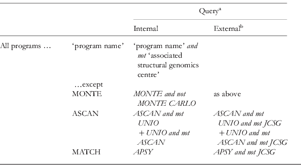
a A PDB ‘Advanced Search’ was performed with the listed queries as a ‘Text Search’ within all solution NMR depositions.
b Depositions for which the author list included one of the program authors were discarded.
PDB search strings for NOE assignment programs

a A PDB ‘Advanced Search’ was performed with the listed queries as a ‘Text Search’ within all solution NMR depositions.
b For external hits, the internal query was supplemented with ‘and not’ ‘associated structural genomics centre’; i.e. for CANDID this was ‘and not JCSG and not RIKEN’. Also, depositions were discarded for which one of the structure's authors was/is also involved in program development.
c CYANA is also used for simulated-annealing structure calculation, but not necessarily with CANDID. The number of CYANA hits (2460) overestimates the use of CANDID, but excluding all those that do not also reference other associated software (as was done here) is surely an underestimate.
PDB search strings for peak-picking algorithms
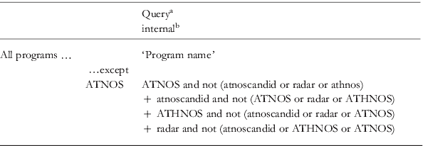
a A PDB ‘Advanced Search’ was performed with the listed queries as a ‘Text Search’ within all solution NMR depositions.
b For external hits, the internal query was supplemented with ‘and not’ ‘associated structural genomics centre’. Also, depositions were discarded for which one of the structure's authors was/is also involved in program development.
Search string for PDB entries for which some automation was used

a A PDB ‘Advanced Search’ was performed with the listed queries as a ‘Text Search’ within all solution NMR depositions.
PDB search strings for torsion-angle prediction programs

a A PDB ‘Advanced Search’ was performed with the listed queries as a ‘Text Search’ within all solution NMR depositions.