


1. Introduction
In astrophysical fluid bodies, such as metallic liquid cores and subsurface oceans, complex fluid flows can be excited by mechanical forcing (Le Bars, Cébron & Le Gal Reference Le Bars, Cébron and Le Gal2015). Libration, precession and tides, which correspond to harmonic perturbations of the rotation rate, rotation axis and body shape, respectively, are the most common large-scale forcings originating from gravitational interactions between orbiting bodies. Libration in particular is crucial for quasi-synchronised bodies locked in a spin–orbit resonance with their orbiting companion. The amplitude of the response to libration forcing helps constrain the internal structure of astrophysical bodies, indicating, for example, the existence of a subsurface ocean in Enceladus (Thomas et al. Reference Thomas, Tajeddine, Tiscareno, Burns, Joseph, Loredo, Helfenstein and Porco2016). The internal flows driven by such forcing have been extensively studied both numerically (Calkins et al. Reference Calkins, Noir, Eldredge and Aurnou2010; Cébron et al. Reference Cébron, Le Bars, Noir and Aurnou2012; Favier et al. Reference Favier, Grannan, Le Bars and Aurnou2015) and experimentally (Noir et al. Reference Noir, Hemmerlin, Wicht, Baca and Aurnou2009, Reference Noir, Cébron, Le Bars, Sauret and Aurnou2012; Grannan et al. Reference Grannan, Le Bars, Cébron and Aurnou2014; Le Reun, Favier & Le Bars Reference Le Reun, Favier and Le Bars2019).
In a rotating fluid, the Coriolis acceleration acts as a restoring force leading to the propagation of inertial waves whose frequency  $\omega ^*$ is smaller than twice the rotation rate
 $\varOmega ^*$ (Greenspan Reference Greenspan1968). In closed geometries, propagating inertial waves can eventually form global modes which can be resonantly excited by an external forcing (Aldridge & Toomre Reference Aldridge and Toomre1969). While analytical inviscid solutions exist for simple geometries such as the cylinder or the sphere, the ill posedness of the inviscid problem in a closed domain implies that singularities are the norm rather than the exception. Even when inviscid modes exist, such as for the cylinder, viscous corrections at the corners tend to spawn internal shear layers (McEwan Reference McEwan1970). In a spherical shell, two types of inviscid singularities are observed. Attractors are formed by the gradual convergence of characteristics along which inertial-wave beams propagate (Rieutord, Georgeot & Valdettaro Reference Rieutord, Georgeot and Valdettaro2001; Rieutord & Valdettaro Reference Rieutord and Valdettaro2018). A second type of singularity appears wherever the boundary is locally tangent to the direction of propagation of inertial waves, the so-called critical latitude (Kerswell Reference Kerswell1995). Viscosity naturally regularises these inviscid attractors and the singular surfaces associated with critical latitudes, which gives rise to different types of internal shear layers propagating in the bulk of the rotating fluid. These shear layers are also relevant to stratified fluids, which can support internal gravity waves that are very similar at the linear level with inertial waves in rotating fluids. Internal and inertial attractors have been experimentally found in a rectangular basin with one sloping boundary by Maas et al. (Reference Maas, Benielli, Sommeria and Lam1997) and Manders & Maas (Reference Manders and Maas2003), respectively. The internal shear layers spawned by critical latitudes on concave and convex boundaries have also been observed experimentally in a precessing spheroid (Noir et al. Reference Noir, Brito, Aldridge and Cardin2001) and librating (spherical and ellipsoidal) shells (Koch et al. Reference Koch, Harlander, Egbers and Hollerbach2013; Lemasquerier et al. Reference Lemasquerier, Grannan, Vidal, Cébron, Favier, Bars and Aurnou2017), respectively. They could play an important role in the mixing of stratified fluids (Brouzet et al. Reference Brouzet, Ermanyuk, Joubaud, Sibgatullin and Dauxois2016; Dauxois et al. Reference Dauxois, Joubaud, Odier and Venaille2018) and the generation of zonal flows in rapidly rotating fluid bodies (Maas Reference Maas2001; Morize et al. Reference Morize, Le Bars, Le Gal and Tilgner2010; Favier et al. Reference Favier, Barker, Baruteau and Ogilvie2014; Le Dizès Reference Le Dizès2015).
The dependence of oscillating internal shear layers on frequency has been tackled both as eigenvalue (Rieutord & Valdettaro Reference Rieutord and Valdettaro1997; Rieutord et al. Reference Rieutord, Georgeot and Valdettaro2001; Rieutord, Valdettaro & Georgeot Reference Rieutord, Valdettaro and Georgeot2002; Rieutord & Valdettaro Reference Rieutord and Valdettaro2018) and forced problems (Ogilvie Reference Ogilvie2009; Rieutord & Valdettaro Reference Rieutord and Valdettaro2010; Lin & Ogilvie Reference Lin and Ogilvie2018, Reference Lin and Ogilvie2021). Eigenmodes computed with the first approach are categorised as attractors, critical-latitude and quasi-regular modes based on the path of characteristics (Rieutord & Valdettaro Reference Rieutord and Valdettaro2018). For the forced problem, the response is classified as resonant, non-resonant or anti-resonant when its dissipation increases, remains constant or vanishes as viscosity tends to zero (Rieutord & Valdettaro Reference Rieutord and Valdettaro2010). The anti-resonant response occurs at the frequencies of periodic orbits. The non-resonant counterpart is observed at the frequencies of attractor modes, while the resonant one corresponds to the frequencies where global modes are hidden beneath the localised wave beams (Lin & Ogilvie Reference Lin and Ogilvie2021).
There are numerous theoretical and numerical studies investigating the scaling laws of oscillating internal shear layers. It is now accepted that the width of the shear layers spawned from the critical latitude scales like  $E^{1/3}$ (Walton Reference Walton1975b; Kerswell Reference Kerswell1995), where
 $E$ is the Ekman number measuring the importance of viscosity compared with rotational effects. Such a scaling has been demonstrated in several numerical works (Favier et al. Reference Favier, Barker, Baruteau and Ogilvie2014; Lin & Noir Reference Lin and Noir2021). However, the scaling for the amplitude of the response is disputed in the literature. Early theoretical predictions by Kerswell (Reference Kerswell1995) asserted that the strength of the internal shear layers spawned from the inner boundary in a spherical shell should follow a
 $E^{1/6}$ scaling, which is also observed numerically (Calkins et al. Reference Calkins, Noir, Eldredge and Aurnou2010; Favier et al. Reference Favier, Barker, Baruteau and Ogilvie2014; Cébron et al. Reference Cébron, Laguerre, Noir and Schaeffer2019). However, by asymptotically matching the solution of the internal shear layer to that of the boundary layer near the critical latitude, Le Dizès & Le Bars (Reference Le Dizès and Le Bars2017) found that the amplitude should scale with
 $E^{1/12}$. Recent numerical results by Lin & Noir (Reference Lin and Noir2021) at Ekman numbers in the range
 $10^{-7}< E<10^{-5}$, namely at lower viscosities than previous work, tend to favour the scaling
 $E^{1/12}$ over
 $E^{1/6}$. In the present paper, we will further validate the amplitude scaling
 $E^{1/12}$ by reaching Ekman numbers as low as
 $E=10^{-10}$.
One of the difficulties associated with these internal shear layers is their behaviour as they bounce on solid boundaries. Moore & Saffman (Reference Moore and Saffman1969) and Thomas & Stevenson (Reference Thomas and Stevenson1972) introduced self-similar solutions to describe the wave beams in unbounded geometries for rotating and stratified fluids, respectively. These similarity solutions are leading-order expressions describing the viscous smoothing in a  ${{O}}(E^{1/3})$ layer of a local inviscid singularity propagating along a characteristic line. Le Dizès & Le Bars (Reference Le Dizès and Le Bars2017) applied these solutions to the case of the critical-latitude singularity on a librating axisymmetric convex surface. They also numerically demonstrated the ability of the self-similar solutions to describe the internal shear layers generated by a librating spheroid in an unbounded domain. In a bounded domain, such as a spherical shell, where reflections on the boundaries and attractor singularities exist, the similarity solutions were found to be able to describe the internal shear layers created by the critical-latitude singularity (Walton Reference Walton1975a) and attractors (Rieutord et al. Reference Rieutord, Georgeot and Valdettaro2001; Ogilvie Reference Ogilvie2005). Internal shear layers are wave packets. How these wave packets are reflected on the boundaries depends on the geometry of the reflecting surfaces. On a flat surface, they are completely reflected, as plane waves, in a characteristic direction different from the incident one (Phillips Reference Phillips1963, Reference Phillips1966; Kistovich & Chashechkin Reference Kistovich and Chashechkin1994; Le Dizès Reference Le Dizès2020), while on a curved surface there may exist ‘back-reflected’ waves along the incident characteristic but in the opposite direction (Baines Reference Baines1971a). Moreover, when the incident characteristic is tangent to the curved surface at some point, the incident waves are also split into two different waves (Baines Reference Baines1971b). However, in both cases, if the wavelengths of the incident beam are sufficiently large compared with the length scales of the reflecting surface, the back-reflected response is negligible (Baines Reference Baines1971a). We shall be in this situation in the present study.
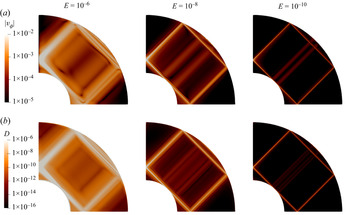
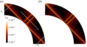
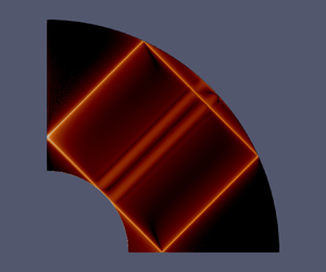
In this paper, we consider the inertial waves generated by the longitudinal libration of the inner core of a rotating spherical shell in the linear limit of infinitesimal forcing amplitudes and Ekman numbers. The objective is to generalise the work of Le Dizès & Le Bars (Reference Le Dizès and Le Bars2017) to the case of a closed geometry involving reflections on curved solid boundaries. For simplicity, we do not consider the case of attractors and focus on the shear layer spawned from the critical latitude at a particular frequency for which the characteristic path eventually comes back to the critical latitude after several reflections. These periodic orbits (Rieutord et al. Reference Rieutord, Georgeot and Valdettaro2001; Rieutord & Valdettaro Reference Rieutord and Valdettaro2018) are a natural choice since the path of characteristics remains topologically simple, which would not be the case for frequencies sustaining attractors. For illustration, the shear layers in a spherical shell forced by the libration of the inner core are displayed in figure 1. This solution is obtained by the direct numerical integration of the linearised viscous equations and will serve as a reference to which the generalised asymptotic solution introduced in this paper will be systematically compared.
Contours of the amplitude of azimuthal velocity  $|v_{\phi }|$ (a) and dissipation
 $D$ (b) for three Ekman numbers obtained by the direct numerical integration of the linear forced viscous problem. The aspect ratio of the spherical shell is
 $\eta =0.35$ and the dimensionless librating frequency of the inner core is
 $\omega =\sqrt {2}$.

The paper is organised as follows. Section 2.1 introduces the setting of the problem and the basic equations. Then we describe the asymptotic theory in § 2.2. The self-similar solution in an open geometry and its scaling are recalled in § 2.2.1. In § 2.2.2, we recall the reflection laws on a flat boundary and on the axis. The extended asymptotic solutions for different regions of the spherical shell are derived in §§ 2.2.3–2.2.4. Section 2.3 is devoted to the description of the numerical method used to integrate the linearised equations. The comparison between the theoretical predictions and the numerical results is performed in § 3 for the solution in the bulk. Close to the axis, the self-similar solution is singular. In § 4, a new asymptotic solution valid close to the axis is derived using Hankel transforms and compared with the numerical solution. Finally, a summary and possible directions for future works are discussed in § 5.
2. Framework
2.1. Basic equations
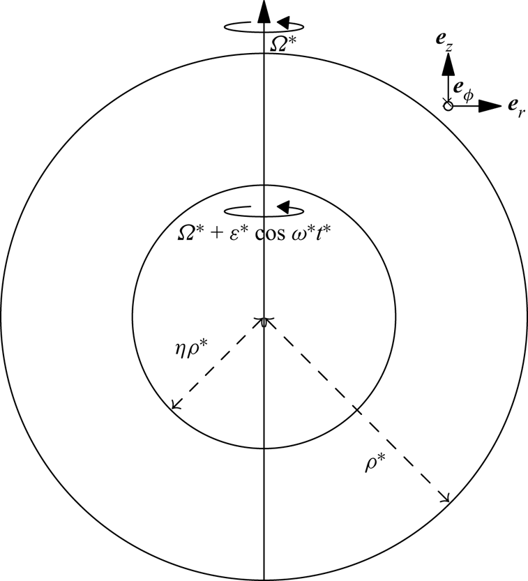
We consider the viscous incompressible rotating flow filling a spherical shell and forced by the libration of the inner core, as shown in figure 2. The radii of the outer and inner spheres are  $\rho ^*$ and
 $\eta \rho ^*$ (with
 $0<\eta <1$), respectively. The flow between them rotates around the symmetry axis
 $Oz$ and with an angular velocity
 $\varOmega ^*$ . The inner core librates at an amplitude
 $\varepsilon ^*$ and frequency
 $\omega ^*$, such that the corresponding angular rotation rate is
 $\varOmega ^*+\varepsilon ^*\cos (\omega ^*t^*)$. Space and time variables are non-dimensionalised by the outer radius
 $\rho ^*$ and angular period
 $1/\varOmega ^*$, respectively. The non-dimensional radii of the outer and inner shells are then
 $1$ and
 $\eta$, respectively, while the non-dimensional angular velocity of the inner core is
 $1+\varepsilon \cos \omega t$ with libration amplitude
 $\varepsilon =\varepsilon ^*/\varOmega ^*$ and libration frequency
 $\omega =\omega ^*/\varOmega ^*$. The Ekman number is defined by
 \begin{equation} E=\frac{\nu}{\varOmega^*\rho^{*2}}, \end{equation}
with  $\nu$ being the kinematic viscosity.
Schematic of the problem: the outer shell of radius  $\rho ^*$ rotates with an angular velocity
 $\varOmega ^*$, while the inner one of radius
 $\eta \rho ^*$ rotates at
 $\varOmega ^*+\varepsilon ^*\cos (\omega ^*t^*)$ with
 $\varepsilon ^*$ and
 $\omega ^*$ being the amplitude and frequency of the libration, respectively.

Since we are concerned with the harmonic linear response in the limit of small viscosity, both the libration amplitude and the Ekman number are assumed to be small. The libration frequency  $\omega$ is chosen in the inertial-wave range such that it can be written as
 $\omega =2\cos \theta _c$. The angle
 $\theta _c$ indicates the direction of propagation of the inertial waves with respect to the equatorial plane. It also corresponds to the inclination angle that internal shear layers make with respect to this plane. In order to form a simple closed circuit,
 $\theta _c$ is fixed to
 $45^{\circ }$. This means that the libration frequency
 $\omega$ is fixed to
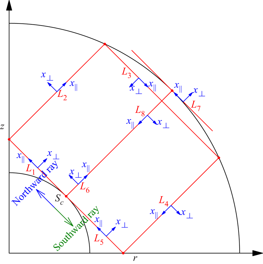
 $\sqrt {2}$. These values are unchanged throughout the paper. An example of the ray path is shown in figure 3, where the internal shear layer is initially spawned at the critical latitude
 $S_c$ and returns to it after bouncing on the axis, reflecting twice on the outer boundary and reflecting on the equatorial plane, thanks to the imposed symmetry.
Critical lines  $L_j$ (
 $j=1,2 \ldots 8$) and the local coordinate systems
 $(x_\parallel,x_\perp )$ for rays initially emitted in the northward direction. The opposite directions are used for rays initially emitted in the southward direction.

The flow is governed by the linearised incompressible Navier–Stokes equations in the rotating frame. We seek the following harmonic solution for the velocity  $\boldsymbol {V}$ and pressure
 $P$
 \begin{equation} (\boldsymbol{V}, P)=\varepsilon (\boldsymbol{v}, p)\, {\rm e}^{-\mathrm{i}\omega t}+{\rm c.c.} , \end{equation}
where the notation  ${\rm c.c.}$ denotes complex conjugate terms. The velocity
 $\boldsymbol {v}$ and pressure
 $p$ satisfy the following equations in the rotating frame
 $$\begin{gather} -\mathrm{i}\omega \boldsymbol{v}+2\boldsymbol{e}_z\times\boldsymbol{v} ={-}\boldsymbol{\nabla} p+E\nabla^2\boldsymbol{v} , \end{gather}$$
 $$\begin{gather}\boldsymbol{\nabla}\boldsymbol{\cdot}\boldsymbol{v}= 0 , \end{gather}$$
with the boundary conditions
 $$\begin{gather} \boldsymbol{v}=r\boldsymbol{e}_\phi \quad \text{on the inner shell,} \end{gather}$$
 $$\begin{gather}\boldsymbol{v}=\boldsymbol{0} \quad \text{on the outer shell,} \end{gather}$$
where  $r$ is the distance to the rotation axis.
2.2. Asymptotic theory
The asymptotic analysis is conducted within the cylindrical coordinate system  $(r,z,\phi )$. The basic idea of the asymptotic theory is to assume that the main features of the solution come from the propagation of the critical-latitude singularity
 $S_c$ localised at
 $r=\eta \sqrt {1-\omega ^2/4}$ and
 $z=\eta \omega /2$ on the inner sphere. For the frequency
 $\omega = \sqrt {2}$, this singularity is expected to propagate along the critical characteristic lines
 $L_j$ (
 $j=1 \dots 8$) and form a closed circuit (see figure 3). The northward rays correspond to the rays initially propagating along the line
 $L_1$. They then cover the circuit
 $L_1 \rightarrow L_2 \rightarrow L_3 \rightarrow L_4 \rightarrow L_5$, possibly bounce on the inner core leading to the additional path
 $L_6 \rightarrow L_7 \rightarrow L_8$ before starting the circuit again. Similarly, the southward rays start propagating on the line
 $L_5$ from
 $S_c$, travelling on
 $L_5 \rightarrow L_4 \rightarrow L_3\rightarrow L_2 \rightarrow L_1$ (possibly on
 $L_8\rightarrow L_7 \rightarrow L_6$) and continuing the same circuit again. The critical lines
 $L_1\text{--}L_5$ correspond to the main beam (inclined quadrilateral) observed in figure 1, while
 $L_6\text{--}L_8$ are responsible for the two secondary wider and weaker beams near the centre line
 $z=r$. Both northward and southward rays are expected to contribute to the solution. Note, however, that computing their contribution will require considering their interaction with the rotation axis and their reflections on boundaries.
For building the asymptotic solution around these critical lines, it is useful to introduce a local frame  $(x_\parallel,x_\perp )$ for each critical line where
 $x_\perp =0$ corresponds to the critical line itself. The variable
 $x_\parallel$ measures the travelled distance from the source along the critical lines. It increases as the ray propagates on each critical line. However, as we shall see below, it may exhibit a jump when the ray is reflected. The variable
 $x_\perp$ indicates the position with respect to the critical line. The orientation of
 $x_\perp$ can a priori be arbitrarily chosen. For convenience, we have assumed that the orientation does not change sign during the propagation, that is a ray at a positive
 $x_\perp$ stays at a positive
 $x_\perp$ after reflection. The orientation of the local frames shown in figure 3 is for the northward rays. Opposite local frames are taken for the southward rays.
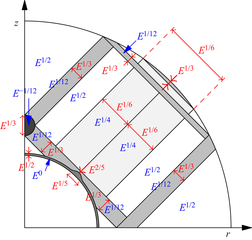
The final result of the asymptotic analysis in terms of Ekman scalings is summarised in figure 4. The Ekman layer adjacent to the inner core is characterised by a  $E^{1/2}$ width and a
 $E^{0}$ velocity amplitude. Around the critical latitude the width increases to
 $E^{2/5}$ with an extension of
 $E^{1/5}$ along the boundary (Roberts & Stewartson Reference Roberts and Stewartson1963). The width and the amplitude of the main beams around the critical lines
 $L_1\text{--}L_5$ are of order
 $E^{1/3}$ and
 $E^{1/12}$, respectively (see § 2.2.3), while those of the secondary beams around
 $L_6$ and
 $L_8$ are of order
 $E^{1/6}$ and
 $E^{1/4}$, respectively (see § 2.2.4). Near
 $L_7$, the beam recovers the
 $E^{1/3}$ width of the main beam, while it travels a distance of order
 $E^{1/6}$ along
 $L_7$. Around the axis where two main beams intersect, the length scale remains as
 $E^{1/3}$, while the amplitude diverges as
 $E^{-1/12}$ (see § 4).
Ekman scalings in a spherical shell: length scales and amplitudes are shown in red and blue, respectively.

2.2.1. Self-similar solution and scaling
As first shown by Moore & Saffman (Reference Moore and Saffman1969), the propagation and viscous smoothing of a localised singularity can be described in the limit of small Ekman numbers by a self-similar solution. This result has been used and applied to the critical-latitude singularity generated by the libration of a sphere in Le Dizès & Le Bars (Reference Le Dizès and Le Bars2017). We now briefly recall the main results.
The self-similar form is derived by considering the small Ekman number limit of the governing equations projected onto the local frame  $(x_\parallel,x_\perp )$. The solution is characterised by
 $v_\parallel$,
 $v_\perp$,
 $v_\phi$ and
 $p$. The former two are velocity components along and perpendicular to the critical lines, while the latter two correspond to the azimuthal velocity and pressure, respectively. As the width of the internal shear layer regularised by viscosity scales with
 $E^{1/3}$, all quantities are expanded with the perturbation parameter
 $E^{1/3}$. The dependence on the radial coordinate
 $r$ is removed by dividing the solution by
 $\sqrt {r}$. At leading order, only
 $v_\parallel$ and
 $v_\phi$ are required to fully describe the solution. The former has the following self-similar form:
 \begin{equation} v_\parallel{=}\frac{1}{\sqrt{r}}C_0H_m(x_\parallel,\zeta)= \frac{1}{\sqrt{r}}C_0\left(\frac{x_\parallel}{2\sin\theta_c} \right)^{{-}m/3}h_m(\zeta), \end{equation}
with the similarity variable
 \begin{equation} \zeta=x_\perp E^{{-}1/3}\left(\frac{2\sin\theta_c}{x_\parallel}\right)^{1/3}, \end{equation}
and the function
 \begin{equation} h_m(\zeta)=\frac{{\rm e}^{-\mathrm{i}m{\rm \pi}/2}}{(m-1)!}\int^{+\infty}_{0}\, {\rm e}^{\mathrm{i}p\zeta-p^3}p^{m-1}\, {\rm d} p . \end{equation}
The real index  $m$ and the complex amplitude
 $C_0$ are the parameters characterising the strength and the (complex) amplitude of the singularity. Expression (2.5) is a leading-order expression of a viscous solution in the limit of small Ekman numbers. Next-order corrections are expected to be
 ${{O}}(E^{1/3})$. The solution preserves the self-similar structure described by
 $h_m(\zeta )$ during its propagation and decay as
 $x_\parallel ^{-m/3}$ with
 $x_\parallel$ being the distance from the source. Note that there are two singularities in (2.5). One is on the rotation axis where
 $r=0$, the other is at the source
 $x_\parallel =0$. The similarity solution requires modification close to these two regions. In addition, it is modified close to the boundaries where the solution should be derived following the more classical
 $E^{1/2}$ scaling characteristic of Ekman viscous layers (see Le Dizès Reference Le Dizès2020).
Le Dizès & Le Bars (Reference Le Dizès and Le Bars2017) derived the particular values of the two parameters  $m$ and
 $C_0$ for any axisymmetric convex librating object by matching the similarity solution with the boundary layer solution close to the critical latitude. As a necessary condition for matching, they obtained the particular values
 \begin{equation} m=5/4, \end{equation}
and
 $$\begin{gather} C_0= \frac{E^{1/12}}{8(2\sin\theta_c)^{3/4}}\, {\rm e}^{\mathrm{i}{\rm \pi}/2} \quad \text{for a northward ray}, \end{gather}$$
 $$\begin{gather}C_0= \frac{E^{1/12}}{8(2\sin\theta_c)^{3/4}}\, {\rm e}^{\mathrm{i}3{\rm \pi}/4} \quad \text{for a southward ray}. \end{gather}$$
The curvature at the critical latitude  $\kappa _c=-\sin {\theta _c}$ for the spherical inner core has been applied. Note that there is an error concerning the phase of
 $C_0$ in Le Dizès & Le Bars (Reference Le Dizès and Le Bars2017), which is corrected here. The value
 $m=5/4$ implies that the ray amplitude decays as
 $x_\parallel ^{-5/12}$. The parameters
 $C_0$ for the northward and southward rays only differ by a phase shift of
 ${\rm \pi} /4$. These two values of
 $C_0$ only hold for the initial rays directly spawned from the source. For the subsequent reflected rays, the phase and amplitude of
 $C_0$ have to be modified as they will be in the next subsection.
The relation between the azimuthal velocity  $v_\phi$ and the parallel velocity
 $v_\parallel$ is
 \begin{equation} v_\phi={\pm}\mathrm{i}v_\parallel. \end{equation}
The sign depends on the angle between the local unit vector  $\boldsymbol {e}_\parallel$ and the global unit vector
 $\boldsymbol {e}_r$. The
 $+$ sign is taken for obtuse angles, while the
 $-$ sign is taken for acute ones.
The values (2.9a,b) of  $C_0$ clearly show that the amplitude of the leading-order asymptotic solution scales with
 $E^{1/12}$. Numerical results in open and closed geometries have partially confirmed such scaling at relatively high Ekman numbers (above
 $10^{-7}$) (Le Dizès & Le Bars Reference Le Dizès and Le Bars2017; Lin & Noir Reference Lin and Noir2021). Further evidence about this scaling at lower Ekman numbers will be provided here.
2.2.2. Reflections on the outer boundary and on the axis
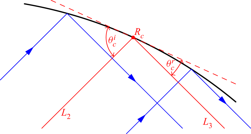
As shown in figure 3, there are two reflections ( $L_2\rightarrow L_3$ and
 $L_3\rightarrow L_4$) on the outer boundary. How the incident beam reflects on the curved boundary depends on its relative length scales compared with those of the reflecting surface. As proved by Baines (Reference Baines1971a) for a plane wave, the ‘back-reflected’ wave along the incident characteristic but in the opposite direction vanishes when the incident wavenumber becomes large, and the incident wave feels the curved boundary as locally flat and reflects as a local plane wave on a flat surface. For our case, the wave beam described by the similarity solution (2.5) is shown to be dominated by large wavenumbers (see Appendix A). Therefore, the possible ‘back-reflected’ wave beam is negligible and not considered, as shown in the figure 5 for the reflection of an incident beam along
 $L_2$ yielding only a reflected beam along
 $L_3$. Moreover, the reflection on the curved boundary can be approximated by that on the flat tangent surface at the critical reflection point
 $R_c$ (in red dashed line).
Reflection on the outer boundary from the incident beam around  $L_2$ to the reflected beam around
 $L_3$: red and blue solid lines are critical lines and wave beams, respectively; the red dashed line is the tangent plane at the reflection point
 $R_c$;
 $\theta ^i_c$ and
 $\theta ^r_c$ are the incident and reflected angles.

The reflection of internal shear layers on a flat boundary has been studied by Le Dizès (Reference Le Dizès2020). The incident and reflected wave beams were found to preserve, at leading order, their self-similar structures, which are
 \begin{equation} v_\parallel^i=C_0^i H_m(x_\parallel^i,\zeta^i)/\sqrt{r}, \quad v_\parallel^r=C_0^r H_m(x_\parallel^r,\zeta^r)/\sqrt{r}, \end{equation}
where the superscripts  $i$ and
 $r$ denote the variables associated with the incident and reflected beams, respectively. The corresponding reflection laws take the forms
 \begin{equation} \frac{x_{{\parallel} c}^i}{x_{{\parallel} c}^r}=K^3,\quad \frac{C_0^i}{C_0^r}=K^{m-1}, \end{equation}
with  $K=\sin \theta ^i_c/\sin \theta ^r_c$ the ratio of the sines of the critical incident and reflected inclination angles
 $\theta ^i_c$ and
 $\theta ^r_c$. Here,
 $x_{\parallel c}^i$ and
 $x_{\parallel c}^r$ are the distances between the critical reflection point
 $R_c$ and the source before and after the reflection, respectively. The above reflection laws suggest that the effective source is displaced and the amplitude is modified by the reflection on the flat boundary. The reflected beam appears to be generated from a ‘virtual’ source located at the position
 $x_\parallel ^r$ away from the reflection point
 $R_c$ and with a strength
 $C_0^r$. Note that
 $K$ is a real number, so the phase is left unchanged by the reflection on the boundary. It is worth mentioning that viscous corrections are also created during the reflection process. These corrections are not considered in the present work. Le Dizès (Reference Le Dizès2020) has shown that they are
 ${{O}}(E^{1/6})$ smaller and also possess a self-similar structure.
The reflection on the axis from  $L_1$ to
 $L_2$ (see figure 3) has been discussed by Le Dizès & Le Bars (Reference Le Dizès and Le Bars2017) and Rieutord & Valdettaro (Reference Rieutord and Valdettaro2018), which reveals that the phase of the parallel velocity is shifted by
 ${\rm \pi} /2$ while the amplitude and the distance to the source is kept the same. By the same method, the reverse reflection from
 $L_2$ to
 $L_1$ also shifts the phase of the parallel velocity by
 ${\rm \pi} /2$ while keeping all other quantities unchanged. In other words, we always have on the axis
 \begin{equation} C_0^{r}={\rm e}^{\mathrm{i}{\rm \pi}/2}C_0^{i}. \end{equation}
2.2.3. Asymptotic solution for the main beams around the critical lines  $L_1\text{--}L_5$

The similarity solution (2.5) and the reflection laws ((2.12) and (2.13)) are applied to build the asymptotic solutions around the critical lines  $L_1\text{--}L_5$ for the two beams shown in figure 3. Taking the northward beam travelling from
 $L_1$ to
 $L_5$ as an example, the two ratios of sines of inclination angles at the points
 $R_1$ and
 $R_2$ shown in figure 3 take the forms
 \begin{equation} K_1=\sqrt{1-\eta^2}/\eta,\quad K_2=1/K_1. \end{equation}
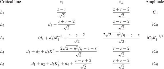
The lengths of the critical lines  $L_1\text{--}L_5$ in figure 3 take the values
 \begin{align} d_1=\sqrt{2},\quad d_2=\sqrt{2}\left({-}1+\frac{\sqrt{2-\eta^2}}{\eta}\right), \quad d_3=2\sqrt{2}, \quad d_4=d_2, \quad d_5=d_1, \end{align}
rescaled by the distance to the axis of the critical latitude in accordance with the non-dimensionalisation adopted by the asymptotic theory (Le Dizès & Le Bars Reference Le Dizès and Le Bars2017). The global coordinates  $(r,z)$ of a point
 $P$ are transformed into the local coordinates
 $(x_\parallel, x_\perp )$ for every critical line by computing the distances to the source
 $S_c$ and to the corresponding critical line, respectively. The travelled distance
 $x_\parallel$ should be modified on the boundary according to (2.12a), and the amplitude
 $C_0$ should be modified on the boundary and axis according to (2.12b) and (2.13), respectively. We obtain for the northward beam the characteristics given in table 1. For the southward beam travelling from
 $L_5$ to
 $L_1$, the multiplicative inverses of the ratios (2.14) are taken, and the local coordinates and amplitudes for every critical line can be constructed similarly.
Characteristics of the northward beam from  $L_1$ to
 $L_5$.

Up to this stage, we have described how to build the asymptotic solution along one complete revolution of the periodic orbit, from the critical latitude and back. However, it is natural to assume that the self-similar solution will continue propagating along the periodic characteristic path until its amplitude eventually becomes negligible. When the northward beam goes back to the critical latitude on the inner core, the outer part of the beam ( $x_\perp >0$) is expected to propagate forward for another cycle without being modified by the inner core. By contrast, the inner part (
 $x_\perp <0$) is expected to reflect on the inner core and follow another path on
 $L_6\text{--}L_8$ before starting a new cycle. We shall see in § 2.2.4 that this different circuit has actually no impact on the beam: its new expression on
 $L_1$ is the same as if the inner core was not present. For this reason, the whole beam can be assumed to propagate forward for another cycle without considering the presence of the inner core. The same is naturally true for the southward beam. For each cycle, the self-similar nature of the local solution should be preserved since only
 $C_0$ and
 $x_\parallel$ are modified by reflections on the axis and boundaries. The asymptotic solution for the
 $n$th cycle can be expressed as
 \begin{equation} \sqrt{r}v_{{\parallel} n}=C_{n}H_m(x_{{\parallel} n},\zeta_{n}). \end{equation}
The subscript  $n$ indicates a variable associated with the
 $n$th cycle. When
 $n=0$, (2.16) is equivalent to (2.5) for the very first cycle. The variables of the subsequent cycles are related to those of the first
 $n=0$ cycle by
 $$\begin{gather} x_{{\parallel} n} = x_{{\parallel} 0}+nL, \end{gather}$$
 $$\begin{gather}\zeta_{n} =\zeta_{0}(x_{{\parallel} n}/x_{{\parallel} 0})^{1/3}, \end{gather}$$
 $$\begin{gather}C_{n}=C_{0}\, {\rm e}^{\mathrm{i}n{\rm \pi}/2}, \end{gather}$$
where  $L$ is the travelled distance within one cycle, and
 ${\rm \pi} /2$ is the phase shift induced by the reflection on the axis occurring once per cycle. Here,
 $L$ takes the following formulas for different critical lines
 $$\begin{gather} L=d_1+d_2+d_3K_1^3+d_4+d_5, \quad \text{for} \quad L_1, L_2, L_4, L_5, \end{gather}$$
 $$\begin{gather}L=(d_1+d_2+d_4+d_5)K_1^{{-}3}+d_3, \quad \text{for} \quad L_3. \end{gather}$$
Note that  $L$ does not change from one cycle to another and is the same for both beams. For the reflection
 $L_2\leftrightarrow L_3$,
 $L$ and
 $x_{\parallel 0}$ are discontinuous (see table 1 and (2.20a,b)), while
 $L/x_{\parallel 0}$ is continuous. The same is also true for the reflection
 $L_3\leftrightarrow L_4$. Note also that the norm of the amplitude of the self-similar solution does not change after each cycle (
 $|C_n| = |C_0|$). This is associated with the symmetric character of each cycle, which guarantees that the phases of contraction and expansion experienced by the beam during one cycle exactly compensate.
The complete asymptotic solution associated with one beam is thus the sum of the solution (2.16) for every cycle. After  $N+1$ cycles, we obtain
 \begin{equation} \sqrt{r}v_{{\parallel}}^{(N)}=\sum_{n=0}^N C_{n}H_m(x_{{\parallel} n},\zeta_{n}). \end{equation}
The self-similar solution decays with the travelled distance as  $x_\parallel ^{-5/12}$ (see (2.5) and (2.8)). This gives a behaviour in
 $n^{-5/12}$ of the coefficients of the series (2.21) that does not guarantee its absolute convergence. However, because
 $C_n$ is oscillating with
 $n$ (see (2.19)), the series does converge. The number of cycles can therefore be chosen as large as wanted. Using the relations ((2.17)–(2.19)), the series of the integrals (2.21) can be transformed to an integral of a geometric series
 \begin{equation} \sqrt{r}v_{{\parallel}}^{(N)}=C_{0}\left(\frac{x_{{\parallel} 0}}{2\sin\theta_c}\right)^{{-}m/3}\frac{{\rm e}^{-\mathrm{i}m{\rm \pi}/2}}{(m-1)!}\int^\infty_0\, {\rm e}^{\mathrm{i}p\zeta_0-p^3}p^{m-1}\sum_{n=0}^N \mathrm{i}^n\, {\rm e}^{{-}np^3L/x_{{\parallel} 0}}\, {\rm d} p. \end{equation}
Moreover, with the closed form of the geometric series the solution can be expressed by two parts
 \begin{equation} \sqrt{r}v_{{\parallel}}^{(N)}=C_{0}G_m(x_{{\parallel} 0},x_\perp, L)+\varepsilon_m^{(N)}(x_{{\parallel} 0},x_\perp, L), \end{equation}
with
 $$\begin{gather} G_m(x_{{\parallel} 0},x_\perp, L)=\left(\frac{x_{{\parallel} 0}}{2\sin\theta_c}\right)^{{-}m/3}g_m(\zeta_0, L/x_{{\parallel} 0}), \end{gather}$$
 $$\begin{gather}g_m(\zeta_0, L/x_{{\parallel} 0})=\frac{{\rm e}^{-\mathrm{i}m{\rm \pi}/2}}{(m-1)!}\int^\infty_0 \frac{{\rm e}^{\mathrm{i}p\zeta_0-p^3}p^{m-1}}{1-\mathrm{i}\, {\rm e}^{{-}p^3L/x_{{\parallel} 0}}}\, {\rm d} p, \end{gather}$$
and
 \begin{equation} \varepsilon_m^{(N)}=C_0\left(\frac{x_{{\parallel} 0}}{2\sin\theta_c}\right)^{{-}m/3}\frac{{\rm e}^{-\mathrm{i}m{\rm \pi}/2}}{(m-1)!} \int^\infty_0\, {\rm e}^{\mathrm{i}p\zeta_0-p^3}p^{m-1}\frac{-\mathrm{i}^{N+1}\, {\rm e}^{{-}p^3L(N+1)/x_{{\parallel} 0}}}{1-\mathrm{i}\, {\rm e}^{{-}p^3L/x_{{\parallel} 0}}}\, {\rm d} p. \end{equation}
The correction term  $\varepsilon _m^{(N)}$ behaves as
 \begin{equation} \varepsilon_m^{(N)} \sim{-}C_0\frac{{\rm e}^{-\mathrm{i}m{\rm \pi}/2}}{(m-1)!}\frac{1}{3}\left(\frac{2\sin\theta_c}{L}\right)^{m/3}\frac{\varGamma (m/3)}{1-\mathrm{i}}\mathrm{i}^{N+1}N^{{-}m/3}, \end{equation}
as the number of cycles becomes large. It vanishes as the number of cycles tends to infinity. Therefore, in the limit  $N\rightarrow \infty$, the asymptotic solution takes the form
 \begin{equation} \sqrt{r}v_{{\parallel}}=C_{0}G_m(x_\parallel,x_\perp, L). \end{equation}
Only the local coordinates in the very first cycle are needed to compute the asymptotic solution. Without any ambiguity, the subscript  $0$ denoting the very first cycle has been dropped for the parallel coordinate and similarity variable hereafter. The above discussion holds both for northward and southward rays. The final global asymptotic solution in the closed geometry is the sum of the solutions of both rays, that is
 \begin{equation} \sqrt{r}v_{{\parallel}}=C_0^{NW}G_m (x_\parallel^{NW},x_\perp^{NW},L)+C_0^{SW}G_m (x_\parallel^{SW},x_\perp^{SW},L), \end{equation}
where the superscripts  $NW$ and
 $SW$ denote northward and southward rays, respectively. Equation (2.28) provides the description of the parallel velocity, while the azimuthal velocity
 $v_\phi$ can be derived from the phase relation (2.10).
2.2.4. Asymptotic solution for the secondary beams around $L_6$ and $L_8$


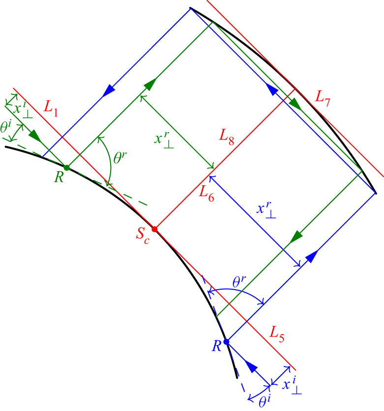
When the northward and southward beams come back to the critical latitude on the inner core, their corresponding critical lines become  $L_5$ and
 $L_1$, respectively (see figure 6). Because these two critical lines are tangent to the surface, the part of the beams below
 $L_5$ and
 $L_1$ reflects on the inner boundary, while the other part goes straight. This particular reflection is referred to as diffraction by Baines (Reference Baines1971b) for a plane wave. The reflected beams are then along
 $L_6\rightarrow L_7 \rightarrow L_8$ or
 $L_8 \rightarrow L_7\rightarrow L_6$ for the northward or southward beams, respectively (see solid blue and green lines in figure 6). These reflected beams correspond to the two secondary weaker beams near the line
 $z=r$ observed in figure 1. In order to construct the corresponding asymptotic solution, curvature effects for the reflection on the inner core must be included. For this purpose, the non-penetrability condition is applied at the reflection point
 $R$ (see figure 6) other than the critical one
 $S_c$, namely
 \begin{equation} \sin\theta^rv_\parallel^r\sim\sin\theta^iv_\parallel^i, \end{equation}
where  $\theta ^i$ and
 $\theta ^r$ are incident and reflected inclination angles at the reflection point
 $R$, respectively. Note that their values are different from the critical values at the critical reflection point
 $S_c$ due to the effect of curvature. The incident parallel velocity
 $v_\parallel ^i$ is obtained by propagating the similarity solution from the critical latitude back to it along
 $L_1\rightarrow L_2 \rightarrow L_3 \rightarrow L_4 \rightarrow L_5$ or the inverse sequence for the northward or southward beam, respectively, which is
 \begin{equation} v_\parallel^i=\frac{1}{\sqrt{r}}C_0\mathrm{i}\frac{{\rm e}^{-\mathrm{i}m{\rm \pi}/2}}{(m-1)!}\int^{\infty}_0\, {\rm e}^{\mathrm{i}px_\perp^{i}/E^{1/3}}\, {\rm e}^{{-}p^3L/(2\sin\theta_c)}p^{m-1}\, {\rm d} p \end{equation}
in terms of the local coordinates  $(x_\parallel ^i,x_\perp ^i)$. Note that
 $x_\parallel ^i=L$ has been applied. Taking the northward beam as an example, according to the geometry shown in figure 6,
 $x_\perp ^i$ and
 $x_\perp ^r$ can be expressed as a function of
 $\theta ^i$ as
 \begin{equation} x_\perp^i=\sqrt{2}\cos\theta^i-\sqrt{2},\quad x_\perp^r={-}\sqrt{2}\sin\theta^i. \end{equation}
Note that the coordinates are also calculated with reference to the distance to the axis of the critical latitude by which the radius of the inner core is  $\sqrt {2}$ (Le Dizès & Le Bars Reference Le Dizès and Le Bars2017). Moreover,
 $x_\perp ^i$ can be expressed in terms of
 $x_\perp ^r$ as
 \begin{equation} x_\perp^i=\sqrt{2-(x_\perp^r)^2}-\sqrt{2}. \end{equation}
The variable  $x_\perp ^r$ being small within the beam, we obtain the following relation at the leading order:
 \begin{equation} x_\perp^i\sim \lambda(x_\perp^r)^2, \end{equation}
where  $\lambda =\pm \sqrt {2}/4$. The minus and plus signs are for northward and southward beams, respectively. The inclination angles can also be expressed using
 $x_\perp ^r$ as
 \begin{equation} \sin\theta^i=\left|\frac{x_\perp^r}{\sqrt{2}}\right|,\quad \sin\theta^r=\sqrt{1-\left(\frac{x_\perp^r}{\sqrt{2}}\right)^2}\sim 1. \end{equation}
Therefore, the parallel velocity of the reflected beam takes the following form:
 \begin{equation} v_\parallel^r\sim \left|\frac{x_\perp^r}{\sqrt{2}}\right| \frac{1}{\sqrt{r}}C_0\mathrm{i}\frac{{\rm e}^{-\mathrm{i}m{\rm \pi}/2}}{(m-1)!} \int^{\infty}_0\, {\rm e}^{\mathrm{i}p\lambda (x_\perp^{r})^2/E^{1/3}}\, {\rm e}^{{-}p^3L/(2\sin\theta_c)}p^{m-1}\, {\rm d} p. \end{equation}
The phase is proportional to  $(x_\perp ^{r})^2/E^{1/3}$, which means that
 $x_\perp ^r$ scales with
 $E^{1/6}$. The reflected beam is therefore expected to be wider than the self-similar solution with a width of order
 $E^{1/6}$. Because of this larger transverse scale, it should not be affected by viscous diffusion within the shell. In other words, expression (2.35) for
 $v_\parallel ^r$ is expected to remain valid on the whole segment
 $L_6$ (respectively
 $L_8$) for the northward beam (respectively for the southward beam). Each beam is then reflected twice on the outer boundary (see figure 6). Between these two reflection points on
 $L_7$, the beam recovers its initial width but because it travels a distance of order
 $E^{1/6}$, the viscous diffusion is still negligible. Moreover, the reflections on the outer boundary are perfectly symmetric, such that the northward and southward beams remain unchanged after these two reflections. The formula (2.35) then still holds for the northward or southward beam around
 $L_8$ or
 $L_6$, respectively. Namely, for each beam, the asymptotic solution (after rescaling with
 $1/\sqrt {r}$) is anti-symmetric about the centre line
 $z=r$.
Schematic of the reflection on the inner boundary and the resulting rays around  $L_6\text{--}L_8$. Blue and green lines are northward and southward rays; red lines are critical lines.

Note that, contrary to the solution around the main beam  $L_1\text{--}L_5$, the asymptotic solution (2.35) for
 $L_6$ and
 $L_8$ is no longer self-similar.
The asymptotic solution (2.35) corresponds to the first cycle only. The summation strategy used in the § 2.2.3 for  $L_1\text{--}L_5$ can also be applied to construct the asymptotic solution around
 $L_6$ and
 $L_8$ after an infinite number of cycles. The parallel velocity for the
 $n^{th}$ cycle is
 \begin{equation} v_\parallel^{(n)}\sim\left|\frac{x_\perp}{\sqrt{2}}\right| \frac{1}{\sqrt{r}}C_0\mathrm{i}^n\frac{{\rm e}^{-\mathrm{i}m{\rm \pi}/2}}{(m-1)!}\int^{\infty}_0\, {\rm e}^{\mathrm{i}p\lambda (x_\perp)^2/E^{1/3}}\, {\rm e}^{{-}p^3(nL)/(2\sin\theta_c)}p^{m-1}\, {\rm d} p, \end{equation}
with the phase shift equal to  $\mathrm {i}^n$ and the travelled distance equal to
 $nL$. The summation of the above formula from
 $n=1$ to
 $\infty$ yields the asymptotic solution after an infinite number of cycles
 \begin{equation} v_\parallel{\sim}\left|\frac{x_\perp}{\sqrt{2}}\right| \frac{1}{\sqrt{r}}C_0\frac{{\rm e}^{-\mathrm{i}m{\rm \pi}/2}}{(m-1)!}\int^{\infty}_0\, {\rm e}^{\mathrm{i}p\lambda (x_\perp)^2/E^{1/3}}\frac{\mathrm{i}\, {\rm e}^{{-}p^3L/(2\sin\theta_c)}}{1-\mathrm{i}\, {\rm e}^{{-}p^3L/(2\sin\theta_c)}}p^{m-1}\, {\rm d} p. \end{equation}
This formula holds for both northward and southward rays. The final solution is the sum of both solutions.
Finally, it is worth mentioning that, because  $x_\perp$ is
 $O(E^{1/6})$ along
 $L_6$ and
 $L_8$ and
 $C_0$ is
 $O(E^{1/12})$, the amplitude of
 $v_\parallel$ is smaller than on the other lines and exhibits a new scaling in
 $E^{1/4}$.
2.3. Numerical method
In order to validate the asymptotic approach, we now consider the complete numerical solution of the linear viscous harmonic problem described in § 2.1. The governing equations (2.3) are solved numerically in spherical coordinates  $(\rho,\vartheta,\phi )$, where
 $\rho$,
 $\vartheta$ and
 $\phi$ are the radial distance from the centre of the sphere, polar and azimuthal angles, respectively. In order to compare the numerical results with asymptotic predictions obtained within a different cylindrical coordinate system, the azimuthal velocity is adopted since this velocity component is the same in both cylindrical and spherical frames.
As in Rieutord & Valdettaro (Reference Rieutord and Valdettaro1997), the fields are expanded onto spherical harmonics in the polar and azimuthal directions and onto Chebyshev polynomials in the radial direction. We consider the expansion
 \begin{equation} \boldsymbol{v}=\sum_{l=0}^{+\infty}\sum_{m={-}l}^{{+}l}u_m^l(\rho) \boldsymbol{R}_l^m+v_m^l(\rho)\boldsymbol{S}_l^m+w_m^l(\rho)\boldsymbol{T}_l^m, \end{equation}
with
 \begin{equation} \boldsymbol{R}_l^m=Y_l^m(\vartheta,\varphi)\boldsymbol{e}_\rho, \quad \boldsymbol{S}_l^m=\boldsymbol{\nabla}{Y}_l^m, \quad \boldsymbol{T}_l^m=\boldsymbol{\nabla}\times\boldsymbol{R}_l^m, \end{equation}
where gradients are taken on the unit sphere. Projecting the curl of the momentum equation (2.3a) onto this basis yields (Rieutord Reference Rieutord1987)
 \begin{align} \left. \begin{array}{l} \displaystyle E\varDelta_lw^l+\mathrm{i}\omega w^l={-}A_l\rho^{l-1} \dfrac{\partial}{\partial \rho}\left(\dfrac{u^{l-1}}{\rho^{l-2}} \right)-A_{l+1}\rho^{{-}l-2}\dfrac{\partial}{\partial \rho}(\rho^{l+3}u^{l+1}) ,\\ \displaystyle E\varDelta_l\varDelta_l(\rho u^l)+\mathrm{i}\omega \varDelta_l(\rho u^l)=B_l\rho^{l-1}\dfrac{\partial}{\partial \rho} \left(\dfrac{w^{l-1}}{\rho^{l-1}}\right)+B_{l+1}\rho^{{-}l-2} \dfrac{\partial}{\partial \rho}(\rho^{l+2}w^{l+1}), \end{array} \right\}, \end{align}
with
 \begin{equation} A_l=\frac{1}{l\sqrt{4l^2-1}}, \quad B_l=l^2(l^2-1)A_l, \quad \varDelta_l=\frac{{\rm d}^2}{{\rm d} \rho^2} + \frac{2}{\rho}\frac{{\rm d}}{{\rm d} \rho} -\frac{l(l+1)}{\rho^2}. \end{equation}
Axisymmetry ( $m=0$) is assumed. The unknown variables in (2.40) are only
 $w^l$ and
 $u^l$. The third component
 $v^l$ is related to
 $u^l$ through the continuity equation (2.3b), that is
 \begin{equation} v^l=\frac{1}{\rho l(l+1)}\frac{{\rm d} \rho^2u^l}{{\rm d} \rho}. \end{equation}
The no-slip boundary conditions on the outer core impose that
 \begin{equation} w^l=u^l=\frac{{\rm d} u^l}{{\rm d} \rho}=0, \text{ at } \rho=1. \end{equation}
The libration on the inner boundary imposes a forcing in the azimuthal direction. Its projection onto spherical harmonics yields the inhomogeneous boundary conditions on the inner core
 \begin{equation} w^l=2\sqrt{\frac{\rm \pi}{3}}\eta\delta_{1,l} , \quad u^l=\frac{{\rm d} u^l}{{\rm d} \rho}=0 \text{ at } \rho=\eta , \end{equation}
where  $\delta _{i,j}$ is the Kronecker symbol.
Equations ((2.40)–(2.44)) are then discretised on the collocation points of the Gauss–Lobatto grid, which yields a linear system
 \begin{equation} \boldsymbol{A}\boldsymbol{x}=\boldsymbol{b} . \end{equation}
This linear algebraic system of equations is solved using the LU decomposition. The dimensions of the matrix  $\boldsymbol {A}$ and the vector
 $\boldsymbol {b}$ depend on the spatial resolution which is related to the number of spherical harmonics (
 $l_{max}$) and the number of Chebyshev polynomials (
 $N_r$). For the computations at low Ekman numbers, large numbers of spherical harmonics and Chebyshev polynomials are necessary. Typically, in order to reach
 $E=10^{-10}$, we use
 $l_{max}=4000$ and
 $N_r=2000$, which leads to a matrix size of
 $8004000$. In that case, the memory footprint of the LU solver is approximately of
 $1.4$ TB.
In order to display the wave structures and the scalings, the azimuthal velocity ( $v_\phi$) and viscous dissipation rate (
 $D$) are computed. The latter is defined as (Rieutord & Valdettaro Reference Rieutord and Valdettaro1997)
 \begin{equation} D=\frac{1}{2}E[S_{\rho\rho}^2+S_{\vartheta\vartheta}^2 +S_{\phi\phi}^2+2(S_{\rho\vartheta}^2+S_{\rho\phi}^2+ S_{\vartheta\phi}^2)], \end{equation}
where  $\boldsymbol {S}$ is the rate-of-strain tensor. If the amplitudes of the velocities for the main (
 $L_1\text{--}L_5$) and secondary (
 $L_6$ and
 $L_8$) beams scale with
 $E^{1/12}$ and
 $E^{1/4}$, respectively, and the corresponding length scales are
 $E^{1/3}$ and
 $E^{1/6}$, the dissipation rates should scale with
 $E^{1/2}$ (
 $=E^{1+(1/12-1/3)\times 2}$) and
 $E^{7/6}$ (
 $=E^{1+(1/4-1/6)\times 2}$) respectively with the above definition. We validate these scalings numerically in the following.
3. Bulk solution
In this section, we compare the asymptotic and numerical solutions in the bulk region of the spherical shell for the two geometries  $\eta =0.35$ and
 $\sqrt {2}/2$, respectively. When deriving the similarity solutions ((2.5)–(2.10)), Le Dizès & Le Bars (Reference Le Dizès and Le Bars2017) normalised lengths by the distance to the axis of the critical latitude, while lengths are non-dimensionalised by the radius of the outer shell in this paper. In order to adapt the theoretical results to our framework, the Ekman number defined by (2.1) is rescaled by
 $2/\eta ^2$, and the coordinates rescaled by
 $\sqrt {2}/\eta$. The asymptotic solutions are obtained with the rescaled Ekman number and rescaled coordinates. In order to compare asymptotic and numerical solutions, the asymptotic solution has then to be divided by
 $\eta /\sqrt {2}$ or the numerical solutions multiplied by this quantity. The former is used when doing comparison in global coordinates, while the latter is used when doing comparison in local coordinates.
In the following, we shall only use the azimuthal component of the velocity for the comparisons. Other components of the velocity show similar behaviours, and will not be presented here.
3.1. Aspect ratio $\eta =0.35$

The asymptotic solution for an infinite number of cycles is compared with the numerical one in figure 7. The inner and outer Ekman boundary layers and a region close to the axis are excluded since the asymptotic solution does not hold there. The asymptotic solution is calculated using the expressions (2.28) and (2.37) for the corresponding critical lines  $L_1\text{--}L_5$ and
 $L_6$ and
 $L_8$ within the following respective regions:
 $$\begin{gather} L_1: \ \eta< z+r<1 \quad \textrm{and} \quad z-r>0; \end{gather}$$
 $$\begin{gather}L_2: \ \eta< z-r<1; \end{gather}$$
 $$\begin{gather}L_3: \ 1< z+r<\sqrt{2-\eta^2}; \end{gather}$$
 $$\begin{gather}L_4: \ -1< z-r<{-}\eta; \end{gather}$$
 $$\begin{gather}L_5: \ \eta< z+r<1 \quad \textrm{and} \quad z-r<0; \end{gather}$$
 $$\begin{gather}L_6: \ -\eta< z-r<0; \end{gather}$$
 $$\begin{gather}L_8: \ 0< z-r<\eta . \end{gather}$$
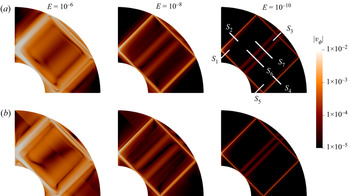
These regions are chosen such that all the rays within them follow the same circuit. Note that we use a logarithmic colour scale over three decades in amplitude. This figure demonstrates that our asymptotic solution can qualitatively reproduce both global and local structures of the internal shear layer at the frequency  $\omega ^*/\varOmega ^*=\sqrt {2}$, especially as the Ekman number becomes small. The wave structure consists of an inclined rectangle and two beams near the centre line
 $z=r$. As the Ekman number decreases, the beams get thinner and their amplitude decreases, which is observed for both asymptotic and numerical solutions. The jumps of the asymptotic solution far away from the critical lines at high Ekman number occur at the endpoints of the calculation regions for every critical line (3.1) which tend to disappear as the Ekman number is reduced and the solution becomes more localised. These jumps may be smoothed by considering the rays outside the regions (3.1) which, however, follow a circuit different from
 $L_1\leftrightarrow L_2\leftrightarrow L_3\leftrightarrow L_4\leftrightarrow L_5$ and are therefore not considered here. In figure 7,
 $S_{1-5}$ are the five sections crossing the main circuit, while
 $S_6$ and
 $S_7$ are crossing the two secondary beams near the centre line
 $z=r$. Quantitative comparisons will be made on these sections in the following.
Contours of amplitudes of azimuthal velocity of numerical (a) and asymptotic (b) solutions for three Ekman numbers  $E=10^{-6}$,
 $10^{-8}$ and
 $10^{-10}$.

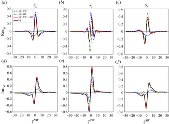
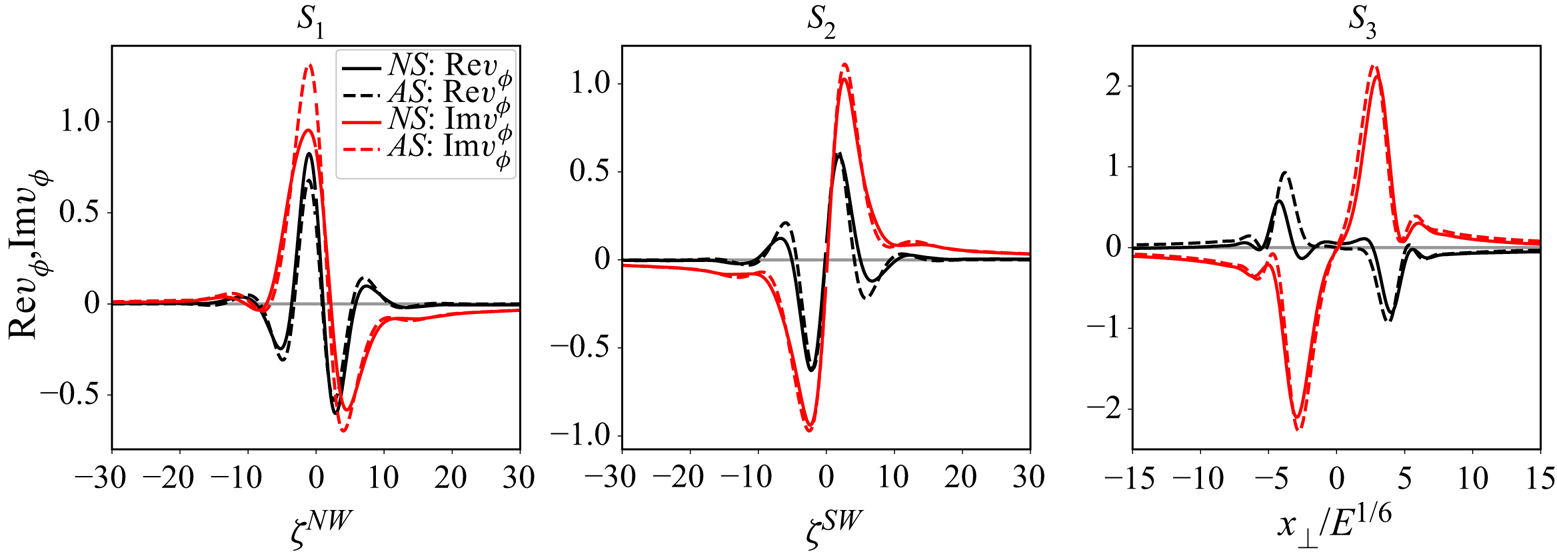
Figure 8 compares the asymptotic velocity profiles for the northward and southward rays independently and their sum with the numerical profiles on three sections ( $S_2$,
 $S_3$ and
 $S_4$) and at an Ekman number of
 $E=10^{-10}$. The northward ray propagates from
 $S_2$ to
 $S_4$, while the southward one propagates from
 $S_4$ to
 $S_2$. Therefore, the amplitude of the northward ray decays from
 $S_2$ to
 $S_4$, while that of the southward ray decays from
 $S_4$ to
 $S_2$. The figure shows that only the superposition of both rays can approximate the numerical solution.
Azimuthal velocity profiles  $v_\phi$ of the asymptotic solution (
 $AS$) for northward and southward rays and the sum of them and the numerical solution (
 $NS$) on three sections (
 $S_2$,
 $S_3$ and
 $S_4$, see figure 7) and at the Ekman number
 $E=10^{-10}$.

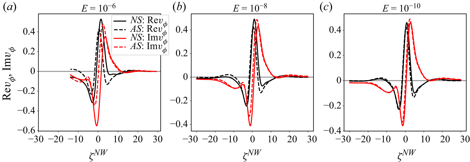
The asymptotic and numerical solutions at different Ekman numbers for the main beams on the section  $S_2$ are compared in figure 9, which shows that our asymptotic solution performs better as the Ekman number decreases, as expected. At the lowest value of
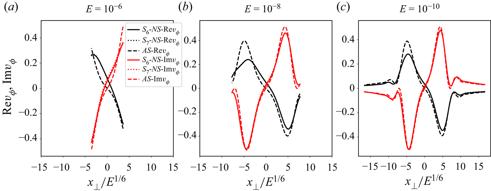
 $E=10^{-10}$, which starts to be relevant for geophysical applications, the agreement between the two solutions is remarkable, even far from the characteristic path. In figure 10, the same comparison is also made for the secondary beams on the sections
 $S_6$ and
 $S_7$. The numerical solutions on two different sections
 $S_6$ and
 $S_7$ are almost the same, which demonstrates the quasi-inviscid propagation of the beams along the critical lines
 $L_6$ and
 $L_8$. Better performance of asymptotic solutions with decreased Ekman number is also observed. Note that in figure 9 the narrower regions of the similarity variables at higher Ekman numbers are caused by the fixed length of the sections. The similarity variables on the sections take wider ranges of values for lower Ekman numbers (see (2.6)). The same is also true for the
 $x_\perp$ scaled with
 $E^{1/6}$ in figure 10.
Azimuthal velocity profiles  $v_\phi$ of the asymptotic and numerical solutions (
 $AS$ and
 $NS$) at three Ekman numbers (
 $E=10^{-6}$,
 $10^{-8}$ and
 $10^{-10}$) for the main beams on the section
 $S_2$.

Same caption as above for the secondary beams on the sections  $S_6$ and
 $S_7$.

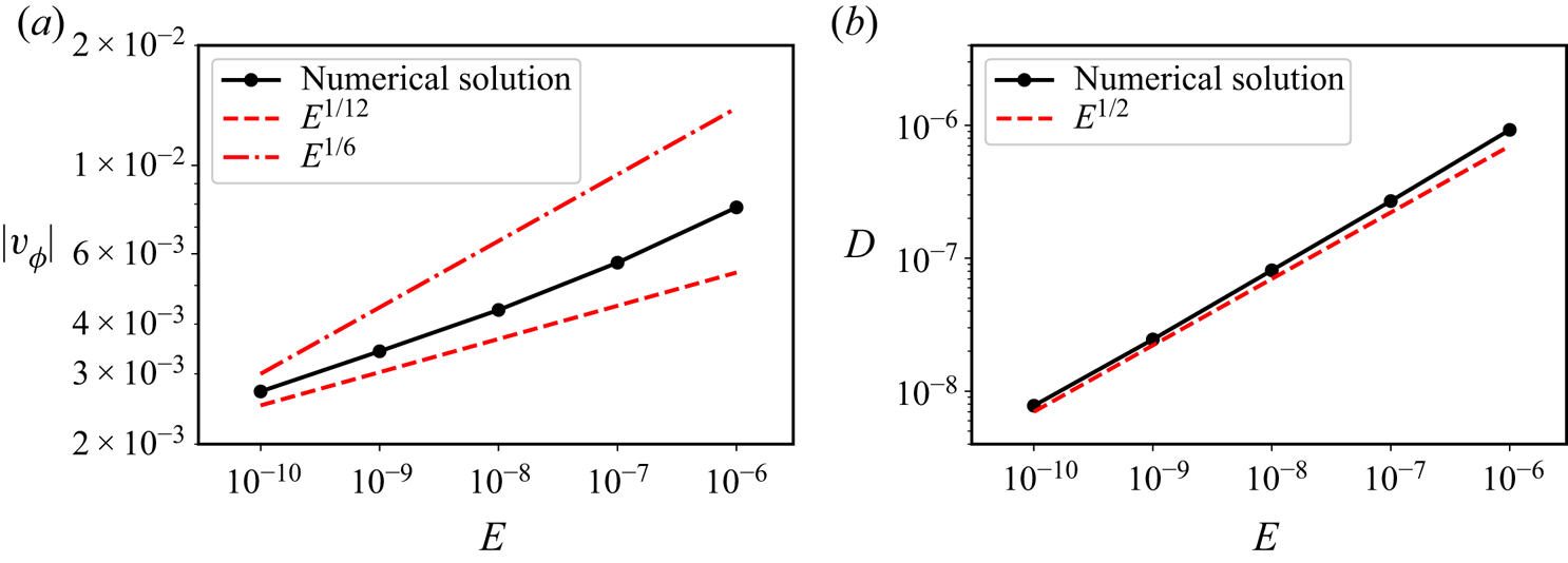
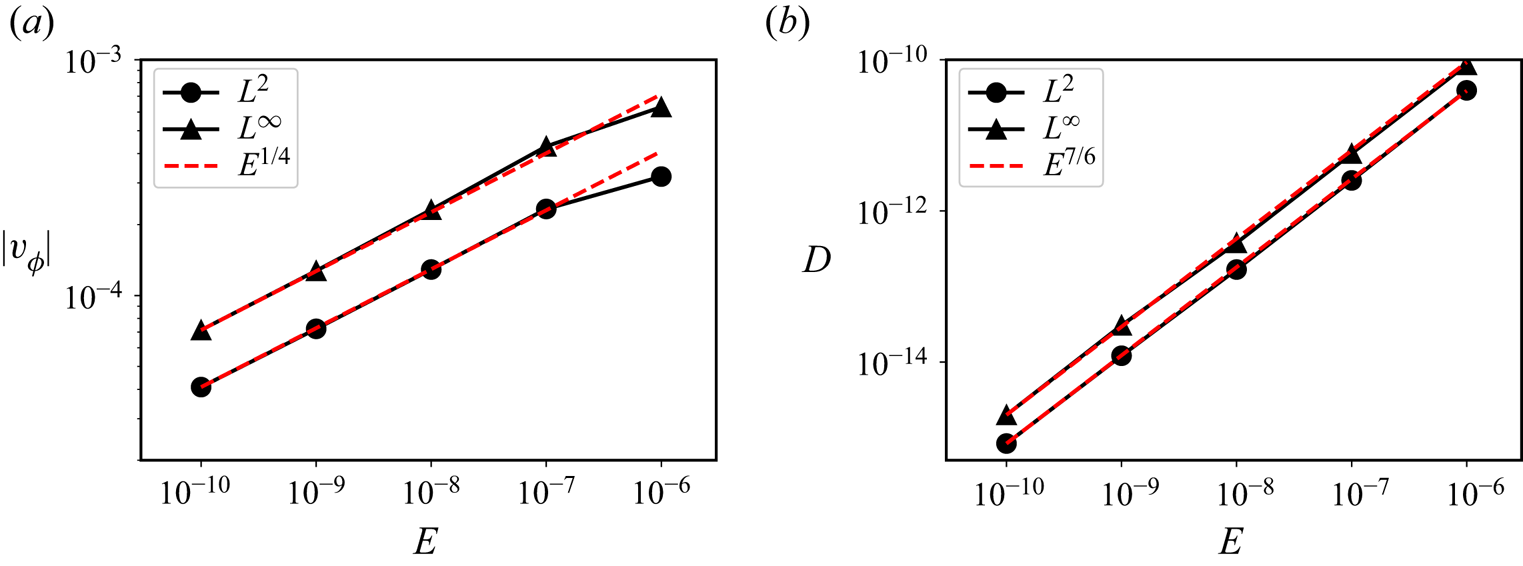
The physical scalings of the numerical results in the range of Ekman number  $10^{-10}\leq E \leq 10^{-6}$ are presented in figures 11 and 12 for the main and secondary beams, respectively. A fixed point at the intersection between the critical line
 $L_2$ and the section
 $S_2$ is selected to measure both velocity amplitude and dissipation rate at various Ekman numbers for the main beams. For the secondary beams, the same quantities are measured on the sections
 $S_6$ and
 $S_7$ in the narrow range
 $-5\leqslant x_\perp /E^{1/6}\leqslant 5$ around the critical lines
 $L_6$ and
 $L_8$ since the quantities are close to zero on the critical lines. Both
 $L^2$ and
 $L^\infty$ norms are considered for Ekman numbers ranging from
 $10^{-6}$ to
 $10^{-10}$, as shown in figure 12. For the
 $L^2$ norm, results are scaled by the square root of the number of points into the region
 $-5\leqslant x_\perp /E^{1/6}\leqslant 5$ since the number of points changes with the Ekman number. Figure 11(a) shows that the velocity amplitude of the main internal shear layer follows the scaling
 $E^{1/12}$ predicted by Le Dizès & Le Bars (Reference Le Dizès and Le Bars2017) for an open geometry. This observation is to be contrasted with the scaling
 $E^{1/6}$ assumed by Kerswell (Reference Kerswell1995), who actually extrapolated the scaling of the shear layer emitted by an oscillating split disc to the one emitted by a librating inner core. The foregoing numerical results show that this simple extrapolation is not valid. We note that our results also further confirm the numerical observation made by Lin & Noir (Reference Lin and Noir2021) at comparatively higher Ekman numbers, where the scaling
 $E^{1/12}$ was favoured over
 $E^{1/6}$. For the secondary beams, figure 12(a) shows that the amplitude of the velocity also follows the predicted scaling
 $E^{1/4}$. Regarding the dissipation rate, it follows the expected
 $E^{1/2}$ and
 $E^{7/6}$ scalings for the main and secondary beams, respectively. These scalings imply that the power dissipated by the respective beams vanishes as
 $E^{5/6}$ and
 $E^{4/3}$, which is weaker than the
 $E^{1/2}$ dissipation within the Ekman boundary layers. Libration in the whole shell is therefore mainly dissipated in the Ekman boundary layers.


Same caption as in figure 11 but with quantities measured in the sections  $S_6$ and
 $S_7$ around
 $L_6/L_8$ in the range
 $-5\leqslant x_\perp /E^{1/6}\leqslant 5$.

Excluding the dissipation in the boundary layers by using stress-free boundary conditions, Rieutord & Valdettaro (Reference Rieutord and Valdettaro2010) also found a vanishing dissipation as  $E\rightarrow 0$ but with a lower power, namely as
 $E^{2/5}$ (see their figure 12). However, Rieutord & Valdettaro (Reference Rieutord and Valdettaro2010) forced the oscillating flow with an
 ${{O}}(1)$ body force, while in the present case the forcing vanishes as
 $E\rightarrow 0$. This latter point underlines the importance of the nature of the forcing in the response of the fluid and the associated viscous dissipation.
The errors of the asymptotic solution relative to the numerical one are measured on the five sections  $S_{1-5}$ in the narrow range
 $-10\leqslant \zeta \leqslant 10$ around the critical lines
 $L_1\text{--}L_5$ for the main beams. They are also computed on the two sections
 $S_{6-7}$ in the narrow range
 $-5\leqslant x_\perp /E^{1/6}\leqslant 5$ around the critical lines
 $L_6$ and
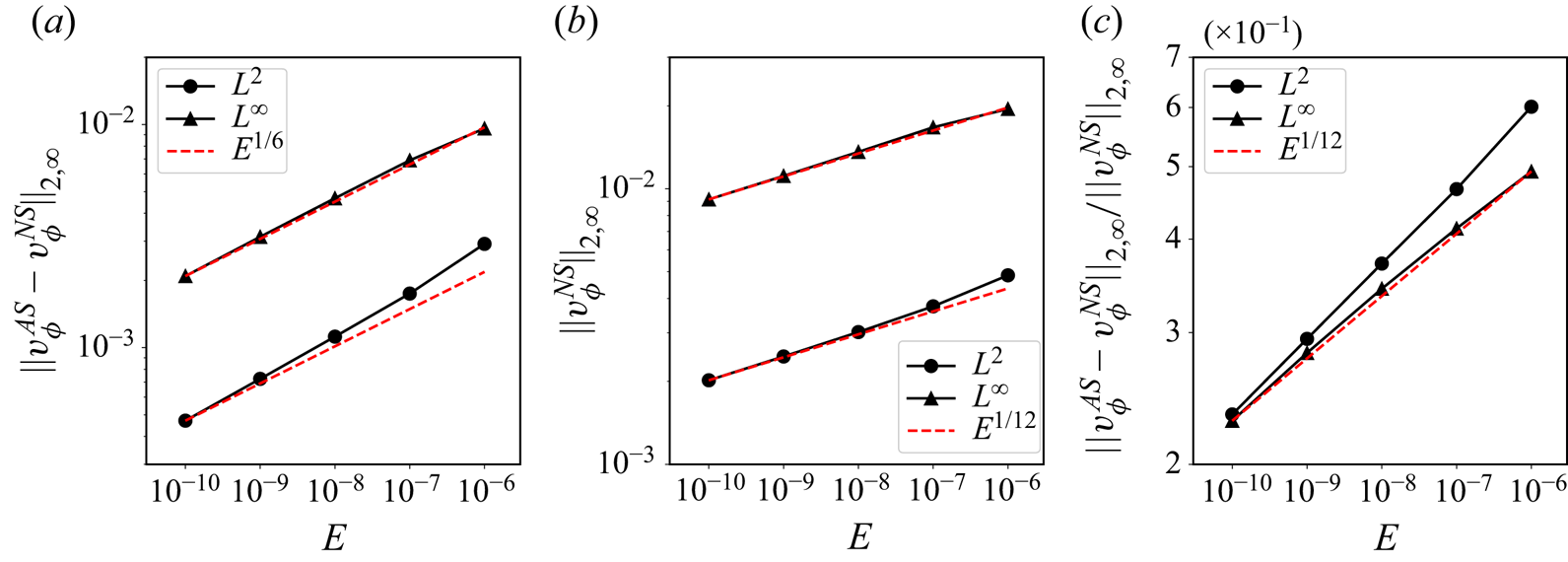
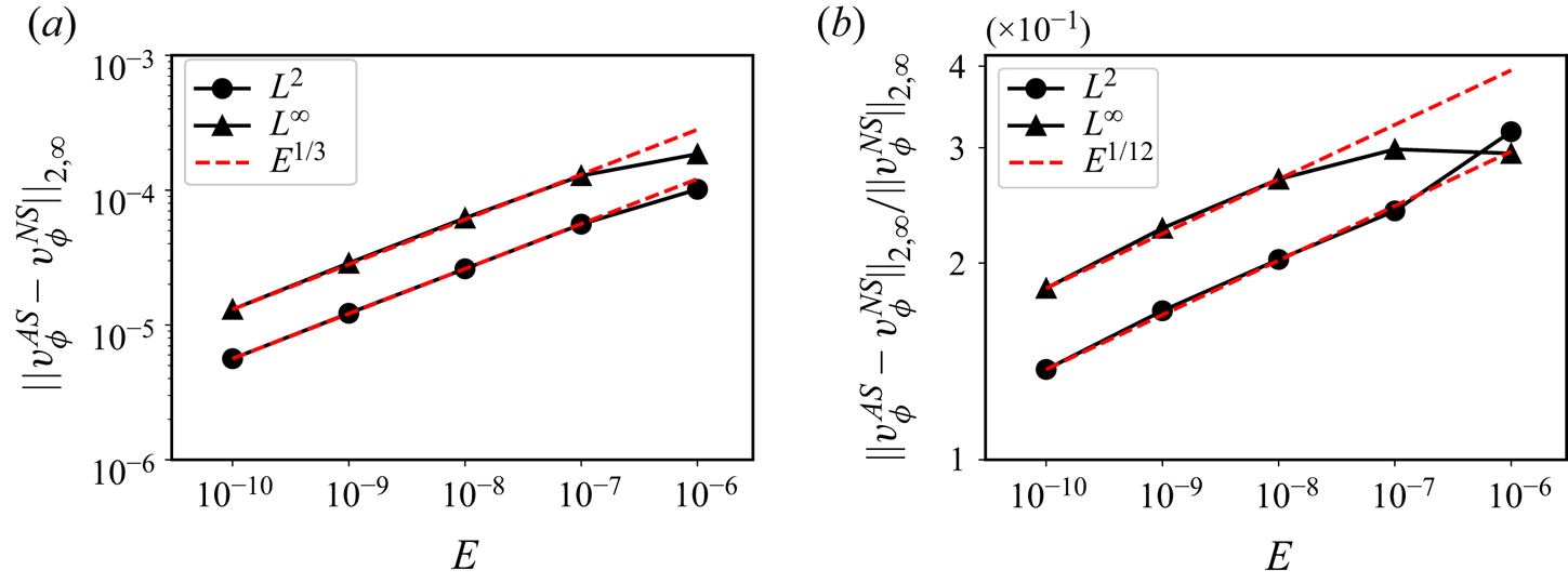
 $L_8$ for the secondary beams (see figures 3 and 7). The solution in these narrow regions is negligibly affected by the boundaries, the axis and the critical latitude where the asymptotic solution is not expected to perform well. The absolute error is measured by the norm of the difference between the theoretical predictions and numerical results averaged over the region of interest around the beam. The relative error between the two approaches is obtained by normalising with the reference numerical solution. The absolute error plotted in figure 13(a) for the main beams is shown to scale with
 $E^{1/6}$ for both
 $L^2$ and
 $L^\infty$ norms, while that for the secondary beams shown in figure 14(a) scales with
 $E^{1/3}$. Figure 13(b) demonstrates that the scaling in
 $E^{1/12}$ of the numerical solution for the main beams is very well predicted if we focus on the beam near the critical lines, similar to that for the secondary beams shown in figure 12(a). The relative errors for the main and secondary beams given in figures 13(c) and 14(b) follow the same scaling in
 $E^{1/12}$ as expected.
Absolute and relative errors on the azimuthal component of the velocity between the asymptotic and numerical solutions as a function of the Ekman number. The quantities are computed in the five sections  $S_{1-5}$ defined in figure 7 in the range of
 $-10\leqslant \zeta \leqslant 10$.


3.2. Aspect ratio $\eta =1/\sqrt {2}$

We now consider the comparison between the theoretical asymptotic predictions and numerical results in a spherical shell with an aspect ratio of  $\eta =1/\sqrt {2}$. The reason behind this choice is the peculiar nature of the critical path, which connects the critical latitude to the pole and the equator without reflection on the boundaries. We use the same asymptotic approach as described previously.
Figure 15 compares the contours of the amplitude of the azimuthal velocity at  $E=10^{-10}$. Once again, our asymptotic solution can reproduce the beam structure, including the secondary weaker beam which corresponds to secondary reflections on the inner core close to the critical latitude. The velocity profiles are compared in figure 16 for the three sections defined in figure 15. We can see that a good agreement is obtained, even for this more pathological case involving reflections near the poles. The convergence properties as the Ekman number is reduced are the same as for the previous case
 $\eta =0.35$.
Contours of  $|v_\phi |$ at
 $E=10^{-10}$ and
 $\eta =1/\sqrt {2}$ by numerical (a) and asymptotic (b) methods.

Velocity profiles along the three sections shown in figure 15 for  $E=10^{-10}$ and
 $\eta =1/\sqrt {2}$.

4. Solution close to the axis
The self-similar solution (2.28) is singular on the axis due to the term  $1/\sqrt {r}$. The region close to the axis has therefore been ignored in the asymptotic results discussed so far. Around the axis, the velocity and pressure can be expressed using Hankel transforms, as done by Le Dizès & Le Bars (Reference Le Dizès and Le Bars2017) in an open geometry. In this section, we generalise this approach to the case of the spherical shell where the asymptotic solution now involves a series of rays propagating in opposite directions.
4.1. Asymptotic theory
We consider the reflections on the axis at the intersection of two adjacent critical lines  $L_1$ and
 $L_2$ shown in figure 3 for the aspect ratio
 $\eta =0.35$. In the spherical shell, two types of rays are involved there: the northward rays that reflect from
 $L_1$ to
 $L_2$, and the southward ones that reflect from
 $L_2$ to
 $L_1$ after having performed two reflections on the outer sphere. Far away from the axis, the self-similar solution (2.28) holds. Close to the axis, the following Hankel transform for the velocity components and pressure can be used:
 $$\begin{gather} v_r= \int_0^\infty U_1(k)J_1(kr)\, {\rm e}^{\mathrm{i}\mu_1z}\, {\rm d} k+\int_0^\infty U_2(k)J_1(kr)\, {\rm e}^{\mathrm{i}\mu_2z}\, {\rm d} k, \end{gather}$$
 $$\begin{gather}v_\phi= \int_0^\infty V_1(k)J_1(kr)\, {\rm e}^{\mathrm{i}\mu_1z}\, {\rm d} k+\int_0^\infty V_2(k)J_1(kr)\, {\rm e}^{\mathrm{i}\mu_2z}\, {\rm d} k, \end{gather}$$
 $$\begin{gather}v_z= \int_0^\infty W_1(k)J_0(kr)\, {\rm e}^{\mathrm{i}\mu_1z}\, {\rm d} k+\int_0^\infty W_2(k)J_0(kr)\, {\rm e}^{\mathrm{i}\mu_2z}\, {\rm d} k, \end{gather}$$
 $$\begin{gather}p= \int_0^\infty P_1(k)J_0(kr)\, {\rm e}^{\mathrm{i}\mu_1z}\, {\rm d} k+\int_0^\infty P_2(k)J_0(kr)\, {\rm e}^{\mathrm{i}\mu_2z}\, {\rm d} k, \end{gather}$$
where  $J_\alpha$(
 $\alpha =0,1$) are the Bessel functions of the first kind and
 $\mu _1$ and
 $\mu _2$ are inviscid wavenumbers corresponding to the northward and southward rays, respectively. The four other viscous wavenumbers that could also be present in (4.1) (see Le Dizès Reference Le Dizès2015) have been omitted here because they are not present in the internal shear layer structure and not needed to smooth the singularity on the axis, as we shall see. Note also that, in an open geometry, only the component
 $\mu _1$ associated with the northward ray is used (Le Dizès & Le Bars Reference Le Dizès and Le Bars2017), since the southward ray goes to infinity and never comes back close to the axis. At leading order, the two inviscid wavenumbers are related to
 $k$ by
 \begin{equation} \mu_1=k\frac{\cos\theta_c}{\sin\theta_c}, \quad \mu_2={-}k\frac{\cos\theta_c}{\sin\theta_c}. \end{equation}
The corresponding amplitudes  $(U_1,V_1,W_1,P_1)$ and
 $(U_2,V_2,W_2,P_2)$ are related to each other by the following expressions (Le Dizès Reference Le Dizès2015):
 $$\begin{gather} U_{1,2}= \mathrm{i}\cos\theta_cV_{1,2}, \end{gather}$$
 $$\begin{gather}W_1={-}\sin\theta_cV_1, \end{gather}$$
 $$\begin{gather}W_2= \sin\theta_cV_2, \end{gather}$$
 $$\begin{gather}kP_{1,2}={-}2\sin\theta_cV_{1,2}. \end{gather}$$
To describe the solution close to the reflection point on the axis, of coordinates  $(0,\eta /\cos \theta _c)$, we introduce the local variables
 \begin{equation} \tilde{r}=r/E^{1/3}, \quad \tilde{z}=(z-\eta/\cos\theta_c)/E^{1/3}. \end{equation}
The Hankel transform (4.1) can then be written as
 $$\begin{gather} v_r= \mathrm{i}\cos\theta_c \left[\int_0^\infty \tilde{V}_1J_1(\tilde{k}\tilde{r})\, {\rm e}^{\mathrm{i}\tilde{k}\gamma\tilde{z}}\, {\rm d} \tilde{k}+\int_0^\infty \tilde{V}_2J_1(\tilde{k}\tilde{r})\, {\rm e}^{-\mathrm{i}\tilde{k}\gamma\tilde{z}}\, {\rm d} \tilde{k}\right], \end{gather}$$
 $$\begin{gather}v_\phi= \int_0^\infty \tilde{V}_1J_1(\tilde{k}\tilde{r})\, {\rm e}^{\mathrm{i}\tilde{k}\gamma\tilde{z}}\, {\rm d} \tilde{k}+\int_0^\infty \tilde{V}_2J_1(\tilde{k}\tilde{r})\, {\rm e}^{-\mathrm{i}\tilde{k}\gamma\tilde{z}}\, {\rm d} \tilde{k}, \end{gather}$$
 $$\begin{gather}v_z= \sin\theta_c\left[-\int_0^\infty \tilde{V}_1J_0(\tilde{k}\tilde{r})\, {\rm e}^{\mathrm{i}\tilde{k}\gamma\tilde{z}}\, {\rm d} \tilde{k}+\int_0^\infty \tilde{V}_2J_0(\tilde{k}\tilde{r})\, {\rm e}^{-\mathrm{i}\tilde{k}\gamma\tilde{z}}\, {\rm d} \tilde{k}\right], \end{gather}$$
 $$\begin{gather}p={-}2\sin\theta_cE^{{1}/{3}}\left[\int_0^\infty \tilde{V}_1\frac{J_0(\tilde{k}\tilde{r})}{\tilde{k}}\, {\rm e}^{\mathrm{i}\tilde{k}\gamma\tilde{z}}\, {\rm d} \tilde{k}+\int_0^\infty \tilde{V}_2\frac{J_0(\tilde{k}\tilde{r})}{\tilde{k}}\, {\rm e}^{-\mathrm{i}\tilde{k}\gamma\tilde{z}}\, {\rm d} \tilde{k}\right], \end{gather}$$
with  $\gamma =1/\tan \theta _c$.
Expressions for  $\tilde {V}_1$ and
 $\tilde {V}_2$ are sought by matching the solution close to the axis (4.5) with the self-similar solution in the bulk ((2.28) and (2.10)). When both
 $\tilde {r}$ and
 $\tilde {z}$ go to infinity, the limit of
 $v_\phi$ (4.5b) is
 \begin{align} v_\phi&\sim\frac{1}{\sqrt{2{\rm \pi}\tilde{r}}}\int_0^{\infty} \frac{\tilde{V}_1(\tilde{k})}{\sqrt{\tilde{k}}}\, {\rm e}^{\mathrm{i} \tilde{k}(\tilde{r}+\gamma\tilde{z})-\mathrm{i}3{\rm \pi}/4}\, {\rm d} \tilde{k} \end{align}
 \begin{align} &\quad +\frac{1}{\sqrt{2{\rm \pi}\tilde{r}}}\int_0^{\infty}\frac{\tilde{V}_1(\tilde{k})}{\sqrt{\tilde{k}}}\, {\rm e}^{\mathrm{i}\tilde{k}(-\tilde{r}+\gamma\tilde{z})+\mathrm{i}3{\rm \pi}/4}\, {\rm d} \tilde{k} \end{align}
 \begin{align} &\quad +\frac{1}{\sqrt{2{\rm \pi}\tilde{r}}}\int_0^{\infty}\frac{\tilde{V}_2(\tilde{k})}{\sqrt{\tilde{k}}}\, {\rm e}^{\mathrm{i}\tilde{k}(\tilde{r}-\gamma\tilde{z})-\mathrm{i}3{\rm \pi}/4}\, {\rm d} \tilde{k} \end{align}
 \begin{align} &\quad +\frac{1}{\sqrt{2{\rm \pi}\tilde{r}}}\int_0^{\infty}\frac{\tilde{V}_2(\tilde{k})}{\sqrt{\tilde{k}}}\, {\rm e}^{\mathrm{i}\tilde{k}(-\tilde{r}-\gamma\tilde{z})+\mathrm{i}3{\rm \pi}/4}\, {\rm d} \tilde{k}, \end{align}
using the asymptotic behaviour of the Bessel function at infinity. The four components correspond to the incident northward rays ( $L_1$), the reflected northward rays (
 $L_2$), the incident southward rays (
 $L_2$) and the reflected southward rays (
 $L_1$). The former two components for the incident and reflected northward rays imply that there is a phase shift from the incident to reflected rays, which is
 $3{\rm \pi} /2$ for the azimuthal velocity. Considering the phase (2.10) between
 $v_\parallel$ and
 $v_\phi$, the phase shift for
 $v_\parallel$ is
 ${\rm \pi} /2$. The same is true for the southward rays.
On the other hand, the self-similar solution ((2.28) and (2.10)) for  $v_\phi$ in the bulk takes the following form close to the intersection point on the axis (
 $r\rightarrow 0, z\rightarrow \eta /\cos \theta _c$):
 \begin{align} v_\phi&\sim\mathrm{i}\frac{1}{\sqrt{r}}C_0^{NW}G_m (L_{NW},\sin\theta_c(\tilde{r}+\gamma\tilde{z}),L) \end{align}
 \begin{align} &\quad +\frac{1}{\sqrt{r}}C_0^{NW}G_m (L_{NW},\sin\theta_c(-\tilde{r}+\gamma\tilde{z}),L) \end{align}
 \begin{align} &\quad +\mathrm{i}\frac{1}{\sqrt{r}}C_0^{SW}G_m (L_{SW},\sin\theta_c(\tilde{r}-\gamma\tilde{z}),L) \end{align}
 \begin{align} &\quad +\frac{1}{\sqrt{r}}C_0^{SW}G_m (L_{SW},\sin\theta_c(-\tilde{r}-\gamma\tilde{z}),L), \end{align}
where  $L_{NW}$ and
 $L_{SW}$ are the travelled distances of the northward and southward rays from the source to the intersection point on the axis, respectively. Here,
 $L$ is the travelled distance within one cycle (2.20).
By matching (4.6) with (4.7), the amplitudes  $\tilde {V}_1$ and
 $\tilde {V}_2$ are obtained as follows:
 $$\begin{gather} \tilde{V}_1= E^{{-}1/6}C_0^{NW}\sqrt{2{\rm \pi}} \frac{\tilde{k}^{m-1/2}}{\sin^m\theta_c}\, {\rm e}^{\mathrm{i}5{\rm \pi}/4} \frac{{\rm e}^{-\mathrm{i}m{\rm \pi}/2}}{(m-1)!}\frac{{\rm e}^{{-}L_{NW} \tilde{k}^3/(2\sin^4\theta_c)}}{1-\mathrm{i}\, {\rm e}^{{-}L \tilde{k}^3/(2\sin^4\theta_c)}}, \end{gather}$$
 $$\begin{gather}\tilde{V}_2= E^{{-}1/6}C_0^{SW}\sqrt{2{\rm \pi}}\frac{\tilde{k}^{m-1/2}}{\sin^m\theta_c} \, {\rm e}^{\mathrm{i}5{\rm \pi}/4}\frac{{\rm e}^{-\mathrm{i}m{\rm \pi}/2}}{(m-1)!} \frac{{\rm e}^{{-}L_{SW}\tilde{k}^3/(2\sin^4\theta_c)}}{1- \mathrm{i}\, {\rm e}^{{-}L\tilde{k}^3/(2\sin^4\theta_c)}}. \end{gather}$$
It is worth pointing out the factor  $E^{-1/6}$ in front of the ray amplitudes
 $C_0^{NW}$ and
 $C_0^{SW}$. These amplitudes are
 ${{O}}(E^{1/12})$, which means that
 $\tilde {V}_1$ and
 $\tilde {V}_2$ scale as
 $E^{-1/12}$. This implies that the solution close to the reflection point is expected to grow infinitely as
 $E$ goes to zero. It clearly shows the singular nature of the small Ekman number limit for this problem: the linear solution is expected to vanish everywhere except in the boundary layer on the inner sphere (where it is finite) and at this single reflection point on the axis (where it diverges).
4.2. Comparison with numerical results
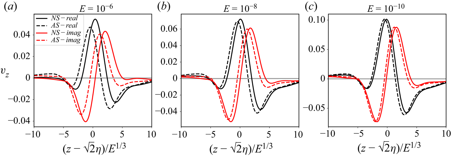
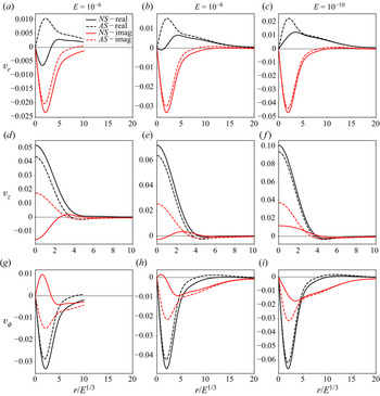
The asymptotic solution close to the axis (4.5) with the amplitudes (4.8) is compared with the numerical results. Figure 17 compares the asymptotic and numerical solutions along the rotation axis for three Ekman numbers. Only the velocity component  $v_z$ is concerned, as the other two components are zero by axisymmetry. We obtain a good agreement between the theoretical predictions and the numerical results. As the Ekman number decreases, our asymptotic solution converges to the numerical one. Figure 18 shows the same comparison but on the line perpendicular to the rotation axis and passing by the reflection point
 $(0,\eta /\cos \theta _c)$. All three velocity components are considered. Contrary to previous results, only one part of the asymptotic solution (namely the imaginary part of
 $v_r$ and the real part of
 $v_z$ and
 $v_\phi$) performs well. However, as we decrease the Ekman number, the other part of the asymptotic solution approaches the corresponding numerical one, although there are still obvious differences for our lowest Ekman number
 $10^{-10}$. Interestingly, the absolute errors of the asymptotic solution close to axis are found to be almost invariant with the Ekman number (not shown here), while the relative errors scale with
 $E^{1/12}$ similarly to those in the bulk (see figures 13c and 14b). This suggests that both the errors of the asymptotic solutions close to axis and in the bulk come from the same source, which could be a weaker singularity at the critical latitude. It is suspected that the order of this singularity is
 ${{O}}(E^{1/6})$, which corresponds to
 $m=1$ if its solution is still self-similar. Its contribution to the asymptotic solution is not considered here, since we are concerned with the leading-order response, but could be further investigated in future studies.
Comparison of asymptotic solutions and numerical results of  $v_z$ on the axis for three Ekman numbers.

Comparison of asymptotic solutions and numerical results of three velocity components on the line perpendicular to the axis at the reflection point  $(0,\eta /\cos \theta _c)$ for three Ekman numbers.

5. Conclusion
Using both numerical and asymptotic methods, we have studied the harmonic response that is generated in a rotating spherical shell by librating the inner sphere at the frequency  $\omega = \sqrt {2} \varOmega$ where
 $\varOmega$ is the angular frequency of the fluid. For this particular frequency, the inertial waves propagate along rays inclined at
 $45$ degrees with respect to the equatorial plane and therefore form closed periodic orbits in a spherical shell. We have shown, by considering numerical results down to Ekman numbers
 $E=10^{-10}$, that the harmonic response is mainly governed by the internal shear layers that are emitted from the critical latitude of the inner sphere. In Le Dizès & Le Bars (Reference Le Dizès and Le Bars2017), it was shown that these internal shear layers are concentrated wave beams that can be described in an open geometry and at small Ekman numbers by the similarity solution initially introduced by Moore & Saffman (Reference Moore and Saffman1969). Here, we have further generalised this model and constructed an asymptotic solution by monitoring the reflections of the critical-latitude beams on the boundaries and on the axis. Despite the curvature of the boundaries, owing to the large-wavenumber approximation (Baines Reference Baines1971a), the reflection laws on a locally planar boundary (Le Dizès Reference Le Dizès2020) can be applied to construct the self-similar form of the main
 $E^{1/3}$ shear layers. The diffraction (Baines Reference Baines1971b) on the inner boundary creates a secondary
 $E^{1/6}$ shear layer whose asymptotic form is not self-similar. The two asymptotic forms give the scalings of the velocity amplitudes in
 $E^{1/12}$ and
 $E^{1/4}$ for the main and secondary shear layers, respectively. The respective local dissipation rates are predicted to scale with
 $E^{1/2}$ and
 $E^{7/6}$. We have finally obtained that the asymptotic solution can be written as an infinite sum of similarity solutions for the main shear layers. Interestingly, this sum converges owing to the phase shift of
 ${\rm \pi} /2$ that the beams experience at each reflection on the rotation axis. The same summation strategy can also be applied for the non-self-similar form of the secondary shear layers and a convergent sum is thus obtained for the same reason.
The asymptotic solution has been compared with the numerical solution of the linearised equations for several Ekman numbers and two values of the shell aspect ratio, and a very good agreement has been demonstrated. The relative error has been shown to be of order  $E^{1/12}$. We suspect that it could be associated with a weaker singularity at the critical latitude. An immediate consequence of our result is the scaling in
 $E^{1/12}$ of the harmonic response velocity, as predicted for the internal shear layer amplitude in an open geometry (Le Dizès & Le Bars Reference Le Dizès and Le Bars2017). This scaling was also observed in recent simulations by Lin & Noir (Reference Lin and Noir2021) but it contrasts with the
 $E^{1/6}$ scaling previously reported in the literature in similar contexts (Kerswell Reference Kerswell1995; Calkins et al. Reference Calkins, Noir, Eldredge and Aurnou2010; Favier et al. Reference Favier, Barker, Baruteau and Ogilvie2014; Cébron et al. Reference Cébron, Laguerre, Noir and Schaeffer2019).
We have also analysed the solution close to the point on the rotation axis where the critical-latitude beam reflects. The similarity solution diverges at this point. We have provided a new asymptotic expression describing the solution in the  ${{O}}(E^{1/3})$ neighbourhood of this point. We have in particular shown that the solution also scales as
 $E^{-1/12}$ in this region.
It is worth emphasising that the theoretical method that has been used to build the asymptotic solution can be applied to other situations. For instance, one can imagine considering other libration frequencies. As long as  $\omega < 2 \varOmega$, critical-latitude beams are expected to be excited. These beams would propagate in the spherical shell, be reflected on boundaries and form a complex ray pattern depending on the aspect ratio and the frequency. If the critical-latitude beams converge towards an attractor, or if they travel along a periodic orbit, as in the present case, the solution is expected to be localised along these beams. The solution could then be obtained as a sum of similarity solutions. Because these similarity solutions decrease slowly along their direction of propagation as
 $x_\parallel ^{-5/12}$, the convergence of this sum would depend on the phase shift that the beam experiences on the periodic orbit or on the attractor, that is on the number of reflections on the axis. If the sum converges, we claim that our approach should apply. The other situation where the sum does not converge is naturally of interest. We suspect that in that case one obtains a completely different response with a new scaling in
 $E$, and probably multi-layer structures as observed in the Stewartson layers between differentially rotating spheres (Stewartson Reference Stewartson1966).
Finally, it is important to mention that we have limited our analysis to libration to be able to use an existing model for the structure of the critical-latitude beam. Yet, critical-latitude beams exist for other types of harmonic forcing. One similar viscous forcing is the precession of a spherical shell for which the critical-latitude beams are inclined at  $30\,^\circ$ with respect to the rotation axis and form a periodic orbit if the inner core radius is smaller than half the outer one (Hollerbach & Kerswell Reference Hollerbach and Kerswell1995). The asymptotic solution obtained in the present paper for libration is expected to work similarly in that case with the same singularity strength (
 $m=5/4$) for the critical latitude beam. The modification associated with the azimuthal dependence of precession is indeed expected to just add a phase factor to the solution.
Another stronger forcing is the periodic translation of a sphere generating the famous Saint Andrews cross pattern (Mowbray & Rarity Reference Mowbray and Rarity1967; Greenspan Reference Greenspan1968) which is nothing but the pattern left by the critical-latitude beams. If these beams can be described by the similarity solution of Moore & Saffman (Reference Moore and Saffman1969), a similar approach could then naturally be developed in those cases and further generalised to closed geometries.
Acknowledgements
Centre de Calcul Intensif d'Aix-Marseille is acknowledged for granting access to its high performance computing resources. The authors are grateful to an anonymous reviewer for a decisive comment concerning curvature effects and the weaker central beam which drastically improved the paper.
Funding
J.H. acknowledges China Scholarship Council for financial support (CSC 202008440260).
Declaration of interests
The authors report no conflict of interest.
Appendix A. Justification of the absence of back-reflected beams
In this section, our objective is to show that no back-reflected beams are present when the beam described by the similarity solution reflects on a curved boundary. This result is obtained by proving that this beam is composed of wavelengths which are small compared with the radius of curvature of the boundary. For this purpose, one just has to notice that the similarity solution ((2.5)–(2.7)) is given by an integral of the form
 \begin{equation} I = \int_0^\infty \, {\rm e}^{\mathrm{i}p({x_\perp}/{E^{1/3}})}\, {\rm e}^{{-}p^3({x_\parallel}/{2\sin\theta_c})}p^{m-1}\, {\rm d} p, \end{equation}
and that, since this integral converges for any  $m>0$ and
 $x_\parallel >0$, we can replace the boundaries 0 and
 $\infty$ of the integral by
 $\varepsilon$ and
 $1/\varepsilon$ for any
 $\varepsilon \rightarrow 0$. Thus, after a change of integration variable we obtain
 \begin{equation} I\sim E^{m/3}\int_{\varepsilon/E^{1/3}}^{(1/\varepsilon)/E^{1/3}}\, {\rm e}^{\mathrm{i}\tilde{p}x_\perp}\, {\rm e}^{{-}E\tilde{p}^3({x_\parallel}/{2\sin\theta_c})}\tilde{p}^{m-1}\, {\rm d} \tilde{p}. \end{equation}
The first term  $\textrm {e}^{\mathrm {i}\tilde {p}x_\perp }$ of the integrand denotes the carrier with
 $\tilde {p}$ as the wavenumber, while the rest can be considered as the amplitude. If we choose
 $\varepsilon =E^{1/6}$, the wavenumbers fall into the following interval:
 \begin{equation} E^{{-}1/6}<\tilde{p}< E^{{-}1/2}, \end{equation}
which means that the wavenumbers are large in the small Ekman number limit. In other words, the wavelengths governing the similarity solution are small compared with the  $O(1)$ scale of the boundary. As explained in Baines (Reference Baines1971a), this guarantees that the reflection of the beam on the boundary is as if the boundary was locally flat. No back-reflected beams are therefore created.