1 Introduction
The logarithmic dependence of mean velocity profile is the most fundamental feature in wall-bounded turbulent shear flow. The original derivation of von Kármán (Reference von Kármán1930) is based on the mixing length hypothesis (Prandtl Reference Prandtl1925) for modelling of Reynolds shear stress in a pressure-driven plane channel flow. Since the mixing length in the region close to the wall (
 $y/h<0.2$
, where
 $y$
is the wall-normal direction and
 $h$
is the half-height of the channel) has to vanish at the wall, the only possible length scale in this region becomes the distance from the wall (i.e.
 $y$
). Given that the mixing length is conceptually identical to the mean free path in thermodynamics, this indicates that the correlation length scale of fluid motions (i.e. integral length scale) in the logarithmic region would be the distance from the wall. Townsend (Reference Townsend1956, Reference Townsend1976) hypothesised that it would be difficult to imagine the emergence of this feature, unless the size of energy-containing eddies (coherent structures) in the logarithmic region is proportional to the distance from their centre to the wall, and, in this sense, these energy-containing eddies should be ‘attached’ to the wall (i.e. the attached eddy hypothesis). He further assumed that these energy-containing eddies are self-similar and that their near-wall behaviour could be modelled in the inviscid limit. By linearly superposing a generic form of second-order statistical moment of each of the self-similar energy-containing eddies subject to the constant Reynolds shear stress, he predicted that the turbulence intensity of wall-parallel velocity components would be a logarithmically dependent function in the wall-normal direction. For the past two decades, there has been growing evidence that supports the attached eddy hypothesis, and, in particular, recent measurements have confirmed that the theoretical prediction of Townsend (Reference Townsend1976) is indeed a reliable first approximation of turbulence intensities in the logarithmic region (e.g. Marusic et al.
Reference Marusic, Monty, Hultmark and Smits2013). For further details, the reader may refer to the recent review by Marusic & Monty (Reference Marusic and Monty2019) and the references therein.
In the original theory of Townsend (Reference Townsend1976), the detailed form and dynamical feature of individual attached eddies are not required to construct the logarithmic wall-normal dependence of turbulence intensity of wall-parallel velocity components, because the attached eddies are characterised only by the second-order ‘statistical moments’. Indeed, in earlier studies, the form of the attached eddies was modelled only in a statistical manner by taking the flow field observations available at the time. For example, Townsend (Reference Townsend1976) himself proposed a double-cone vortex as a statistical model of individual attached eddies from the experimental observation by Kline et al. (Reference Kline, Reynolds, Schraub and Runstadler1967) on the near-wall streaks. In the refining work by Perry & Chong (Reference Perry and Chong1982), a ‘
 $\unicode[STIX]{x039B}$
’-shaped vortex was adopted from the flow visualisation of Head & Bandyopadhay (Reference Head and Bandyopadhay1981) in a turbulent boundary layer. More recently, Woodcock & Marusic (Reference Woodcock and Marusic2015) considered a fairly generic statistical model of attached eddies, given in the form of spanwise alternating streamwise velocity with finite streamwise size.
Nevertheless, the question of what the main energy-containing eddies really are is very important, as these eddies would play the central role in momentum and mass transfer due to their energy-containing nature – indeed, it was recently shown that the energy-containing eddies which scale with the distance from the wall are the dominant source of turbulent skin-friction generation at high Reynolds numbers (de Giovanetti, Hwang & Choi Reference de Giovanetti, Hwang and Choi2016). Recently, some important statistical and dynamical features of these main energy-containing eddies have also been reported. In particular, the energy-containing eddies in the logarithmic region have been repeatedly found to be statistically and dynamically self-similar (Hwang Reference Hwang2015; Hellstöm, Marusic & Smits Reference Hellstöm, Marusic and Smits2016; Hwang & Bengana Reference Hwang and Bengana2016), as hypothesised by Townsend (Reference Townsend1976). These energy-containing eddies have a sustaining mechanism essentially independent of those at other (length and time) scales (Hwang & Cossu Reference Hwang and Cossu2010b , Reference Hwang and Cossu2011). Each of the energy-containing eddies is composed of elongated streaks and vortex packets statistically in the form of quasi-streamwise vortices (Hwang Reference Hwang2015; Hwang & Bengana Reference Hwang and Bengana2016), and its turnover dynamics is remarkably similar to the so-called ‘self-sustaining process’ of near-wall turbulence that involves both linear and nonlinear mechanisms within the given scale (Hamilton, Kim & Waleffe Reference Hamilton, Kim and Waleffe1995; Waleffe Reference Waleffe1997; Schoppa & Hussain Reference Schoppa and Hussain2002). It is important to note that this statistical and dynamical description of the energy-containing eddies integrates all the known coherent structures within the framework of the attached eddy hypothesis (Hwang Reference Hwang2015), including near-wall streaks (Kline et al. Reference Kline, Reynolds, Schraub and Runstadler1967) and quasi-streamwise vortices (Jeong et al. Reference Jeong, Benney, Schoppa and Kim1997) in the near-wall region, self-similar vortex packets and their wakes in the logarithmic region (del Álamo et al. Reference del Álamo, Jiménez, Zandonade and Moser2006), and large-scale (Kovasznay, Kibens & Blackwelder Reference Kovasznay, Kibens and Blackwelder1970) and very-large-scale motions in the outer region (Kim & Adrian Reference Kim and Adrian1999; del Álamo & Jiménez Reference del Álamo and Jiménez2003; Hutchins & Marusic Reference Hutchins and Marusic2007).
The self-sustaining process has been firmly understood as the turbulence generation mechanism, which involves a two-way interaction between streaks and quasi-streamwise vortices (Hamilton et al. Reference Hamilton, Kim and Waleffe1995; Waleffe Reference Waleffe1997): quasi-streamwise vortices significantly amplify streaks via the ‘lift-up’ effect (Butler & Farrell Reference Butler and Farrell1993; del Álamo & Jiménez Reference del Álamo and Jiménez2006; Cossu, Pujals & Depardon Reference Cossu, Pujals and Depardon2009; Pujals et al. Reference Pujals, García-Villalba, Cossu and Depardon2009; Hwang & Cossu Reference Hwang and Cossu2010a ; McKeon & Sharma Reference McKeon and Sharma2010; Willis, Hwang & Cossu Reference Willis, Hwang and Cossu2010), and the amplified streaks subsequently regenerate new quasi-streamwise vortices via streak instability/transient growth and the following nonlinear mechanisms (Hamilton et al. Reference Hamilton, Kim and Waleffe1995; Schoppa & Hussain Reference Schoppa and Hussain2002; Park, Hwang & Cossu Reference Park, Hwang and Cossu2011; Alizard Reference Alizard2015; Cassinelli, de Giovanetti & Hwang Reference Cassinelli, de Giovanetti and Hwang2017; de Giovanetti, Sung & Hwang Reference de Giovanetti, Sung and Hwang2017). Based on this observation, Waleffe (Reference Waleffe1998, Reference Waleffe2001, Reference Waleffe2003) computed a set of non-trivial (relative) equilibrium solutions of the Navier–Stokes equations by cleverly imposing the exact mathematical balance in the two-way interactions between streaks and quasi-streamwise vortices. For the last two decades, a large number of such solutions, in the form of stationary/travelling waves and periodic orbits, have been found (Nagata Reference Nagata1990; Waleffe Reference Waleffe1998; Kawahara & Kida Reference Kawahara and Kida2001; Waleffe Reference Waleffe2003; Faisst & Eckhardt Reference Faisst and Eckhardt2004; Wedin & Kerswell Reference Wedin and Kerswell2004; Hwang, Willis & Cossu Reference Hwang, Willis and Cossu2016, and many others), and their understanding has played a central role in the recent advance in transition and turbulence at low Reynolds number. These solutions are often called ‘exact coherent states’, and they characterise the state-space skeleton of turbulence at low Reynolds numbers (Gibson, Halcrow & Cvitanovic Reference Gibson, Halcrow and Cvitanovic2008; Willis, Cvitanovic & Avila Reference Willis, Cvitanovic and Avila2013, Reference Willis, Cvitanovic and Avila2016; Budanur & Hof Reference Budanur and Hof2017).
Given the close relation between the self-sustaining process and exact coherent states, the existence of the self-sustaining process for individual attached eddies of Townsend (Reference Townsend1976) indicates that such exact coherent states presumably exist at high Reynolds numbers (Hwang Reference Hwang2015; Hwang & Bengana Reference Hwang and Bengana2016). Although computation of such exact coherent states itself does not necessarily indicate that they can be easily reassembled to form invariant solutions for the entire hierarchical organisation of attached eddies with the Navier–Stokes equations, it would at least allow us to gain physical insight into the emergence of such a hierarchy of coherent structures at high Reynolds number. Interestingly, a set of such exact coherent states was very recently reported by Eckhardt & Zammert (Reference Eckhardt and Zammert2018) in plane Couette flow, and it was obtained by properly rescaling and continuing a pair of equilibrium states (EQ7 and EQ8) in Gibson, Halcrow & Cvitanovic (Reference Gibson, Halcrow and Cvitanovic2009) to high Reynolds number. In the present study, we report a new set of such exact coherent states in channel flow, which emerges in the form of relative equilibrium states (travelling waves). The exact coherent states in the present study are obtained using an overdamped simulation, as in Hwang & Bengana (Reference Hwang and Bengana2016), and they are in different form from those found by Eckhardt & Zammert (Reference Eckhardt and Zammert2018) in plane Couette flow (see § 3.3). Near the saddle-node point in their spanwise size
 $L_{z}$
, this new set of exact coherent states is found to asymptotically scale in viscous inner units, indicating that they are associated with the birth of near-wall structures on increasing Reynolds number. Continuation of these solutions to high Reynolds numbers with an eddy viscosity model (Rawat et al.
Reference Rawat, Cossu, Hwang and Rincon2015; Hwang et al.
Reference Hwang, Willis and Cossu2016) further reveals that they underpin the self-sustaining process of self-similar energy-containing eddies in the logarithmic region emerging in the form of Townsend’s attached eddies.
This paper is organised as follows. In § 2, the numerical method for computation of exact coherent states in the present study is presented. Bifurcation, flow structure and statistics of these solutions are then presented in § 3 with continuation to high Reynolds numbers. In that section, the relation of the present solutions to the others is also discussed. Finally, in § 4, scaling of these solutions and the use of eddy viscosity are discussed comprehensively with concluding remarks.
2 Numerical methods
2.1 Simulations
We consider a pressure-driven channel flow, in which the streamwise, wall-normal and spanwise directions are denoted by
 $x$
,
 $y$
and
 $z$
, respectively, and they are interchangeably denoted by
 $x_{1}$
,
 $x_{2}$
and
 $x_{3}$
. The velocity components in these directions are
 $u$
,
 $v$
and
 $w$
, or
 $u_{1}$
,
 $u_{2}$
and
 $u_{3}$
. The computations in the present study are carried out using the Navier–Stokes solver Diablo, which is well documented in Bewley (Reference Bewley2014). In this solver, the streamwise and spanwise directions are discretised using Fourier series with 2/3 dealiasing rule, whereas the wall-normal direction is discretised using second-order central differences. Time integration is performed semi-implicitly by combining the Crank–Nicolson method with a third-order Runge–Kutta method. All the computations in the present study are carried out by imposing a constant volume flow rate across the channel.
Further to direct numerical simulations, a set of overdamped large-eddy simulations is considered by implementing the static Smagorinsky model (Smagorinsky Reference Smagorinsky1963) in the manner of our previous studies (Hwang & Cossu Reference Hwang and Cossu2010b , Reference Hwang and Cossu2011; Hwang Reference Hwang2015; Hwang & Bengana Reference Hwang and Bengana2016), i.e.
 $$\begin{eqnarray}\tilde{\unicode[STIX]{x1D70F}}_{ij}-\frac{\unicode[STIX]{x1D6FF}_{ij}}{3}\tilde{\unicode[STIX]{x1D70F}}_{kk}=-2\unicode[STIX]{x1D708}_{t}\tilde{\unicode[STIX]{x1D61A}}_{ij},\end{eqnarray}$$
with
 $$\begin{eqnarray}\unicode[STIX]{x1D708}_{t}=(C_{s}\tilde{\unicode[STIX]{x1D6E5}})^{2}\tilde{\mathscr{S}}\mathscr{D},\end{eqnarray}$$
where
 $\tilde{\cdot }$
denotes the filtered quantity,
 $\unicode[STIX]{x1D61A}_{ij}$
the strain-rate tensor,
 $C_{s}$
the Smagorinsky constant,
 $\tilde{\unicode[STIX]{x1D6E5}}=(\tilde{\unicode[STIX]{x1D6E5}}_{1}\tilde{\unicode[STIX]{x1D6E5}}_{2}\tilde{\unicode[STIX]{x1D6E5}}_{3})^{1/3}$
the nominal filter width,
 $\tilde{\mathscr{S}}=(2\tilde{\unicode[STIX]{x1D61A}}_{ij}\tilde{\unicode[STIX]{x1D61A}}_{ij})^{1/2}$
the norm of the strain-rate tensor, and
 $\mathscr{D}=1-\exp [-(y^{+}/A^{+})^{3}]$
the van Driest damping function, with
 $A^{+}=25$
(the superscript
 $^{+}$
denotes scaling with viscous inner units, i.e. normalisation by friction velocity
 $u_{\unicode[STIX]{x1D70F}}$
and viscous inner length scale
 $\unicode[STIX]{x1D6FF}_{\unicode[STIX]{x1D708}}(\equiv \unicode[STIX]{x1D708}/u_{\unicode[STIX]{x1D70F}})$
, where
 $\unicode[STIX]{x1D708}$
is the kinematic viscosity). Here, the Smagorinsky constant
 $C_{s}$
is the main control parameter of such an overdamped simulation: its artificial elevation has been used to remove smaller-scale background turbulence, while modelling their role in turbulent transport and dissipation with the artificially elevated eddy viscosity (Hwang & Cossu Reference Hwang and Cossu2010b
). In the present study, this approach is adopted to continue the discovered exact coherent states to higher Reynolds numbers, and the relevance of this approach will be discussed in detail in § 4.2.
In plane channel flow, the spanwise integral length scale of fully developed turbulence typically varies from
 $\unicode[STIX]{x1D706}_{z}^{+}\simeq 100$
to
 $\unicode[STIX]{x1D706}_{z}/h\simeq 1.5$
(Hwang Reference Hwang2015). Therefore, setting the spanwise computational domain
 $L_{z}$
to be a value between the two spanwise integral length scales eliminates any motions with spanwise size greater than
 $L_{z}$
(Hwang Reference Hwang2013). Combining this approach with elevation of
 $C_{s}$
by an appropriate value enables us to isolate self-sustaining motions at
 $\unicode[STIX]{x1D706}_{z}=L_{z}$
, as was shown in Hwang (Reference Hwang2015) and Hwang & Bengana (Reference Hwang and Bengana2016), where these self-sustaining motions were found to be approximately self-similar with respect to the spanwise length scale
 $\unicode[STIX]{x1D706}_{z}$
. Since the goal of the present study is to compute a family of exact coherent states embedded in such self-similar motions, the spanwise domain size
 $L_{z}$
is set as the main control parameter to characterise the size of exact coherent states. The streamwise domain size is subsequently set to be
 $L_{x}=2L_{z}$
, so that the computed exact coherent states fit in the minimal unit for the self-sustaining process of each energy-containing motion in the logarithmic region (Hwang & Cossu Reference Hwang and Cossu2011; Hwang & Bengana Reference Hwang and Bengana2016).
2.2 Exact coherent states
The search for exact coherent states is carried out in the following invariant subspace of the velocity fields:
 $$\begin{eqnarray}\displaystyle [u,v,w,p](x,y,z)=[u,-v,w,p](x,2h-y,z), & & \displaystyle\end{eqnarray}$$
 $$\begin{eqnarray}\displaystyle [u,v,w,p](x,y,z)=[u,v,-w,p](x-L_{x}/2,y,-z). & & \displaystyle\end{eqnarray}$$
 $y=h$
, which is imposed by applying a symmetric boundary condition to the channel centre,
 $\unicode[STIX]{x2202}u/\unicode[STIX]{x2202}y=0,~v=0,~\unicode[STIX]{x2202}w/\unicode[STIX]{x2202}y=0$
at
 $y=h$
. This approach enables us to save computational cost, and also prevents any complications originating from the interaction between the upper and lower parts of the channel (Neelavara, Duguet & Lusseyran Reference Neelavara, Duguet and Lusseyran2017). Equation (2.2b
) corresponds to the so-called ‘shift–reflect’ symmetry, which is imposed in order to seek an exact coherent state featured with ‘sinuous-mode’ streak instability. We note that the sinuous-mode streak instability has recently been found as the dominant breakdown mechanism of streaks in the self-sustaining process (Cassinelli et al.
Reference Cassinelli, de Giovanetti and Hwang2017; de Giovanetti et al.
Reference de Giovanetti, Sung and Hwang2017). Furthermore, performing a numerical simulation in the minimal flow unit subject to this symmetry was previously found not to yield any significant difference in turbulence statistics from those without this symmetry (Hwang et al.
Reference Hwang, Willis and Cossu2016).
A travelling-wave form of exact coherent state (i.e. a relative equilibrium) has been sought by combining the Newton–Krylov–Hookstep method (Viswanath Reference Viswanath2007; Willis et al.
Reference Willis, Cvitanovic and Avila2013) with the numerical solver described in § 2.1. This method computes invariant solutions of the Navier–Stokes equations by minimising the relative error between an initial state and that state time stepped an interval
 $T$
and shifted in the streamwise direction by a distance
 $-s_{x}$
. For a travelling wave, the choice of
 $T$
is arbitrary, and
 $TU_{cl}/h=10{-}20$
is chosen in the present study (
 $U_{cl}$
is the centreline velocity of the laminar base flow with the same flow rate). The solutions in the present study are computed to a relative-error tolerance of
 $10^{-6}$
between the initial and shifted end states. The stability of the computed exact coherent state is also examined by computing its eigenvalues by Arnoldi iteration.
The initial guess for the Newton iteration is directly obtained from an overdamped large-eddy simulation. The spanwise computational domain for this simulation is chosen to be
 $L_{z}/h=0.5$
(thus
 $L_{x}/h=1.0$
), and the Reynolds number (
 $Re\equiv U_{cl}h/\unicode[STIX]{x1D708}$
) considered is
 $Re=55\,000$
. The Smagorinsky constant is set to
 $C_{s}=0.35$
, the use of which isolates the self-sustaining motion at the given spanwise length scale. A converged exact coherent state is found from this state by Newton iteration. Numerical continuation of this solution with a pseudo-arclength method is subsequently performed, gradually lowering
 $Re$
and
 $C_{s}$
, until it becomes an exact solution of the Navier–Stokes equations (i.e.
 $C_{s}=0$
) at a sufficiently low Reynolds number (
 $Re\simeq 4000$
) for the given computational domain (
 $L_{z}/h=0.5$
). Taking this solution as the base case, a set of exact solutions of the Navier–Stokes equations is obtained for a range of
 $L_{z}$
and
 $Re$
(see § 3.1). This task is carried by continuing with
 $L_{z}$
and
 $Re$
, and this differs from the approach by Eckhardt & Zammert (Reference Eckhardt and Zammert2018), who employed a rescaling approach for a given solution to generate a new solution at different scale. Continuations in the present study are carried out in one parameter at a time, first in either
 $L_{z}$
or
 $Re$
while keeping the other fixed. The continuation parameter is repeatedly switched to collect the data over the range of the two-parameter space. Keeping
 $C_{s}=0$
, the smallest spanwise domain continued is
 $L_{z}/h=0.19$
, at which
 $Re=30\,000$
is reached. While gradually decreasing
 $L_{z}$
, further elevation of
 $Re$
appears to be feasible. This is not attempted, however, as it would require an additional increase of the number of the wall-normal grid points.
Continuation of the discovered exact solutions of the Navier–Stokes equations is typically limited to relatively low Reynolds numbers. As expected, this is particularly true for the solutions with relatively large
 $L_{z}$
. However, to explore their relation to the self-sustaining process in the logarithmic region (see § 3.2), they need to be continued to fairly high Reynolds numbers, at which the logarithmic layer of the full simulation would be reasonably well developed. For this purpose, the exact solutions for
 $L_{z}/h=0.375,~0.5$
and
 $0.75$
, obtained at low Reynolds numbers (
 $Re<10\,000$
), are further continued to
 $Re=55\,000$
using the overdamped large-eddy simulations described in § 2.1, as in the previous studies (Rawat et al.
Reference Rawat, Cossu, Hwang and Rincon2015; Hwang et al.
Reference Hwang, Willis and Cossu2016) – the continuation to
 $Re=55\,000$
is performed, while also increasing
 $C_{s}$
in (2.1b
) to an appropriate value. The full simulation at
 $Re=55\,000$
yields
 $Re_{\unicode[STIX]{x1D70F}}\simeq 2000$
(
 $Re_{\unicode[STIX]{x1D70F}}\equiv u_{\unicode[STIX]{x1D70F}}h/\unicode[STIX]{x1D708}$
) for a sufficiently large computational domain (i.e.
 $L_{z}>1.5h$
and
 $L_{x}>3h$
(see also Hwang & Bengana Reference Hwang and Bengana2016)).
The resolution of exact coherent states in this study is determined carefully. Given the expected self-similarity of the solutions with respect to the horizontal domain size, the number of grid points in the horizontal plane is maintained to be
 $N_{x}\times N_{z}=36\times 36$
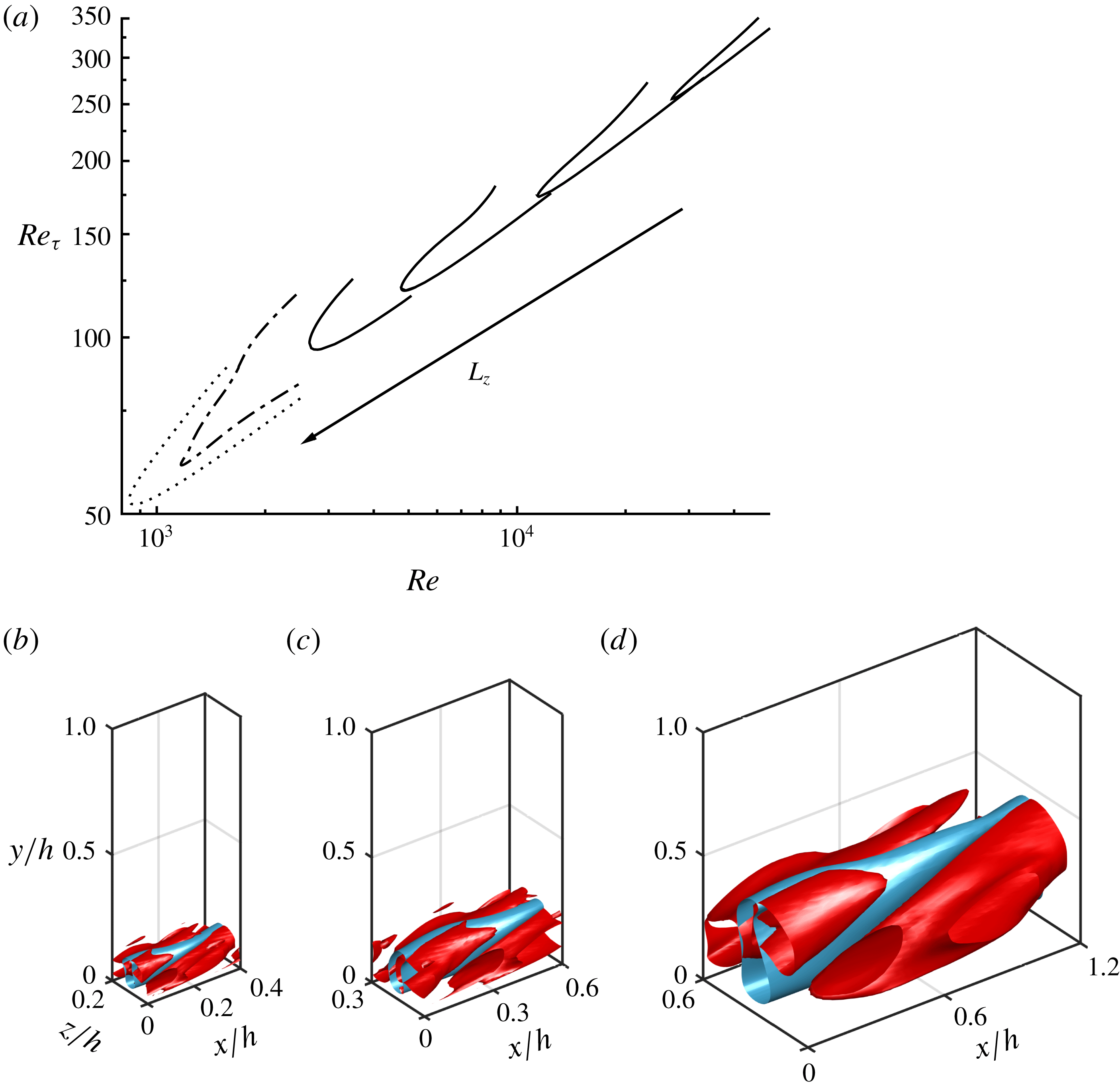
at all the domains considered. At the same time, the solutions are expected to be localised in the near-wall region (see figure 1
b–d), thereby requiring a large number of grid points in the wall-normal direction. For the solutions admitted by the Navier–Stokes equations (i.e.
 $C_{s}=0$
), two wall-normal resolutions were originally considered for the lower half-channel, i.e.
 $N_{y}=97$
and
 $N_{y}=129$
, both of which are stretched using a hyper-tangential function. These resolutions are the typical wall-normal resolutions used for direct numerical simulations at
 $Re_{\unicode[STIX]{x1D70F}}\simeq 392$
and
 $Re_{\unicode[STIX]{x1D70F}}\simeq 590$
, respectively (see e.g. Moser, Kim & Mansour Reference Moser, Kim and Mansour1999), and
 $N_{y}=97$
is found to be good enough for most of the parameters considered (see appendix A). Therefore, throughout the present study, we present the result obtained with
 $N_{y}=97$
. In the case of the solutions continued to high Reynolds number using the overdamped large-eddy simulation (i.e. with non-zero
 $C_{s}$
), the standard wall-normal resolution required for the wall-resolved large-eddy simulation at
 $Re_{\unicode[STIX]{x1D70F}}\simeq 2000$
is used for consistency with Hwang & Bengana (Reference Hwang and Bengana2016) (i.e.
 $N_{y}=65$
). We note that this relatively small number for the wall-normal resolution at such a high Reynolds number is not a great limitation, as the eddy viscosity in (2.1b
) smooths out the solution. Furthermore, the use of the eddy viscosity is introduced essentially to model the effect of surrounding turbulence, and, as such, any different kind of such models can be adopted for the same purpose. In this respect, the use of the eddy viscosity may be viewed to be ad hoc, but we shall see in § 4.2 that its use is inevitable for an energetically consistent description of coherent structures in a turbulent flow.
3 Results
3.1 Bifurcation and scaling
Bifurcation of the solutions with respect to
 $Re$
: (a) bifurcation curves for
 $L_{z}/h=0.2,~0.3,~0.45$
and
 $0.6$
; (b–d) the corresponding flow visualisations of the saddle-node points at
 $L_{z}/h=0.2,~0.3$
and
 $0.6$
, respectively. In (a), the solutions from Waleffe (Reference Waleffe2001) and Hwang et al. (Reference Hwang, Willis and Cossu2016) are presented for
 $L_{z}/h=1.5$
: – - – - –, Waleffe (Reference Waleffe2001);
 $\cdots \cdots$
, Hwang et al. (Reference Hwang, Willis and Cossu2016); ——, present study. In (b–d), the blue and red isosurfaces indicate
 ${u^{\prime }}^{+}=-2$
and
 $\unicode[STIX]{x1D706}_{2}^{+}=-0.002$
, respectively.

Bifurcation of the computed exact coherent states with
 $Re$
is reported in figure 1(a) for various spanwise domain sizes:
 $L_{z}/h=0.2,~0.3,~0.45$
and
 $0.6$
. Here,
 $Re_{\unicode[STIX]{x1D70F}}$
is defined by the friction velocity of each solution, and is introduced to the skin friction of each solution at different Reynolds numbers. In this figure, the travelling-wave solutions, previously obtained by Waleffe (Reference Waleffe2001) (dash-dotted line) and by Hwang et al. (Reference Hwang, Willis and Cossu2016) (dotted line), are reported together for
 $L_{z}=1.5h$
. We note that these previous solutions also satisfy the symmetries given by (2.2), although they are found unlikely to be connected to the family of solutions reported here (see § 3.3). For given
 $L_{z}$
, each set of the solutions shows a saddle-node bifurcation with Reynolds number: the solution that emerges at the saddle-node point divides into two, one of which becomes a high-drag state (upper branch) and the other becomes a low-drag state (lower branch). The flow structure at the onset for different
 $L_{z}$
is also shown in figure 1(b–d). It is evident that, the smaller the
 $L_{z}$
of the solution, the more localised it is to the wall. All the solutions are characterised by a ‘wavy’ streak (blue isosurfaces of streamwise velocity fluctuations) with sinuous-streak instability and streamwise vortices on the flank (red isosurfaces of the second largest eigenvalue
 $\unicode[STIX]{x1D706}_{2}$
of the symmetric tensor
 $\unicode[STIX]{x1D61A}_{ik}\unicode[STIX]{x1D61A}_{kj}+\unicode[STIX]{x1D6FA}_{ik}\unicode[STIX]{x1D6FA}_{kj}$
, where
 $\unicode[STIX]{x1D61A}_{ij}$
and
 $\unicode[STIX]{x1D6FA}_{ij}$
are the symmetric and antisymmetric parts of the velocity gradient tensor, respectively (Jeong & Hussain Reference Jeong and Hussain1995)), indicating their physical connection to the self-sustaining process.
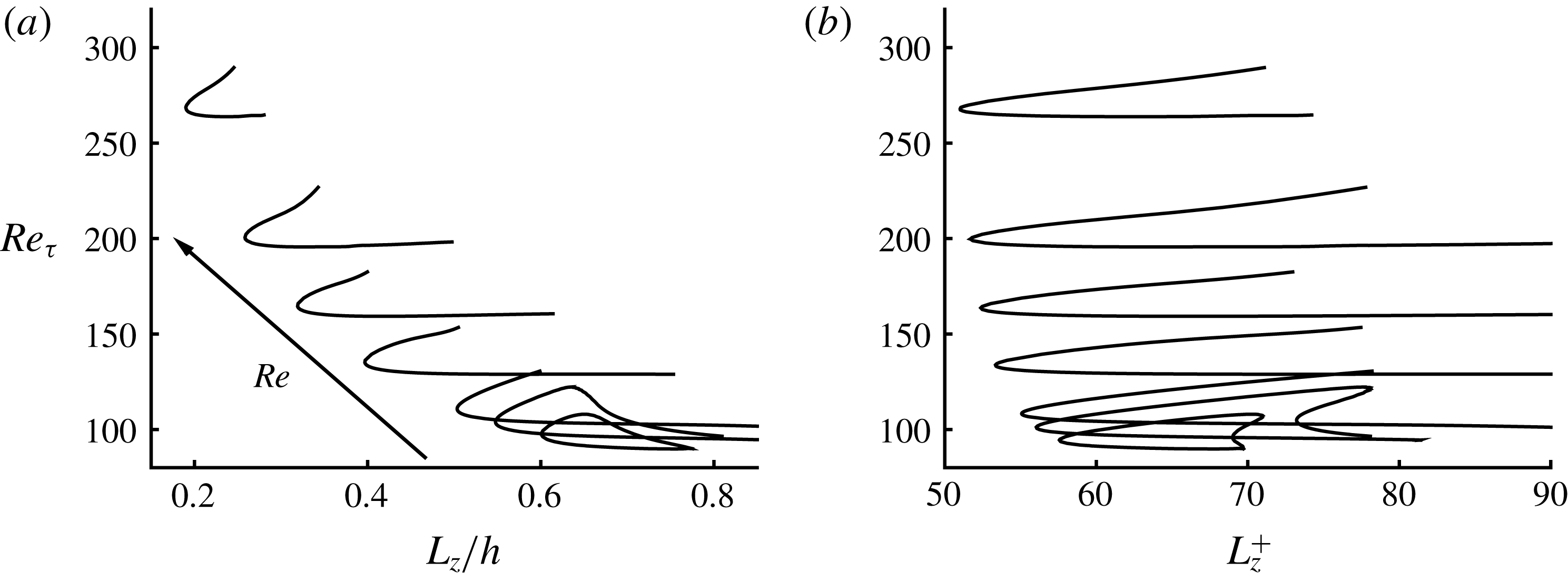
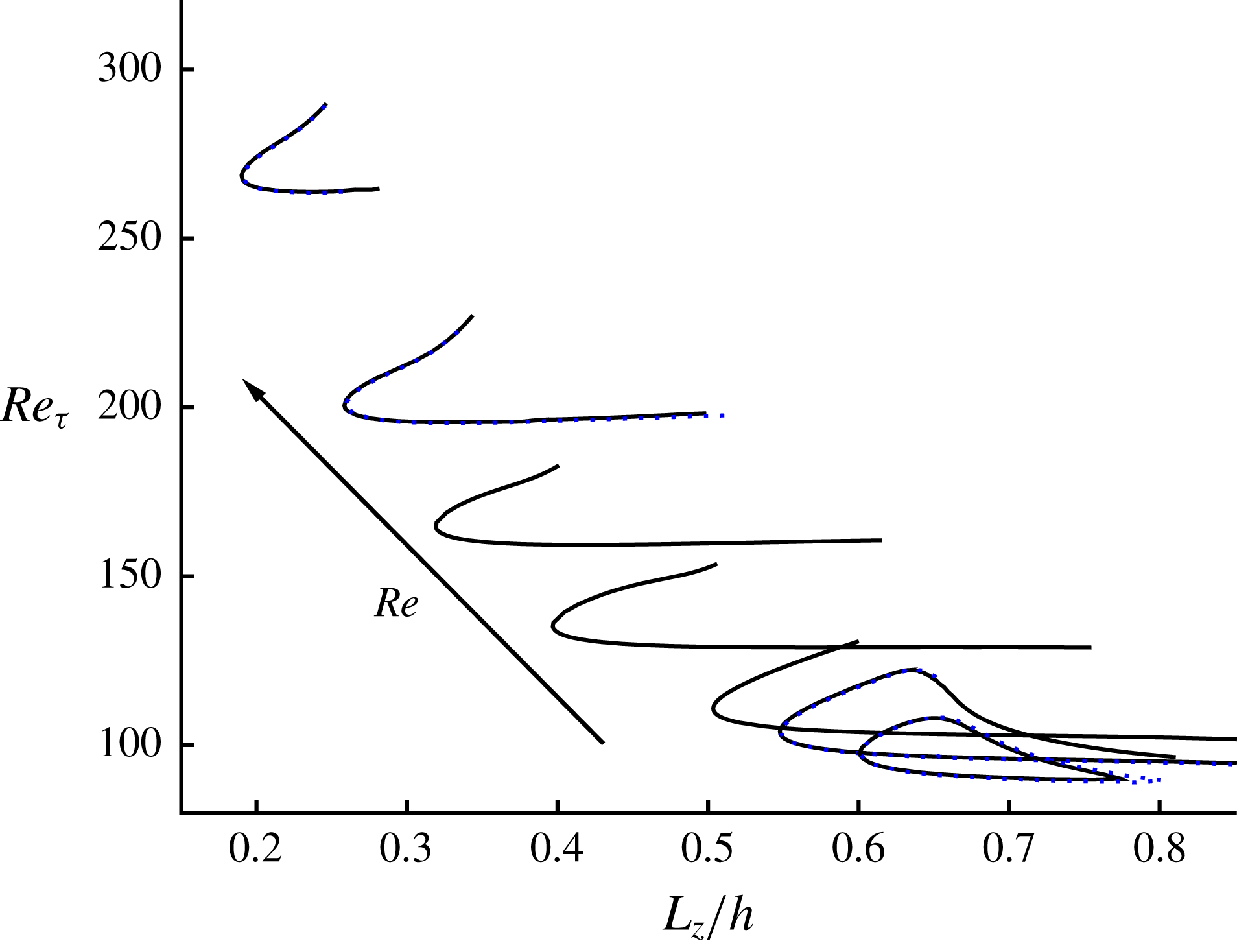
Friction Reynolds number of the solutions with respect to (a) the outer- and (b) the inner-scaled spanwise domains at
 $Re=2646,~3163,~3762,~6250,~10\,000,~15\,710$
and
 $30\,000$
.

Bifurcation of the solutions is also studied with the outer-scaled spanwise domain size
 $L_{z}/h$
, as shown in figure 2(a) for
 $Re=2646,~3163,~3762,~6250,~10\,000,~15\,710$
and
 $30\,000$
(
 $C_{s}=0$
). For each Reynolds number, the solutions emerge via a saddle-node bifurcation upon increasing
 $L_{z}$
(the left critical point of each bifurcation curve in figure 2), i.e. the solution, emerged at critical
 $L_{z}$
, is divided into the upper-branch (high-drag) and lower-branch (low-drag) states. Interestingly, in the case of the two lowest Reynolds numbers considered, these lower- and upper-branch states meet each other again, and they cannot be continued beyond a domain size greater than a certain value (
 $L_{z}/h\simeq 0.8$
for
 $Re=2646$
, and
 $L_{z}/h\simeq 0.85$
for
 $Re=3163$
). However, in general, it is not evident whether such a behaviour would also be observed for the solutions found at higher Reynolds numbers, as their continuation was found to be numerically very difficult while maintaining the relative-error tolerance of
 $10^{-6}$
in the Newton iteration.
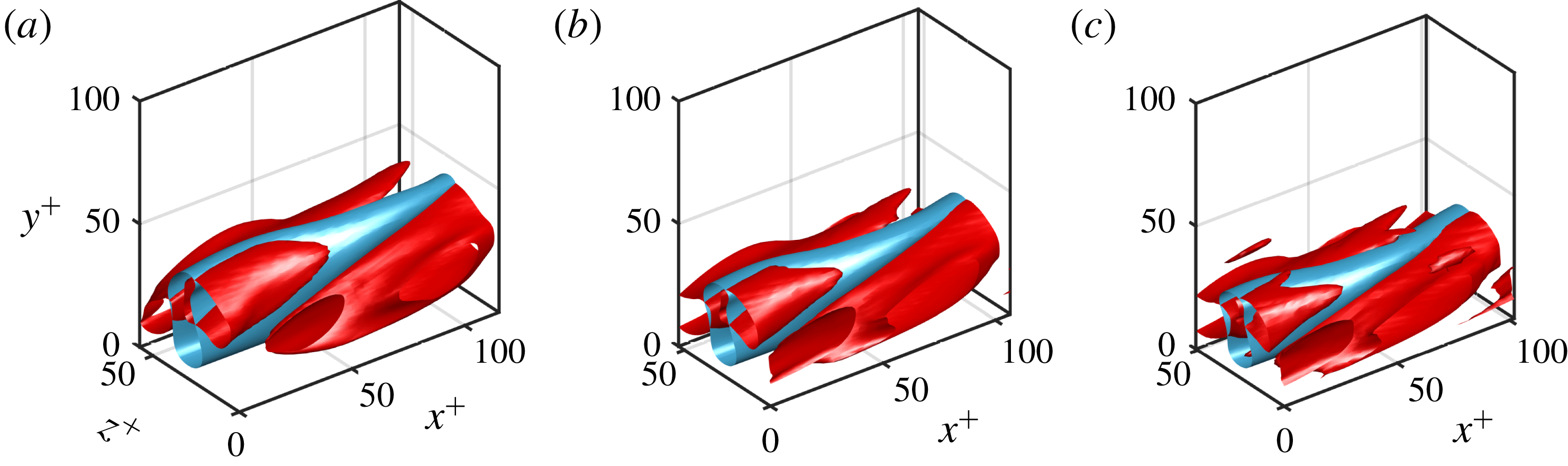
Inner-scaled flow visualisation of the solutions at the smallest
 $L_{z}^{+}$
: (a) M1, (b) M4 and (c) M7. Here, the blue and red isosurfaces indicate
 ${u^{\prime }}^{+}=-2$
and
 $\unicode[STIX]{x1D706}_{2}^{+}=-0.002$
, respectively.

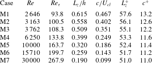
Properties of the solutions at the smallest
 $L_{z}^{+}$
in the bifurcation curve.

Inner-scaled statistics of the solutions at the smallest
 $L_{z}^{+}$
: (a)
 $U^{+}$
, (b)
 $u_{rms}^{+}$
, (c)
 $v_{rms}^{+}$
, (d)
 $w_{rms}^{+}$
, (e)
 $-\overline{u^{\prime }v^{\prime }}^{+}$
and (f)
 $-\overline{u^{\prime }v^{\prime }}^{+}(\text{d}U^{+}/\text{d}y^{+})$
. The Reynolds numbers are
 $Re=2646,~6250,~15\,710$
and
 $30\,000$
. In panel (a), the dashed line indicates
 $U^{+}=y^{+}$
.

Given the wall-localised nature of these solutions, it is also appropriate to rescale the size of these structures near the saddle-node point with viscous inner length, as presented in figure 2(b). For all Reynolds numbers considered, the smallest inner-scaled spanwise domain (
 $L_{z}^{+}=Re_{\unicode[STIX]{x1D70F}}L_{z}/h$
) of each solution is found to have similar values, although it should be noted that the saddle-node point is not defined at this domain size – the saddle-node point is defined at the minimal
 $L_{z}/h$
of the solution. The smallest inner-scaled spanwise domains at different Reynolds numbers are found to appear to approach an asymptotic value,
 $L_{z}^{+}\simeq 50$
, as
 $Re$
is increased. This is also seen in table 1, where the spanwise domain size and the phase speed of the solutions at the smallest inner-scaled spanwise domain are summarised. The smallest spanwise domain being
 $L_{z}^{+}\simeq 50$
is consistent with the typical spanwise spacing of the near-wall motions (i.e.
 $\unicode[STIX]{x1D706}_{z}^{+}\simeq 100$
) – it indicates that a chaotic state associated with the near-wall dynamics requires a spanwise size greater than
 $\unicode[STIX]{x1D706}_{z}^{+}\simeq 50$
, while typical and long-lived self-sustaining near-wall turbulence occurs for
 $L_{z}^{+}\simeq 100$
(see e.g. Jiménez & Simens Reference Jiménez and Simens2001; Hwang Reference Hwang2013). The phase speed of these solutions also approaches an asymptotic value of
 $c^{+}\simeq 11$
on increasing
 $Re$
, having the typical advection velocity (
 $c^{+}\simeq 10{-}12$
) of the near-wall coherent structures (Kim & Hussain Reference Kim and Hussain1993). The flow fields at the smallest
 $L_{z}^{+}$
of the solutions are visualised in figure 3 for three different Reynolds numbers (M1, M4 and M7 in table 1), where their domain size and levels of the flow-field isosurfaces are presented to scale in inner units. The inner-scaled solutions are very similar to each other, as is expected from the data in figure 2(b) and table 1.
One-point statistics at the smallest
 $L_{z}^{+}$
of the solutions are also examined in figure 4. To reveal the asymptotic behaviour clearer, we present the data at
 $Re=2646,~6250,~15\,710$
and
 $30\,000$
, such that their
 $Re_{\unicode[STIX]{x1D70F}}$
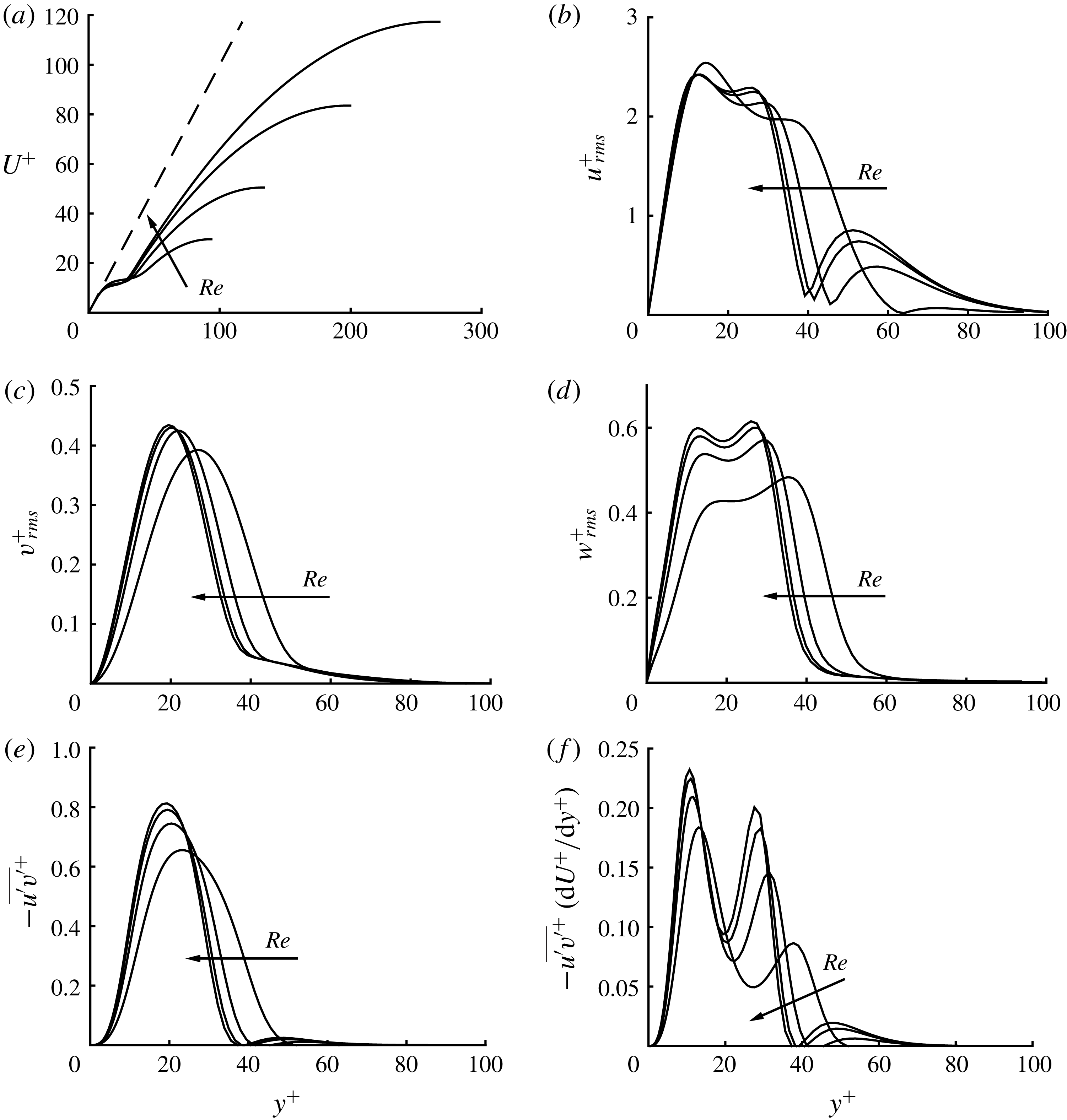
are spaced roughly in an even manner. Figure 4(a) shows the mean velocity profile, which appears to be characterised by two regions. In the region below
 $y^{+}\simeq 25$
, the mean velocity scales very well in inner units, as those in the full minimal-flow simulations (Hwang Reference Hwang2013). On the other hand, in the region above
 $y^{+}\simeq 40$
where the flow structure rarely exists, the mean flow is close to a parabola, as is the corresponding laminar base flow. Any non-trivial velocity fluctuations (figure 4
b–d), Reynolds shear stress (figure 4
e) and production (figure 4
 $f$
) appear only in the region below
 $y^{+}\simeq 40{-}60$
. In particular, those obtained from the solutions at the two highest Reynolds numbers are very close to each other, indicating that the solutions indeed approach an asymptotic state approximately independent of the Reynolds number.
In figure 4(f), it is also worth noting that turbulence production contains two peaks: one located in the region close to the wall and the other relatively further from the wall. This is not surprising, however, as this feature emerges from the fact that the present exact coherent state is an exact solution of the Navier–Stokes equations. To demonstrate this, let us consider the mean streamwise momentum equation:
 $$\begin{eqnarray}\frac{\text{d}U^{+}}{\text{d}y^{+}}-\overline{u^{\prime }v^{\prime }}^{+}=1-\frac{y^{+}}{Re_{\unicode[STIX]{x1D70F}}},\end{eqnarray}$$
where
 $\overline{\cdot }$
denotes the average in the time and the horizontal directions. In the limit of
 $Re_{\unicode[STIX]{x1D70F}}\rightarrow \infty$
, equation (3.1) indicates that the near-wall production (i.e.
 $-\overline{u^{\prime }v^{\prime }}^{+}(\text{d}U^{+}/\text{d}y^{+})$
below
 $y^{+}\simeq 50$
) should have its local maxima at the wall-normal locations where
 $-\overline{u^{\prime }v^{\prime }}^{+}=\text{d}U^{+}/\text{d}y^{+}=1/2$
. We note that
 $-\overline{u^{\prime }v^{\prime }}^{+}\simeq 1$
in the peak wall-normal location (
 $y^{+}\simeq 20$
in figure 4
e) and the present exact coherent state is localised around this location. This implies that there would be two wall-normal locations at which
 $-\overline{u^{\prime }v^{\prime }}^{+}\simeq 1/2$
if
 $Re_{\unicode[STIX]{x1D70F}}$
is sufficiently large: one appears in the region close to the wall (
 $y^{+}<20$
) and the other is located in the region further from the wall (
 $y^{+}>20$
). This is consistent with the present exact coherent state, which has two wall-normal peaks in the production: the one in the near-wall region resembles that in the turbulent state and the other originates from the wall-localised nature of the present solution.
Inner-scaled properties of the solutions for
 $Re=2646,~6250,~15\,710$
and
 $30\,000$
: (a) phase speed,
 $c^{+}$
; and peak values of (b)
 $u_{rms}^{+}$
, (c)
 $v_{rms}^{+}$
and (d)
 $-\overline{u^{\prime }v^{\prime }}^{+}$
. The arrow in each panel passes through the properties of upper-branch states.

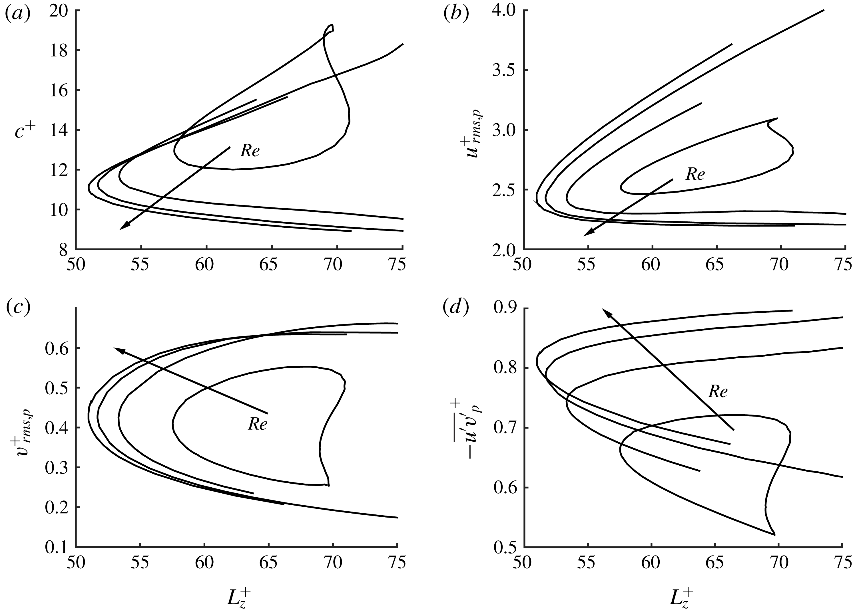
The upper- and lower-branch states are further characterised in figure 5 using the phase speed
 $c^{+}$
, the peak values of velocity fluctuations, and Reynolds shear stress for
 $Re=2646,~6250,~15\,710$
and
 $30\,000$
cases. As in figure 4, the asymptotic behaviour to a universal state is evident especially for the two highest Reynolds numbers considered. Their phase speeds are not very far from
 $c^{+}\simeq 11$
, although the ones for lower-branch states are greater than those of upper-branch ones (figure 5
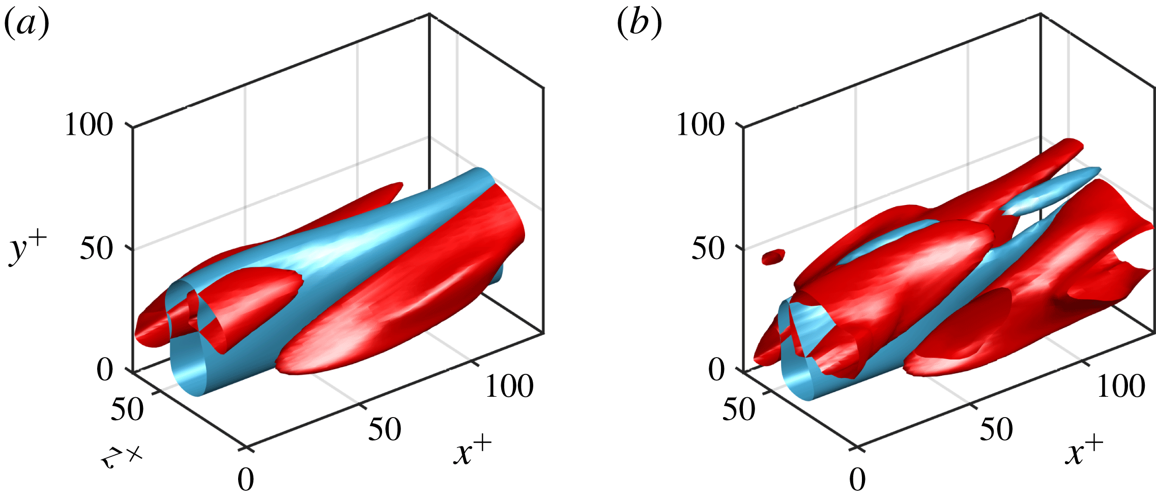
a). Similar to typical relative equilibria, the peak values of velocity fluctuations indicate that the upper-branch states feature a strong cross-streamwise velocity fluctuation, whereas the lower-branch states have a strong streamwise velocity fluctuation. The upper-branch states also contain larger Reynolds shear stress than the lower-branch ones, as is expected from the identity by Fukagata, Iwamoto & Kasagi (Reference Fukagata, Iwamoto and Kasagi2002) that directly relates Reynolds shear stress to skin-friction drag. These statistical features are also consistent with the flow fields in figure 6: the upper-branch state exhibits a strong waviness of the streak with more energetic streamwise vortices, whereas the lower-branch one consists of a relatively straight streak and weak streamwise vortices.
The stability of the solutions is examined for the smallest
 $L_{z}^{+}$
at each Reynolds number (see also figure 2
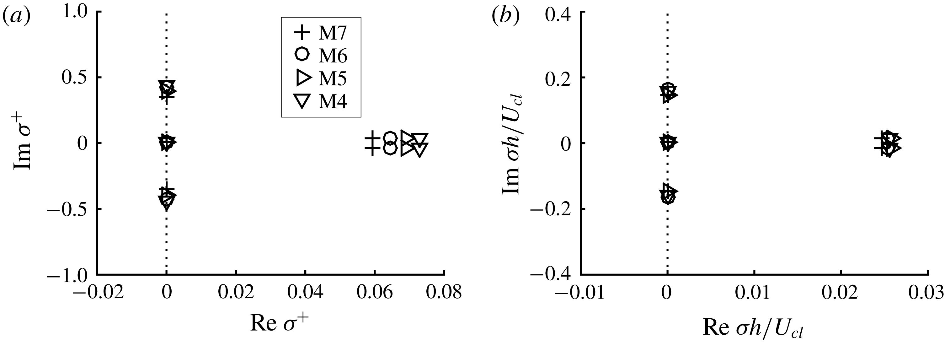
b). For this analysis, the eigenvalues of the Navier–Stokes equations linearised about the given travelling-wave solution are computed in the co-moving frame using the Arnoldi algorithm. Figure 7 shows the first five leading eigenvalues computed in the invariant subspace of (2.2). Given the fairly good inner-scaling nature of the exact coherent states, the inner scaling of the computed eigenvalues is first examined in figure 7(a). The most unstable eigenvalues of each solution appear to scale reasonably well in inner units. This feature is similar to that of the wall-localised equilibrium states (EQ7 and EQ8) in plane Couette flow (Eckhardt & Zammert Reference Eckhardt and Zammert2018), where only a few leading eigenvalues were found to scale in inner units. However, in the present channel flow, such leading eigenvalues are found to scale better with
 $U_{cl}$
and
 $h$
, as is further shown in figure 7(b). This non-intuitive behaviour needs a more careful examination of the scaling of these leading eigenvalues, and a detailed discussion on this issue will be given in § 4.1. Finally, we observe that the zero eigenvalue here is associated with the streamwise shift of the solution. The zero eigenvalue related to the saddle-node point need not quite be observed here, as the saddle-node point is defined at the minimum
 $L_{z}/h$
rather than at the minimum
 $L_{z}^{+}$
.
Flow visualisation of (a) lower- and (b) upper-branch states at
 $Re=2646$
(
 $L_{z}^{+}\simeq 65$
). Here, the blue isosurface is
 ${u^{\prime }}^{+}=-2$
, and the red isosurface is
 $\unicode[STIX]{x1D706}_{2}^{+}=-0.002$
.

Eigenspectra of the solutions at the smallest
 $L_{z}^{+}$
: (a)
 $\unicode[STIX]{x1D70E}^{+}$
and (b)
 $\unicode[STIX]{x1D70E}h/U_{cl}$
, where
 $\unicode[STIX]{x1D70E}$
denotes the eigenvalues.

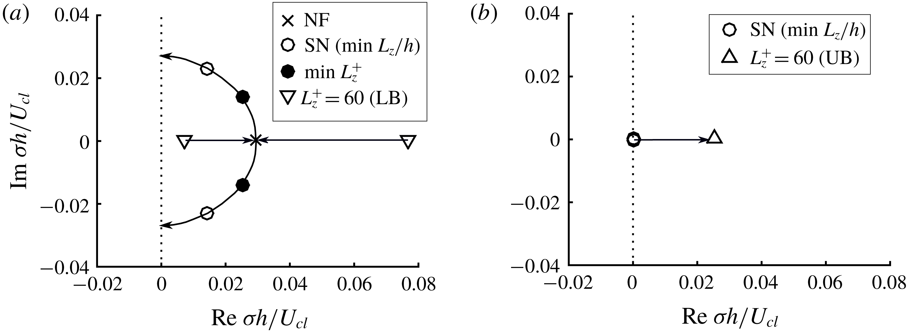
Root loci of unstable modes of the present exact coherent state at
 $Re=6250$
: (a) first two modes exhibiting a node-focus transition; (b) second mode with a single eigenvalue that becomes neutral at the saddle-node point. The arrows indicate the direction of the root loci from lower- to upper-branch state. Here, SN and NF indicate saddle-node and node-focus point, respectively.

The two unstable eigenvalues in the form of a complex conjugate pair in figure 7 indicate that the associated instability generates a modulated wave that breaks the following flow symmetry of the given solution:
 $$\begin{eqnarray}[u,v,w,p](x,y,z,t)=[u,v,w,p](x-ct,y,z,0).\end{eqnarray}$$
Focusing on
 $Re=6250$
, we further investigate the behaviour of the eigenspectra by continuing the solution in
 $L_{z}$
from the lower- to the upper-branch state. In figure 8, we present a root locus analysis by tracking a few most unstable modes with the continuation (note that the neutral eigenvalues with non-zero imaginary parts in figure 7 were not included in this analysis). The behaviour of the first type (i.e. the leading two eigenvalues in figure 7) is shown in figure 8(a). Two purely real eigenvalues in figure 7 are found to collide with each other and form a complex conjugate pair of eigenvalues, indicating a node-focus transition, as the solution is continued from the lower- to the upper-branch state. The complex conjugate pair of eigenvalues become neutral with a further continuation, indicating the formation of a limit cycle through a Hopf bifurcation. The behaviour of this mode is reminiscent of that reported for a travelling-wave solution in pipe flow (Mellibovsky & Eckhardt Reference Mellibovsky and Eckhardt2011). However, it is important to note that these eigenvalues do not cross zero at the saddle-node point (i.e. at the minimum
 $L_{z}/h$
in figure 2
a); thereby it is difficult to directly relate them to Takens–Bogdanov bifurcation. Indeed, another eigenmode is found to be related to the saddle-node bifurcation, shown in figure 8(b). This mode becomes unstable as the solution moves from the lower- to the upper-branch state. In particular, the zero crossing takes place exactly when the solution reaches the saddle node, consistent with the saddle-node bifurcation in figure 2(a).
3.2 Continuation to high Reynolds numbers
The exact coherent states discussed in the previous section are localised in the wall-normal direction, while scaling well with inner units near their critical Reynolds numbers. In this section, we will show that these states evolve into those relevant to the logarithmic region, as Reynolds number is increased. The exact solutions of the Navier–Stokes equations for
 $L_{z}/h=0.375,~0.5$
and
 $0.75$
, obtained at low Reynolds numbers (
 $Re<10\,000$
) in § 3.1, are continued to
 $Re=55\,000$
while maintaining the given
 $L_{z}$
. At this Reynolds number, the separation between the inner and the outer length scale is reasonably clear, and thus it is possible to identify physically meaningful structures associated with the logarithmic region. The three domain sizes are deliberately chosen to match the minimal attached eddies in the logarithmic region studied by Hwang & Bengana (Reference Hwang and Bengana2016). This numerical continuation is carried out while gradually increasing both
 $Re$
and
 $C_{s}$
. The target value of the Smagorinsky constant
 $C_{s}$
for each
 $L_{z}$
is chosen by carefully monitoring the one-dimensional spanwise wavenumber spectra of the corresponding overdamped simulation, such that only the largest admissible eddy survives in the given flow domain. We note that the turbulence statistics of these overdamped simulations for different
 $L_{z}$
are found to exhibit self-similarity with
 $L_{z}$
, as reported previously in Hwang (Reference Hwang2015) and Hwang & Bengana (Reference Hwang and Bengana2016) (not shown here).
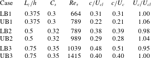
Parameters of the solutions continued to
 $Re=55\,000$
using overdamped large-eddy simulations. Here,
 $U_{c}$
denotes the centreline mean velocity of each solution.

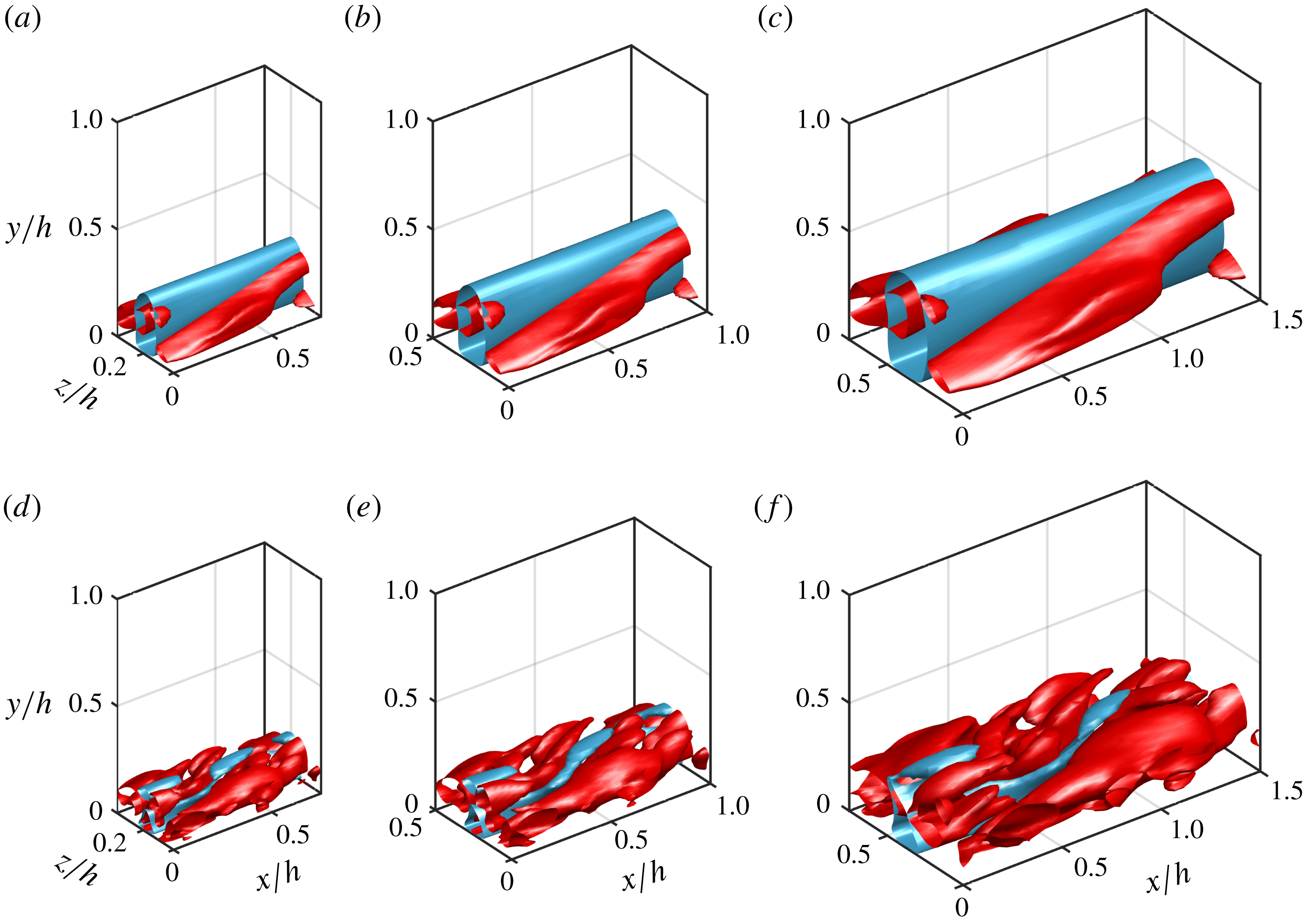
Flow visualisation of (a–c) the lower- and (d–f) the upper-branch states: (a,d)
 $L_{z}/h=0.375$
, (b,e)
 $L_{z}/h=0.5$
and (c,f)
 $L_{z}/h=0.75$
. Here, the blue isosurface indicates
 ${u^{\prime }}^{+}=-2.2$
for all the plots, while the red isosurfaces in (a–c) are
 $\unicode[STIX]{x1D706}_{2}=-5(u_{\unicode[STIX]{x1D70F}}/L_{z})^{2}$
and those in (d–f) are
 $\unicode[STIX]{x1D706}_{2}=-20(u_{\unicode[STIX]{x1D70F}}/L_{z})^{2}$
.

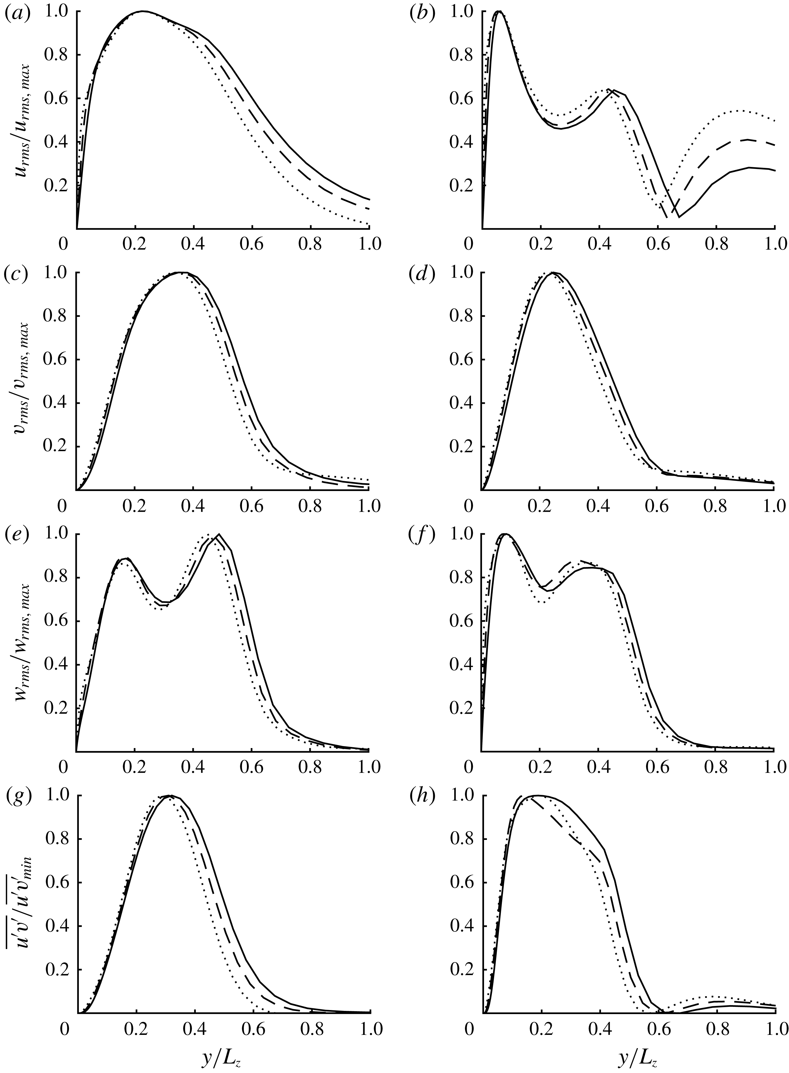
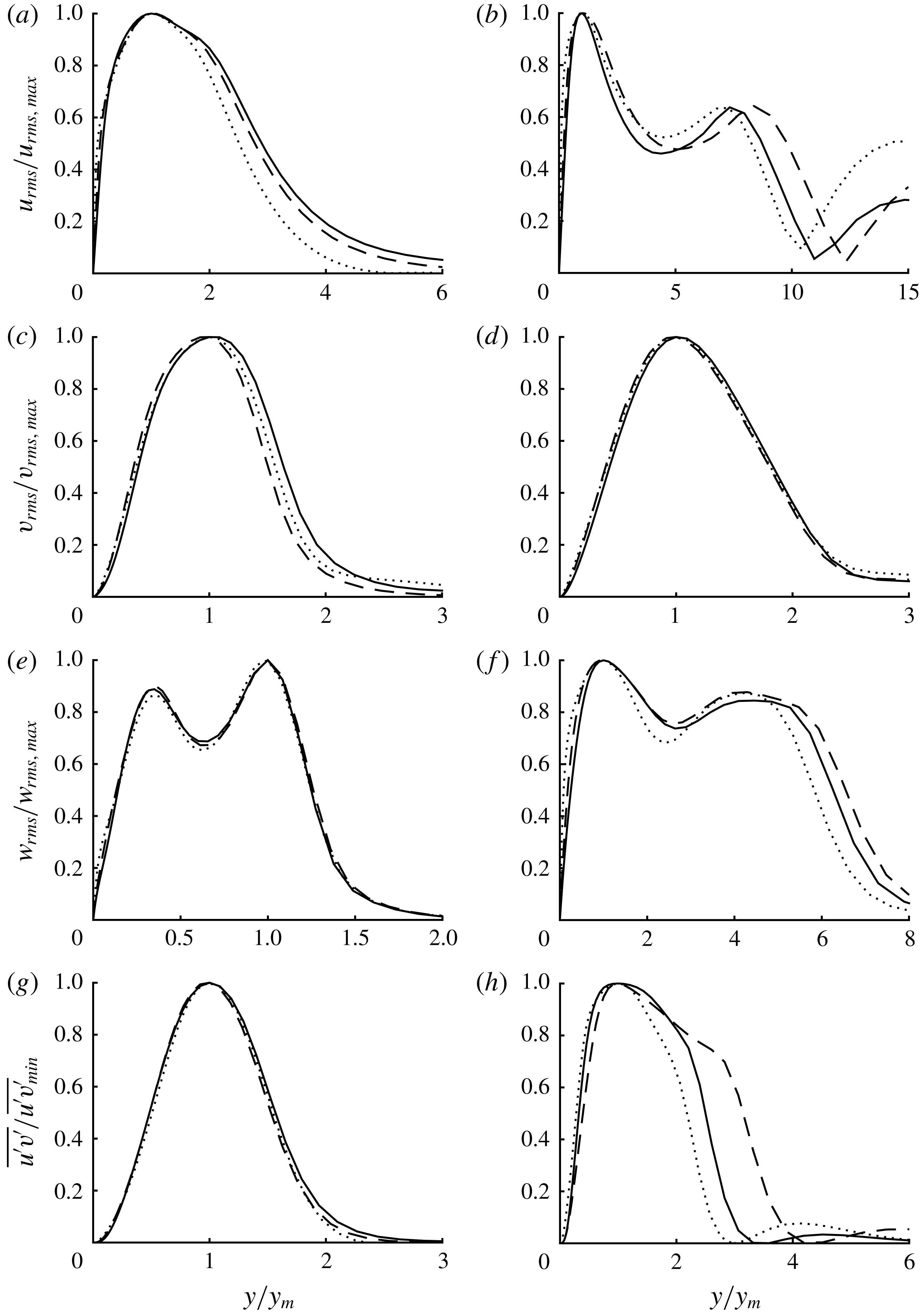
Normalised second-order statistics of (a,c,e,g) the lower- and (b,d,f,h) the upper-branch states with respect to the spanwise domain
 $L_{z}$
: (a,b) streamwise, (c,d) wall-normal, (e,f) spanwise velocity and (g,h) Reynolds shear stress. Here: ——,
 $L_{z}/h=0.375$
; – – – –,
 $L_{z}/h=0.5$
;
 $\cdots \cdots$
,
 $L_{z}/h=0.75$
.

Table 2 summarises the parameters and properties of the solutions continued to
 $Re=55\,000$
using the overdamped large-eddy simulation. Here, we note that the friction velocity of all the solutions is smaller than
 $Re_{\unicode[STIX]{x1D70F}}\simeq 1800$
, the value expected from a full simulation at this
 $Re$
for a sufficiently large computational domain (i.e.
 $L_{x}\gtrsim 3h$
and
 $L_{z}\gtrsim 1.5h$
) (de Giovanetti et al.
Reference de Giovanetti, Hwang and Choi2016). This is primarily because the contribution of the structures, the spanwise size of which is greater than the given spanwise domain
 $L_{z}$
in table 2, does not exist – see de Giovanetti et al. (Reference de Giovanetti, Hwang and Choi2016) for further details. For this reason, the friction Reynolds number of the solutions tends to be smaller on decreasing
 $L_{z}$
. Finally, the larger
 $L_{z}$
is, the larger
 $c/U_{cl}$
(or
 $c/U_{c}$
where
 $U_{c}$
is the centreline mean velocity) is found. This is expected because the solution at larger size is located further from the wall in outer units, and is thereby exposed to larger mean advection velocity. However, the mean velocity of each solution is now very different from the original one from a full simulation because the isolation procedure of the flow structures at a given spanwise length scale destroys the Reynolds shear stress carried by the structures at other length scales. Given the direct relation between Reynolds shear stress and mean velocity through the streamwise mean momentum equation (3.1), it is evident that scaling of the phase speed of the solutions would not provide any useful physical insight in relation to the original logarithmic mean velocity. Therefore, this issue has not been pursued any further.
The lower- and upper-branch solutions continued to
 $Re=55\,000$
are visualised in figure 9. The levels of the isosurfaces in this figure are scaled by
 $u_{\unicode[STIX]{x1D70F}}$
of each solution and its spanwise domain
 $L_{z}$
. The flow visualisation reveals that the flow structures of the lower- and upper-branch solutions are roughly self-similar with respect to these scales, while maintaining the typical features of exact coherent states: i.e. the upper-branch solutions contain stronger streamwise meandering motions of the streak and more intense streamwise vortical structures than the lower-branch ones.
The self-similarity of the flow structures can also be seen in the normalised turbulent velocity fluctuations and Reynolds shear stress with respect to
 $L_{z}$
, as reported in figure 10. These statistics can be scaled with the peak location of each profile, but the observed self-similarity remains almost unchanged (see appendix B). Since the upper-branch solutions will be shown to be of particular relevance to the self-sustaining turbulent state (see figures 12 and 13), here we focus mainly on statistical features of these solutions. Both the streamwise and spanwise velocity fluctuations of the upper-branch solutions have their primary peaks around the location fairly close to the wall, i.e.
 $y/L_{z}\simeq 0.06{-}0.07$
(figure 10
b,f). These velocity fluctuations are also considerably large in the region close to the wall: for example, at
 $y/L_{z}=0.05$
,
 $u_{rms}/u_{rms,max}\simeq 0.95$
and
 $w_{rms}/w_{rms,max}\simeq 0.9$
. On the other hand, the peak wall-normal locations of the wall-normal velocity fluctuation and Reynolds shear stress are located further from the wall than those of the streamwise and spanwise velocity fluctuations, i.e.
 $y/L_{z}\simeq 0.2{-}0.25$
for wall-normal velocity (figure 10
d) and
 $y/L_{z}\simeq 0.15{-}0.2$
for Reynolds shear stress (figure 10
h). Therefore, both the wall-normal velocity fluctuation and Reynolds shear stress do not reach the region close to the wall. For example, at
 $y/L_{z}=0.05$
,
 $v_{rms}/v_{rms,max}\simeq 0.2$
and
 $\overline{u^{\prime }v^{\prime }}/\overline{u^{\prime }v^{\prime }}_{min}\simeq 0.4$
, which are much smaller than those of
 $u_{rms}/u_{rms,max}$
and
 $w_{rms}/w_{rms,max}$
.
The self-similarity of the upper-branch solutions with respect to
 $L_{z}$
and their near-wall behaviour shown in figure 10 suggest that the statistical features of the upper-branch solutions are consistent with those of an ‘individual attached eddy’ in Townsend (Reference Townsend1976). Furthermore, these upper-branch solutions do appear to contribute to the logarithmic region. Since the mean velocity profile is directly coupled with Reynolds shear stress through the streamwise mean-momentum equation, this issue can be explored with the Reynolds shear-stress profile in figure 10
 $(h)$
. Note that the spanwise integral length scale in turbulent channel flow is proportional to the distance from the wall for
 $100\unicode[STIX]{x1D6FF}_{\unicode[STIX]{x1D708}}\leqslant L_{z}\leqslant 1.5h$
(e.g. Hwang Reference Hwang2015). Given the peak wall-normal location of the Reynolds shear stress profiles (i.e.
 $y/L_{z}\simeq 0.15{-}0.2$
), the wall-normal locations, to which the peak Reynolds shear stress of the upper-branch solutions contributes, would be in
 $(15{-}20)\unicode[STIX]{x1D6FF}_{\unicode[STIX]{x1D708}}\leqslant y\leqslant (0.2{-}0.3)h$
. It is evident that this range is very close to the typical wall-normal extent of the logarithmic layer, suggesting that the upper-branch solutions would indeed be relevant to the logarithmic layer.
First- and second-order statistics for
 $L_{z}/h=0.5$
: (a)
 $U^{+}$
, (b)
 $u_{rms}^{+}$
, (c)
 $v_{rms}^{+}$
and (d)
 $w_{rms}^{+}$
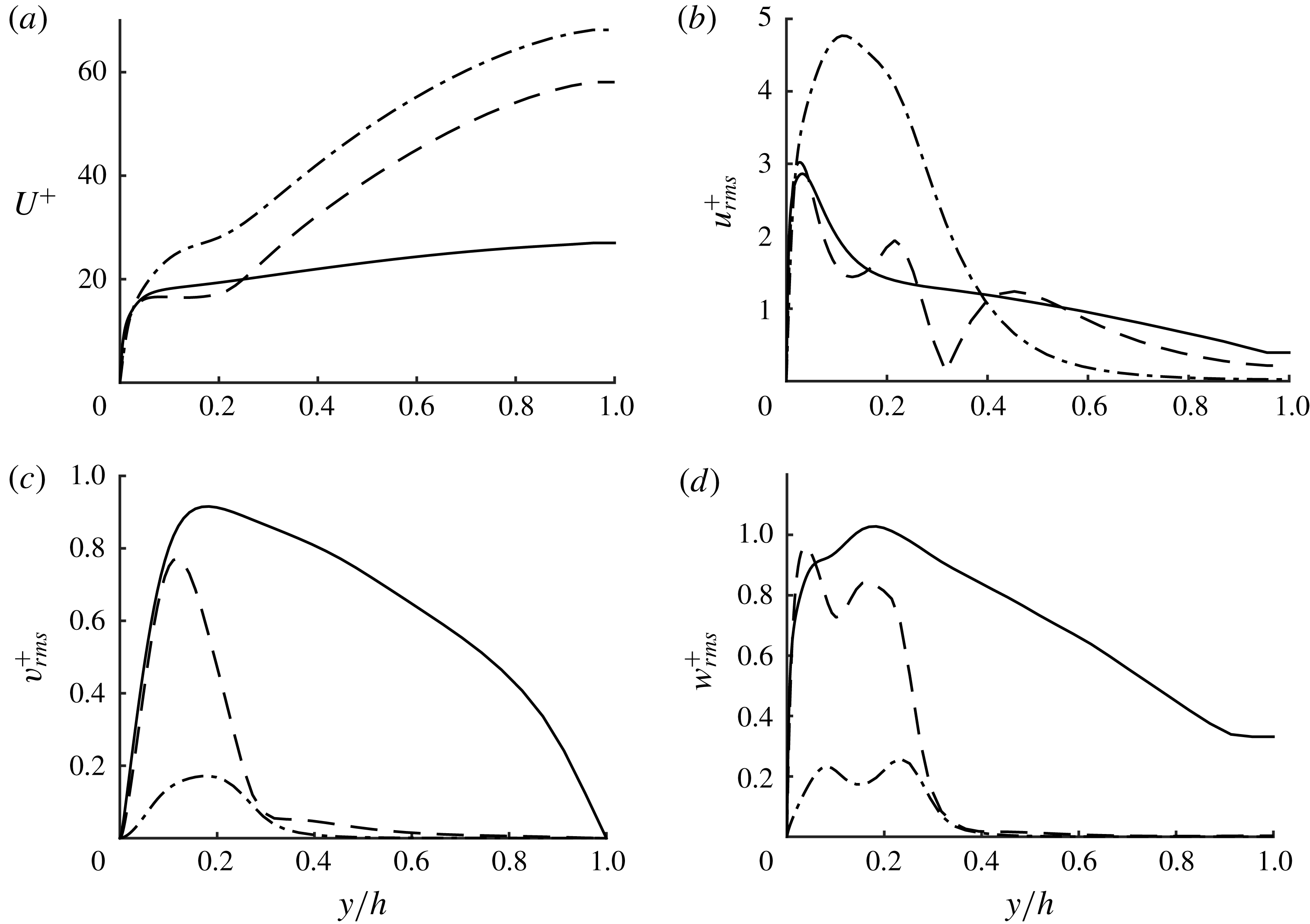
. Here: ——, full simulation; – – – –, upper-branch state (UB2); – - – - –, lower-branch state (LB2).

The observed statistical self-similarities are also consistent with the statistical data of the overdamped large-eddy simulations in Hwang (Reference Hwang2015) and Hwang & Bengana (Reference Hwang and Bengana2016). However, it is found that there is an important difference between the turbulence statistics and the present relative equilibrium states of the overdamped large-eddy simulations. Figure 11 compares first- and second-order statistics of the lower- and upper-branch solutions (LB2 and UB2) with those of the corresponding unsteady simulation for
 $L_{z}=0.5h$
at the same
 $C_{s}$
. In the region close to the wall (
 $y/h<0.2$
) where the exact coherent states carry non-zero turbulent fluctuations, the upper-branch state seems to reasonably describe the statistics of the full chaotic dynamics in the unsteady simulation. However, both upper- and lower-branch states are localised only in the region close to the wall, and, especially, their cross-streamwise velocity components carry very little energy above
 $y/h\simeq 0.2$
. This is in contrast to the full chaotic dynamics of the overdamped large-eddy simulation, because it exhibits fairly large velocity fluctuations above
 $y/h\simeq 0.2$
. It is important to mention that such non-zero turbulent fluctuations for
 $y/h>0.2$
were analysed in our recent study for minimal Couette flow (Yang, Willis & Hwang Reference Yang, Willis and Hwang2018), and they were shown to be the consequence of local mean shear in such an outer region, which admits self-sustaining processes at the length scale of the artificially narrow spanwise domain.
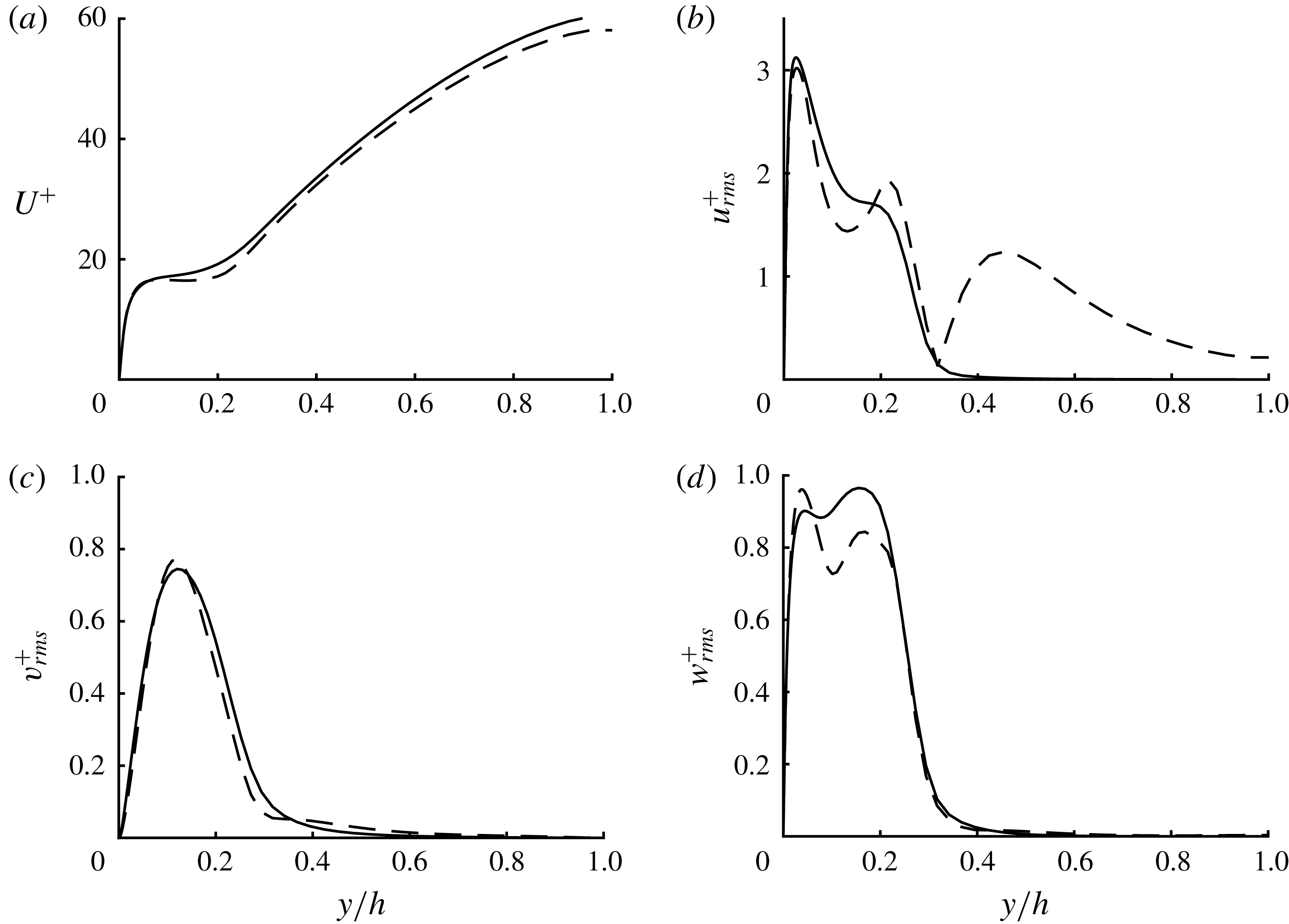
First- and second-order statistics for
 $L_{z}/h=0.5$
: (a)
 $U^{+}$
, (b)
 $u_{rms}^{+}$
, (c)
 $v_{rms}^{+}$
and(d)
 $w_{rms}^{+}$
. Here: ——, simulation with damping (3.3); – – – –, upper-branch state (UB2).

Towards isolating the chaotic dynamics associated mainly with the solutions in the present study, we perform an additional numerical simulation, in which the velocity fluctuations above a certain wall-normal location are artificially damped out. Note that this technique is similar to the one used in Jiménez & Pinelli (Reference Jiménez and Pinelli1999). We consider the following form of body forcing to the right-hand side of the Navier–Stokes equations:
 $$\begin{eqnarray}f_{i}=\unicode[STIX]{x1D707}(y)(u_{i}-\langle u_{i}\rangle _{x,z}),\end{eqnarray}$$
where
 $\langle \cdot \rangle _{x,z}$
indicates the average in the streamwise and spanwise directions and
 $$\begin{eqnarray}\unicode[STIX]{x1D707}(y)=\unicode[STIX]{x1D707}_{0}\left\{1-\frac{1}{2}\left[1+\tanh \left(10\left(\frac{\unicode[STIX]{x1D702}^{2}}{\unicode[STIX]{x1D702}_{0}^{2}}-1\right)\right)\right]\right\}.\end{eqnarray}$$
Here,
 $\unicode[STIX]{x1D707}_{0}~(=U_{cl}/h)$
is the damping strength used,
 $\unicode[STIX]{x1D702}=y/h-1$
,
 $\unicode[STIX]{x1D702}_{0}=y_{0}/h-1$
, and
 $y_{0}$
is the wall-normal location, above which the damping (3.3) is applied. The location of
 $y_{0}$
is determined by gradually lowering from the centreline until turbulence is not sustained in the domain; this gives
 $y_{0}=0.6L_{z}$
. Figure 12 compares the first- and second-order statistics of the upper-branch state (UB2) with those of an overdamped simulation with (3.3) (
 $y_{0}=0.3h$
) for
 $L_{z}/h=0.5$
. It is evident that the statistics now compare much more favourably with each other (compare figure 12 with figure 11), indicating the upper-branch state as a good proxy of the self-sustaining energy-containing motion below
 $y/h\simeq 0.3$
.
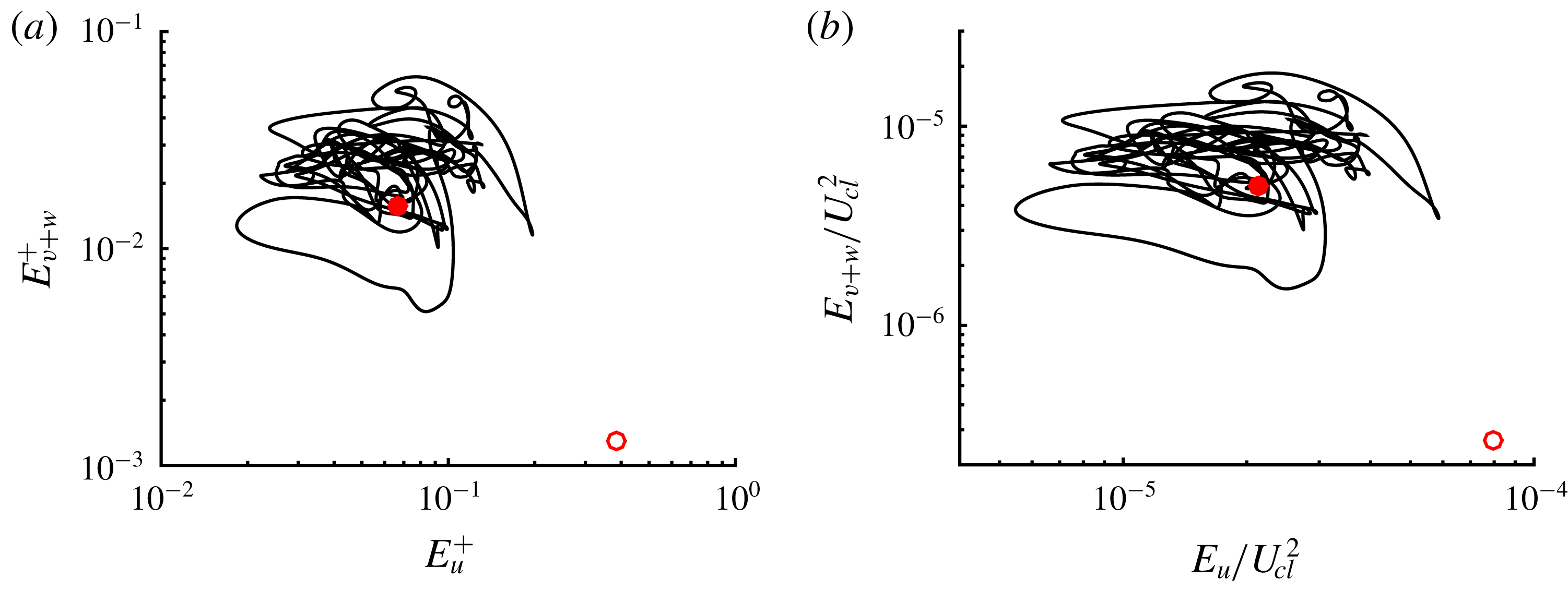
Phase portrait for
 $L_{z}/h=0.5$
in the plane of
 $E_{u}$
–
 $E_{v+w}$
scaled in (a) inner and (b) outer units. Here: ——, simulation with damping (3.3); open circles, LB2; and filled circles, UB2.

From the simulation with the damping function (3.3), the state-space location of the upper-branch state can be shown. To this end, we consider the following state-space variables:
 $$\begin{eqnarray}E_{u}=\frac{1}{2V_{\unicode[STIX]{x1D6FA}_{n}}}\int _{\unicode[STIX]{x1D6FA}_{n}}{u^{\prime }}^{2}\,\text{d}V,\quad E_{v+w}=\frac{1}{2V_{\unicode[STIX]{x1D6FA}_{n}}}\int _{\unicode[STIX]{x1D6FA}_{n}}{v^{\prime }}^{2}+{w^{\prime }}^{2}\,\text{d}V,\end{eqnarray}$$
where
 $u^{\prime }$
,
 $v^{\prime }$
and
 $w^{\prime }$
are streamwise, wall-normal and spanwise velocity fluctuations, respectively. Here,
 $V_{\unicode[STIX]{x1D6FA}_{n}}$
is the volume of the near-wall region of the computational domain defined as
 $\unicode[STIX]{x1D6FA}_{n}=[0,L_{x}]\times [0,0.6L_{z}]\times [0,L_{z}]$
, and this is introduced to consider only the region where both the damped simulation and the solutions continued with the eddy viscosity carry non-negligibly large velocity fluctuations (note that energy input and dissipation have not been considered as the dissipation of the damped simulation requires incorporation of the contribution from the damping body force in (3.3), whereas the solutions do not). In figure 13, the phase portraits respectively scaled by
 $u_{\unicode[STIX]{x1D70F}}$
and
 $U_{cl}$
in the
 $E_{u}$
–
 $E_{v+w}$
plane are shown. In both cases, the upper-branch state is reasonably well placed in the middle of the chaotic solution trajectory given by the self-sustaining motion at the given size, suggesting that the upper-branch state would be a reasonable proxy for the near-wall chaotic dynamics and its skin-friction generation in the damped simulation.
3.3 Relation to other solutions
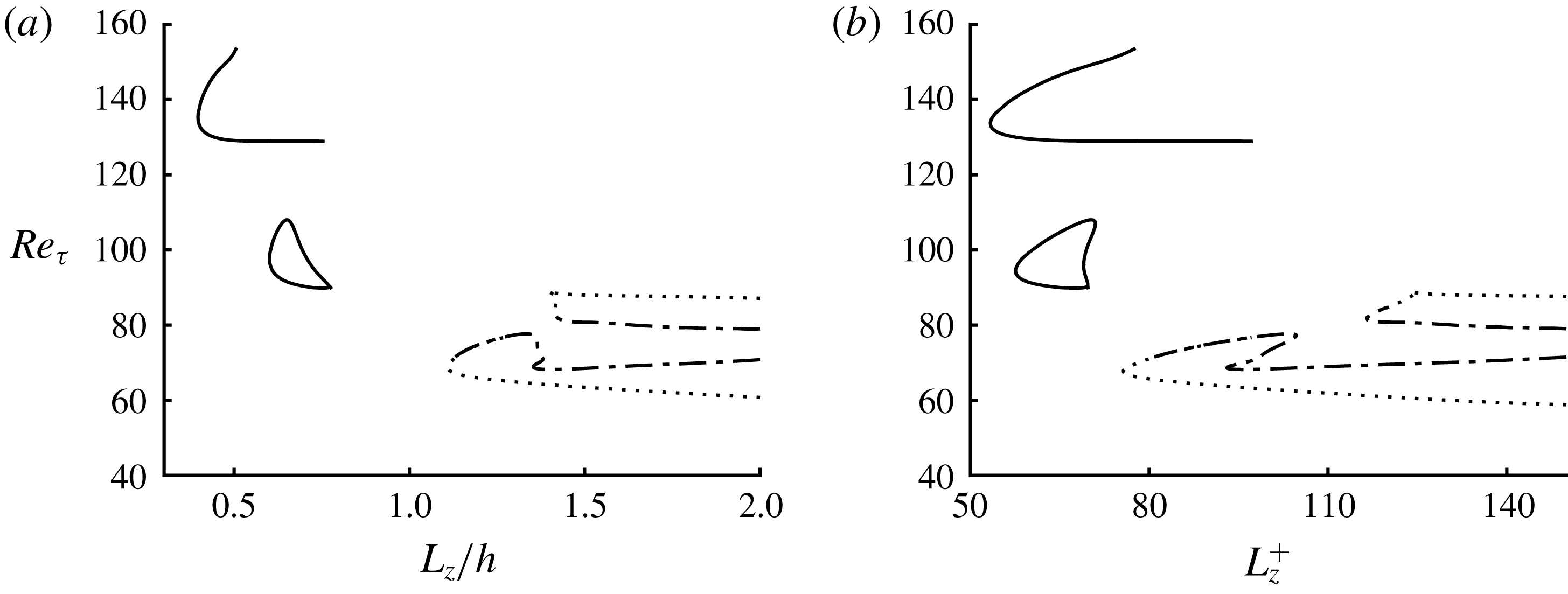
(a) Outer- and (b) inner-scaled bifurcation curves with
 $L_{z}$
. Here: – - – - –, Waleffe (Reference Waleffe2001) and
 $\cdots \cdots$
, Hwang et al. (Reference Hwang, Willis and Cossu2016) at
 $Re=1538$
; whereas ——, at
 $Re=2646$
(lower curve) and
 $Re=6250$
(upper curve).

The relative equilibrium states in the present study belong to the invariant subspace described by (2.2). The two solutions previously reported by Waleffe (Reference Waleffe2001) and Hwang et al. (Reference Hwang, Willis and Cossu2016) also belong to this subspace, although they were computed in different ways: the solution in Waleffe (Reference Waleffe2001) was obtained by continuously deforming the base flow from the one of Nagata (Reference Nagata1990) in plane Couette flow, whereas the solution in Hwang et al. (Reference Hwang, Willis and Cossu2016) was obtained using an overdamped large-eddy simulation designed to isolate self-sustaining large- and very-large-scale motions, the spanwise size of which is
 $L_{z}/h\simeq 1.5$
(Hwang & Cossu Reference Hwang and Cossu2010b
). In this section, we explore whether the solutions in the present study have any link with these previous solutions. It is useful to remember that the solutions reported in the present study could be continued only for small spanwise domain (
 $L_{z}/h\lesssim 1$
; see also figure 2), whereas those in Waleffe (Reference Waleffe2001) and Hwang et al. (Reference Hwang, Willis and Cossu2016) were previously reported for the spanwise domains larger than
 $L_{z}/h\simeq 1$
.
First, numerical continuation of the solutions in Waleffe (Reference Waleffe2001) and in Hwang et al. (Reference Hwang, Willis and Cossu2016) is performed by gradually lowering
 $L_{z}$
. Here, the solution of Waleffe (Reference Waleffe2001) was obtained by downloading its raw data from his personal webpage. His solution was interpolated onto our grid system, then used as initial condition of our Newton solver. The Newton iteration converged quickly and the retrieved solution using our solver showed excellent agreement with that in Waleffe (Reference Waleffe2001). The continuation result of the two pairs of the solutions in Waleffe (Reference Waleffe2001) and in Hwang et al. (Reference Hwang, Willis and Cossu2016) with
 $L_{z}$
is shown in figure 14 at
 $Re=1538$
. For a sufficiently large spanwise domain (
 $L_{z}/h>1.5$
or
 $L_{z}^{+}>140$
), the two solution pairs form four equilibrium states. As
 $L_{z}$
is decreased, their upper-branch states meet each other around
 $L_{z}/h\simeq 1.4$
(
 $L_{z}^{+}\simeq 120$
) and the lower-branch ones exhibit the same behaviour around
 $L_{z}/h\simeq 1.2$
(
 $L_{z}^{+}\simeq 75$
). This suggests that the solutions in Waleffe (Reference Waleffe2001) and in Hwang et al. (Reference Hwang, Willis and Cossu2016) are homotopic relatives, while implying that they are unlikely to be continued for
 $L_{z}\lesssim h$
. Furthermore, these solutions are found not to be localised in the near-wall region, as
 $L_{z}$
is decreased (not shown here).
By contrast, it is found that the solutions in the present study begin to emerge at a little higher Reynolds number (see the solid line curves at
 $Re=2646$
in figure 14). This suggests that the solutions in the present study are unlikely to be continuously or directly linked to those reported in Waleffe (Reference Waleffe2001) and Hwang et al. (Reference Hwang, Willis and Cossu2016). However, any possibility of their mutual connections should not be completely ignored at this moment. Indeed, the disappearance of the solutions of Waleffe (Reference Waleffe2001) and Hwang et al. (Reference Hwang, Willis and Cossu2016) on decreasing
 $L_{z}$
might be linked to the emergence of different types of invariant solutions, such as a relative periodic orbit, through a saddle-node infinite period (SNIPER) bifurcation, as was recently reported in Rawat, Cossu & Rincon (Reference Rawat, Cossu and Rincon2016) with the solution of Waleffe (Reference Waleffe2001) for large
 $L_{z}({>}2h)$
at
 $Re=2000$
. Such a periodic orbit emerging from the SNIPER bifurcation might be connected to the solutions in the present study, although pursuing this issue any further is beyond the scope of the present study.
Finally, the present solutions are compared with those recently reported by Eckhardt & Zammert (Reference Eckhardt and Zammert2018) in plane Couette flow. We note that the wall-localised solutions in Eckhardt & Zammert (Reference Eckhardt and Zammert2018) originate from a pair of the solutions (EQ7 and EQ8) in Gibson et al. (Reference Gibson, Halcrow and Cvitanovic2009), and they are obtained by rescaling the Navier–Stokes equations with its spanwise domain size using the uniform base-flow shear of plane Coutte flow. While their solutions were found to scale in inner units as those in the present study, it appears that their spatial structure is significantly different from the present solutions in plane channel flow. For example, the EQ7 and EQ8 solutions in Gibson et al. (Reference Gibson, Halcrow and Cvitanovic2009) typically exhibit two pairs of streaks and quasi-streamwise vortices, and the high- and low-speed streaks alternate along the streamwise directions. By contrast, the spatial structure of the present solution features a pair of high- and low-speed streaks continuously linked along the streamwise direction (figure 6), which is more like the solutions found in Waleffe (Reference Waleffe2001) and Hwang et al. (Reference Hwang, Willis and Cossu2016). This suggests that the solutions in the present study are not likely to be homotopic with those in Eckhardt & Zammert (Reference Eckhardt and Zammert2018).
4 Discussion
4.1 Scaling of the exact coherent states
The exact coherent states in the present study have been found to scale approximately in inner units, except their eigenvalues, which appear to scale better with the time scale of the laminar base flow (figure 7 b). Given the wall-localised nature of these states, this observation is intuitively unexpected, leading us to examine their precise scaling more carefully. To address this issue, it is instructive to consider the equation for the rate of the total kinetic energy per unit volume:
 $$\begin{eqnarray}\frac{\text{d}E}{\text{d}t}=I-D,\end{eqnarray}$$
where
 $$\begin{eqnarray}\displaystyle \left.\begin{array}{@{}c@{}}\displaystyle E=\frac{1}{2V_{\unicode[STIX]{x1D6FA}}}\int _{\unicode[STIX]{x1D6FA}}u_{i}u_{i}\,\text{d}V,\\ \displaystyle I=\frac{U_{m}\unicode[STIX]{x1D708}}{V_{\unicode[STIX]{x1D6FA}}}\int _{0}^{L_{x}}\int _{0}^{L_{z}}\frac{\unicode[STIX]{x2202}u}{\unicode[STIX]{x2202}y}\Bigg|_{y=0}\,\text{d}x\,\text{d}z,\quad D=\frac{\unicode[STIX]{x1D708}}{V_{\unicode[STIX]{x1D6FA}}}\int _{\unicode[STIX]{x1D6FA}}\frac{\unicode[STIX]{x2202}u_{i}}{\unicode[STIX]{x2202}x_{j}}\frac{\unicode[STIX]{x2202}u_{i}}{\unicode[STIX]{x2202}x_{j}}\,\text{d}V.\end{array}\right\} & & \displaystyle\end{eqnarray}$$
Here,
 $V_{\unicode[STIX]{x1D6FA}}~(=L_{x}\times L_{y}\times L_{z})$
is the volume of the computational domain
 $\unicode[STIX]{x1D6FA}$
,
 $I$
the rate of energy input originating from the applied pressure gradient,
 $D$
the rate of dissipation, and
 $U_{m}~(=(2/3)U_{cl})$
the bulk velocity. We first restrict ourselves to the relative equilibrium solutions in the present study. From (4.1), it is evident that the rate of energy input for the given equilibrium state is
 $I=(U_{m}/h)u_{\unicode[STIX]{x1D70F}}^{2}$
. Unless the dissipation mechanism imposes different velocity and time scales, the velocity scale of the kinetic energy
 $E$
should become
 $u_{\unicode[STIX]{x1D70F}}$
with the evolution time scale given by
 $T_{e}=h/U_{m}$
. This is expected to be particularly true near the critical Reynolds number at which the solutions emerge, because their integral and dissipation scales are expected to be hardly separated. Indeed, at the saddle-node point of the solutions, we have shown that the velocity fluctuations scale well with
 $u_{\unicode[STIX]{x1D70F}}$
(e.g. figure 5) and that the leading eigenvalues in figure 7 scale well with
 $T_{e}$
(equivalently to
 $h/U_{cl}$
with the factor
 $3/2$
).
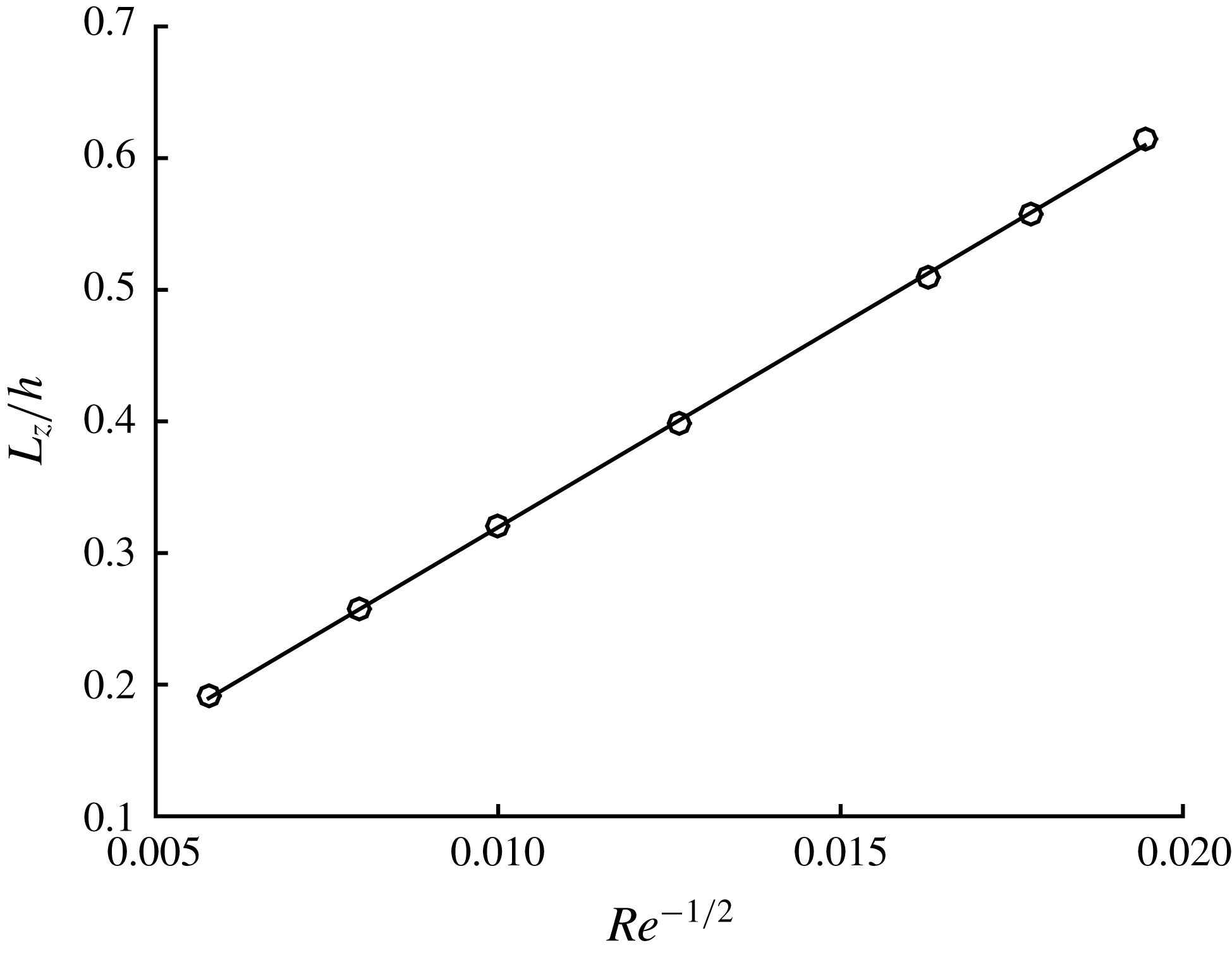
Scaling of the critical spanwise domain
 $L_{z}$
at the onset of the exact coherent states with respect to
 $Re^{-1/2}$
.

At first glance, this observation, made with (4.1) and figure 7(b), is seemingly odd because
 $T_{e}$
is the time scale of fluid motion which travels downstream with the ‘bulk’ velocity
 $U_{m}$
over the ‘outer’-scaling distance
 $h$
. Indeed, it is intuitively difficult to imagine how any wall-localised fluid motion, such as the solutions in the present study, would scale with such a global time scale
 $T_{e}$
instead of the local viscous inner time scale
 $T_{in}=\unicode[STIX]{x1D708}/u_{\unicode[STIX]{x1D70F}}^{2}$
. However, there is also further evidence supporting
 $T_{e}$
as the time scale of the solutions in the present study. Given the expected little scale separation between the processes of
 $I$
and
 $D$
near the saddle-node point of the solutions, the rate of dissipation in this case would scale as
 $D\sim \unicode[STIX]{x1D708}u_{\unicode[STIX]{x1D70F}}^{2}/L_{z}^{2}$
(
 $L_{z}$
is the spanwise size of the solutions). The balance between
 $I$
and
 $D$
in (4.1) with
 $\text{d}E/\text{d}t=0$
yields the following scaling of the spanwise wavelength with Reynolds number:
 $$\begin{eqnarray}\frac{L_{z}}{h}\sim \frac{1}{\sqrt{Re}},\end{eqnarray}$$
providing scaling of the saddle-node point of the exact coherent states in the ‘outer unit’. Here, we note again that (4.2) is obtained by setting
 $I=u_{\unicode[STIX]{x1D70F}}^{2}/T_{e}$
. In figure 15, (4.2) is examined by plotting the spanwise domain size of each solution at the saddle-node point as a function of
 $1/\sqrt{Re}$
. It is evident that (4.2) provides an excellent prediction for the ‘outer’ scaling of the spanwise domain size of the saddle-node point with Reynolds number, suggesting that
 $T_{e}$
would indeed be the time scale of the present exact coherent states.
All of the observations, made on the time scale of the present exact coherent states, are physically difficult to explain, unless there exists an explicit mathematical relation between
 $T_{e}$
and
 $T_{in}$
. Therefore, we now explore how they are precisely related to each other for the solutions in the present study. In the limit of
 $Re\rightarrow \infty$
, the size of the solutions have been shown to asymptotically scale in inner units (i.e.
 $L_{z}^{+}\simeq \text{const.}$
, as shown in table 1. Combining this with (4.2) then yields
 $$\begin{eqnarray}\frac{u_{\unicode[STIX]{x1D70F}}}{U_{cl}}\sim \frac{1}{\sqrt{Re}}\quad \text{and}\quad \frac{\unicode[STIX]{x1D6FF}_{\unicode[STIX]{x1D708}}}{h}\sim \frac{1}{\sqrt{Re}},\end{eqnarray}$$
which provide the explicit relation between the inner scales and those of the laminar base flow. It is then straightforward to realise
 $$\begin{eqnarray}T_{e}\sim T_{in},\end{eqnarray}$$
indicating that
 $T_{in}$
is actually proportional to
 $T_{e}$
for
 $Re\rightarrow \infty$
. This now explains that
 $T_{in}$
would be the time scale for the solutions, if
 $Re\rightarrow \infty$
, and confirms that the relatively poor inner scaling of the eigenvalues in figure 7(a) is the finite-Reynolds-number effect of the solutions.
Based on this observation, we now take
 $u_{\unicode[STIX]{x1D70F}}$
and
 $T_{in}$
as the velocity and time scales, and consider
 $Re\rightarrow \infty$
. Then, in this limit, we have that the mean and velocity fluctuations of the exact coherent states in the present study are governed by the following equations:
 $$\begin{eqnarray}\frac{\text{d}U^{+}}{\text{d}y^{+}}-\overline{(u^{\prime }v^{\prime })}^{+}=1,\end{eqnarray}$$
 $$\begin{eqnarray}\frac{\unicode[STIX]{x2202}{u_{i}^{\prime }}^{+}}{\unicode[STIX]{x2202}t^{+}}+U_{j}^{+}\frac{\unicode[STIX]{x2202}{u_{i}^{\prime }}^{+}}{\unicode[STIX]{x2202}x_{j}^{+}}+{u_{j}^{\prime }}^{+}\frac{\unicode[STIX]{x2202}U_{i}^{+}}{\unicode[STIX]{x2202}x_{j}^{+}}=-\frac{\unicode[STIX]{x2202}{p^{\prime }}^{+}}{\unicode[STIX]{x2202}x_{i}^{+}}+\frac{\unicode[STIX]{x2202}^{2}{u_{i}^{\prime }}^{+}}{\unicode[STIX]{x2202}x_{j}^{+}\unicode[STIX]{x2202}x_{j}^{+}}-{u_{j}^{\prime }}^{+}\frac{\unicode[STIX]{x2202}{u_{i}^{\prime }}^{+}}{\unicode[STIX]{x2202}x_{j}^{+}}+\overline{{u_{j}^{\prime }}^{+}\frac{\unicode[STIX]{x2202}{u_{i}^{\prime }}^{+}}{\unicode[STIX]{x2202}x_{j}^{+}}},\end{eqnarray}$$
 $U_{i}=U(y)\unicode[STIX]{x1D6FF}_{i1}$
is the mean velocity, and
 $u_{i}^{\prime }$
and
 $p^{\prime }$
are the velocity and pressure fluctuations, respectively. Here the mean equation (4.5a
) now explicitly excludes the term originating from the mean pressure gradient because
 $Re_{\unicode[STIX]{x1D70F}}\rightarrow \infty$
from (4.3): indeed, if the Reynolds shear stress is zero, (4.5a
) indicates that the base flow becomes a uniform shear flow, as one would easily expect.
Equations (4.5) now suggest that different types of wall-localised exact coherent states can be further sought using (4.5) rather than the full equations. This would be particularly beneficial from the computational viewpoint, since these exact coherent states do not contain any significant flow structures in most of the wall-normal domain. Furthermore, the viscous term in (4.5) is given at the order of unity, suggesting that such solutions at least at their onset would follow the asymptotic description proposed by Deguchi (Reference Deguchi2015) with imposition of a no-slip boundary condition at the wall. Finally, the form of the mean equation (4.5a
) indicates that the full turbulent dynamics of (4.5) is also relevant to description of the dynamics of the so-called ‘mesolayer’, in which the effect of viscous force from the presence of the wall dominates over that of the pressure gradient. Given the size of the mesolayer scaling as
 $\unicode[STIX]{x0394}y^{+}\sim \sqrt{Re_{\unicode[STIX]{x1D70F}}}$
(where
 $\unicode[STIX]{x0394}y^{+}$
is the wall-normal extent of the mesolayer (see Afzal Reference Afzal1982; Sreenivasan & Sahay Reference Sreenivasan, Sahay and Panton1997)), the only additional requirement should be that the size of the computational domain needs to follow
 $L_{dom}\ll \sqrt{Re_{\unicode[STIX]{x1D70F}}}$
, where
 $L_{dom}$
is the size of computational domain in all the directions.
4.2 Continuation to high Reynolds numbers with eddy viscosity
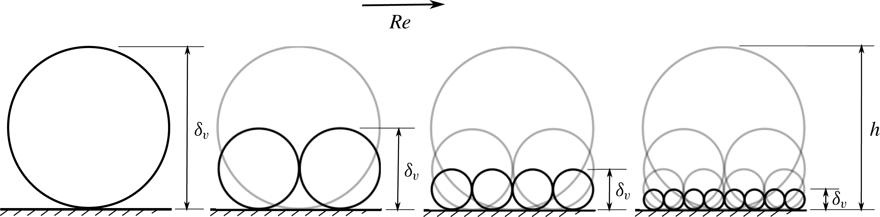
The continuation of the exact coherent states to high Reynolds number in § 3.2 has been carried out by introducing an eddy viscosity, which was implemented using the overdamped large-eddy simulation (e.g. Hwang & Cossu Reference Hwang and Cossu2010b ). Introduction of such an artificially elevated eddy viscosity was originally done to examine the self-sustaining processes in the logarithmic and outer regions. However, in the present study, its main benefit lies in enabling us to extend the dynamical systems notions to high Reynolds numbers. In particular, it technically relaxes the numerical difficulty typically arising in continuation of the upper-branch states to high Reynolds numbers, which are highly relevant to the description of the turbulent state. To provide a more comprehensive discussion of the physical relevance of the present eddy-viscosity-based approach, we start by considering the dimensional form of the equations for turbulent fluctuation. Since the size of the coherent structures in fully developed turbulence and the present exact coherent states is well characterised by the spanwise length scale (e.g. Hwang Reference Hwang2015), it is useful to consider a Fourier-mode decomposition of turbulent velocity fluctuation in the spanwise direction:
 $$\begin{eqnarray}u_{i}^{\prime }(t,x,y,z)=\int _{-\infty }^{\infty }\widehat{u_{i}^{\prime }}(t,x,y;k_{z})\text{e}^{\text{i}k_{z}z}\,\text{d}k_{z},\end{eqnarray}$$
where
 $\widehat{\cdot }\;$
denotes the Fourier-transformed state and
 $k_{z}$
is the spanwise wavenumber. Then, the streamwise-averaged equation for the turbulent kinetic energy at each spanwise wavenumber (i.e.
 $\widehat{e}(y;k_{z})=\widehat{u_{i}^{\prime }}(y;k_{z})\widehat{u_{i}^{\prime }}^{\ast }(y;k_{z})$
) is given by
 $$\begin{eqnarray}\displaystyle \overline{\frac{\unicode[STIX]{x2202}\widehat{e}(y;k_{z})}{\unicode[STIX]{x2202}t}} & = & \displaystyle \underbrace{\left\langle \text{Re}\left\{-\overline{\widehat{u^{\prime }}^{\ast }(y;k_{z})\widehat{v^{\prime }}(y;k_{z})}\hspace{2.22198pt}\frac{\text{d}U(y)}{\text{d}y}\right\}\right\rangle _{x}}_{\widehat{P}(y;k_{z})}+\underbrace{\left\langle -\unicode[STIX]{x1D708}\overline{\frac{\unicode[STIX]{x2202}\widehat{u_{i}^{\prime }}(y;k_{z})}{\unicode[STIX]{x2202}x_{j}}\frac{\unicode[STIX]{x2202}\widehat{u_{i}^{\prime }}^{\ast }(y;k_{z})}{\unicode[STIX]{x2202}x_{j}}}\hspace{2.22198pt}\right\rangle _{x}}_{\widehat{\unicode[STIX]{x1D700}}(y;k_{z})}\nonumber\\ \displaystyle & & \displaystyle +\underbrace{\left\langle \text{Re}\left\{-\overline{\widehat{u_{i}^{\prime }}^{\ast }(y;k_{z})\frac{\unicode[STIX]{x2202}}{\unicode[STIX]{x2202}x_{j}}\left(\widehat{u_{i}^{\prime }u_{j}^{\prime }}(y;k_{z})\right)}\hspace{2.22198pt}\right\}\right\rangle _{x}}_{\widehat{T}_{turb}(y;k_{z})}\nonumber\\ \displaystyle & & \displaystyle +\underbrace{\left\langle \text{Re}\left\{\frac{\text{d}}{\text{d}y}\left(-\overline{\frac{\widehat{p^{\prime }}(y;k_{z})\widehat{v^{\prime }}^{\ast }(k_{z})}{\unicode[STIX]{x1D70C}}}\hspace{2.22198pt}\right)\right\}\right\rangle _{x}}_{\widehat{T}_{p}(y;k_{z})}+\underbrace{\left\langle \unicode[STIX]{x1D708}\frac{\text{d}^{2}\,\overline{\widehat{e}(y;k_{z})}}{\text{d}y^{2}}\hspace{2.22198pt}\right\rangle _{x}}_{\widehat{T}_{\unicode[STIX]{x1D708}}(y;k_{z})},\end{eqnarray}$$
where
 $^{\ast }$
denotes the complex conjugate, and
 $\langle \hspace{2.22198pt}\cdot \hspace{2.22198pt}\rangle _{x}$
the spatial average in the
 $x$
-direction. Here,
 $\widehat{P}(y;k_{z})$
is turbulence production,
 $\widehat{\unicode[STIX]{x1D700}}(y;k_{z})$
dissipation,
 $\widehat{T}_{turb}(y;k_{z})$
nonlinear turbulent transport,
 $\widehat{T}_{p}(y;k_{z})$
transport by pressure, and
 $\widehat{T}_{\unicode[STIX]{x1D708}}(y;k_{z})$
viscous transport (i.e. diffusion of turbulent kinetic energy). In the region above the wall,
 $\widehat{T}_{p}(y;k_{z})$
and
 $\widehat{T}_{\unicode[STIX]{x1D708}}(y;k_{z})$
have been found to be negligible, and they will be excluded in the following discussion on the energetics of coherent structures in the logarithmic region. Also,
 $\unicode[STIX]{x2202}\widehat{e}(y;k_{z})/\unicode[STIX]{x2202}t$
goes to zero with the time average. For a further discussion on these issues, the reader may refer to Cho, Hwang & Choi (Reference Cho, Hwang and Choi2018) and Lee & Moser (Reference Lee and Moser2019).
Given the scale of turbulent kinetic energy in (4.2) and the logarithmic mean velocity, turbulence production should scale as
 $\widehat{P}(y;k_{z,int})\sim u_{\unicode[STIX]{x1D70F}}^{3}/y$
at the wavenumbers of integral length scales (
 $k_{z,int}\sim 2\unicode[STIX]{x03C0}/y$
) where turbulence production mainly takes place and dissipation is negligibly small. Therefore, from (4.7), the main energy balance at
 $k_{z}=k_{z,int}$
is given by
 $$\begin{eqnarray}\widehat{P}(y;k_{z,int})+\widehat{T}_{turb}(y;k_{z,int})\simeq 0,\end{eqnarray}$$
as numerically confirmed by, for example, Cho et al. (Reference Cho, Hwang and Choi2018). This balance can also be checked by scaling the nonlinear turbulent transport term with the integral velocity and length scales in the logarithmic region (i.e.
 $u_{\unicode[STIX]{x1D70F}}$
and
 $y$
):
 $\widehat{T}_{turb}(y;k_{z,int})\sim O(u_{\unicode[STIX]{x1D70F}}^{3}/y)$
, whereas
 $\widehat{\unicode[STIX]{x1D700}}(y;k_{z,int})\sim O(Re_{y}^{-1}u_{\unicode[STIX]{x1D70F}}^{3}/y)$
with
 $Re_{y}~(=u_{\unicode[STIX]{x1D70F}}y/\unicode[STIX]{x1D708})\rightarrow \infty$
by the definition of the logarithmic layer. Therefore, for
 $k=k_{int}$
, the dissipation
 $\widehat{\unicode[STIX]{x1D700}}$
cannot be balanced with the production
 $\widehat{P}$
, and the only possible way to form the energy balance is through (4.8).
Since turbulent transport is an energy-preserving process over the given computational domain,
 $\int _{-\infty }^{\infty }\widehat{T}_{turb}(y;k_{z})\,\text{d}k_{z}\simeq 0$
in the logarithmic layer (Cho et al.
Reference Cho, Hwang and Choi2018). This implies that the negative
 $\widehat{T}_{turb}(y;k_{z,int})$
in (4.8) should be positive at some other
 $k_{z}$
. It is evident that this process should take place through energy cascade to dissipate out the produced turbulent kinetic energy. The dissipation process takes place at the Kolmogorov microscale given by
 $\unicode[STIX]{x1D702}\equiv (\unicode[STIX]{x1D708}^{3}/\widehat{P}(y;k_{z,int}))^{1/4}$
, thus
 $\unicode[STIX]{x1D702}\sim y^{1/4}$
in the logarithmic region. Since turbulence production at the dissipation scales should be negligibly small, the main energy balance at the dissipation length scale (i.e.
 $k=k_{z,dis}~({\sim}2\unicode[STIX]{x03C0}/\unicode[STIX]{x1D702})$
) is given by
 $$\begin{eqnarray}\widehat{T}_{turb}(y;k_{z,dis})+\widehat{\unicode[STIX]{x1D700}}(y;k_{z,dis})\simeq 0.\end{eqnarray}$$
Here, (4.9) is made by approximating the energy-conservative nature of nonlinear turbulent transport (i.e.
 $\int _{-\infty }^{\infty }\widehat{T}_{turb}(y;k_{z})\,\text{d}k_{z}\!\simeq 0$
), such that
 $\widehat{T}_{turb}(y;k_{z,dis})+\widehat{T}_{turb}(y;k_{z,int})\simeq 0$
. From (4.8), one can easily derive
 $$\begin{eqnarray}\widehat{P}(y;k_{z,int})\simeq \widehat{\unicode[STIX]{x1D700}}(y;k_{z,dis}),\end{eqnarray}$$
the balance between turbulence production and dissipation in the logarithmic layer (Tennekes & Lumley Reference Tennekes and Lumley1967), which is also consistent with the spectral budget analysis of full numerical simulation data in Cho et al. (Reference Cho, Hwang and Choi2018) and Lee & Moser (Reference Lee and Moser2019).
Now, let us consider the overdamped large-eddy simulations, in which all the motions, except the self-sustaining one at
 $k_{z}=k_{z,int}$
, are damped out by artificially increasing
 $C_{s}$
in (2.1). It is evident that this artificial elimination of the motions at other scales would significantly reduce the role of nonlinear transport in (4.8), as there are now very few motions to nonlinearly interact with each other. However, the physical dissipation at the integral length scale (i.e.
 $\widehat{\unicode[STIX]{x1D700}}(y;k_{z,int})$
) cannot be large at high Reynolds numbers, indicating that the dissipation by the artificially elevated eddy viscosity is replacing the role of
 $\widehat{T}_{turb}(y;k_{z,int})$
, such that
 $$\begin{eqnarray}\widehat{P}(y;k_{z,int})+\widehat{\unicode[STIX]{x1D716}}_{\unicode[STIX]{x1D708}}(y;k_{z,int})\simeq 0,\end{eqnarray}$$
where
 $\widehat{\unicode[STIX]{x1D716}}_{\unicode[STIX]{x1D708}}(y;k_{z,int})$
is the dissipation by the eddy-viscosity model in (2.1). Here, it is important to mention that the replacement of
 $\widehat{T}_{turb}(y;k_{z,int})$
with
 $\widehat{\unicode[STIX]{x1D716}}_{\unicode[STIX]{x1D708}}(y;k_{z,int})$
should not change at least the value of
 $\widehat{P}(y;k_{z,int})$
. In other words, the friction velocity
 $u_{\unicode[STIX]{x1D70F}}$
should be maintained to be roughly the same in this replacement process, since
 $\widehat{P}(y;k_{z,int})\sim u_{\unicode[STIX]{x1D70F}}^{3}/y$
. Indeed, the use of (2.1) has been consistently found not to yield any significant change in the friction velocity (see e.g. Hwang Reference Hwang2015), indicating that it does not significantly modify the value of
 $\widehat{P}(y;k_{z,int})$
described by the self-sustaining process and the exact coherent states in the present study. By contrast, an artificial elevation molecular viscosity (i.e. lowering Reynolds number) significantly reduces
 $\widehat{P}(y;k_{z,int})$
as well, because it also involves a significant reduction of the friction velocity.
A schematic illustration of the evolution of attached eddies in turbulent channel flow. Dark circles indicate attached eddies at the emergence, and grey circles indicate attached eddies evolved from those at lower Reynolds numbers.

The discussion here suggests that modelling the surrounding turbulence using an eddy-viscosity-based model, as in the present study, provides an energetically consistent description for the processes at high Reynolds numbers, although it is essentially ad hoc to extend the notions of dynamical systems to such regimes. Given this nature, it is also possible to consider any other form of such a model as long as it correctly models the energetics described here. In this respect, it is finally worth mentioning the recent phenomenological modelling of coherent structures using the notions of the relative equilibrium (Chini et al. Reference Chini, Montemuro, White and Klewicki2017), and such a modelling effort may also take some benefit from the energy balance discussed here.
5 Concluding remarks
We have presented a family of exact coherent states, individual members of which appears to underpin the individual attached eddy hypothesised by Townsend (Reference Townsend1976). The initial condition for the Newton iteration in the present study was obtained from an overdamped large-eddy simulation with a narrow spanwise computational domain, in which the related energy-containing eddies reside through their self-sustaining process (Hwang & Bengana Reference Hwang and Bengana2016). Then, a converged exact coherent state of the Navier–Stokes equations was obtained, and the solution family was subsequently calculated by continuing with the spanwise domain size and with Reynolds number. It has been found that these solutions emerge with a scaling in inner units, suggesting that, right after the onset (i.e. the saddle-node point), they underpin the self-sustaining process of near-wall coherent structures. Continuation of these solutions to high Reynolds number, using the overdamped large-eddy simulation (Hwang & Cossu Reference Hwang and Cossu2010b ; Hwang Reference Hwang2015), has further revealed that they evolve into the self-similar states in the logarithmic region, each of which underpins the self-sustaining process at its length scale.
This observation for the exact coherent states in the present study indicates that the near-wall region (say
 $y^{+}\leqslant 30$
) is the location where new sets of coherent structures are born on increasing Reynolds number, and their size scales in inner units near this onset. With further increase of Reynolds number, the near-wall structure that emerged at different (lower) Reynolds numbers subsequently evolves into the structures in the logarithmic region at different length scales, as illustrated by the schematic in figure 16. It is evident that this process leads the main flow topology in the logarithmic region to become in the form of a hierarchy of self-similar coherent structures, consistent with the attached eddy hypothesis of Townsend (Reference Townsend1976). From this perspective, the self-similarity of the coherent structures in the logarithmic region is a natural consequence of this process, as they all initially emerged in the form of near-wall coherent structures at lower Reynolds numbers.
The invariant solutions of the Navier–Stokes equations found in the present study provide solid evidence on the existence of Townsend’s attached eddies, each of which would underpin the self-sustaining process of an individual attached eddy at a given length scale. The present result also provides direct support for the previous work conducted with the linearised Navier–Stokes equations where self-similar linear transient-growth/resolvent/proper orthogonal decomposition modes were found (del Álamo & Jiménez Reference del Álamo and Jiménez2006; Hwang & Cossu Reference Hwang and Cossu2010a ; Moarref et al. Reference Moarref, Sharma, Tropp and McKeon2013). Finally, it is tempting to use the statistics of the present exact coherent states as the input for the previous analysis based on linear superposition of statistics of individual attached eddies (e.g. Perry, Henbest & Chong Reference Perry, Henbest and Chong1986; Perry & Marusic Reference Perry and Marusic1995). However, it should be pointed out that the Navier–Stokes equations are nonlinear. Therefore, in principle, such a superposition, which would strictly be valid for the linearly decomposable statistics of the given flow (e.g. Fourier modes), is not feasible with the present solutions, placing a new challenge for a theoretical description of high-Reynolds-number turbulence using invariant solutions. Nevertheless, bifurcation of these states in the present study has provided important physical insight into the fundamental mechanism by which the hierarchical organisation of self-similar coherent structures is formed throughout the logarithmic layer on increasing Reynolds numbers.
Acknowledgements
Q.Y. would like to acknowledge the National Key Research and Development Program of China (2016YFA0401200) and the Natural Science Foundation of China (11802322, 11772350, 11702307). Y.H. was supported by the Engineering and Physical Sciences Research Council (EPSRC) in the UK (EP/N019342/1).
Appendix A. Effect of wall-normal resolution
The effect of wall-normal resolution is shown in figure 17, where the bifurcation diagram with
 $L_{z}$
is shown for
 $N_{y}=97$
and
 $N_{y}=129$
. It appears that the use of
 $N_{y}=97$
shows excellent agreement with that of
 $N_{y}=129$
, only except around
 $L_{z}/h\simeq 0.8$
.
Friction Reynolds number of the solutions with respect to the outer spanwise domains at
 $Re=2646,~3163,~3762,~6250,~10\,000,~15\,710$
and
 $30\,000$
: here: ——,
 $N_{y}=97$
; – – – –,
 $N_{y}=129$
.

Normalised second-order statistics of (a,c,e,g) the lower- and (b,d,f,h) the upper-branch states with respect to the peak location of each profile,
 $y_{m}$
: (a,b) streamwise, (c,d) wall-normal and (e,f) spanwise velocity and (g,h) Reynolds shear stress. Here: ——,
 $L_{z}/h=0.375$
; – – – –,
 $L_{z}/h=0.5$
;
 $\cdots \cdots$
,
 $L_{z}/h=0.75$
.

Appendix B. Effect of reference length scale for attached eddies
In Townsend’s attached eddy hypothesis (Townsend Reference Townsend1956, Reference Townsend1976), the length scale of each attached eddy is the distance from its centre to the wall (i.e.
 $y$
). Hwang (Reference Hwang2015) has shown that the spanwise size of the attached eddy is proportional to its centre height. Therefore, in the present study, the spanwise domain
 $L_{z}$
has been used as the reference length scale, as shown in figure 10. However, the self-similarity in figure 10 remains almost unchanged if the statistics of the present exact solution of the overdamped simulation are rescaled with the distance from the wall. To demonstrate this, the normalised second-order statistics for the lower- and upper-branch states in figure 10 are scaled with the peak wall-normal location of each profile,
 $y_{m}$
, and they are shown in figure 18. Reasonably good self-similarity is also observed as in figure 10.