1 Introduction
The settling of small solid particles in either gaseous or liquid flows with density stratification is a topic of great interest in fluid dynamics. Such multi-phase flows are widely encountered in nature. An example is the settling of small aggregates of organic matter, ‘marine snow’, in the ocean (Van Aartrijk & Clercx Reference Van Aartrijk and Clercx2010; Guasto, Rusconi & Stocker Reference Guasto, Rusconi and Stocker2012; De Pietro et al. Reference De Pietro, van Hinsberg, Biferale, Clercx, Perlekar and Toschi2015; Sozza et al. Reference Sozza, De Lillo, Musacchio and Boffetta2016). Here density stratification is due to either salt concentration or temperature gradients. A second example is the dynamics of pollutants in the atmosphere which is often stably stratified turbulence (Jacobson Reference Jacobson2005; Leelőssy et al. Reference Leelőssy, Molnár, Izsák, Havasi, Lagzi and Mészáros2014). It is important to understand the settling speed of particles in such flows, because it determines their residence times and deposition rates. Also, density-stratified fluids occur in industrial processes that involve heated fluids (Linden Reference Linden1999), or the mixing of fluids of different densities (Turner Reference Turner1979).
To compute, from first principles, the drag force experienced by the particles as they fall through the flow is a difficult problem, in particular if there is turbulence. Many authors have therefore concentrated on particle dynamics in quiescent stratified fluids. Settling through a sharp density interface was measured in experiments (Srdić-Mitrović, Mohamed & Fernando Reference Srdić-Mitrović, Mohamed and Fernando1999; Abaid et al. Reference Abaid, Adalsteinsson, Agyapong and Mclaughlin2004; Camassa et al. Reference Camassa, Falcon, Lin, Mclaughlin and Parker2009) and in simulations (Blanchette & Shapiro Reference Blanchette and Shapiro2012; Ardekani, Doostmohammadi & Desai Reference Ardekani, Doostmohammadi and Desai2017; Pierson & Magnaudet Reference Pierson and Magnaudet2018). Direct numerical simulation (DNS) studies of particles settling in quiescent, linearly stratified fluids were reported by Torres et al. (Reference Torres, Hanazaki, Ochoa, Castillo and Van Woert2000), Yick et al. (Reference Yick, Torres, Peacock and Stocker2009), Ardekani & Stocker (Reference Ardekani and Stocker2010). Stratification can significantly slow down the settling particle by enhancing the drag it experiences (Yick et al. Reference Yick, Torres, Peacock and Stocker2009). The reason is that buoyancy differences due to the stratification tend to prevent the vertical motion of the fluid that the particle stirs up as it settles. As a consequence, the disturbance flow remains confined around the particle (Ardekani & Stocker Reference Ardekani and Stocker2010). How much the particle is slowed down depends on the mechanisms that govern the dynamics of the fluid density: diffusion of concentration or temperature, their advection by the disturbance flow or a combination of diffusion and advection.
Which of these mechanisms is most important depends on the physical system in question. In salt water, for example, the diffusion coefficient of salt is much smaller than the kinematic viscosity of the fluid. Therefore salt water is often considered non-diffusive. But when temperature comes into play this may not be a good approximation, because the diffusion coefficient of temperature in water is roughly of the same order as the kinematic viscosity. This is even more important in gases where the temperature diffusion coefficient may exceed the kinematic viscosity of the fluid (Salazar Reference Salazar2003).
The nature of the disturbance flow caused by the settling particle depends on how efficiently the fluid disturbance is convected away. This is an inertial effect. So stratification, diffusion and convective fluid inertia compete to determine the drag force on the particle. When the convective fluid-inertia terms dominate – so that stratification and diffusion do not matter – the Oseen drag force must be recovered. The question is how the Oseen drag on the settling sphere is modified by diffusion and stratification.
To answer this question we compute the drag force on a sphere settling slowly in a quiescent linearly stratified fluid. The density gradient points in the direction of gravity, so that the heavier fluid is at the bottom. The importance of convective fluid inertia is measured by the particle Reynolds number,
 $Re$
. The relative importance of advection and diffusion is characterised by the Péclet number
 $Pe$
. The importance of stratification is often quantified by the viscous Richardson number
 $Ri$
, the ratio of buoyancy and viscous forces (Yick et al.
Reference Yick, Torres, Peacock and Stocker2009). Recent direct numerical simulation studies of the problem (Yick et al.
Reference Yick, Torres, Peacock and Stocker2009; Zhang, Mercier & Magnaudet Reference Zhang, Mercier and Magnaudet2017) explored how the drag depends on the importance of diffusivity versus advection, and upon the degree of density stratification. Our goal is to explain their results by perturbation theory, assuming that both
 $Re$
and
 $Ri$
are small but finite.
Chadwick & Zvirin (Reference Chadwick and Zvirin1974b ,Reference Chadwick and Zvirin a ) analysed this question, but for a sphere moving horizontally in a quiescent non-diffusive stratified fluid, along surfaces of constant fluid density. Here we study the settling problem, where the particle settles vertically along the fluid-density gradient, so that it crosses the surfaces of constant density. The two problems are quite different: when the particle moves horizontally, the streamlines of the flow tend to encircle the sphere in the horizontal plane. When the sphere moves vertically, by contrast, light fluid is pushed down into regions of larger fluid density, giving rise to complex disturbance-flow patterns (Ardekani & Stocker Reference Ardekani and Stocker2010).
Neglecting effects of convective fluid inertia, the difference between horizontal and vertical motion was compared earlier. When density transport is entirely diffusive, the additional drag due to stratification is five times larger in the vertical than in the horizontal direction (Candelier, Mehaddi & Vauquelin Reference Candelier, Mehaddi and Vauquelin2014). When density advection dominates, the vertical drag is seven times larger than the horizontal one (Zvirin & Chadwick Reference Zvirin and Chadwick1975).
Despite these qualitative and quantitative physical differences, the horizontal and vertical problems share an important mathematical property: regular-perturbation expansions fail to describe the effects of convective fluid inertia and buoyancy due to stratification even if these perturbations are weak. Therefore so-called ‘singular-perturbation’ methods are required to solve the problem. We use the standard method of asymptotic matching (Saffman Reference Saffman1965), where inner and outer solutions of the disturbance problem are matched, describing the disturbance flow close to and far from the particle.
We parametrise the effect of convective inertia and stratification in terms of length scales: the particle radius
 $a$
, the Oseen length
 $\ell _{o}=a/Re$
and the stratification length
 $\ell _{s}=(\unicode[STIX]{x1D708}\unicode[STIX]{x1D705}/N^{2})^{1/4}$
(Ardekani & Stocker Reference Ardekani and Stocker2010). Here
 $\unicode[STIX]{x1D708}$
is the kinematic fluid viscosity,
 $\unicode[STIX]{x1D705}$
is the diffusivity and
 $N$
is the Brunt–Väisälä frequency. Diffusive changes of the fluid density are either due to concentration or temperature diffusion. These different physical effects can be treated in the same model if changes in the fluid density are linearly related to concentration and temperature changes (Ardekani et al.
Reference Ardekani, Doostmohammadi and Desai2017). This is assured if these changes are small. In the case of temperature diffusion, the importance of the diffusivity
 $\unicode[STIX]{x1D705}$
is characterised by the Prandtl number
 $Pr=\unicode[STIX]{x1D708}/\unicode[STIX]{x1D705}=Pe/Re$
. For concentration diffusion, this dimensionless number is usually referred to as the Schmidt number
 $Sc=\unicode[STIX]{x1D708}/\unicode[STIX]{x1D705}$
(Candelier et al.
Reference Candelier, Mehaddi and Vauquelin2014; Doostmohammadi, Dabiri & Ardekani Reference Doostmohammadi, Dabiri and Ardekani2014; Zhang et al.
Reference Zhang, Mercier and Magnaudet2017). To simplify the notation we do not distinguish between these two conventions here. In the following we refer to this dimensionless parameter as the Prandtl number.
We obtain a uniformly valid perturbation theory to first order in
 $\unicode[STIX]{x1D716}=a/\ell _{s}$
and show that analysing the results in terms of the dimensionless parameter
 $\ell _{s}/\ell _{o}$
reveals three distinct regimes where density diffusion, density advection and convective fluid inertia dominate. Fluid inertia begins to matter when
 $\ell _{s}/\ell _{o}$
is of the order of or larger than
 $Pr^{-1/4}$
. This condition is met in recent DNS of the problem (Yick et al.
Reference Yick, Torres, Peacock and Stocker2009; Zhang et al.
Reference Zhang, Mercier and Magnaudet2017), and our results are in good agreement with the simulations at small
 $Re$
and small (but not too small) values of
 $\unicode[STIX]{x1D716}$
. When
 $\unicode[STIX]{x1D716}$
is so small that stratification effects are almost entirely negligible, we ascribe deviations between our theory and the DNS of Zhang et al. (Reference Zhang, Mercier and Magnaudet2017) to finite-size effects: while our theory applies to an unbounded system, the DNS were performed for a bounded system. The comparison shows that finite-size effects are larger in a homogeneous system.
2 Formulation of the problem
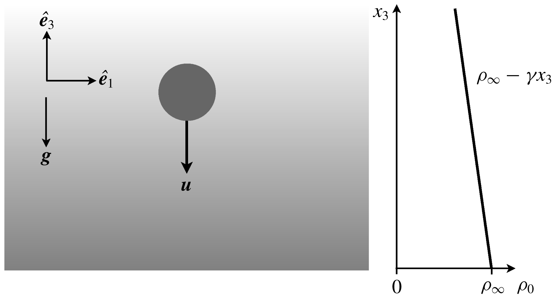
Settling of a sphere in a linearly stratified fluid with ambient density
 $\unicode[STIX]{x1D70C}_{0}=\unicode[STIX]{x1D70C}_{\infty }-\unicode[STIX]{x1D6FE}x_{3}$
where gravity
 $\boldsymbol{g}$
points in the negative
 $\hat{\boldsymbol{e}}_{3}$
-direction (we denote the basis in the laboratory frame by
 $\hat{\boldsymbol{e}}_{1}$
,
 $\hat{\boldsymbol{e}}_{2}$
and
 $\hat{\boldsymbol{e}}_{3}$
), and
 $x_{3}$
is the third component of the coordinate vector
 $\boldsymbol{x}$
in the laboratory frame. The particle settles with velocity
 $\boldsymbol{u}$
along gravity.

We consider a spherical particle of radius
 $a$
and of material density
 $\unicode[STIX]{x1D70C}_{p}$
settling with velocity
 $\boldsymbol{u}$
in a quiescent stratified fluid. The diffusivity of the stratifying agent (salt or temperature) is denoted by
 $\unicode[STIX]{x1D705}$
, and the kinematic viscosity of the fluid is denoted by
 $\unicode[STIX]{x1D708}$
. The ambient density of the fluid is assumed to vary linearly with height
 $x_{3}$
 $$\begin{eqnarray}\displaystyle \unicode[STIX]{x1D70C}_{0}=\unicode[STIX]{x1D70C}_{\infty }-\unicode[STIX]{x1D6FE}x_{3}, & & \displaystyle\end{eqnarray}$$
where
 $\unicode[STIX]{x1D6FE}$
is the density gradient, and
 $\unicode[STIX]{x1D70C}_{\infty }$
is a reference density. The problem is illustrated in figure 1. The settling particle causes disturbances in the fluid, in the local density
 $\unicode[STIX]{x1D70C}$
and in the pressure
 $p$
. To determine these disturbances one must solve the Navier–Stokes equation for the fluid velocity and the diffusion–advection equation for the density. Following Maxey & Riley (Reference Maxey and Riley1983) we express these equations in a frame of reference that translates with the particle position
 $\boldsymbol{x}_{p}(t)$
,
 $$\begin{eqnarray}\displaystyle & \displaystyle \unicode[STIX]{x1D70C}\left[\left.\frac{\unicode[STIX]{x2202}\boldsymbol{w}}{\unicode[STIX]{x2202}t}\right|_{\boldsymbol{r}}+(\boldsymbol{w}\boldsymbol{\cdot }\unicode[STIX]{x1D735})\boldsymbol{w}\right]=-\unicode[STIX]{x1D735}p+\unicode[STIX]{x1D707}\unicode[STIX]{x1D6AB}\boldsymbol{w}+\unicode[STIX]{x1D70C}\boldsymbol{g}-\unicode[STIX]{x1D70C}\frac{\unicode[STIX]{x2202}\boldsymbol{u}}{\unicode[STIX]{x2202}t}\quad \text{and}\quad \unicode[STIX]{x1D735}\boldsymbol{\cdot }\boldsymbol{w}=0, & \displaystyle\end{eqnarray}$$
 $$\begin{eqnarray}\displaystyle & \displaystyle \frac{\unicode[STIX]{x2202}\unicode[STIX]{x1D70C}}{\unicode[STIX]{x2202}t}+(\boldsymbol{w}\boldsymbol{\cdot }\unicode[STIX]{x1D735})\unicode[STIX]{x1D70C}=\unicode[STIX]{x1D705}\unicode[STIX]{x1D6AB}\unicode[STIX]{x1D70C}, & \displaystyle\end{eqnarray}$$
 $$\begin{eqnarray}\displaystyle & \displaystyle \boldsymbol{w}=\mathbf{0},\unicode[STIX]{x2202}_{r}\unicode[STIX]{x1D70C}=0\quad \text{at}~r=a\quad \text{and}\quad \boldsymbol{w}\rightarrow -\boldsymbol{u},\unicode[STIX]{x1D70C}\rightarrow \unicode[STIX]{x1D70C}_{0}\quad \text{as}~r\rightarrow \infty . & \displaystyle\end{eqnarray}$$
 $\boldsymbol{r}\equiv \boldsymbol{x}-\boldsymbol{x}_{p}$
, the spatial gradients
 $\unicode[STIX]{x1D735}$
are with respect to
 $\boldsymbol{r}$
and the fluid velocity is a function of
 $\boldsymbol{r}$
,
 $\boldsymbol{w}(\boldsymbol{r},t)$
. The boundary condition for
 $\unicode[STIX]{x1D70C}$
on the surface of the particle is derived from the surface condition
 $\unicode[STIX]{x1D735}\unicode[STIX]{x1D70C}\boldsymbol{\cdot }\boldsymbol{n}=0$
. This means that the particle surface is impermeable.
We define the disturbance velocity, density and pressure as:
 $$\begin{eqnarray}\displaystyle \boldsymbol{w}^{\prime }=\boldsymbol{w}+\boldsymbol{u},\quad \unicode[STIX]{x1D70C}^{\prime }=\unicode[STIX]{x1D70C}-\unicode[STIX]{x1D70C}_{0}\quad \text{and}\quad p^{\prime }=p-p_{0}. & & \displaystyle\end{eqnarray}$$
Here
 $p_{0}$
is the hydrostatic pressure,
 $\unicode[STIX]{x1D70C}_{0}$
is the ambient density at height
 $x_{3}$
and
 $-\boldsymbol{u}$
is the undisturbed fluid velocity in the frame translating with the particle.
We non-dimensionalise the problem in the usual fashion (Alias & Page Reference Alias and Page2017), using the particle radius
 $a$
for lengths, the typical time
 $\unicode[STIX]{x1D70F}$
of variation of the disturbance velocity induced by the boundary condition (2.2c
) for times, the terminal Stokes velocity in a homogeneous fluid
 $u_{t}=[2a^{2}/(9\unicode[STIX]{x1D708})](\unicode[STIX]{x1D70C}_{p}/\unicode[STIX]{x1D70C}_{\infty }-1)g$
for the fluid velocity,
 $\unicode[STIX]{x1D70C}_{\infty }\unicode[STIX]{x1D708}u_{t}/a$
for the pressure and
 $\unicode[STIX]{x1D6FE}a$
for the density. All equations below are written in these dimensionless variables.
We further assume that quadratic combinations of the density and pressure disturbances are negligible, and that
 $\unicode[STIX]{x1D6FE}x_{3}/\unicode[STIX]{x1D70C}_{\infty }\ll 1$
in the region of interest. This allows us to ignore density gradients except when multiplied by the gravitational acceleration (Gray & Giorgini Reference Gray and Giorgini1976). This ‘Boussinesq’ approximation was used in the DNS of the problem by Yick et al. (Reference Yick, Torres, Peacock and Stocker2009) and Zhang et al. (Reference Zhang, Mercier and Magnaudet2017) that we compare with § 5, see also Doostmohammadi et al. (Reference Doostmohammadi, Dabiri and Ardekani2014). Under these assumptions the non-dimensional equations for the disturbance velocity, density and pressure take the form
 $$\begin{eqnarray}\displaystyle & \displaystyle ReSl\frac{\unicode[STIX]{x2202}\boldsymbol{w}^{\prime }}{\unicode[STIX]{x2202}t}+Re[(\boldsymbol{w}^{\prime }\boldsymbol{\cdot }\unicode[STIX]{x1D735})\boldsymbol{w}^{\prime }-(\boldsymbol{u}\boldsymbol{\cdot }\unicode[STIX]{x1D735})\boldsymbol{w}^{\prime }]+Ri\,\unicode[STIX]{x1D70C}^{\prime }\hat{\boldsymbol{e}}_{3}=-\unicode[STIX]{x1D735}p^{\prime }+\unicode[STIX]{x1D6AB}\boldsymbol{w}^{\prime }\quad \text{and}\quad \unicode[STIX]{x1D735}\boldsymbol{\cdot }\boldsymbol{w}^{\prime }=0, & \displaystyle \nonumber\\ \displaystyle & & \displaystyle\end{eqnarray}$$
 $$\begin{eqnarray}\displaystyle & \displaystyle PeSl\frac{\unicode[STIX]{x2202}\unicode[STIX]{x1D70C}^{\prime }}{\unicode[STIX]{x2202}t}+Pe[(\boldsymbol{w}^{\prime }\boldsymbol{\cdot }\unicode[STIX]{x1D735})\unicode[STIX]{x1D70C}^{\prime }-(\boldsymbol{u}\boldsymbol{\cdot }\unicode[STIX]{x1D735})\unicode[STIX]{x1D70C}^{\prime }-\boldsymbol{w}^{\prime }\boldsymbol{\cdot }\hat{\boldsymbol{e}}_{3}]=\unicode[STIX]{x1D6AB}\unicode[STIX]{x1D70C}^{\prime }, & \displaystyle\end{eqnarray}$$
 $$\begin{eqnarray}\displaystyle & \displaystyle \boldsymbol{w}^{\prime }=\boldsymbol{u},\unicode[STIX]{x2202}_{r}\unicode[STIX]{x1D70C}^{\prime }=\cos \unicode[STIX]{x1D703}\quad \text{at}~r=1\quad \text{and}\quad \boldsymbol{w}^{\prime }\rightarrow \mathbf{0},\unicode[STIX]{x1D70C}^{\prime }\rightarrow 0\quad \text{as}~r\rightarrow \infty . & \displaystyle\end{eqnarray}$$
 $\unicode[STIX]{x1D703}$
is the angle between the outward unit normal
 $\boldsymbol{n}$
of the sphere and the vertical direction
 $\hat{\boldsymbol{e}}_{3}$
. The dimensionless parameters in (2.4a
) and (2.4b
) are the particle Reynolds number, the Péclet number, the Richardson number and the Strouhal number:
 $$\begin{eqnarray}\displaystyle Re=au_{t}/\unicode[STIX]{x1D708},\quad Pe=au_{t}/\unicode[STIX]{x1D705},\quad Ri=a^{3}N^{2}/(u_{t}\unicode[STIX]{x1D708}),\quad \text{and}\quad Sl=a/(u_{t}\unicode[STIX]{x1D70F}). & & \displaystyle\end{eqnarray}$$
Here
 $N$
is the Brunt–Väisälä frequency
 $$\begin{eqnarray}\displaystyle N=\sqrt{g\,\unicode[STIX]{x1D6FE}/\unicode[STIX]{x1D70C}_{\infty }}, & & \displaystyle\end{eqnarray}$$
the frequency at which a perturbation describing a vertically displaced parcel of fluid oscillates in a stably stratified environment (Mowbray & Rarity Reference Mowbray and Rarity1967). The Brunt–Väisälä frequency is an important physical parameter in problems involving stratified fluids, such as fountains (Bloomfield & Kerr Reference Bloomfield and Kerr1998; Mehaddi, Vauquelin & Candelier Reference Mehaddi, Vauquelin and Candelier2012), plumes (McDougall Reference McDougall1978; Woods Reference Woods2010; Mehaddi, Candelier & Vauquelin Reference Mehaddi, Candelier and Vauquelin2013) or gravity currents (Maxworthy et al. Reference Maxworthy, Leilich, Simpson and Meiburg2002), to name but a few.
We wrote (2.4) in a frame of reference translating with the particle. It is convenient to use such moving coordinates, because this simplifies the problem. For a sphere settling in a homogeneous flow, for example, the problem becomes steady. After a short transient, the buoyancy force balances the viscous drag so that the sphere reaches a steady terminal velocity. In a stratified fluid the situation is slightly more complicated. The problem appears to remain unsteady, because the settling sphere experiences a time-dependent buoyancy force since the ambient density
 $\unicode[STIX]{x1D70C}_{0}$
varies as a function of height
 $x_{3}$
. We now show under which circumstances this residual time dependence is negligible. The time scale
 $\unicode[STIX]{x1D70F}$
of variation of the disturbance velocity can be estimated as
 $\unicode[STIX]{x1D70F}^{-1}\sim \dot{u}_{t}/u_{t}$
where now
 $u_{t}\sim (2/9)(a^{2}g/\unicode[STIX]{x1D708})[\unicode[STIX]{x1D70C}_{p}/\unicode[STIX]{x1D70C}_{0}(t)-1]$
, and
 $\unicode[STIX]{x1D70C}_{0}(t)$
is the ambient density evaluated at the time-dependent particle position. We conclude that
 $$\begin{eqnarray}\displaystyle Sl\sim Ri\frac{\unicode[STIX]{x1D70C}_{p}}{\unicode[STIX]{x1D70C}_{\infty }}. & & \displaystyle\end{eqnarray}$$
In this paper we obtain the drag force on the sphere assuming that convective fluid inertia and density stratification matter, but that they are weak enough so that their effects can be treated in perturbation theory. We assume that
 $$\begin{eqnarray}\displaystyle 0<Re\ll 1\quad \text{and}\quad 0<Ri\ll 1. & & \displaystyle\end{eqnarray}$$
In this limit the unsteady terms in (2.4a ) and (2.4b ) are negligible, so that we can consider the steady problem.
3 Earlier results for
 $Re=0$

For
 $Re=0$
the drag on a sphere settling in a stratified fluid was studied theoretically by Zvirin & Chadwick (Reference Zvirin and Chadwick1975) and Candelier et al. (Reference Candelier, Mehaddi and Vauquelin2014). These authors made different assumptions concerning the relative importance of advection and diffusion in (2.4b
). Zvirin & Chadwick (Reference Zvirin and Chadwick1975) assumed that advection is more important than diffusion. When advection dominates, the density disturbance
 $\unicode[STIX]{x1D70C}^{\prime }$
scales as
 $z/r$
near the particle (Chadwick & Zvirin Reference Chadwick and Zvirin1974b
), in the ‘inner region’ of the problem. As a consequence, the buoyancy term in (2.4a
) balances the viscous Laplacian term at
 $$\begin{eqnarray}\displaystyle r\sim Ri^{-1/3}. & & \displaystyle\end{eqnarray}$$
At this distance inner and outer solutions of the disturbance problem must be matched. This implies that advection is more important than diffusion in (2.4b
) if
 $Pe>Ri^{1/3}$
. Second, at
 $r\sim Ri^{-1/3}$
the dominant convective inertial term in (2.4a
) is estimated as
 $Re(\boldsymbol{u}\boldsymbol{\cdot }\unicode[STIX]{x1D735})\boldsymbol{w}^{\prime (0)}\sim Re\,Ri^{2/3}$
, where
 $\boldsymbol{w}^{\prime (0)}\sim 1/r$
is the solution of the disturbance problem in the Stokes limit. So convective inertial terms are negligible if
 $Re\ll Ri^{1/3}$
. Under these conditions,
 $$\begin{eqnarray}\displaystyle Pe>Ri^{1/3}\quad \text{and}\quad Re\ll Ri^{1/3}, & & \displaystyle\end{eqnarray}$$
Zvirin & Chadwick (Reference Zvirin and Chadwick1975) derived the following expression for the drag force
 $$\begin{eqnarray}\displaystyle f_{3}=-6\unicode[STIX]{x03C0}u_{3}[1+B(Ri^{1/3}/Pe)Ri^{1/3}]. & & \displaystyle\end{eqnarray}$$
Here
 $B(\cdot )$
is a function given in integral form. In the limit of a non-diffusive fluid,
 $Pe\rightarrow \infty$
, the above expression simplifies to:
 $$\begin{eqnarray}\displaystyle f_{3}=-6\unicode[STIX]{x03C0}u_{3}(1+1.060\,Ri^{1/3}). & & \displaystyle\end{eqnarray}$$
Now consider the opposite limit, where the diffusive term in (2.4b
) dominates over the advective term. In this case Candelier et al. (Reference Candelier, Mehaddi and Vauquelin2014) showed that the spatial dependence of the disturbance density
 $\unicode[STIX]{x1D70C}^{\prime }$
is of the form
 $\unicode[STIX]{x1D70C}^{\prime }\sim Pe\,r$
in the inner region, so that the buoyancy term in (2.4a
) balances the Laplacian viscous term at
 $$\begin{eqnarray}\displaystyle r\sim \unicode[STIX]{x1D716}^{-1}\quad \text{with}~\unicode[STIX]{x1D716}=a/\ell _{s}. & & \displaystyle\end{eqnarray}$$
Here
 $\ell _{s}$
is the stratification length (Ardekani & Stocker Reference Ardekani and Stocker2010)
 $$\begin{eqnarray}\displaystyle \ell _{s}=(\unicode[STIX]{x1D708}\unicode[STIX]{x1D705}/N^{2})^{1/4}. & & \displaystyle\end{eqnarray}$$
It characterises the effect of stratification on the particle dynamics. Under the condition
 $$\begin{eqnarray}\displaystyle Pe\ll \unicode[STIX]{x1D716}\ll 1 & & \displaystyle\end{eqnarray}$$
Candelier et al. (Reference Candelier, Mehaddi and Vauquelin2014) found
 $$\begin{eqnarray}\displaystyle f_{3}=-6\unicode[STIX]{x03C0}u_{3}(1+0.6621\unicode[STIX]{x1D716}). & & \displaystyle\end{eqnarray}$$
Using
 $Ri=\unicode[STIX]{x1D716}^{4}/Pe$
, we see that the condition
 $Pe\ll \unicode[STIX]{x1D716}$
corresponds to
 $Pe\ll Ri^{1/3}$
. Comparing with the condition (3.2) it seems that the results (3.4) and (3.8) apply in the opposite limits of large and small Péclet numbers. Below we show, however, that the two approaches are in fact equivalent, although they seem to apply in distinct limits.
4 Method
We consider the same problem as Candelier et al. (Reference Candelier, Mehaddi and Vauquelin2014), but we do not neglect the fluid-inertia terms and the effect of advection of the fluid density by the disturbance flow. The relative importance of stratification and inertial effects is determined by the magnitude of the length scales
 $\ell _{s}$
and
 $\ell _{o}$
in relation to the particle size
 $a$
. Therefore we use
 $\unicode[STIX]{x1D716}=a/\ell _{s}$
(3.5) and
 $\ell _{s}/\ell _{o}$
as dimensionless parameters. The third parameter is the Prandtl number. In summary, we solve the steady limit of (2.4) to first order in the parameter
 $\unicode[STIX]{x1D716}$
using the method of asymptotic matching (Saffman Reference Saffman1965). Inner and outer solutions of the disturbance problem are matched at
 $r\sim \unicode[STIX]{x1D716}^{-1}$
in the limit
 $$\begin{eqnarray}\displaystyle \unicode[STIX]{x1D716}\ll 1,\quad \ell _{s}/\ell _{o}\ll \unicode[STIX]{x1D716}^{-1},\quad \text{and}~Pr~\text{arbitrary but fixed}. & & \displaystyle\end{eqnarray}$$
In this way we obtain an expression for drag force that is valid regardless of whether diffusion or advection dominates: our solution is valid in both limits considered by Zvirin & Chadwick (Reference Zvirin and Chadwick1975) and Candelier et al. (Reference Candelier, Mehaddi and Vauquelin2014), as well as uniformly in between.
Previous arguments, summarised in § 3, appeal to different behaviours of the density disturbance to show that the nonlinear convective terms
 $Re(\boldsymbol{w}^{\prime (0)}\boldsymbol{\cdot }\unicode[STIX]{x1D735})\boldsymbol{w}^{\prime (0)}$
and
 $Pe(\boldsymbol{w}^{\prime (0)}\boldsymbol{\cdot }\unicode[STIX]{x1D735})\unicode[STIX]{x1D70C}^{\prime }$
in (2.4) can be disregarded. A weakness of these arguments is that the limits of large and small
 $Pe$
are considered separately. This is not necessary in our formulation.
A general property of the method of asymptotic matching is that it is the magnitude of the different terms in the matching region that matters: all terms that are sub-leading in this region can be entirely neglected. As already mentioned in § 3, when
 $Re$
and
 $Ri$
are small, the disturbance velocity close to the particle is well approximated by the Stokes solution
 $\boldsymbol{w}^{\prime (0)}\sim 1/r$
. Assuming this dependence, we can estimate the magnitude of the nonlinear convective term
 $Re(\boldsymbol{w}^{\prime (0)}\boldsymbol{\cdot }\unicode[STIX]{x1D735})\boldsymbol{w}^{\prime (0)}$
in the matching region. Setting
 $r\sim \unicode[STIX]{x1D716}^{-1}$
we conclude that
 $Re(\boldsymbol{w}^{\prime (0)}\boldsymbol{\cdot }\unicode[STIX]{x1D735})\boldsymbol{w}^{\prime (0)}$
is small in this region compared with all other terms in (2.4a
), when
 $\unicode[STIX]{x1D716}$
is small. The orders of magnitude in (2.4b
) are more difficult to determine because the
 $\boldsymbol{r}$
-dependence of the density disturbance is not known unless
 $Pe$
is either small (Candelier et al.
Reference Candelier, Mehaddi and Vauquelin2014) or large (Zvirin & Chadwick Reference Zvirin and Chadwick1975). However, since
 $\boldsymbol{w}^{\prime (0)}\sim \unicode[STIX]{x1D716}$
in the matching region, we can conclude that the nonlinear term
 $Pe(\boldsymbol{w}^{\prime (0)}\boldsymbol{\cdot }\unicode[STIX]{x1D735})\unicode[STIX]{x1D70C}^{\prime }$
is negligible compared with
 $Pe(\boldsymbol{u}\boldsymbol{\cdot }\unicode[STIX]{x1D735})\unicode[STIX]{x1D70C}^{\prime }$
. As a result, equation (2.4) takes the form:
 $$\begin{eqnarray}\displaystyle & \displaystyle -\unicode[STIX]{x1D716}\,\frac{\ell _{s}}{\ell _{o}}(\boldsymbol{u}\boldsymbol{\cdot }\unicode[STIX]{x1D735})\boldsymbol{w}^{\prime }=-\unicode[STIX]{x1D735}p^{\prime }-\unicode[STIX]{x1D716}^{4}\tilde{\unicode[STIX]{x1D70C}}\hat{\boldsymbol{e}}_{3}+\unicode[STIX]{x1D6AB}\boldsymbol{w}^{\prime }\quad \text{and}\quad \unicode[STIX]{x1D735}\boldsymbol{\cdot }\boldsymbol{w}^{\prime }=0, & \displaystyle\end{eqnarray}$$
 $$\begin{eqnarray}\displaystyle & \displaystyle -\unicode[STIX]{x1D716}\,Pr\frac{\ell _{s}}{\ell _{o}}(\boldsymbol{u}\boldsymbol{\cdot }\unicode[STIX]{x1D735})\tilde{\unicode[STIX]{x1D70C}}-\boldsymbol{w}^{\prime }\boldsymbol{\cdot }\hat{\boldsymbol{e}}_{3}=\unicode[STIX]{x1D6AB}\tilde{\unicode[STIX]{x1D70C}}, & \displaystyle\end{eqnarray}$$
 $\unicode[STIX]{x1D70C}^{\prime }=Pe\,\tilde{\unicode[STIX]{x1D70C}}$
. The inner solution of (4.2) is obtained by a regular-perturbation expansion in
 $\unicode[STIX]{x1D716}$
. To obtain the outer solution one replaces the boundary condition on the particle surface by a singular source term (Saffman Reference Saffman1965). To lowest order in
 $\unicode[STIX]{x1D716}$
this term takes the form
 $6\unicode[STIX]{x03C0}\boldsymbol{u}\,\unicode[STIX]{x1D6FF}(\boldsymbol{r})$
, corresponding to the leading-order force exerted by the sphere on the fluid. Higher
 $\unicode[STIX]{x1D716}$
-orders in the source term contribute to the force at order
 $O(\unicode[STIX]{x1D716}^{2})$
, and need not be considered to order
 $\unicode[STIX]{x1D716}$
. Since the nonlinear convective terms are negligible, equation (4.2) is linear, so that the outer solution can be obtained by Fourier transform, for arbitrary values of
 $\unicode[STIX]{x1D716}$
. We define:
 $$\begin{eqnarray}\displaystyle \hat{f}(\boldsymbol{k})=\int \text{d}\boldsymbol{x}\,f(\boldsymbol{x})\text{e}^{-\text{i}\boldsymbol{k}\boldsymbol{\cdot }\boldsymbol{x}}\quad \text{and}\quad f(\boldsymbol{x})=\int \frac{\text{d}\boldsymbol{k}}{(2\unicode[STIX]{x03C0})^{3}}\hat{f}(\boldsymbol{k})\text{e}^{\text{i}\boldsymbol{k}\boldsymbol{\cdot }\boldsymbol{x}}. & & \displaystyle\end{eqnarray}$$
We expand the Fourier transform
 $\hat{\boldsymbol{w}}_{out}^{\prime }(\boldsymbol{k})$
of the outer solution in
 $\unicode[STIX]{x1D716}$
, in terms of generalised functions (Candelier, Mehaddi & Vauquelin Reference Candelier, Mehaddi and Vauquelin2013; Meibohm et al.
Reference Meibohm, Candelier, Rosen, Einarsson, Lundell and Mehlig2016):
 $$\begin{eqnarray}\displaystyle \hat{\boldsymbol{w}}_{out}^{\prime }=\hat{\boldsymbol{{\mathcal{T}}}}^{(0)}+\unicode[STIX]{x1D716}\hat{\boldsymbol{{\mathcal{T}}}}^{(1)}+\unicode[STIX]{x1D716}^{2}\hat{\boldsymbol{{\mathcal{T}}}}^{(2)}+\cdots \,. & & \displaystyle\end{eqnarray}$$
This method differs slightly from the standard approach (Saffman Reference Saffman1965) that formulates the outer problem in terms of strained coordinates
 $\overline{\boldsymbol{r}}=\unicode[STIX]{x1D716}\boldsymbol{r}$
. The advantage of the present approach is that it does not refer to any particular matching length scale – for instance the length scale at which the Laplacian is balanced by the buoyancy term in (4.2a
). The only requirement is that
 $\unicode[STIX]{x1D716}$
is small. For certain cases this approach is equivalent to using the reciprocal theorem to compute inertial corrections (Meibohm et al.
Reference Meibohm, Candelier, Rosen, Einarsson, Lundell and Mehlig2016).
The first two terms in the expansion (4.4) are obtained from
 $\hat{\boldsymbol{w}}_{out}^{\prime }$
as:
 $$\begin{eqnarray}\displaystyle \hat{\boldsymbol{{\mathcal{T}}}}^{(0)}=\lim _{\unicode[STIX]{x1D716}\rightarrow 0}\hat{\boldsymbol{w}}_{out}^{\prime }\quad \text{and}\quad \hat{\boldsymbol{{\mathcal{T}}}}^{(1)}=\lim _{\unicode[STIX]{x1D716}\rightarrow 0}\frac{1}{\unicode[STIX]{x1D716}}(\hat{\boldsymbol{w}}_{out}^{\prime }-\hat{\boldsymbol{{\mathcal{T}}}}^{(0)}). & & \displaystyle\end{eqnarray}$$
The first term,
 $\hat{\boldsymbol{{\mathcal{T}}}}^{(0)}(\boldsymbol{k})$
, is the Fourier transform of the solution of the outer problem at
 $\unicode[STIX]{x1D716}=0$
. The next term in the expansion takes the form
 $$\begin{eqnarray}\displaystyle \hat{\boldsymbol{{\mathcal{T}}}}^{(1)}(\boldsymbol{k})=\lim _{\unicode[STIX]{x1D716}\rightarrow 0}\frac{1}{\unicode[STIX]{x1D716}^{3}}\left[\hat{\boldsymbol{w}}_{out}^{\prime }\left(\frac{\boldsymbol{k}}{\unicode[STIX]{x1D716}}\right)-\hat{\boldsymbol{{\mathcal{T}}}}^{(0)}\left(\frac{\boldsymbol{k}}{\unicode[STIX]{x1D716}}\right)\right]. & & \displaystyle\end{eqnarray}$$
We evaluate this limit using the homogeneity properties of the functions
 $\hat{\boldsymbol{w}}_{out}^{\prime }(\boldsymbol{k})$
and
 $\hat{\boldsymbol{{\mathcal{T}}}}^{(0)}(\boldsymbol{k})$
(Candelier et al.
Reference Candelier, Mehaddi and Vauquelin2013; Meibohm et al.
Reference Meibohm, Candelier, Rosen, Einarsson, Lundell and Mehlig2016). This yields
 $$\begin{eqnarray}\displaystyle \hat{\boldsymbol{{\mathcal{T}}}}^{(1)}(\boldsymbol{k})=\unicode[STIX]{x1D6FF}(\boldsymbol{k})\int \text{d}\boldsymbol{k}^{\prime }[\hat{\boldsymbol{w}}_{out}^{\prime }|_{\unicode[STIX]{x1D716}=1}(\boldsymbol{k}^{\prime })-\hat{\boldsymbol{{\mathcal{T}}}}^{(0)}(\boldsymbol{k}^{\prime })]. & & \displaystyle\end{eqnarray}$$
Here
 $\unicode[STIX]{x1D6FF}$
is the three-dimensional Dirac delta function. The functions
 $\hat{\boldsymbol{{\mathcal{T}}}}^{(0)}(\boldsymbol{k})$
and
 $\hat{\boldsymbol{{\mathcal{T}}}}^{(1)}(\boldsymbol{k})$
are readily transformed back from
 $\boldsymbol{k}$
to obtain the outer solution in configuration space. In particular,
 $\boldsymbol{{\mathcal{T}}}^{(1)}(\boldsymbol{r})$
is found to be
 $\boldsymbol{r}$
-independent. Since
 $\boldsymbol{{\mathcal{T}}}^{(1)}(\boldsymbol{r})$
is constant, the problem to order
 $\unicode[STIX]{x1D716}$
is equivalent to determining the force on a particle kept fixed in a uniform flow (Saffman Reference Saffman1965; Meibohm et al.
Reference Meibohm, Candelier, Rosen, Einarsson, Lundell and Mehlig2016). It follows that the drag force is given by
 $$\begin{eqnarray}\displaystyle \boldsymbol{f}=-6\unicode[STIX]{x03C0}\left\{\boldsymbol{u}+\frac{\unicode[STIX]{x1D716}}{8\unicode[STIX]{x03C0}^{3}}\int \text{d}\boldsymbol{k}^{\prime }[\hat{\boldsymbol{w}}_{out}^{\prime }(\boldsymbol{k}^{\prime })|_{\unicode[STIX]{x1D716}=1}-\hat{\boldsymbol{{\mathcal{T}}}}^{(0)}(\boldsymbol{k}^{\prime })]\right\}. & & \displaystyle\end{eqnarray}$$
We note that the force is determined entirely by the solution of the outer problem, as first shown by Saffman (Reference Saffman1965) for the lift force on a small sphere in a shear flow.
5 Results
For
 $\unicode[STIX]{x1D716}=1$
the Fourier transforms
 $\hat{\boldsymbol{w}}_{out}^{\prime }$
and
 $\hat{\tilde{\unicode[STIX]{x1D70C}}}_{out}$
of the outer solution read:
 $$\begin{eqnarray}\displaystyle \left(\begin{array}{@{}c@{}}\hat{\boldsymbol{w}}_{out}^{\prime }\\ \hat{\tilde{\unicode[STIX]{x1D70C}}}_{out}\end{array}\right)=-6\unicode[STIX]{x03C0}\,k^{2}\left[\frac{\ell _{s}}{\ell _{o}}(\text{i}\boldsymbol{k}\boldsymbol{\cdot }\boldsymbol{u})\unicode[STIX]{x1D644}+\unicode[STIX]{x1D63C}\right]^{-1}\boldsymbol{\cdot }\unicode[STIX]{x1D642}\boldsymbol{\cdot }\left(\begin{array}{@{}c@{}}\boldsymbol{u}\\ 0\end{array}\right). & & \displaystyle\end{eqnarray}$$
Here
 $\unicode[STIX]{x1D644}$
is the
 $4\times 4$
unit tensor, and
 $$\begin{eqnarray}\displaystyle \unicode[STIX]{x1D63C}=\left(\begin{array}{@{}cccc@{}}-k^{2} & 0 & 0 & \displaystyle -\frac{k_{1}k_{3}}{k^{2}}\\ 0 & -k^{2} & 0 & \displaystyle -\frac{k_{2}k_{3}}{k^{2}}\\ 0 & 0 & -k^{2} & \displaystyle -\frac{(k^{2}-k_{3}^{2})}{k^{2}}\\ 0 & 0 & \displaystyle \frac{1}{Pr} & \displaystyle -\frac{k^{2}}{Pr}\end{array}\right),\quad \unicode[STIX]{x1D642}=\left(\begin{array}{@{}cccc@{}}\displaystyle \frac{k^{2}-k_{1}^{2}}{k^{4}} & \displaystyle -\frac{k_{1}k_{2}}{k^{4}} & \displaystyle -\frac{k_{1}k_{3}}{k^{4}} & 0\\ \displaystyle -\frac{k_{2}k_{1}}{k^{4}} & \displaystyle \frac{k^{2}-k_{2}^{2}}{k^{4}} & \displaystyle -\frac{k_{2}k_{3}}{k^{4}} & 0\\ \displaystyle -\frac{k_{3}k_{1}}{k^{4}} & \displaystyle -\frac{k_{3}k_{2}}{k^{4}} & \displaystyle \frac{k^{2}-k_{3}^{2}}{k^{4}} & 0\\ 0 & 0 & 0 & 0\end{array}\right). & & \displaystyle \nonumber\\ \displaystyle & & \displaystyle\end{eqnarray}$$
We set
 $\boldsymbol{u}=u_{3}\hat{\boldsymbol{e}}_{3}$
in (4.8) to find the drag force on the settling sphere:
 $$\begin{eqnarray}\displaystyle & \displaystyle f_{3}=-6\unicode[STIX]{x03C0}u_{3}(1+\unicode[STIX]{x1D716}\,M_{33}), & \displaystyle\end{eqnarray}$$
 $$\begin{eqnarray}\displaystyle & \displaystyle M_{33}=\frac{3}{2\unicode[STIX]{x03C0}}\int _{0}^{\infty }\text{d}k\int _{0}^{\unicode[STIX]{x03C0}}\text{d}\unicode[STIX]{x1D703}\,\frac{\sin (\unicode[STIX]{x1D703})^{3}\left\{1-\left[Pr\left(\displaystyle \frac{\ell _{s}}{\ell _{o}}\right)^{2}k^{2}+1\right]\cos (\unicode[STIX]{x1D703})^{2}-\text{i}\cos (\unicode[STIX]{x1D703})\displaystyle \frac{\ell _{s}}{\ell _{o}}k^{3}\right\}}{\left[Pr\left(\displaystyle \frac{\ell _{s}}{\ell _{o}}\right)^{2}k^{2}+1\right]\cos (\unicode[STIX]{x1D703})^{2}+\text{i}\displaystyle \frac{\ell _{s}}{\ell _{o}}k^{3}(Pr+1)\cos (\unicode[STIX]{x1D703})-k^{4}-1}. & \displaystyle \nonumber\\ \displaystyle & & \displaystyle\end{eqnarray}$$


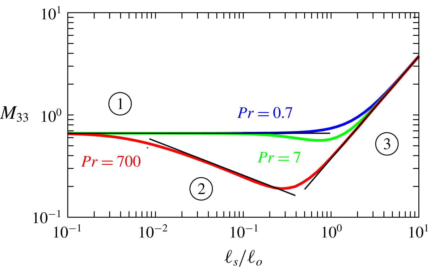
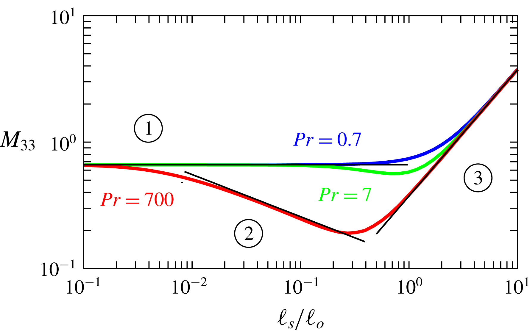
Figure 2 shows how
 $M_{33}$
depends on the ratio
 $\ell _{s}/\ell _{o}$
for different values of
 $Pr$
, namely, 0.7 (temperature-stratified gas), 7 (temperature-stratified water at
 $20\,^{\circ }\text{C}$
) and 700 (salt-stratified water). When the ratio
 $\ell _{s}/\ell _{o}$
is very small, the curves collapse onto a horizontal line, equation (3.8). In this limit diffusion dominates. When
 $\ell _{s}/\ell _{o}$
reaches
 $Pr^{-1}$
, a second regime emerges: diffusion and advection in (2.4b
) become of the same order, resulting in a change in the behaviour of the density disturbance. As a result,
 $M_{33}$
in figure 2 turns downwards as
 $\ell _{s}/\ell _{o}$
increases (this does not mean that the drag
 $-6\unicode[STIX]{x03C0}u_{3}(1+\unicode[STIX]{x1D716}M_{33})$
increases at fixed particle radius
 $a$
and Reynolds number
 $Re$
, because
 $\unicode[STIX]{x1D716}=a/\ell _{s}$
). A further transition occurs at
 $\ell _{s}/\ell _{o}\sim 1/Pr^{1/4}$
, caused by the formation of an Oseen wake behind the particle (Lovalenti & Brady Reference Lovalenti and Brady1993). When
 $\ell _{s}/\ell _{o}\gg 1/Pr^{1/4}$
the curves approach
 $M_{33}\approx (3/8)(\ell _{s}/\ell _{o})$
, the Oseen correction (Oseen Reference Oseen1910; Proudman & Pearson Reference Proudman and Pearson1957; Lovalenti & Brady Reference Lovalenti and Brady1993). In this regime stratification and diffusion do not matter, the settling particle experiences the fluid as if it were homogeneous. For small
 $Pr$
, only the first and third regimes are realised.
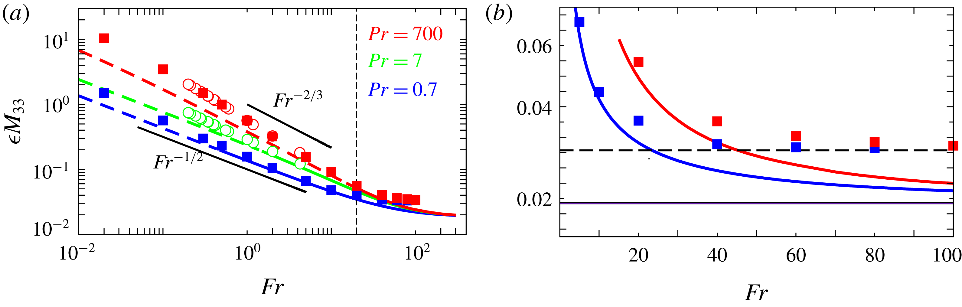
(a) Comparison between (5.3b
) and DNS results for
 $Re=0.05$
by Yick et al. (Reference Yick, Torres, Peacock and Stocker2009) for
 $Pr=7$
(○, green),
 $Pr=700$
(○, red) and by Zhang et al. (Reference Zhang, Mercier and Magnaudet2017) for
 $Pr=0.7$
(▪, blue) and
 $Pr=700$
(▪, red). Coloured solid lines show (5.3b
) for
 $\unicode[STIX]{x1D716}<\unicode[STIX]{x1D716}_{0}$
, dashed lines for
 $\unicode[STIX]{x1D716}>\unicode[STIX]{x1D716}_{0}$
, for a small value of
 $\unicode[STIX]{x1D716}_{0}$
. We take
 $\unicode[STIX]{x1D716}_{0}=0.3$
. Also shown are power laws in
 $Fr$
, black solid lines. The vertical dashed line corresponds to
 $Fr=1/Re$
. (b) Same data as in (a) but now with linear axes to emphasise the deviations between theory and DNS at large
 $Fr$
. The black dashed line shows the drag for the finite homogeneous system obtained by Zhang et al. (Reference Zhang, Mercier and Magnaudet2017). The solid black line shows the theoretical value for the homogeneous infinite system.

Equation (5.3b
) is uniformly valid in the limit (4.1), regardless of the value of
 $(\ell _{s}/\ell _{o})Pr=(Ri^{1/3}/Pe)^{-3/4}$
. It is not necessary to assume that
 $Pe\ll Ri^{1/3}$
, the expression holds also when
 $Pe\gg Ri^{1/3}$
. In particular, we can see that (5.3b
) reduces to (3.3) when convective inertia is negligible, by taking the limit
 $\ell _{s}/\ell _{o}\rightarrow 0$
at fixed
 $(\ell _{s}/\ell _{o})Pr$
:
 $$\begin{eqnarray}\displaystyle \lim _{\ell _{s}/\ell _{o}\rightarrow 0}M_{33}=\frac{3\,Ri^{1/3}}{\unicode[STIX]{x03C0}\unicode[STIX]{x1D716}}\int _{0}^{\infty }\text{d}k\int _{0}^{\unicode[STIX]{x03C0}/2}\text{d}\unicode[STIX]{x1D703}\frac{\sin (\unicode[STIX]{x1D703})^{5}(\sin (\unicode[STIX]{x1D703})^{2}+(Ri^{1/3}/Pe)k^{4})}{(\sin (\unicode[STIX]{x1D703})^{2}+(Ri^{1/3}/Pe)k^{4})^{2}+\cos (\unicode[STIX]{x1D703})^{2}k^{6}}. & & \displaystyle\end{eqnarray}$$
This is precisely the function
 $B(\cdot )$
in (3.3) (equation (29) in Zvirin & Chadwick (Reference Zvirin and Chadwick1975)), computed assuming that convective inertia is negligible, and that
 $Pe>Ri^{1/3}$
. Since our solution is uniformly valid, we can conclude that (3.3) must be valid also for
 $Pe\ll Ri^{1/3}$
, well outside the region of validity stated by Zvirin & Chadwick (Reference Zvirin and Chadwick1975). Closer inspection of their calculation shows that it corresponds to asymptotic matching at
 $r\sim Ri^{-1/3}$
in the limit
 $Ri\rightarrow 0$
keeping
 $Ri^{1/3}/Pe$
constant. The two different matching scales
 $r\sim Ri^{-1/3}$
and
 $r\sim \unicode[STIX]{x1D716}^{-1}$
are equivalent in the limits stated, because the ratio of matching scales
 $Ri^{1/3}/\unicode[STIX]{x1D716}=(Ri^{1/3}/Pe)(Pe/\unicode[STIX]{x1D716})=(Ri^{1/3}/Pe)[(\ell _{s}/\ell _{o})Pr]$
remains constant. In summary, equation (5.3b
) is a uniform approximation comprising three distinct regimes
 $$\begin{eqnarray}\displaystyle f_{3}\sim -6\unicode[STIX]{x03C0}u_{3}\left\{\begin{array}{@{}lll@{}}1+0.6621\unicode[STIX]{x1D716} & \text{for}~\ell _{s}/\ell _{o}\ll Pr^{-1} & \text{regime}~\unicode[STIX]{x2460}~\text{(diffusion),}\\ 1+1.060\,Ri^{1/3} & \text{for}~Pr^{-1}\ll \ell _{s}/\ell _{o}\ll Pr^{-1/4} & \text{regime}~\unicode[STIX]{x2461}~\text{(advection),}\\ 1+{\textstyle \frac{3}{8}}\,Re & \text{for}~\ell _{s}/\ell _{o}\gg Pr^{-1/4} & \text{regime}~\unicode[STIX]{x2462}~\text{(fluid inertia)}.\end{array}\right. & & \displaystyle \nonumber\\ \displaystyle & & \displaystyle\end{eqnarray}$$
The different regimes are shown in figure 2. In the limit of small
 $Pr$
, the advective regime disappears, as mentioned above.
We now compare the full result, equation (5.3b
), with DNS by Yick et al. (Reference Yick, Torres, Peacock and Stocker2009) and Zhang et al. (Reference Zhang, Mercier and Magnaudet2017), at their smallest
 $Re$
. These authors use slightly different dimensionless parameters, namely
 $Re$
,
 $Pr$
and the Froude number
 $Fr$
 $$\begin{eqnarray}\displaystyle Fr=u_{t}/(a\,N). & & \displaystyle\end{eqnarray}$$
In terms of
 $Fr$
, the dimensionless parameters
 $\unicode[STIX]{x1D716}$
,
 $\ell _{s}/\ell _{o}$
, and
 $Ri$
are given by:
 $$\begin{eqnarray}\displaystyle \unicode[STIX]{x1D716}=(Re/Fr)^{1/2}Pr^{1/4},\quad \ell _{s}/\ell _{o}=(Re\,Fr)^{1/2}/Pr^{1/4},\quad \text{and}\quad Ri^{1/3}=Re^{1/3}/Fr^{2/3}. & & \displaystyle\end{eqnarray}$$
Yick et al. (Reference Yick, Torres, Peacock and Stocker2009) and Zhang et al. (Reference Zhang, Mercier and Magnaudet2017) computed the drag coefficient
 $C_{D}^{S}$
of the stratified system. In figure 3(a) we plot their result for
 $C_{D}^{S}/C_{D}^{Stokes}-1$
versus
 $Fr$
, and compare it with our result for
 $\unicode[STIX]{x1D716}M_{33}$
. Here
 $C_{D}^{Stokes}=12/Re$
is the Stokes drag coefficient for an unbounded system. Since (5.3b
) was obtained for small
 $\unicode[STIX]{x1D716}$
, we plot it as a solid line when
 $\unicode[STIX]{x1D716}<0.3$
, and dashed for
 $\unicode[STIX]{x1D716}>0.3$
. For
 $1<Fr<10$
the data for
 $Pr=0.7$
are in the diffusive regime, where the correction to the drag scales as
 $Fr^{-1/2}$
. For
 $Pr=700$
, the data approach the advection regime where the theory predicts that the drag correction scales as
 $Ri^{1/3}\propto Fr^{-2/3}$
.
Figure 3(a) shows that the DNS yield a larger drag coefficient than our theory when
 $Fr$
is small. The likely reason is that the nonlinear convective terms matter in this regime, because
 $\unicode[STIX]{x1D716}$
is not small enough (dashed lines in figure 3(a) indicate that
 $\unicode[STIX]{x1D716}>0.3$
, as mentioned above). For
 $Pr=700$
, for example,
 $\unicode[STIX]{x1D716}$
becomes larger than 0.3 when
 $Fr$
falls below 14.7 at
 $Re=0.05$
.
When do convective fluid-inertia effects dominate? The condition
 $\ell _{s}/\ell _{o}=1/Pr^{1/4}$
corresponds to
 $Fr=1/Re$
, independent of Prandtl number. For
 $Re=0.05$
– the smallest value used in the DNS – this cross-over occurs at
 $Fr=20$
, indicated by the vertical black dashed line in figure 3(a). Equation (5.3b
) allows us to determine the relative importance of convective fluid inertia at this value of
 $Fr$
. For
 $Pr=0.7$
the correction is substantial, 13.5 %. For larger Péclet numbers the correction is smaller, 1.4 % at
 $Pr=7$
, and 2 % at
 $Pr=700$
. That the correction is largest for small
 $Pr$
can be inferred from figure 3(a).
We observe deviations between DNS and theory not only at small values of
 $Fr$
, discussed above, but also at large values of
 $Fr$
(figure 3
b). These deviations at large
 $Fr$
may be due to finite-size effects. In this limit, the homogeneous Oseen correction dominates, and it is known to be quite sensitive to the size of the simulation domain. Yick et al. (Reference Yick, Torres, Peacock and Stocker2009) chose an elliptical simulation domain, with a smallest size
 $L$
that gives
 $L/(2a)=40$
. The domain used by Zhang et al. (Reference Zhang, Mercier and Magnaudet2017) was spherical and larger (
 $\text{diameter}/(2a)=80$
), but even in that case a theory for cylindrical domains (Happel & Brenner Reference Happel and Brenner1983) indicates that the drag correction is expected to be larger than the Oseen expression
 $(3/8)Re$
. This is consistent with figure 3(b). We also see that the asymptotic value for the homogeneous fluid is reached more quickly in the finite system. Finite-size effects matter less for smaller
 $Fr$
, because the wake is smaller, of order
 $\ell _{s}$
.
6 Conclusions
We calculated how convective fluid inertia modifies the drag on a sphere slowly settling in a density-stratified fluid, at small Richardson and Reynolds numbers. Plotting the results as a function of the dimensionless parameter
 $\ell _{s}/\ell _{o}$
reveals three distinct regimes, equation (5.5). In the first regime, the drag is determined by diffusion of the disturbance density. In the second regime, advection of the disturbance density determines the drag. In the third regime, convection of the disturbance density by fluid-inertia terms dominates. Our main result, equation (5.3b
), is uniformly valid, independently of whether the density dynamics is diffusive or advective. This allowed us to show that a result by Zvirin & Chadwick (Reference Zvirin and Chadwick1975) is more generally valid than the authors stated.
We compared with recent DNS at small
 $Re$
and found that convective fluid-inertia effects matter for the larger Froude numbers simulated. Since finite-size effects appear to be important at large
 $Fr$
and small
 $Re$
, it would be of interest to take these corrections into account in the theory.
The results derived in this paper were obtained in the steady limit. But when a particle is released from above the water surface and plunges into the fluid with a given velocity, then unsteady effects must matter, at least initially. DNS of the problem (Doostmohammadi et al.
Reference Doostmohammadi, Dabiri and Ardekani2014) at
 $Re$
of order unity reveal unsteady effects that depend on the dimensionless numbers of the problem in intricate ways.
A further motivation for considering unsteady effects concerns the unsteady swimming of micro-organisms in stratified fluids (Bergström & Strömberg Reference Bergström and Strömberg1997; Jephson & Carlsson Reference Jephson and Carlsson2009; Doostmohammadi, Stocker & Ardekani Reference Doostmohammadi, Stocker and Ardekani2012). In oceans or in lakes the surface layers are known to shelter substantial biological activity. For very small organisms (much smaller than 1 mm in size in typical ocean conditions) the dynamics of swimming microorganisms is well understood. Buoyancy (Franks & Jaffe Reference Franks and Jaffe2008), density or drag asymmetries of the body (Roberts Reference Roberts1970; Kessler Reference Kessler1985; Jonsson Reference Jonsson1989), and turbulence (Durham et al. Reference Durham, Climent, Barry, de Lillo, Boffetta, Cencini and Stocker2013; Gustavsson et al. Reference Gustavsson, Berglund, Jonsson and Mehlig2016) determine the spatial distribution of these organisms, their encounter rates and thus their population ecology (Guasto et al. Reference Guasto, Rusconi and Stocker2012). For larger organisms less is known. The problem becomes considerably more difficult because inertial effects begin to matter (Wang & Ardekani Reference Wang and Ardekani2012b ,Reference Wang and Ardekani a ). The method described here allows us to take inertial effects into account in perturbation theory. Finally, an important problem is how fluid shears affect the dynamics of motile microorganisms. The approach described by Candelier, Mehlig & Magnaudet (Reference Candelier, Mehlig and Magnaudet2018) makes it possible to address this question.
Acknowledgements
We thank J. Magnaudet and J. Zhang for providing some of the numerical data discussed in Zhang et al. (Reference Zhang, Mercier and Magnaudet2017). B.M. was supported by Vetenskapsrådet (grant number 2017-03865), Formas (grant number 2014-585) and by the grant ‘Bottlenecks for particle growth in turbulent aerosols’ from the Knut and Alice Wallenberg Foundation, Dnr. KAW 2014.0048.