1 Introduction
The flow of fluids around and inside solid bodies is ubiquitous in industry and transport, with near-wall turbulence being recognized as one of the key fundamental issues for the modelling of most of these flows of practical interest and representing the Achilles heel of turbulence models. This is partly due to the lack of reliable measurements very close to the wall at sufficiently high Reynolds numbers to be relevant for practical applications (Smits, McKeon & Marusic Reference Smits, McKeon and Marusic2011). Even the smallest hot-wire probes have difficulties very close to the wall at high Reynolds numbers (Hultmark et al. Reference Hultmark, Vallikivi, Bailey and Smits2013). An improved characterization and understanding of the very-near-wall turbulence is essential to build more reliable models and eventually provide the necessary knowledge to yield viable methods that will reduce the drag, one of the key issues in the present context of energy savings.
The key problem in currently available measurements is that even in large facilities, the high Reynolds number leads to very small scales near the wall, which are impossible to resolve with the standard laboratory measurement tools that are currently employed around the world.
Previous experimental measurements of high-Reynolds-number pipe flows are mainly available from Princeton’s SuperPipe facility (Hultmark et al.
Reference Hultmark, Vallikivi, Bailey and Smits2012, Reference Hultmark, Vallikivi, Bailey and Smits2013). Due to the small viscous length scales in this facility (
 $l^{\ast }=\unicode[STIX]{x1D708}/u_{\unicode[STIX]{x1D70F}}<1~\unicode[STIX]{x03BC}\text{m}$
at
 $Re_{\unicode[STIX]{x1D70F}}=u_{\unicode[STIX]{x1D70F}}R/\unicode[STIX]{x1D708}=70\,000$
, with
 $R$
the pipe radius,
 $\unicode[STIX]{x1D708}$
the kinematic viscosity and
 $u_{\unicode[STIX]{x1D70F}}$
the shear velocity), measurements were performed with specialized micro-fabricated hot-wire probes (NSTAP). Yet even these probes were not able to adequately resolve the velocity profile in the viscous layer immediately adjacent to the wall (
 $y^{+}<15$
) as they had a length in viscous units,
 $l^{+}=60$
, that was well beyond the maximum of
 $l^{+}=20$
recommended by Ligrani & Bradshaw (Reference Ligrani and Bradshaw1987) and Hutchins et al. (Reference Hutchins, Nickels, Marusic and Chong2009) to keep the error to less than 10 % in the streamwise Reynolds stress. Information on the evolution of the inner turbulence peak, considered to be the primary source of turbulence production (Pullin, Inoue & Saito Reference Pullin, Inoue and Saito2013), is thus very limited and inconclusive.
This type of information is available from direct numerical simulations (DNS) of turbulence pipe flow which were performed by Ahn et al. (Reference Ahn, Lee, Lee, Kang and Sung2015) for
 $Re_{\unicode[STIX]{x1D70F}}\approx 3000$
and for channel flow up to
 $Re_{\unicode[STIX]{x1D70F}}\approx 5200$
by Lee & Moser (Reference Lee and Moser2015). The Reynolds numbers of these simulations are still an order of magnitude smaller than those of currently available high-
 $Re_{\unicode[STIX]{x1D70F}}$
pipe flow experiments. At these lower Reynolds numbers, the so-called outer peak starts to appear but does not yet exhibit a distinct peak or plateau (it appears around
 $Re_{\unicode[STIX]{x1D70F}}\approx 20\,000$
).
Aside from the data available from the Princeton SuperPipe, wall-normal profiles of the streamwise Reynolds stress have been measured by Schultz & Flack (Reference Schultz and Flack2013) for channel flows up to
 $Re_{\unicode[STIX]{x1D70F}}=6000$
, indicating that the inner peak increases with increasing Reynolds number, a trend that thus far could not be confirmed for pipe flows at similar or higher Reynolds numbers. However, it is also worth noting that in the study of Schultz & Flack (Reference Schultz and Flack2013), which used laser Doppler velocimetry (LDV), the viscous length scale of
 $l^{\ast }=2~\unicode[STIX]{x03BC}\text{m}$
at
 $Re_{\unicode[STIX]{x1D70F}}=6000$
only allowed for measurements down to
 $y^{+}\approx 20$
.
In this paper, we report on two-component–two-dimensional (2C–2D) near-wall velocity measurements of turbulent pipe flow at shear Reynolds numbers in the range
 $Re_{\unicode[STIX]{x1D70F}}=5000{-}40\,000$
acquired in the Long Pipe facility in CICLOPE (Center for International Cooperation in Long Pipe Experiments) of the University of Bologna, located in Predappio, Italy (Talamelli et al.
Reference Talamelli, Persiani, Fransson, Alfredsson, Johansson, Nagib, Redi, Sreenivasan and Monkewitz2009; Örlü et al.
Reference Örlü, Fiorini, Segalini, Bellani, Talamelli and Alfredsson2017). As a consequence of the installation site and the characteristic dimensions of the facility, the Long Pipe offers viscous length scales that can be resolved using conventional imaging hardware. Despite the fact that spatial resolution effects prevent accurate measurements of the streamwise variance at the inner peak for Reynolds numbers above 28 000, the resolution is sufficient to determine the increasing trend of the inner peak. However, more generally, the new 2C–2D near-wall measurements reported here represent the highest-spatial-resolution
 $(u,v)$
velocity measurements up to
 $Re_{\unicode[STIX]{x1D70F}}=40\,000$
compared with previous published results (Hutchins et al.
Reference Hutchins, Nickels, Marusic and Chong2009; Hultmark et al.
Reference Hultmark, Vallikivi, Bailey and Smits2013; Örlü et al.
Reference Örlü, Fiorini, Segalini, Bellani, Talamelli and Alfredsson2017) – noting that Hutchins et al. (Reference Hutchins, Nickels, Marusic and Chong2009) and Hultmark et al. (Reference Hultmark, Vallikivi, Bailey and Smits2013) only measured the streamwise
 $u$
-velocity component, while Örlü et al. (Reference Örlü, Fiorini, Segalini, Bellani, Talamelli and Alfredsson2017) measured the
 $(u,v)$
-velocity components at selected points using their probe.
2 Experimental technique
2.1 The CICLoPE facility
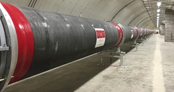
The Long Pipe (LP) is a unique facility for the study of high-Reynolds-number fully developed turbulent pipe flow. With a diameter of 0.9 m and a length of 111.5 m, the LP operates with air at ambient pressure in a closed loop with a 200 kW axial fan in the return duct (figure 1). A cooling unit ensures temperature stability within
 $\pm 0.1\,^{\circ }\text{C}$
. The LP is made of 5 m long carbon-fibre sections with a surface roughness of
 $k_{rms}\approx 0.2~\unicode[STIX]{x03BC}\text{m}$
. At centreline velocities between 5 and
 $40~\text{m}~\text{s}^{-1}$
, the turbulent pipe flow has viscous length scales ranging from
 $l^{\ast }=85~\unicode[STIX]{x03BC}\text{m}$
at
 $Re_{\unicode[STIX]{x1D70F}}=5000$
down to
 $l^{\ast }=11~\unicode[STIX]{x03BC}\text{m}$
at
 $Re_{\unicode[STIX]{x1D70F}}=40\,000$
. The wall friction,
 $\unicode[STIX]{x1D70F}_{w}$
, is determined by linearly fitting six static pressure measurements in the last portion of the LP (
 $88<L/D<122$
), where the flow is assumed to be fully developed. The static pressure is measured through 1 mm wall taps placed with a 5 m spacing along the pipe. The estimated uncertainty in
 $\unicode[STIX]{x1D70F}_{w}$
is below
 $\pm 0.25\,\%$
, as reported in Fiorini (Reference Fiorini2017).
Photograph of the 111.5 m long CICLoPE facility, with the measurement location seen at the far end.

2.2 The particle image velocimetry technique
The reported length scales of
 $l^{\ast }=11{-}85~\unicode[STIX]{x03BC}\text{m}$
can be resolved with a high-speed particle image velocimetry (PIV) camera at image magnification near unity. The employed PIV measurement approach closely follows the procedures and methods laid out by Willert (Reference Willert2015) to capture the wall-normal velocity profile and higher-order statistics. The near-wall measurement approach has been successfully used in a variety of previous applications; however, with viewing arrangements involving straight walls (Soria et al.
Reference Soria, Willert, Amili, Klinner, Atkinson, Stanislas, Schröder, Geisler, Agocs and Röse2016; Cuvier et al.
Reference Cuvier, Srinath, Stanislas, Foucaut, Laval, Kähler, Hain, Scharnowski, Schröder and Geisler2017). Application of the technique in the curved convex contour of the pipe required the design of a new imaging approach. In order to obtain a reasonably orthogonal view of the near-wall region, a specific circular insert was designed to accommodate a thin
 $45^{\circ }$
high-aspect mirror that was placed approximately 50 mm from the area of interest (figure 2
b). While the mirror did protrude into the flow, it had a low cross-section (1 mm thickness), considered to have only a minor influence in the imaged domain.
The imaging set-up was designed for a magnification of unity (
 $m=1.0$
) using a macroscopic lens of 200 mm focal length (Nikon Micro-Nikkor
 $200/4$
) at a maximum aperture of
 $f^{\#}=5.6$
. During the measurements, the aperture could be reduced to
 $f^{\#}$
in the range 8–11 due to the high energy levels provided by a pulsed high-speed laser (Quantronix Darwin Duo), resulting in an estimated depth of field ranging from
 $660~\unicode[STIX]{x03BC}\text{m}$
at
 $f^{\#}=8$
to 1.26 mm at
 $f^{\#}=11$
. The approximately
 $300\pm 100~\unicode[STIX]{x03BC}\text{m}$
thin laser light sheet was introduced radially into the pipe (figure 2
a,b). Thus, the size of the measurement volume in the direction normal to the streamwise-wall-normal plane was given by the thickness of the laser sheet. The PIV image acquisition was undertaken using a high-speed camera with a 4 megapixel CMOS sensor (PCO AG, DIMAX-S4), which had a pixel pitch of
 $11~\unicode[STIX]{x03BC}\text{m}$
. Using macroscopic imaging at unity, the smallest viscous scales at the facility design point of
 $Re_{\unicode[STIX]{x1D70F}}=40\,000$
matched the pixel size. The field of view of the camera was reduced to 178 or 200 pixel width and varied in height between 1008 and 2016 pixels. This reduction allowed an increase in the number of acquired image pairs (i.e. velocity fields) to more than 70 000 during a single run.
Seeding of
 $1~\unicode[STIX]{x03BC}\text{m}$
droplets was provided globally for the PIV experiments via a smoke generator using a water–glycol mixture, which was injected into the flow downstream of the test section, allowing it to mix thoroughly before reaching the measurement area after running the full length of the return duct and pipe.
(a) Photograph of the PIV set-up on the CICLoPE facility and (b) schematic of the insert for near-wall PIV measurements with the coordinate system used for the investigation.

2.3 Acquired data
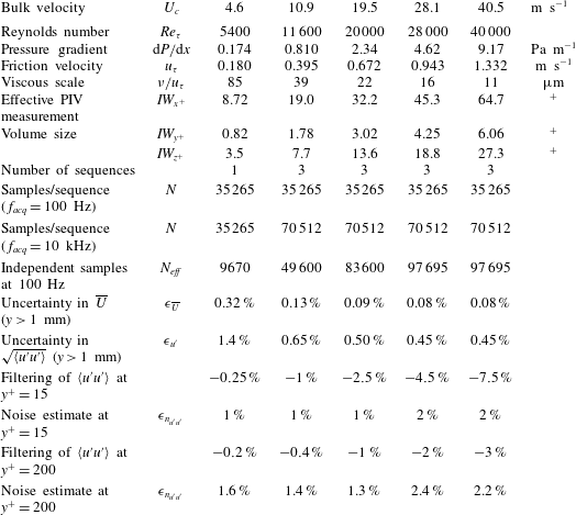
The PIV measurements were performed at five Reynolds numbers, as summarized in table 1, which also shows the details of the measurement volume for the PIV in viscous units, which, as already pointed out, was controlled by the laser sheet thickness, which was always smaller that the depth of field.
The PIV acquisition parameters for near-wall turbulent pipe flow measurements.

Statistically converged velocity profiles could be achieved using up to 70 000 samples per sequence acquired at low laser repetition rates (100 Hz). Higher sampling rates of 10 kHz provided temporally coherent data from which frequency spectra could be obtained.
With increasing Reynolds number (
 $U_{c}=30{-}40~\text{m}~\text{s}^{-1}$
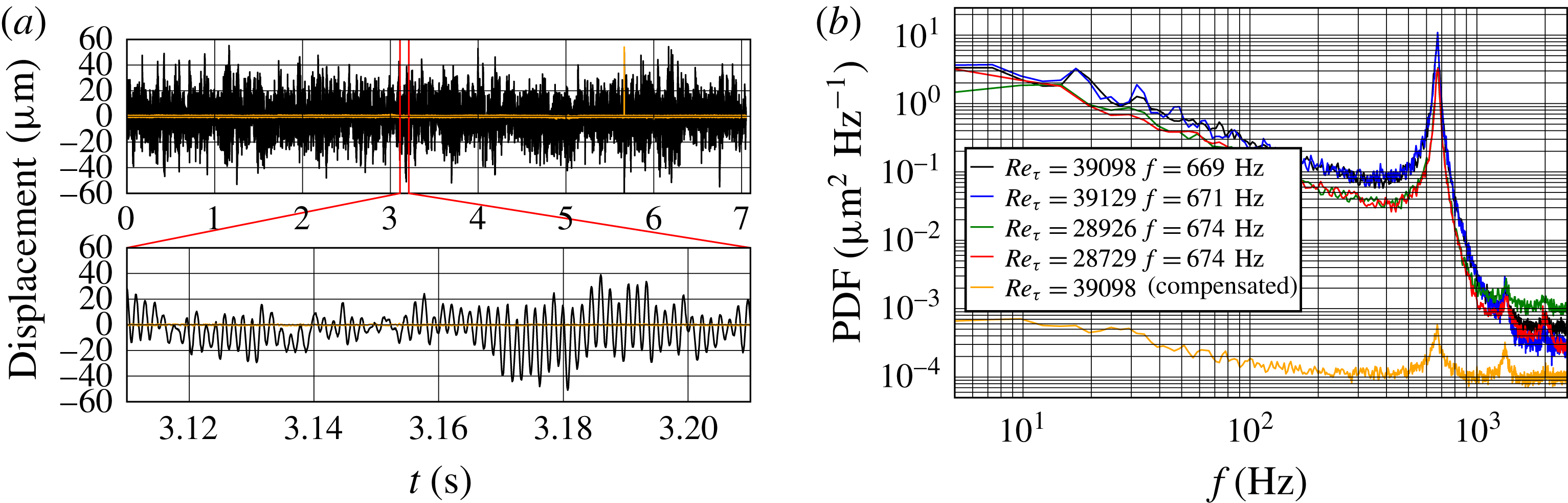
), a slight vibration was observed in the image data through a fluctuation of the wall position of up to 5 pixels peak to peak (
 ${\approx}50~\unicode[STIX]{x03BC}\text{m}$
) (figure 3
a). The vibration had a constant fundamental frequency of approximately 670 Hz throughout the duration of the measurement campaign and was found to be independent of the Reynolds number (figure 3
b). It was not possible, without further studies, to determine whether this small vibration was due to a vibration of the pipe structure or of the optical set-up, as both would result in the observed relative wall motion. Nonetheless, this offset must be accounted for prior to analysis to warrant reliable data in the immediate vicinity of the wall. Using an image correlation approach, the motion of the wall was tracked to better than
 $\pm 0.1$
pixel, i.e. better than
 $\pm 0.1\,^{+}$
at the highest Reynolds number. These displacement data were used to offset the images prior to PIV processing.
(a) The time trace of the detected vibration at
 $Re_{\unicode[STIX]{x1D70F}}\approx 40\,000$
acquired at 10 kHz. The orange line indicates the detected residual vibration after the image offset procedure. (b) Vibration spectra for different image sequences.

The image data were processed using a multigrid/multipass 2C–2D cross-correlation PIV analysis algorithm (Willert & Gharib Reference Willert and Gharib1991; Soria Reference Soria1996), with measurement volumes of 6 pixels in the wall-normal direction, corresponding to
 $0.8\,^{+}$
at
 $Re_{\unicode[STIX]{x1D70F}}=5400$
and increasing to
 $6.1\,^{+}$
at
 $Re_{\unicode[STIX]{x1D70F}}=40\,000$
. In the streamwise direction, the measurement volume had a length of 64 pixels (
 $700~\unicode[STIX]{x03BC}\text{m}$
), introducing minor spatial filtering, while in the spanwise direction, the measurement volume was controlled by the approximately
 $300~\unicode[STIX]{x03BC}\text{m}$
thin laser sheet, which also introduced minor spatial filtering. Full details of these measurement parameters and other pertinent experimental parameters are provided in table 1, and, as mentioned above, represent the highest-spatial-resolution
 $(u,v)$
near-wall velocity measurements for
 $Re_{\unicode[STIX]{x1D70F}}=5400{-}40\,000$
.
To support this argument, the missing energy due to PIV filtering was coupled to the finite-volume PIV interrogation, which was estimated with the 1D transfer function of PIV for the streamwise spectrum, as proposed by Foucaut, Carlier & Stanislas (Reference Foucaut, Carlier and Stanislas2004), applied to the hot-wire spectrum of the boundary layer obtained by Carlier & Stanislas (Reference Carlier and Stanislas2005). The difference in the integral of the filtered spectrum compared with the original one can be considered as the best estimation of the missing energy, and the result is given in table 1 for
 $y^{+}=15$
and 200. Also provided is the PIV noise part, which overestimates
 $\langle u^{\prime 2}\rangle ^{+}$
for these two wall-normal positions.
3 Results and discussion
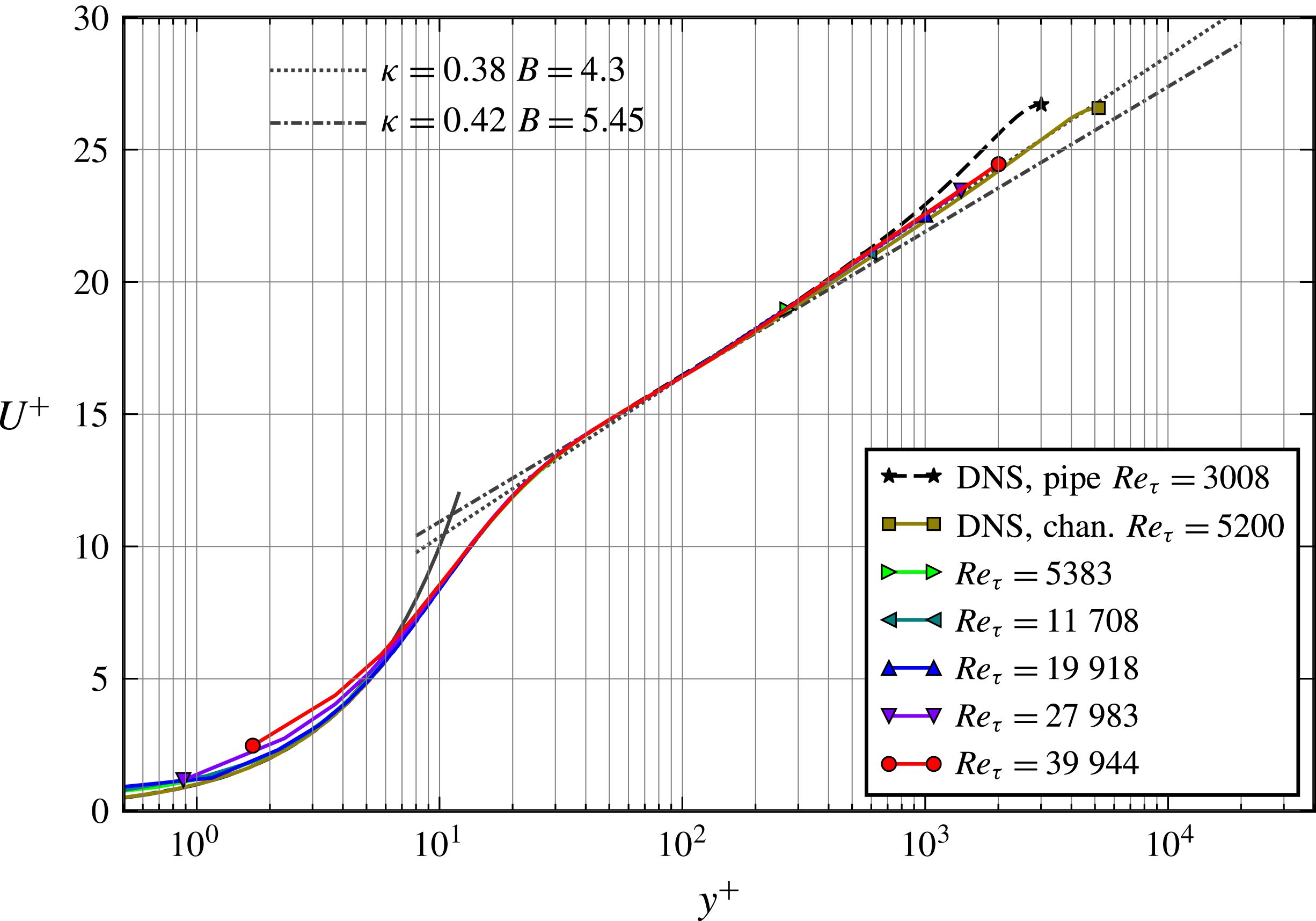
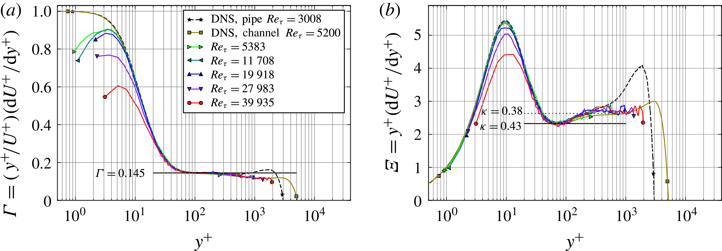
The profiles of the mean velocity and measured Reynolds stresses plotted in figures 4 and 5 respectively show that they only differ marginally from those of turbulent channel flows and flat-plate boundary layers from the wall up through the logarithmic layer. The mean streamwise velocity profiles are fairly consistent across all Reynolds numbers and in good agreement with the DNS channel flow results of Lee & Moser (Reference Lee and Moser2015). A clear log region is also observable. Figure 6 shows the indicator functions for a power law (a) and a log law (b). It does not show a consistently strict plateau region for either case. Although there is less scatter in the power law indicator function shown in figure 6(a), there is no horizontal plateau region for
 $y^{+}>200$
, and while the log indicator function has more scatter, an approximate plateau region is observable for
 $200<y^{+}<2000$
, which is consistent with the DNS channel flow results of Lee & Moser (Reference Lee and Moser2015), where an approximate plateau was found in the log indicator function between
 $y^{+}=350$
and
 $y^{+}=830$
.
Mean streamwise velocity scaled with inner variables; DNS of turbulent pipe flow at
 $Re_{\unicode[STIX]{x1D70F}}=3008$
by Ahn et al. (Reference Ahn, Lee, Lee, Kang and Sung2015) and DNS of turbulent channel flow data at
 $Re_{\unicode[STIX]{x1D70F}}=5200$
by Lee & Moser (Reference Lee and Moser2015).

(a) Variances and co-variances of the streamwise and wall-normal velocity components; DNS of turbulent pipe flow at
 $Re_{\unicode[STIX]{x1D70F}}=3008$
by Ahn et al. (Reference Ahn, Lee, Lee, Kang and Sung2015) and DNS of turbulent channel flow data at
 $Re_{\unicode[STIX]{x1D70F}}=5200$
by Lee & Moser (Reference Lee and Moser2015). (b) The variance of the streamwise velocity in comparison with NSTAP data obtained in the SuperPipe (Hultmark et al.
Reference Hultmark, Vallikivi, Bailey and Smits2013); all other symbols are as in figure 4.

As far as the Reynolds stresses are concerned, the data show a well-resolved inner peak of the streamwise velocity fluctuations
 $\langle u^{\prime 2}\rangle ^{+}$
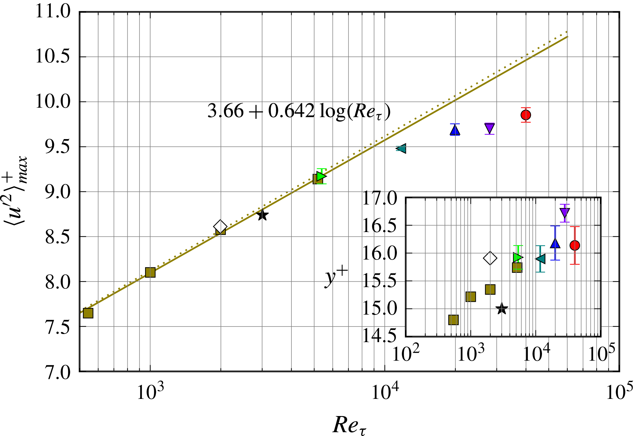
that grows with increasing Reynolds number (see the inset of figure 5), which so far has not been clearly documented in previous measurements of high-
 $Re$
pipe flows such as the Princeton SuperPipe (see, e.g., Hultmark et al.
Reference Hultmark, Vallikivi, Bailey and Smits2012; Vallikivi, Ganapathisubramani & Smits Reference Vallikivi, Ganapathisubramani and Smits2015), most likely due to lack of spatial resolution. For comparison, two profiles of the streamwise velocity fluctuations
 $\langle u^{\prime 2}\rangle ^{+}$
acquired in the SuperPipe using NSTAP hot-wire probes are presented in figure 5(b).
The PIV data also provide the wall-normal velocity component
 $v$
, from which two additional terms of the Reynolds stress tensor can be computed. Shown in figure 5(a), the plateaus of
 $\langle v^{\prime 2}\rangle ^{+}$
and
 $\langle u^{\prime }v^{\prime }\rangle ^{+}$
extend significantly with increasing
 $Re_{\unicode[STIX]{x1D70F}}$
, with the ends not captured due to the limited field of view.
The wall-normal distributions of the power law (a) and log law (b) indicator functions; DNS of turbulent pipe flow at
 $Re_{\unicode[STIX]{x1D70F}}=3008$
by Ahn et al. (Reference Ahn, Lee, Lee, Kang and Sung2015) and DNS of turbulent channel flow data at
 $Re_{\unicode[STIX]{x1D70F}}=5200$
by Lee & Moser (Reference Lee and Moser2015).

At
 $Re_{\unicode[STIX]{x1D70F}}=5400$
, both the profile and the maximum of
 $\langle u^{\prime 2}\rangle ^{+}$
or the inner peak match the DNS channel flow data at
 $Re_{\unicode[STIX]{x1D70F}}=5200$
by Lee & Moser (Reference Lee and Moser2015). Figure 7 shows that, with increasing
 $Re_{\unicode[STIX]{x1D70F}}$
, the maximum departs from extrapolations made from DNS channel flow data by Lozano-Durán & Jiménez (Reference Lozano-Durán and Jiménez2014) and Lee & Moser (Reference Lee and Moser2015) and for turbulent boundary layers by Sillero, Jimenez & Moser (Reference Sillero, Jimenez and Moser2014). The present data suggest a nonlinear trend of the inner peak magnitude with Reynolds number, which has to be taken with caution as the filtering effects increase with Reynolds number (
 $-5.5\,\%$
at the maximum
 $Re_{\unicode[STIX]{x1D70F}}$
studied).
Dependence of the variance maximum of
 $u$
on the Reynolds number
 $Re_{\unicode[STIX]{x1D70F}}$
and the wall-normal location of the maximum (inset). The squares (▫) and predicted relationship (solid line) from DNS are from Lee & Moser (Reference Lee and Moser2015), the dotted line is from Lozano-Durán & Jiménez (Reference Lozano-Durán and Jiménez2014), the stars (
 $\star$
) are from DNS of turbulent pipe flow at
 $Re_{\unicode[STIX]{x1D70F}}=3008$
by Ahn et al. (Reference Ahn, Lee, Lee, Kang and Sung2015) and the diamonds (♢) are from DNS of a turbulent boundary layer at
 $Re_{\unicode[STIX]{x1D70F}}=2000$
by Sillero et al. (Reference Sillero, Jimenez and Moser2014).

As far as the peak position of
 $\langle u^{\prime 2}\rangle _{max}^{+}$
with respect to the wall is concerned, the DNS predicts an increase with
 $Re_{\unicode[STIX]{x1D70F}}$
(inset in figure 7), which can be clearly observed in the present measurements. However, there is some scatter in the peak location due to the finite sampling spacing of 2.0 pixel in
 $y$
corresponding to
 $2\,^{+}$
at
 $Re_{\unicode[STIX]{x1D70F}}=40\,000$
. Finer spatial sampling and/or peak fitting may improve the estimates of both the position and the magnitude of
 $\langle u^{\prime 2}\rangle _{max}^{+}$
.
As shown in figure 5, although limited to the lower 20 mm of the pipe (i.e.
 $y/R\leqslant 0.044$
), the spatial domain of the present measurements is sufficient to also document the steady growth of the outer peak of the streamwise Reynolds stresses. A distinct outer peak clearly develops with increasing
 $Re_{\unicode[STIX]{x1D70F}}$
and is observable for
 $Re_{\unicode[STIX]{x1D70F}}\geqslant 20\,000$
. This outer peak is found to shift away from the inner peak with
 $Re_{\unicode[STIX]{x1D70F}}$
, a behaviour that is in good agreement with data acquired in the SuperPipe facility (Hultmark et al.
Reference Hultmark, Vallikivi, Bailey and Smits2012; Vallikivi et al.
Reference Vallikivi, Ganapathisubramani and Smits2015) (see also figure 5
b).
Consideration of the wall-normal distribution of the integral time scales of
 $U$
estimated through integration of the autocorrelation of the streamwise velocity (Pope Reference Pope2000) indicates that only the measurements for
 $Re_{\unicode[STIX]{x1D70F}}=30\,000$
and 40 000 are uncorrelated when acquired at
 $f_{acq}=100$
Hz. For all other sequences, the number of effective samples
 $N_{eff}$
is lower than
 $N_{tot}$
and is used for the uncertainty estimates provided in table 1. Following Benedict & Gould (Reference Benedict and Gould1996), the uncertainty of both the mean and the standard deviation of the streamwise velocity is based on a 95 % confidence interval, which is estimated from
 $N_{eff}$
and the estimated single-sample uncertainty of the measured velocity
 $\unicode[STIX]{x1D70E}_{u}$
at the 95 % confidence level using
 $$\begin{eqnarray}\unicode[STIX]{x1D716}_{\overline{U}}=\frac{1.96}{\overline{U}}\,\sqrt{\frac{\unicode[STIX]{x1D70E}_{u}^{2}}{N_{eff}}},\quad \unicode[STIX]{x1D716}_{u^{\prime }}=\frac{1.96}{\sqrt{\langle u^{\prime }u^{\prime }\rangle }}\,\sqrt{\frac{\unicode[STIX]{x1D70E}_{u}^{2}}{2N_{eff}}}.\end{eqnarray}$$
4 Concluding remarks
The combination of a facility offering relatively large viscous scales at high Reynolds numbers and a specifically adapted implementation of PIV enabled 2C–2D velocity measurements with high spatial and temporal resolution. This allowed, for the first time, a characterization of the near-wall velocity statistics of turbulent pipe flow at
 $Re_{\unicode[STIX]{x1D70F}}$
up to 40 000, which are beyond the reach of current DNS and thus far could not be resolved in other facilities operating at similar Reynolds number, due to the much reduced viscous scales present there. These new data acquired in the CICLoPE facility not only show the emergence of the outer peak, as observed in previous studies (e.g. Princeton’s SuperPipe), but also provide evidence of the persistence of the inner peak of the streamwise fluctuation, with a consistently higher amplitude than the outer peak. This inner peak is likely to continue to grow at even higher Reynolds numbers, and possibly not to be overtaken by the outer peak. In the near-wall region up into the logarithmic layer, the distribution of the streamwise variance is very similar to that of a flat-plate turbulent boundary layer. However, recent hot-wire measurements performed in the same facility show that, after applying a correction for lack of spatial resolution, the outer peak resembles a plateau more than a peak (Fiorini Reference Fiorini2017). Thus, although the present 2C–2D PIV measurements do not suffer to the same extent from spatial filtering, no firm conclusion about the existence and scaling of the outer peak can be made. However, it is found that the streamwise turbulent energy increases in this outer plateau or peak region with increasing Reynolds number.
As part of the EuHIT project, the data presented in this article will be made available on the EuHIT TurBase Knowledge Base (https://www.euhit.org/infrastructures/turbase-knowledge-base).
Acknowledgements
The authors would like to acknowledge the financial support provided through the ‘European High performance Infrastructures in Turbulence’ (EuHIT) Transnational Access Program (European Grant Agreement no. 312278). J.S. gratefully acknowledges the support of an Australian Research Council Discovery Outstanding Researcher Award fellowship. The visiting team would like to acknowledge the strong support and friendly atmosphere provided by the CICLoPE group during the entire test campaign (https://www.euhit.org/projects/HoloPipe).