1. INTRODUCTION
Building performance simulations are now commonly used by building professionals to test design alternatives before construction (Hong et al., Reference Hong, Chou and Bong2000). A large number of variables are included in most architectural designs, and many design solutions exist for given objectives. Learning about the relationships between potential design decisions and the desired performance could help designers achieve better design outcomes (Mackenzie & Gero, Reference Mackenzie and Gero1987). Traditional design activity is based on the assumptions and experiences that architects use to create and modify potential design solutions, in order to arrive at a design that is acceptable in both form and function. Usually the number of solutions an architect can create and evaluate within a reasonable timeframe is limited. Design by optimization effectively generates a large number of feasible solutions and pinpoints the best fitting ones for the specified design objectives. However, as we start to include building performance simulations into design optimization, the process becomes much more complex and time consuming.
Although building performance simulation and design optimization are powerful techniques for helping architects make better design decisions, they are very time consuming and require a significant amount of computing power. As a result, the integration of both techniques is unrealistic in real-world design practice; most projects simply have too tight a project timeline. Our research focuses on reducing the computing time in multiple-objective design optimization when building simulation techniques are involved. The methods used in this research not only facilitate a faster optimization but also enable a much larger search space within the same amount of time, which offers a better chance of finding the optimal design. The aim of this research is to encourage architects to use simulation and optimization in their daily practice. While improving today's practice is the ultimate goal of the project, the major contribution of the project is the future potential demonstrated by the present advancement of the optimization methods.
This research facilitates fast and extensive creation and evaluation of design alternatives through a process of searching, simulating, and optimizing, in order to meet specified architectural design objectives. It focuses on the early stages of the design decision-making process and is composed of the following computational methods: parametric modeling, performance simulation, multiple-objective design optimization, and genetic algorithms (GAs).
2. BACKGROUND AND LITERATURE REVIEW
2.1. Building performance simulation
With the growing demand for energy-efficient buildings, numerous building energy simulation tools have been developed. Green building standards such as LEED (USGBC, 2009) have been issued and implemented in many countries. A more sustainable and energy-saving type of design has been advocated by designers, engineers, and developers. The applications for building simulations include building heating and cooling load calculation, daylighting calculation and reflective roof analysis, building energy management and control system design, building regulations, code checking, cost analysis, and so forth (Hong et al., Reference Hong, Chou and Bong2000). Although many simulation tools exist today, the optimization process, which involves iterative simulations, is inefficient and time consuming.
2.2. Design by optimization and problem statement
Architectural design problems are generally complex and often involve multiple design objectives. Besides energy efficiency, other design objectives architects might consider throughout the comprehensive architectural design process include aesthetic, structural, functional, social, historical, behavioral, and so on (Lobos & Donath, Reference Lobos and Donath2010). Thus, architectural design can be seen as a multiple-objective optimization process, aiming to find optimal solutions for multiple objectives that often conflict with one another (Radford & Gero, Reference Radford and Gero1987). In general, there are two ways to solve multiple-objective optimization problems: convert a multiple-objective optimization into a single objective optimization by using a weighted sum of the objective functions with often arbitrary weights; or search for the Pareto optimal set, which is more widely accepted for practical multiple-objective optimization, because normally there exists a set of optimal solutions (design options) instead of a single solution for multiple-objective optimization. In this study we use the first method of design optimization. While the present methods can work for both of the two ways described above, in this study, we start testing our methods using the simpler way of optimization, converting a multiple-objective optimization into a single objective optimization. We will discuss the Pareto optimal optimization in a future study.
Because architectural design problems often having discrete, nonlinear, and stochastic decision variables, optimization methods such as classical calculus, linear programming, and dynamic programming are not applicable to most of the complex optimization problems in architecture (Radford & Gero, Reference Radford and Gero1987). GAs model natural selection and the process of evolution (Holland, Reference Holland1975). Using the mechanisms of natural selection in evolving individuals who adapt to an environment over time, GAs provide a robust search process and have been used in optimizing complex and poorly understood scientific and engineering problems (Gero & Louis, Reference Gero and Louis1995) such as automotive design (Vidal et al., Reference Vidal, Crainic, Gendreau, Lahrichi and Rei2012; Mahmoodabadi et al., Reference Mahmoodabadi, Safaie, Bagheri and Nariman-Zadeh2013), engineering design (Gen & Cheng, Reference Gen and Cheng2000; Deb, Reference Deb2012), medicine (Chen & Chen, Reference Chen and Chen2011), and so on. In the field of architecture, the applications for GAs include structural design (Kociecki & Adeli, Reference Kociecki and Adeli2013), green building design (Wang et al., Reference Wang, Zmeureanu and Rivard2005; Attia et al., Reference Attia, Gratia, De Herde and Hensen2012), and space planning (Jo & Gero, Reference Jo and Gero2006; Rawat et al., Reference Rawat, Shahani, Natu, Badami and Hingorani2012). Many tools (Gerber et al., Reference Gerber, Lin, Pan and Solmaz2012) are under development for the purpose of generation of design alternatives.
In addition to the improvement of multiple-objective GAs from the general computing point of view, there is a significant need to research a more efficient optimization tool that will couple with design simulations (e.g., energy simulations) more efficient during the optimization process. In this paper we present two proposed techniques for improving optimization as employed in a case study for space layout: an offline simulation technique, and a divide and conquer (D&C) method, customized for architectural design problems. The development of both methods is based on architects’ (as opposed to computer scientists’) domain of knowledge.
Time and computational complexity analyses are applied to evaluate an algorithm's usage of computing and time resources. A well-known limitation of GAs is that it often can take a tremendous amount of search and evaluation iterations before reaching optimal solutions, especially when the task involves multiple objectives. A GA optimization process could take days to complete using today's conventional computers. In an optimization study of insulation usage and space conditioning load, it took a GA 50 min to run 25 different designs and 2 h and 18 min to run 100 different designs on a standard laptop (1.7-GHz CPU, 512 MB RAM; Shi, Reference Shi2011). In a study of green building design optimization using multiple-objective GAs, a computer with Windows XP (3.06-GHz Pentium IV processor, 512 MB RAM) took 30 h to run 29 solutions (Wang et al., Reference Wang, Zmeureanu and Rivard2005). This time-consuming aspect of GAs could be a serious impediment to design automation, effectively discouraging designers from conducting more simulation studies. The number of generations and solutions in the above GA examples are too few to be of any practical use. When GA execution time can be saved by using a smaller search space, global optimality is unlikely to be achieved. In contrast, increasing GA search space to allow for a greater number of optimal solutions will result in a longer execution time, which in turn will prevent GAs from being useful in the design process. Thus, reducing the run time of GAs is essential to its use in design optimization.
Previous research studies have shown that building simulation is a very time-consuming and labor-intensive process. For instance, in a high-rise office building energy simulation study, the computer will need more than 30 h to perform a 1-year hourly simulation, and the time required for monthly simulations will vary from 36 min to around 6 h, using four desktop computers running at the same time (Ahn et al., Reference Ahn, Young-Jin, Deu-Woo, Sung-Hwan and Cheol-Soo2013). Researchers point out that the time and resources needed for simulation are one of the reasons that simulation tools have not been fully embraced by architects (Shi, Reference Shi2011). Architectural design firms have been using GAs as a way to search for the optimal design options to assist with the design decision-making process (Besserud et al., Reference Besserud, Skidmore and Merrill2008; Claussnitzer et al., Reference Claussnitzer, Katz, Shaxted, Park and Yori2014). However, due to the tight project timeline, architects do not have the time and resources. Most optimization projects have a small population. Therefore, the optimal solutions are not guaranteed to be found.
When a standard GA is used with simulation for optimization, a significant computer effort is expected (Renner & Ekárt, Reference Renner and Ekárt2003). As a result, various methods have been researched for increasing the speed of GAs. The literature on this topic can be divided into four groups. One involves improving the infrastructure, running GAs on a faster machine, or using multiple machines working together. The parallel GA uses a group of cooperating computers to solve complex problems in less time (Muhlenbein, Reference Muhlenbein and Rawlins1991). Cloud computing (Armbrust et al., 2000) has also been introduced as a way to reduce the computing time of optimization problems. Cloud services are now being used in many design firms to speed up the optimization process (Claussnitzer et al., Reference Claussnitzer, Katz, Shaxted, Park and Yori2014).
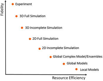
The second group of research in the literature investigates the construction of approximate simulation models: surrogate models. Surrogate models mimic the actual simulation model but use less computing power (Forrester et al., Reference Forrester, Bressloff and Keane2006). The computational cost of GAs can be reduced by replacing computationally expensive fitness evaluations with cheap approximation models such as surrogate models. (Ong et al., Reference Ong, Nair and Keane2003) A review paper (Jin, Reference Jin2005) points out that approximation models are beneficial when computation of the fitness function evaluation in GAs is time consuming; no analytical fitness function model exists (the fitness function needed to be evaluates by humans, for example, in music composition and art design); the results of GAs is not always consistent; and the fitness landscape has multiple local optimals. Surrogate models are used to replace the accurate and time-commuting fitness evaluation. It is recommended to use a surrogate model with the real/original fitness function to avoid having a false optimum in the surrogate model (Jin et al., Reference Jin, Olhofer and Sendhoff2000). The trade-off between the fidelity (approximation accuracy) and computational cost is shown in Figure 1 (Jin, Reference Jin2011). Generally speaking, fitness evaluations with high fidelity are more time consuming, and fitness evaluations with low fidelity are usually less time consuming. The user should balance between the needs for accuracy and available computational cost. Surrogate models are applicable to many operators in GAs. For example, population generation, crossover (Anderson & Hsu, Reference Anderson and Hsu1999), mutation (Abboud & Schoenauer, Reference Abboud, Schoenauer, Collet, Fonlupt, Hao, Lutton and Schoenauer2002), local search (Ong et al., Reference Ong, Nair and Lum2006), global search (Simpson et al., Reference Simpson, Mauery, Korte and Mistree2001), and fitness evaluations (Buche et al., Reference Buche, Schraudolph and Koumoutsakos2005; Jin, Reference Jin2011). Multiple surrogate models can be applied together to a GA problem. For example, researchers (Zhou et al., Reference Zhou, Ong, Nair, Keane and Lum2007) combine global and local surrogate models to improve the speed of an evolutionary optimization. However, surrogate models require simulation knowledge, that is, how to construct approximate simulation models, which architects usually do not possess. This inspired the present project in the reuse of offline or presimulation that architects already know how to conduct in the optimization process. The proposed methods are expected to be simpler for implementation than surrogate models because the original simulation models can be used in the optimization process.
The trade-off between fidelity and computational cost (adapted from Jin, Reference Jin2011).

The third group of research suggests to use simplified building simulation tools or reduce the number of simulation needs. Sentient building simulation systems construct a result database of a portion of the search space and interpolate the results based on designer's need (Negendahl et al., Reference Negendahl, Perkov and Heller2014).
The fourth group in the literature is focused on making the GAs work more efficiently. Associative parametric models can be used to describe a large and complex geometric system with fewer variables, which would make the optimization process faster (von Buelow et al., Reference von Buelow, Falk and Turrin2010). The evolutionary D&C algorithm reduces the complexity of the problem by dividing a large problem into simple subproblems (Valenzuela & Jones, Reference Valenzuela and Jones1993).
Based on the literature review, in order to improve a GA's application in architectural design, we first try to reduce the run time or the number of simulation runs in the optimization process; and second, we try to make GAs work more efficiently. In this paper we present two proposed techniques for improving optimization as employed in a case study for space layout: an offline simulation technique, which is a method to reduce the simulation needs, and D&C, which is a method to accelerate GAs, customized for architectural design problems. The development of both methods is based on architects’ (as opposed to computer scientists’) domain knowledge. The improvements can be additive to existing improvements, for example, the computing infrastructure improvements. Overall, this paper analyzes the existing problems and limitations of design optimization when associated with building simulation; presents the two proposed methods: offline simulation and D&C; and demonstrates a case study that could be used to validate these methods. This research also describes experiments performed on the use of parametric design, design optimization, daylight simulation, and design automation in the early conceptual design process.
3. METHODS
To reduce a GA's run time, we propose the use of offline simulation (Su & Yan, Reference Su and Yan2014) and D&C methods based on architecture's domain knowledge.
3.1. Offline simulation
In existing optimization processes, if building simulation programs are involved, simulations must be performed each time when the building parameters (chromosomes in the GA) change to form a new GA solution. The result of each simulation is used in the GA fitness function to produce another generation of solutions. This process continues until the GA finds the optimal solution or reaches a predefined calculation time limit. As a result, the simulation program must run until the GA finds the optimal solution. The number of simulations that need to be conducted is equal or proportional to the GA's population size.
In this research, we introduce the idea of offline simulation to reduce the number of simulations in the early stage of architectural design. Terms such as offline, online, or real-time have been widely used in engineering and scientific areas for physically based animation, physical system modeling, and simulation. Online or real-time simulation refers to a computer model simulation tool that works at the same rate as the actual physical system in a real-time clock. In other words, it will take the same amount of time in the real world for calculation in real-time simulation. Offline simulation tools usually work within a fixed time (Gole, Reference Gole2000).
In the domain of building design, offline and online concepts have been used in building system control design (Yu & Dexter, Reference Yu and Dexter2009; Coffey, Reference Coffey2012, Reference Coffey2013; Corbin et al., Reference Corbin, Henze and May-Ostendorp2013; Hu & Karava, Reference Hu and Karava2014). In the above literature, offline means that the optimizer is not connected with the server that controls the physical system (e.g., the physical building is not controlled by the optimizer). Online or real-time refers to the optimization process that connects the optimizer with a server–client framework controlling the building HVAC system (Corbin et al., Reference Corbin, Henze and May-Ostendorp2013). Hu and Karava (Reference Hu and Karava2014) simulated a mixed-zone building using offline model predictive control framework with particle swarm optimization as an optimizer. Coffey used offline optimization with building simulation tools to approximate model predictive control with lookup tables for optimal control setups. The results from offline optimization (the lookup tables) can be used in real-time building control simulations, so that the online optimization does not need to run at each time step. With offline optimization, online problems are easier to tackle, and simulations can be faster (Coffey, Reference Coffey2012, Reference Coffey2013). Similarity and difference lie between the above mentioned “offline” methods and the way we used offline in our study. The similarity is that the results from offline simulation can provide rules or knowledge for online systems later. The difference is in the work mentioned above, the offline optimization is separated from the real-time control of HVAC systems; in our study, the offline simulation is separated from the optimization process, and the simulation results can be used and reused in the optimization process later in the early stage of architectural design.
In conclusion, when the design problem is decomposable into subproblems where some subproblems can be solved offline, offline simulation/optimization methods can be used, making the original optimization problem easier to solve, reducing the computational time, and increasing the search space within the same amount of time.
Compared to real-time simulation, offline simulation in this study refers to a computer simulation model that can execute at a time different from that of the general GA optimization process. In order to save time, we separate building simulation from the GA optimization process, conduct all required simulations in advance, and reuse the simulation results whenever appropriate in the GA's fitness evaluation process. In other words, the correlations between building performance and decision variables can be obtained from offline simulations. These correlations can be used and reused in the GA fitness function. This way, simulations do not need to be repeated in the GA, and as a result, a significant amount of time can be saved.
3.2. D&C
The idea of the D&C technique is to divide a large problem into manageable subproblems. The solution to the original problem can be obtained by combining the solutions of the subproblems. This technique has the potential to be used in any complex optimization problem (Valenzuela & Jones, Reference Valenzuela and Jones1993). There are a number of different D&C methods already being used in the areas of mathematics and computing. For example, dynamic programming solves subproblems and combines the knowledge gained through the subproblems to reach the final solution; this process can be conducted without knowing how to decompose the original problem (Bellman, Reference Bellman1956). In the area of GAs, Potter and De Jong (Reference Potter, De Jong, Goos, Hartmanis and van Leeuwen1994, Reference Potter and De Jong2000) presented an evolutionary D&C technique called cooperative coevolution. In cooperative coevolution, the subcomponents are described as a collection of cooperating species. The individual species are coevolved and solved independently in order to solve a complex problem.
Prior work on engineering design has used multilevel hierarchical design optimization frameworks to solve large and complex design problems (Papalambros, Reference Papalambros2002) as well as a problem decomposition method, which is an analytic target cascading (Kim, Reference Kim2001; Kim et al., Reference Kim, Rideout and Papalambros2001). The benefits of the approach include efficiency, robustness, and organization.
In building design, analytic target cascading is extended to thermal and HAVC design (Choudhary et al., Reference Choudhary, Malkawi and Papalambros2003; Choudhary, Reference Choudhary2004; Choudary & Michalek, Reference Choudhary and Michalek2005). Different performance analysis goals may be involved in a complex design problem, which requires unique and separate analysis tools and optimization tasks in different levels of complexity (Choudhary et al. Reference Choudhary, Malkawi and Papalambros2003). The decomposition permits subproblems to be constructed separately, and allows appropriate simulation and optimization tools to be chosen from the tool repository and optimization to be conducted based on the individual performance objectives of the subproblems (Choudhary, Reference Choudhary2004). In terms of computational expense, simulation tools take the majority run time in this hierarchical framework; therefore; cheap simulation models are recommended (Choudhary, Reference Choudhary2004) and expensive models can be substituted by computationally cheap surrogate models (Papalambros, Reference Papalambros2002).
In Choudhary (Reference Choudhary2004) the problems are decomposed into subproblems using Object Decomposition (Wagner, Reference Wagner1993), which divides the problems by physical components such as zones and components, as well as Aspect Decomposition, which divides the problems by disciplines. While the idea of decomposing a problem into subproblems is similar in the D&C method, our study demonstrates a sequential object decomposition approach (decomposing the design problem into the layout optimization for patient rooms in sequence) that is applied to the process of GAs in the design of the spatial layout.
The idea of using a decomposition method to reduce the simulation time can also be seen in the work by Welle et al. (Reference Welle, Rogers and Fischer2012). The authors develop an automated method to decompose and recompose a building model for climate-based daylighting simulation, with great simulation time saving and simulation results that are acceptable. This method decomposes a building into many spaces and evaluates each space to check if it has distinct features and whether it should be simulated. A cloud computing platform then is used for simulations, and the results can be weighted and used for other spaces with similar characteristics. This decomposition method is used for daylighting simulation but not for optimization as in the present study.
The specific D&C method used in this paper, described by Watson (Reference Watson2002), is based on a decomposable and separable design problem. It is straightforward, easy to understand, and easy to conduct from the perspective of an architect. If the variables are independent from each other, for example, in simulations that usually use simplified models of the real-world design problems, we can break a design problem with a large number of populations into several subproblems, each with a smaller population, and solve them separately and with less time.
Suppose there are N variables in a complex optimization function F, and each variable has K possible values. If these variables are independent of each other (which means the value of one variable is not affected by the values of others), this problem can be broken down into N separable subproblems, each with only one variable. The function F can be expressed as the sum of N individual functions
 $$F({V_1}\comma{V_2}\comma \ldots\comma {V_N}) = {F_1}\lpar {{V_1}} \rpar + {F_2}\lpar {{V_2}} \rpar + \cdot \cdot \cdot + {F_N}\lpar {{V_N}} \rpar .$$
If we want to maximize/minimize the function F, we can maximize/minimize the functions F 1 to F N separately and with less computing time as described below.
In GAs, the computing time needed to solve the problem increases as the number of populations of candidate solutions increases. The D&C method decomposes a GA problem with a large population into several sub-GA problems with fewer populations. For a standard GA, the search space S standard is equal to the population size, which is
 $${S_{\rm standard}} = {K^N}.$$
For a GA using D&C, the search space is
 $${S_{\rm D\& C}} = N \times K$
and
 $$S_{\rm D\& C} = N \times K \lt \lt S_{\rm standard} = K^N\comma$$
especially when K and N are large. When the D&C method is applicable, the search space is much smaller. We can finish the algorithm with less computing time or enlarge the search space within the same timeframe. One requirement for the applicability of D&C is that the decision variables are independent of one another. In certain architectural design optimization problems, this requirement can be satisfied.
4. A CASE STUDY
4.1. Design objectives
Validations of the method is presented within the context of a case study for parametric form-finding in a nursing unit design with two design objectives: to minimize nurses’ travel distance from the nurses’ station to each patient room; and to maximize the daylight illuminance in all patient rooms, use LEED standard (healthcare supplement; USGBC, 2009) as a reference.
In any study related to the behavior and working efficiency of the nursing staff, one of the most important variables is the distance that a nurse is obligated to walk in a hospital. Walking has been identified as a major time-consuming activity for nurses, and evidence from previous studies suggests that the time saved by walking can be turned into more time spent on patient care activities (Zimring et al., Reference Zimring, Joseph and Choudhary2004). Individual nurses across all study units travel between 1 and 5 miles per 10-h daytime shift. Average travel distance ranges between 2.4 and 3.4 miles with a median of 3.0 miles per 10 h (Hendrich et al., Reference Hendrich, Chow, Skierczynski and Lu2008). Unnecessary walking may lead to time waste and add to fatigue and stress. In the case study, the objective is to minimize the total nurses’ walking distance.
Daylight is an essential element for patients’ well-being. Research shows that patients in sunny rooms feel less pain and stress, and take less medication as compared to patients in rooms with less sunlight (Walch et al., Reference Walch, Rabin, Day, Williams, Choi and Kang2005). This case study uses the LEED standard as a reference to construct the fitness function for the daylight illuminance level calculation (Rahmani Asl et al., Reference Rahmani Asl, Zarrinmehr and Yan2013). The objective is to achieve maximum daylighting under LEED requirement. LEED requires 75% or more of the perimeter area to achieve a daylight illuminance level between 110 and 5400 lux. Therefore, in this case study, the daylight illuminance in every inpatient unit layout design is expected to meet this requirement. The current tools and techniques used are introduced in Section 4.2, and the measurable baseline model is discussed in Section 4.3.
4.2. Design platform and tools
Parametric models can generate a very complex building geometry with a number of variables, rules, and constraints that are defined by the designers. Several design software tools offer parametric modeling features. Of these software options, the integrated Rhino/Grasshopper program has widely been used because of its powerful modeling capability, intuitive interface, and abundance of plugins that greatly expand its functionality. It also provides a ready-to-use GA plugin, Galapagos, which can be used for optimization. Hence, this case study uses Rhino/Grasshopper as the design platform. The following is a complete list of current tools and techniques used in this case study:
1. Rhinoceros (Rhino), a NURBS-based three-dimensional modeling program;
2. Grasshopper, a visual programming plugin for parametrically editing models in Rhino;
3. Galapagos, a GA tool in Grasshopper; and
4. DIVA, a thermal and daylight simulation plugin for Grasshopper. DIVA conducts daylight analyses for Rhino models through Radiance and DAYSIM daylight simulation engines.
The Galapagos-DIVA has been used in previous work for daylight analysis and optimization in the early architectural design process (e.g., Portugal & Guedes, Reference Portugal and Guedes2012; Gallas & Halin, Reference Gallas and Halin2013).
4.3. Baseline model
Here we present the simplified yet representative case study to validate the two methods we propose: offline simulation and D&C. The design problem is to find the optimal nursing unit layout that would allow for the least travel distance for nurses and a daylight illuminance that meets the LEED standard. The layout of the nursing unit is defined by a set of parameters, restrictions, and objectives. The parameters include constants and variables. The constants include a 15 × 15 grid with a total number of 225 cells, each measuring 15 × 15 ft. as possible room spaces; a central nurses’ station represented by the blue square, sized 29 × 29 ft.; an 8-ft. corridor outside of the central nurses’ station; the city of Boston as the location of the building in DIVA; and a window size of 6 × 6 ft. in every patient room. Figure 2 shows the constant parameters in a possible layout solution; the small red (dark) squares represent the patient rooms.
The constant parameters in a possible layout solution.

The variables are the locations of 12 patient rooms. A patient room can be located in any cell, with the following restrictions: a patient room cannot overlap with any other patient room, nurses’ station, or the corridor; and in order to introduce natural light into each room, a patient room cannot be surrounded by other rooms in all four directions. In other words, at least one of the four cells surrounding each room should be vacant for window opening.
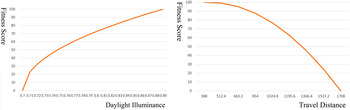
In this case study, we convert two objectives into a single objective by using a weighted sum of the objective functions with predefined (architects’ subjective) weights. For both travel distance and daylight illuminace, 100 points are given as the highest fitness score. The total nurses’ travel distance is calculated as the sum of the distances from the center of the central nurses’ station to the centers of all the patient rooms. The calculation of the nurses’ station to patient room distance and the total distance are simplified in the case study. In a practical situation, nurses’ walking distances are usually affected by the distance from the nurses’ station to the patient bed, following each nurse's travel path and affected by the order of that nurse's activities. Neither daylight nor travel distance subfitness functions should be linear in the overall fitness function. For daylight illuminance, losing the same amount of daylight affects more a darker room than a brighter room (Rutten, Reference Rutten2011; see Fig. 3 left). The same additional increment of travel distance makes a nurse feel much more fatigued, if that nurse has traveled a longer distance than someone who has just started a shift (see Fig. 3 right).
(Left) The daylight illuminance subfitness function is nonlinear. (Right) The travel distance subfitness function is nonlinear.

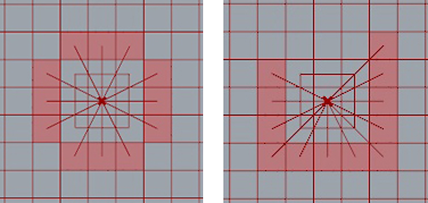
A fitness score of 100 is given to the nursing unit layout with the shortest total travel distance possible, 388 ft. (see Fig. 4, left), and 0 is given to the layout with the furthest total travel distance possible, 1,708 ft. (see Fig. 4, right). For any nursing unit layout solution, the fitness score for the travel distance is defined as follows. (We chose the power of 2 in the case study for simplicity of calculation.)
Unit layouts with the (left) shortest travel distance and (right) furthest travel distance.

 $$\eqalign{Fitness_{travel distance} & = 100 \left(1 - \left(\displaystyle{Distance - 388 \over 1708 - 388} \right)^{\!\!2} \right)\comma \cr & \qquad \le Distance \le 1708.}$$
Daylight illuminance is evaluated by the percentage of sensor grid points in a room achieving a daylight illuminance level between 110 and 5400 lux. In this case study, the above percentage is 89% if all rooms face south and 70% if all rooms face north (and in between for east and west). Fitness values of 100 and 0 are assigned to rooms with south-facing and north-facing windows, respectively. For any nursing unit layout solution, the fitness score for daylight illuminance is defined as follows:
 $$\eqalign{Fitnes{s_{daylighting}} & = 100 \left(Sqrt \left(1 - \displaystyle{{89\% - DaylightPercentage} \over {89\% - 70\%}} \right)\right)\comma \cr &70\% \le DaylightPercentage \le 89\%.} $$
According to LEED IEQ Credit 8.1 “Daylight and Views-Daylight,” daylight illuminance simulations should be conducted under clear sky conditions at two different times. In this research, those times are 9 a.m. and 3 p.m. on September 21. Thus, in DIVA, “clear sky with sun” and “illuminance” are selected for the sky conditions. However, DIVA can only conduct simulations at a specified time point in each run. In order to satisfy the LEED requirement, the optimization process must run two separate times, one on September 21 at 9 a.m. and the other at 3 p.m. Although the setup of both optimization processes have the same objectives and parameters (except the solar time) in DIVA, the results may be different because daylighting conditions differ. We perform both a 9 a.m. and 3 p.m. calculation in our case study.
The DIVA daylight simulation accuracy increases if more sensors are used in the patient rooms. However, the more sensors it uses, the more computing time it needs. Consequently, designers should balance the need for accuracy with the associated computing time, based on the project's requirements. In the baseline model used in this research, 100 sensors are evenly distributed in each room (1,200 sensors in 12 rooms total) at the level of desk height. All simulations are run on a standard laptop (ThinkPad series, Windows 7 64-bit, IntelR Core™ 2.50-GHz i5-2520M CPU with 8 GB of memory). In Galapagos, the population size per generation is 50, initial boost is 2, inbreeding factor is 75%, and maintain factor is 5%. For this particular study, a single run of the daylight simulation in DIVA requires approximately 1 to 2 min to complete. However, when DIVA is associated with Galapagos in the optimization process, it can be very time consuming; each solution requires a simulation. In our experiment, 78 h of DIVA run time + Galapagos could only calculate 13 generations of the GA, and the results were not nearly optimal in our examination. The complete optimization could take days, which is not practical even for this simplified case study.
Here, we summarize the problems we encountered during design optimization when using GAs and energy simulation as the platform. Due to the limitations of the software (Grasshopper + Galapagos + DIVA), only one specific time of a day (e.g., 9 a.m.) can be calculated per simulation. If design optimization involves a building simulation at a different time (e.g., 3 p.m.), the entire process must be reperformed. Thus, the information from both building simulations cannot be combined into one design optimization to find the optimal solution. Design optimization is very time consuming. Most architectural design projects have tight schedules. Therefore, it is unrealistic for architects to spend days on one optimization problem.
4.4. Offline simulation
Because the current design optimization process has the above-mentioned problems, offline simulation is introduced to integrate multiple building simulations at different times (e.g., 9 a.m. and 3 p.m.) into one optimization problem; and to reduce computing time when a building simulation is coupled with design optimization by separating the simulation from the optimization process. We separate the building simulation from the GA optimization process and conduct all required simulations in advance. This way, the simulation results can be reused in similar situations (e.g., all the rooms with windows facing the same direction will have the same daylight illuminance results in any GA generation and across the generations), and time-consuming simulations will not need to be run for each solution.
Because the locations of patient rooms are variables, one question is how to define the window opening directions. In terms of daylight, a very large window facing north and a relatively small window facing south might both satisfy the LEED daylight requirement. However, window-opening directions not only affect the interior daylight level but also have a significant impact on building energy consumption. In LEED, a project can earn up to 24 points in the “energy performance” category. The points that a building can earn depend upon the percentage of improvement in building energy consumption as compared to its baseline performance. This is calculated using a computer simulation model for the entire project based on Appendix G of the ANSI/ASHRAE/IESNA Standard 90.1-2007 (ASHRAE, 2007). The baseline model performance is defined as an average of the results of four simulations from four orientations: the original orientation of the building, and the orientation rotated by 90°, 180°, and 270°. The results of the thermal energy simulation using DIVA shows that the building consumes the least amount of heating and cooling energy when the window is facing south. The second best orientation is east, the third is west, and the worst is north. Based on this analysis, we conclude that the window-opening priority order should be south–east–west–north. Using this predefined priority list saves time spent computing the GA; if the priority list is not used, all possible directions must be included in the search space and evaluated by the simulation and fitness functions.
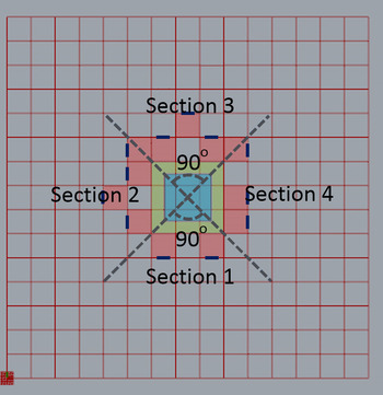
We divide the floor plan into four sections (see Fig. 5). A VB Script node written in Grasshopper is used to implement the following rules, the goal of which is to determine automatically each window's opening direction for the patient rooms during the GA process: if the center of a room is in Section 1, the priority of window-opening direction is south–east–west–north. VB will check the availability of adjacent rooms in the above sequence; if the center of the room is in Section 2, the priority is west–south–east–north; if the center of the room is in Section 3, the priority is north–south–east–west; if the center of the room is in Section 4, the priority is east–south–west–north. The center of a room is possible to be on a line that separates two sections. The priority rules for window-opening directions still hold in this situation: if the center of the room is on the line that separates Sections 1 and 2, or 1 and 4, the room has a south window; if the center is on the line that separates Sections 3 and 4, the room has an east window; and if the center is on the line that separates Sections 2 and 3, the room has a west window. Patient rooms are not required to be located next to the corridor. Any of the four directions of every room is possible for window opening, following the priority rules.
The floor plan is divided into four sections in order to determine the priority of window-opening directions. The windows’ locations are indicated in the figure as dark line segments on the edges of the rooms.

In more realistic simulations than this present, simplified study, further design modifications are required to make the design more practical in real projects: if the patient rooms are away from the corridor (not connected), additional corridors need to be added into the design layout; if the door of a room is blocked by other patient rooms, further modification to the design layout is needed. For example, in Figure 5, one room in the upper left corner needs access to the corridor.
One of the research questions can be stated as follows: because the parameters are consistently changing during the optimization process, how do we categorize the results of each simulation so that each category of simulation only needs a single simulation prior to the optimization process? For daylighting simulations, all patient rooms in this study share the same parameters (room dimensions, window size and location, building materials, number and location of sensors in DIVA), except for room locations and window-opening directions. However, as long as the patient rooms have the same window directions, the daylighting values of the rooms can be regarded as also being the same (in a simplified experiment, when shading is ignored). Based on this, the daylight simulations of all patient rooms in this project can be simplified as simulating four patient rooms with windows facing south, east, west, and north, respectively. Therefore, before the start of GA optimization, a DIVA daylight simulation is conducted to calculate the daylight level in every patient room. The location of rooms does not matter for daylight evaluation, only for walking distance calculation. The offline, presimulated daylight illuminance levels of all directions (south, east, west, and north) are used in the GA process. During the optimization process, although the room location and the window-opening direction may change in any design solution, we can obtain the daylight fitness score of the entire design solution by counting the total percentage of sensors that meet the LEED illuminance value.
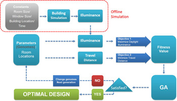
Comparing the workflows of existing design optimizations (see Fig. 6) and offline simulation-based optimizations (see Fig. 7), the difference is that in offline simulation-based optimizations, building simulations are performed prior to the optimization process. This change can reduce a significant amount of computing time. In this simplified case study, it took the computer approximately 40 min to calculate 13 generations of the GA when using the offline simulation method (plus about 8 min for the simulations of the four rooms with windows facing the four different directions), while the existing method uses 13 h for 13 generations of the GA. However, due to the large population size, although the obtained best nursing unit layout is close to the (perceived) optimal solution (an elliptical layout of patient rooms surrounding the nurses’ station), the improvement in solutions gets very slow after the 13th generation. Again, improvements to the GA process still need to be made.
The traditional genetic algorithm optimization workflow.

The improved genetic algorithm optimization workflow with offline simulation.

4.5. D&C
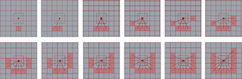
The method of D&C is evaluated here in an effort to further improve GA efficiency and save computing time. This method suggests the use of a GA to search in subproblems with fewer populations instead of the entire population. As mentioned in Section 3.2, one requirement for the applicability of D&C is that the decision variables are independent of one another. This requirement can be satisfied in the present case study. In this study, when all 12 genomes (room locations) are used in a GA, the total population size is 225 × 224 × · · · × 214 = 1.249 × 1028, where 225 is the number of possible locations for the first genome, 224 is the number of possible locations for the second genome after the first genome has selected a spot, and so on. However, if only one genome is used in one GA run, the population size can be reduced to 225 for the first room, 224 for the second room, and so on. The idea here is that instead of directly solving an optimization problem with 12 genomes, we solve another equivalent problem: optimizing one genome at a time for 12 times. Figure 8 shows the working process of the nursing unit layout optimization when applying the D&C method. Each time, one room is added to the previous result. This way, the nursing unit layout optimization is completed in 20 min.
The working process of the nursing unit layout optimization with the divide and conquer method.

When the D&C method is applicable, we can further improve the efficiency of the GA and simplify the GA coding by linking only one genome (the decision variable) to the fitness function. In this study, for the GA with the D&C method, the fitness function for the travel distance is as follows (the fitness function for daylighting remains the same in this study):
 $$\eqalign{Fitnes{s_{travel\,\,distance}} & = 100 \left(1 - {\left(\displaystyle{{Distance - 30} \over {143 - 30}}\right)^{\!\!2}}\right)\hbox{,} \cr &30\,ft \le Distance \le 143\,ft.}\hfill$$
5. RESULTS
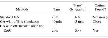
In this study, we convert a multiple-objective optimization into a single-objective optimization by using a weighted sum of the fitness functions with arbitrary weights. Figure 9 shows two optimization results with different weights in their fitness functions. The image on the left is the result when using equal weights for travel distance and daylighting. The image on the right is the result when the weights between travel distance and daylighting are 1:2. Although the optimal solutions are consistent with our intuitive expectations regarding the results, which is not surprising, the important point is the significant time savings when finding solutions with our new methods. Table 1 shows a comparison of the standard GA, a GA with the offline simulation method, and a GA with both the offline simulation and the D&C methods in terms of total time used, time used per generation, and whether the optimal solution is found. For this nursing unit optimization case study, using the existing method of GA optimization, the computer needs 78 h to finish 13 generations of GA calculation (6 h/generation), and the final result is not near optimal. By using offline simulation, the computing time is significantly reduced (to 40 min) to finish 13 generations of GA calculation (3 min/generation). However, even though 13 generations are not enough for finding the optimal layout, the result is close to optimal. To further reduce computing time, we experimented with the D&C method. This method provides a better chance of finding the peak of the fitness landscape by breaking a complicated problem down into subproblems. When we combine offline simulation and D&C in this project, no more than 24 generations in 20 min (50 s/generation) are needed to find the optimal layout (each subproblem's GA is stopped manually when no improvement is observed and therefore more generations are calculated than are necessary). In addition, the improved methods also help reduce the size and complexity of the model definition in the visual programming environment, Grasshopper.
The final results of the nursing unit layout optimization with different weights in the fitness functions: (left) fitness travel distance: fitness daylighting = 1:1 and (right) fitness travel distance: fitness daylighting = 1:2.

Comparison between standard GA and improved GAs

Note: GA, Genetic algorithm; D&C, divide and conquer.
6. CONCLUSIONS AND DISCUSSIONS
In this paper, we present two techniques (offline simulation and D&C) to achieve a more efficient GA optimization. The use of the two techniques demonstrates significant time savings in the case study and provides a larger GA search space in the same amount of time, which offer a better chance of finding the optimal design. The use of GA in architectural design has become a trend in design optimization. Currently, however, only the general method of GA has been applied to architectural problems. We have provided a new type of study that utilizes architectural domain knowledge to customize GA techniques, and as a result, we have significantly improved the design optimization time.
The reason for selecting a simplified case study is that it is useful to validate the methods and workflow. For a particular optimization problem, how do we verify that the results are the real optimized solutions, especially in healthcare design, when design problems are usually very complex and involve multiple design objectives? For these kinds of complex problems, the optimized solutions cannot be foreseen in order to verify the results. However, we can convert a complex problem into simplified versions of the original problem and experiment on the methods and workflow with the simplified problems. We can then verify the solutions for simplified problems by various techniques and thus verify the methods. In contrast, it is generally impossible to verify the solutions for a complex problem directly.
It is worth noting that the travel distance and daylighting performance were selected as the sample design objectives in this study among all quantifiable design objectives involved in nursing unit design, which include construction cost, energy consumption, equipment placement, and so on. Both objectives were chosen because (1) travel distance and daylighting are two of the most important concerns in nursing unit design and (2) travel distance and daylighting may have conflicting attributes because daylighting performance may decrease when travel distance is reduced (depending on the floor plan design), which needs to be confirmed by case studies. Both objectives can be substituted with other objectives because the focus of this study is the developing and testing of new optimization methods rather than studying the particular design objectives.
The tools used in this study, Rhino, Grasshopper, Galapagos, and DIVA, are widely available existing tools that facilitate the development of the present methods. The methods presented in this paper, however, are not tied to these tools. Instead, the methods can be applied to similar tools, and even new implementations of such tools in more efficient programming languages.
We can use the D&C method to reduce computing time in optimization problems when the original problem can be broken down into several manageable subproblems. In the case study, the D&C method required manual work to separately start the GA for each subproblem in sequence, due to limitations in the software. We expect future GA software products will be capable of automatically starting the GA for each subproblem in sequence. The offline simulation technique is beneficial when building simulations can be separated from the optimization process and conducted in advance. The simulation results can be reused in order to save computing time.
While we used simplified fitness functions for walking distance and daylighting performance, the daylighting simulation does not use surrogate models or approximate simulation models. Instead, offline or presimulation is used with the full daylighting simulation, and the reuse of the offline simulation results is conducted in the fitness functions of the optimization process. The simplified fitness functions can be substituted with more sophisticated fitness functions for different design objectives, but the method of reusing offline simulation in the process will remain the same for different design problems.
There are limitations in the use of the offline simulation and D&C methods. In offline simulation, the simulation result of each genome is precomputed, so there is no mutual feedback among genomes. For example, self-shading (e.g., a room may cast shadow to other rooms) is ignored in our simplified case study; thus, the effect of shading was not included in the daylight illumination result. If obstruction is considered in more complex spatial layouts, offline simulation may not be appropriate. One solution to this problem is to find and precompute all possible shading situations in advance. This may increase manual labor and computing time for offline simulation, but it can be assisted by scripting to automate the process. In a complex problem, designers may need to optimize the total GA computing and offline simulation time. The D&C method has a similar limitation. In D&C, a genome that is newly added into a GA has no impact on the genomes that have already been placed, but in actual problems, the genomes may be dependent (again, e.g., a room may cast a shadow to other rooms affecting their illumination). When genomes are not independent of one another, designers may group the subproblems into sets of subproblems to enable feedback among genomes within each set of subproblems. Future study is needed to further examine and resolve the limitations of both offline simulation and D&C.
To discover these improvement techniques, architectural domain knowledge was needed. For example, if two identical rooms (same shape, same windows, and same shading) in a building are facing the same direction, they have the same illuminance at any given time because the sun is far enough away that the difference in light angles between the two rooms is negligible. Another example is that in many cases in the Northern Hemisphere, the best window direction for optimal thermal performance is south, followed by east, west, and north. This knowledge was confirmed by our thermal simulation and used in the offline simulation. To sum up, designers can play an important role in improving optimization efficiency. We should utilize architects’ design knowledge to customize the optimization process, a process that would significantly save in computing time and eventually make optimization practical for architectural design.
In future work, the application of the methods to more complex case studies with more detailed building models and more sophisticated design objectives should be investigated. We will also expand these techniques to Pareto optimization for multiple design objectives. We will also investigate the utilization of more specific design knowledge, for example, evidence-based design knowledge found in research of healthcare facility design, and correlations or causal relationships among decision variables, among design solutions, and between decision variables and design solutions that can be acquired from building science, postoccupancy evaluation, and so on. When more specific or complex design knowledge is embedded into a GA and its improvement methods with more case studies, more interesting findings about the advantages and limitations of techniques such as offline simulation and D&C could be made. Guidelines can be developed about when the techniques can be utilized and what kind of design optimization problems can be applied.
Zhouzhou Su is a doctoral candidate in the Department of Architecture at Texas A&M University. She received her Bachelor's degree in architecture from Xi'an University of Architecture and Technology in China and her Master of architecture from Texas A&M University along with the Graduate Certificate in health systems and design. Her areas of interest include design optimization, parametric modeling, as well as healthcare facilities design and planning.
Wei Yan is an Associate Professor of architecture at Texas A&M University. He has a BE in architecture and ME in architectural science and technology from Tianjin University, a Postgraduate Certificate in CAAD from ETH Zurich, and an MS in computer science and PhD in architecture from the University of California, Berkeley. His research and teaching area is computational methods in architecture. His recent research has been funded by the NSF, NEH, DOE, ASHRAE, and Autodesk. Dr. Yan received a Best Paper Prize at the 2006 International Conference of Design Computing and Cognition, and he is a 2013 American Institute of Architects Latrobe Prize Finalist.