1 Introduction
Granular materials and other discrete media like foams respond differently from classical fluids to shear stresses. Rather than deforming uniformly, they indeed develop zones of intense shear (Nedderman & Laohakul Reference Nedderman and Laohakul1980; Desrues et al. Reference Desrues, Chambon, Mokni and Mazerolle1996; Mueth et al. Reference Mueth, Debregeas, Karczmar, Eng, Nagel and Jaeger2000; Darve et al. Reference Darve, Sibille, Daouadji and Nicot2007; Unger Reference Unger2007), i.e. shear bands neighboured by quasi-static regions or plug flows. These bands being characterized by important shear, material failure and an important dissipation of energy, their understanding is crucial to describe and predict granular flow onset and rheology, and has numerous applications for a wide range of applications in which granular transport is present (e.g. agricultural, civil engineering and geophysical processes).
The formation of shear bands in granular flows is often explained by the existence of a yield shear stress. In other words, the system cannot deform in steady state unless the stress applied to it overcomes a critical, finite value. At the grain scale, this property can be explained by the existence of a network of grain–grain interactions (Daniels Reference Daniels2017) that has to be broken for the flow to occur. The yield shear stress of a granular material is thus related to the strength of the contact network. Any continuum-like description of shear banding thus requires the transcription at the scale of the flow of the properties of the aforementioned network, which are grain-scale, or more precisely contact-scale, properties. This task is not trivial due to the inhomogeneous character of the force network in granular media which form filamentary force chains (Radjai et al. Reference Radjai, Jean, Moreau and Roux1996; Majmudar & Behringer Reference Majmudar and Behringer2005) obviously influenced by the geometrical arrangement of the grains. It should be noted that photoelastic force measurement (Owens & Daniels Reference Owens and Daniels2013; Daniels, Kollmer & Puckett Reference Daniels, Kollmer and Puckett2017) or acoustic methods (Zaitsev et al. Reference Zaitsev, Richard, Delannay, Tournat and Gusev2008; de Richter et al. Reference de Richter, Zaitsev, Richard, Delannay, Car and Tournat2010; Owens & Daniels Reference Owens and Daniels2011, Reference Owens and Daniels2013) are interesting and efficient techniques for quantifying the properties of the aforementioned force network.
The presence of interfaces is often neglected or minimized in the literature for the sake of simplicity, yet all the industrial applications and all the geophysical processes involving granular materials are bounded by at least one interface (e.g. sidewalls, bumpy bottom or erodible substrate). The effect of interfaces on the geometry of a static granular material is far from being negligible. It has indeed been known for decades that, due to the intrinsic steric hindrance of granular materials, the presence of interfaces induces modifications of the contact network that often propagate over distances of the order of several grain sizes (Verman & Banerjee Reference Verman and Banerjee1946; Ben Aïm & le Goff Reference Ben Aïm and le Goff1968), an effect diminished by the polydispersity and the angularity (Camenen, Descantes & Richard Reference Camenen, Descantes and Richard2012). Of course, these modifications will influence the force network in the granular material. As a consequence, interfaces between the studied system and boundaries may have a strong influence on the yield stress value and thus on shear localization (Ananda, Moka & Nott Reference Ananda, Moka and Nott2008). For example it has been shown that confined steady surface flows (Taberlet et al. Reference Taberlet, Richard, Valance, Losert, Pasini, Jenkins and Delannay2003, Reference Taberlet, Richard, Henry and Delannay2004; Jop, Forterre & Pouliquen Reference Jop, Forterre and Pouliquen2005; Crassous et al. Reference Crassous, Metayer, Richard and Laroche2008; Richard et al. Reference Richard, Valance, Métayer, Sanchez, Crassous, Louge and Delannay2008; Brodu, Richard & Delannay Reference Brodu, Richard and Delannay2013; Brodu et al. Reference Brodu, Delannay, Valance and Richard2015) and confined granular avalanches (Boltenhagen Reference Boltenhagen1999; Courrech du Pont et al. Reference Courrech du Pont, Gondret, Perrin and Rabaud2003; Métayer et al. Reference Métayer, Richard, Faisant and Delannay2010; Yang & Huang Reference Yang and Huang2016) are crucially influenced by the sidewalls. Shear cells (Kuwano, Ando & Hatano Reference Kuwano, Ando and Hatano2013; Moosavi et al. Reference Moosavi, Shaebani, Maleki, Török, Wolf and Losert2013) are also an interesting geometry to study the effect of interfaces on the shear localization. As an example, recently, using a torsional shear flow (Artoni & Richard Reference Artoni and Richard2018) or a rectangular parallelepiped periodic cell (Artoni & Richard Reference Artoni and Richard2015b ), Artoni & Richard have shown that shear localization can occur at several locations along the depth of the shear cell.
Here, we combine experiments, numerical simulations and a theoretical analysis to investigate granular flows in annular shear flow subject to a pressure at its top and for which the shear is induced by a rotating bumpy bottom. We study the internal stresses of granular systems in this geometry and quantify the effect of the stress heterogeneity induced by the sidewalls on the shear localization. This geometry is similar to that used in Savage & Sayed (Reference Savage and Sayed1984) and Wildman et al. (Reference Wildman, Martin, Huntley, Jenkins, Viswanathan, Fen and Parker2008) and more recently in Orlando & Shen (Reference Orlando and Shen2012, Reference Orlando and Shen2013). Note that a similar flow configuration has been recently used for segregation studies (Golick & Daniels Reference Golick and Daniels2009) in a shallow configuration which ensures a nearly linear velocity profile.
The paper is organized as follows. The next section (§ 2) is devoted to the description of the experimental set-up and measurement methods. The numerical methods are presented in § 3. The experimental and numerical results, respectively, are presented in §§ 4 and 5. Then § 6 focuses on a discussion in which a model capturing the reported results is presented. The final section (§ 7) presents our conclusions and looks towards future work.
2 Experimental set-up
2.1 Experimental shear cell and conditions
Experiments were performed with glass beads (
 $d=4$
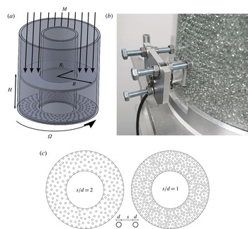
mm) in an annular shear cell (sketched in figure 1
a). The vertical boundaries of the cell consist of two coaxial cylinders made of poly(methyl methacrylate) (PMMA) having outer diameters of, respectively, 90 mm and 200 mm, and thickness of 5 mm, such that the internal spacing is
 $\unicode[STIX]{x0394}R=R-R_{i}=50~\text{mm}=12.5d$
. Such a spacing was chosen to limit the variation of velocity profiles with the radial coordinate. The horizontal boundaries are two (flat or bumpy) annular surfaces, which were made in poly(lactic acid) (PLA) with an FDM 3D printer in order to control the bumpiness. The bottom surface was screwed to a rotating plate, driven by a stepper motor (Lexium MDRive, Schneider Electric) between
 $\unicode[STIX]{x1D6FA}=1$
and 120 r.p.m. The top wall was fixed to a support, allowing it to move freely vertically but not to rotate, and where it was possible to load a certain number of steel masses, in order to apply a variable load to the granular material. The applied weight was varied between
 $M_{w}=0.22$
kg (corresponding to the bumpy wall plus the support without steel masses) and
 $M_{w}=5.4$
kg. The amount of glass beads in the cell was varied in the range
 $M_{g}=1.31{-}3.28~\text{kg}$
, corresponding to a range of bed height of 40–100 mm (
 $10d{-}25d$
). Also the effect of the bumpiness of the top and bottom walls was studied. In particular, three different surfaces were tested, two bumpy ones and a flat one, all of which were 3D printed in PLA. The bumpy walls consisted of flat walls on which hemispheres with diameter
 $d$
were deposited in a triangular mesh. Two values of the average distance
 $s$
between the borders of neighbouring asperities were tested, respectively,
 $s=1d$
and
 $s=2d$
(sketched in figure 1
c).
Details of the annular shear cell used in the experiments. (a) Sketch of the cell which is an annulus that confines the particles between a top plate free to move vertically but submitted to a force
 $Mg$
and a bottom plate rotating with an angular velocity
 $\unicode[STIX]{x1D6FA}$
. (b) Photo of the force sensor mount. (c) Sketch of the bumpy walls used for the top and bottom surfaces; the grain size is
 $d$
and the distance between neighbouring grains is
 $s$
.

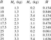
Table 1 lists the combinations of load and height for which velocity measurements were performed. In order to better understand the range of variation of parameters, some dimensionless parameters are introduced. The height is normalized with respect to the particle diameter
 $\tilde{H}=H/d$
, the applied weight with the mass of the grains
 $\tilde{M}=M_{w}/M_{g}$
, and the velocity of rotation by means of a Froude number defined by
 $Fr=\unicode[STIX]{x1D6FA}(R+R_{i})/(2\sqrt{gd})$
. The main tests were performed with bumpy walls with
 $s=2d$
. For each pair of
 $\tilde{H}$
and
 $\tilde{M}$
, three rotation velocities were tested,
 $\unicode[STIX]{x1D6FA}_{1}=5.9$
r.p.m.,
 $\unicode[STIX]{x1D6FA}_{2}=23.4$
r.p.m. and
 $\unicode[STIX]{x1D6FA}_{3}=117.2$
r.p.m., corresponding to a range in Froude number
 $Fr=0.2{-}4.3$
. For the other surfaces (flat and
 $s=1d$
) fewer tests were performed (load was varied between 1.0 and 5.4 kg, and the velocity was kept constant,
 $\unicode[STIX]{x1D6FA}=23$
r.p.m.).
Details of the experimental conditions. For each pair of combinations of flow depth normalized with respect to the grain diameter
 $\tilde{H}$
and applied load, three values of the Froude number were tested.
 $\tilde{M}$
is the ratio of the mass of grains
 $M_{g}$
to the applied mass
 $M_{w}$
.

In order to characterize the flow regime of our experiments and simulations, it is useful to introduce a dimensionless number, the inertial number, defined as
 $I=\dot{\unicode[STIX]{x1D6FE}}d/\sqrt{p/\unicode[STIX]{x1D70C}}$
(GDR-MiDi 2004), where
 $\dot{\unicode[STIX]{x1D6FE}}$
is the shear rate and
 $p$
is a pressure, while
 $\unicode[STIX]{x1D70C}$
is the density of the granular system. In our case, shear localization and the presence of stress profiles imply that
 $I$
varies with
 $z$
(and also slightly with
 $r$
for the experimental cell which is annular). The local inertial number range is between
 $10^{-5}$
(in the creep zone for low velocity and high load) and
 $10^{-1}$
(in the shear zone for high velocity and low load), which corresponds to the quasi-static and dense regimes of flow. Similar values are obtained in the numerical simulations (§ 3).
2.2 Velocity measurements
Velocity profiles were measured by cross-correlation particle image velocimetry (PIV) by recording the flow at the transparent outer cylinder. A high-speed camera was used (Phantom Miro 320S), and lighting was provided by two homogeneous light-emitting diode (LED) lamps (EFFILux EFFISharp) placed at each side of the camera. Given that a wide range of velocities were present (due to the variation of
 $\unicode[STIX]{x1D6FA}$
but more importantly due to the existence of creep zones), globally spanning over several orders of magnitude, for each test multiple movies were recorded at different frame rates, in order to have meaningful profiles for all the flow depth. The recorded zone width was around 50 mm, and the height of the window corresponded to
 $H$
; the resolution was
 ${\approx}10~\text{pixel}~\text{mm}^{-1}$
, and typical frame rates used spanned the range from 24 to 3400 f.p.s., while subsampling was also employed in some cases to obtain lower frame rates. In order to evaluate the relevance of a frame rate for a given vertical position, the theoretical displacement of particles between two successive frames based on the estimated velocity profiles was computed, and the frame rate was considered acceptable if the displacement was between 0.5 and 10 pixels. The final velocity profile was reconstructed by connecting the segments obtained at different frame rates, and eventually averaging superposing points. Cross-correlation PIV was performed in Python by using the package OpenPIV (http://www.openpiv.net/). All the procedure was verified against profiles obtained by manual tracking of some image sequences.
2.3 Force measurements at the wall
In addition to velocity measurements, forces at the outer cylindrical wall were also measured. For this purpose a six-axis force sensor (ATI Industrial Automation F/T Sensor Nano17) based on semiconductor strain gauges was used. The sensor was used to measure both normal and tangential forces at the wall. In order to do so, a square/rectangular window (
 $20~\text{mm}\times 20~\text{mm}$
) was laser cut from the outer cylinder, and fixed to the sensing head. The sensor was then mounted in correspondence to the window position and carefully adjusted in order to ensure the minimum discontinuity for the granular flow. An instruNet DAQ system was used for data acquisition at a frequency of 5 kHz. For converting voltages into force values, the calibration matrix provided by the vendor was used, after subtracting the offset determined with the sensor in place but without grains in the cell. The sensor calibration was verified with known masses.
Force measurements were carried out for the tallest granular flow (
 $\tilde{H}\sim 25$
); the experimental conditions correspond therefore to the last three lines in table 1. Three vertical positions of the sensing window were chosen:
 $h_{w}=15$
, 30, 70 mm (
 $h_{w}$
is the vertical position of the centre of the window from the bottom plate). The shape and dimension of the sensing window (
 ${\sim}5\times 5$
particle diameters), which was chosen based on compromises taking into account the force range measured by the sensor and the need for local measurements, imply that the values obtained for the forces are averaged on
 ${\sim}20$
particles and thus are not particle-scale forces.
In § 4, we will discuss results based on the average value of the forces exerted by the particles on the wall during the flow. Besides this, an analysis of the time evolution of the force signal was also performed. Autocorrelation was computed for each signal after removing peaks in the frequency spectrum related to disturbances induced by the motor. The autocorrelation time was estimated by integrating the autocorrelation function up to the first zero crossing. It appears (not shown here) that the autocorrelation time increases with
 $h_{w}$
and decreases with
 $Fr$
, which suggests that such a characteristic time is probably related to the time needed for a new particle to touch the sensor. It is important to recall that the dimension of the sensing window prevents insights from being obtained on the physics at the particle scale. The values of the autocorrelation time were therefore only used to guide the choice of the total recording time. The largest autocorrelation time (for the sensor at
 $h_{w}=70$
mm and the lowest velocity) was around 10 s; therefore force signals were acquired for 120 s, and three repetitions were made for each set of parameters.
3 Numerical simulations
3.1 Numerical method and set-up
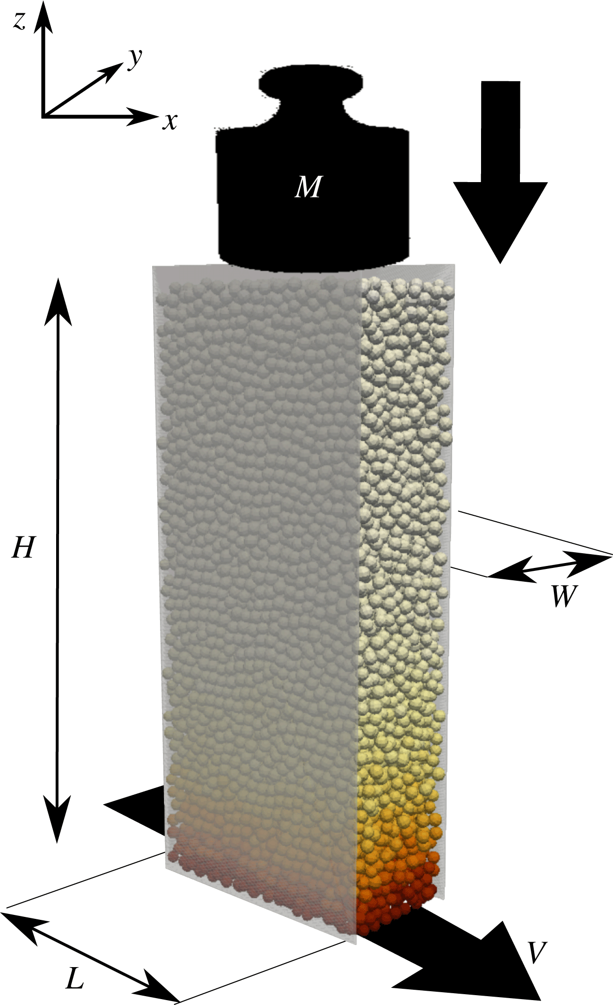
In order to better understand the dynamics of granular flow as highlighted by the experiments, discrete element method (DEM) numerical simulations were carried out. The flow configuration (sketched in figure 2, and which was previously discussed in Artoni & Richard (Reference Artoni and Richard2015b ), where some results were already presented) is a periodic rectangular cuboid in which shear is imposed by a bottom bumpy wall moving at fixed velocity, while a pressure is applied at the top bumpy wall; two flat but frictional sidewalls provide lateral confinement. The flow set-up is therefore a simplification of the experimental one, particularly removing the curvature of the flow.
Sketch of the numerical flow configuration, which is a shear cell bounded by flat frictional sidewalls normal to the
 $y$
direction and separated by
 $W$
. The
 $y=0$
plane is located at mid-distance between the two sidewalls. The height of the granular system is
 $H$
. The shear is imposed by a bottom bumpy wall moving at fixed velocity
 $V$
in the
 $x$
direction, which is periodic. A pressure
 $Mg/(LW)$
is applied at the top bumpy wall,
 $L$
being the size of the system in the streamwise direction.

Numerical simulations were carried out by means of the non-smooth contact dynamics method (Moreau Reference Moreau, Moreau and Panagiotopoulos1988; Jean Reference Jean1999), as implemented in the open-source platform LMGC90 (Renouf, Dubois & Alart Reference Renouf, Dubois and Alart2004). Gravity acts on the system along
 $z$
, and the flow is driven by the motion along
 $x$
of the bottom wall. The top wall cannot move in the
 $x$
and
 $y$
directions but is free to move in the
 $z$
direction, simply according to the balance between its weight and the force exerted by the grains. Sidewalls are separated by a distance
 $W=10d$
, and the periodic direction is characterized by a dimension
 $L=20d$
. Simulations were performed with
 $N=10\,000$
slightly polydisperse spheres (uniform number distribution in the range
 $0.9d{-}1.1d$
and with mean mass
 $m$
) interacting through perfectly inelastic collisions and Coulomb friction (
 $\unicode[STIX]{x1D707}=0.5$
). It has been shown that the coefficient of restitution has nearly no influence on dense granular flows due to the presence of enduring contacts (Dippel & Wolf Reference Dippel and Wolf1999). We therefore chose perfectly inelastic grains to maximize dissipation and thus save computation time. Interactions of particles with the flat walls were also perfectly inelastic and frictional (with a coefficient of friction
 $\unicode[STIX]{x1D707}_{pw}$
). The simulated cell is taller than the experimental one (
 $H\sim 45d$
). This was chosen for the purpose of studying the creep zone without the influence of the top wall. The bottom wall velocity was varied in the range
 $V=(0.1{-}10)\sqrt{gd}$
, the applied load (modelled as an added mass
 $M_{w}$
to the top wall) in the range
 $M_{w}=(0.2{-}2)M_{g}$
(where
 $M_{g}=Nm$
), and the particle–wall friction coefficient in the range
 $\unicode[STIX]{x1D707}_{pw}=0.05{-}0.3$
. The Froude number, defined in this case as
 $Fr=V/\sqrt{gd}$
, was therefore varied in the range 0.1–10. In this work the focus is on steady flows: this condition was assumed to hold when the kinetic energy was constant within the fluctuations. It is however important to note that the total kinetic energy may not be sufficient for characterizing the steady state in creep zones, because these contribute less than shear zones to the total kinetic energy. For this reason, after the total kinetic energy was stable, the system was sheared for an additional time, at least 10 times longer than the time of stabilization of the kinetic energy of the system, before taking averages. Depending on the simulation parameters, this corresponds to a total strain in shear zones of 4–1000; now, creep zones may be characterized by shear rates
 $10^{4}$
times smaller than shear zones. Therefore, notwithstanding the effort of applying a long pre-shear before averaging, for computational reasons in some cases the cumulative strain experienced by creep zones was only a few per cent. We nevertheless checked, in the averaging procedure, that no trend was present in the data, therefore supporting an assumption of stationary state.
3.2 Averaging method
In order to compute average profiles, several snapshots of particle positions and velocities were extracted from the simulations at different times. The data are both time- and space-averaged. Time averaging is obtained through a simple arithmetic mean over a number of snapshots (from 700 to 3000) which are taken at a time interval greater than the rearrangement time scale related to pressure (
 $d/\sqrt{p/\unicode[STIX]{x1D70C}}$
) and equal to
 $0.2\sqrt{d/g}$
.
Owing to the periodicity of the flow geometry, space averages were computed with respect to a grid in the
 $y{-}z$
plane; for each grid point the average velocity was computed by a space–time weighted average (Babic Reference Babic1997). In particular, an averaging method correctly computed velocity fluctuations with respect to the average velocity extrapolated at particle centres, as described by Artoni & Richard (Reference Artoni and Richard2015a
).
Given a particle-scale property
 $\unicode[STIX]{x1D713}_{p}(\boldsymbol{x}_{p},t^{\prime })$
, the mass-weighted space–time average
 $\bar{\unicode[STIX]{x1D713}}$
at point
 $\boldsymbol{x}$
and time
 $t$
is defined as (Babic Reference Babic1997):
 $$\begin{eqnarray}\unicode[STIX]{x1D70C}\bar{\unicode[STIX]{x1D713}}=\int _{-\infty }^{\infty }\mathop{\sum }_{p}w(\boldsymbol{x}_{p}-\boldsymbol{x},t^{\prime }-t)m_{p}\unicode[STIX]{x1D713}_{p}\,\text{d}t^{\prime }.\end{eqnarray}$$
Here
 $m_{p}$
is the mass of the particle;
 $w(\boldsymbol{x}_{p}-\boldsymbol{x},t^{\prime }-t)=w_{p}$
is a normalized weighting function evaluating the contribution of particle
 $p$
, at point
 $\boldsymbol{x}_{p}$
and time
 $t^{\prime }$
, to the average quantity
 $\bar{\unicode[STIX]{x1D713}}$
which is defined at point
 $\boldsymbol{x}$
and time
 $t$
; and
 $\unicode[STIX]{x1D70C}$
is the average density (obtained from coarse graining when
 $\unicode[STIX]{x1D713}_{p}=1$
). Applying this weighting function to the particle-scale equations of motion yields, after suitable manipulations, conservation equations for continuum-like variables in which classical terms such as contact and kinetic stresses, fluctuational energy fluxes and dissipation, etc. can be identified. (At least, this is the case for smooth particle interactions. For non-smooth interactions, such as in the present paper, the derivation of fluctuational energy balance terms from particle-scale equations requires a particular treatment. Nevertheless, the coarse-graining procedure detailed in Artoni & Richard (Reference Artoni and Richard2015a
) can be directly used to estimate solid fraction, average velocity, granular temperature, kinetic and contact stresses.)
Full expressions for the different variables can be found in Artoni & Richard (Reference Artoni and Richard2015a
). The weighting function can be seen as the product of two functions, respectively weighting in space and time:
 $w_{p}=w^{\prime }(\boldsymbol{x}_{p}-\boldsymbol{x})w^{\prime \prime }(t^{\prime }-t)$
. For space averaging, a number of coarse-graining functions have been tested in the literature, from a Heaviside step function to smoother ones like a Gaussian function. In this case, we follow Weinhart et al. (Reference Weinhart, Hartkamp, Thornton and Luding2013) by choosing a Lucy function, which in the present configuration takes the form
 $$\begin{eqnarray}w^{\prime }(r)=\frac{5}{\unicode[STIX]{x03C0}R^{2}l_{x}}\left(-3\left(\frac{r}{R}\right)^{4}+8\left(\frac{r}{R}\right)^{3}-6\left(\frac{r}{R}\right)^{2}+1\right),\quad \text{if}~r\leqslant R,\quad 0~\text{otherwise},\end{eqnarray}$$
where
 $r=\sqrt{(y_{p}-y)^{2}+(z_{p}-z)^{2}}$
, and
 $R$
is the coarse-graining cutoff radius (
 $R=d$
in the following). The compact support of the coarse-graining procedure is therefore a cylinder aligned with the
 $x$
direction. The prefactor ensures normalization, e.g.
 $\iiint w^{\prime }\,\text{d}\boldsymbol{x}=1$
. As regards time averaging, the weighting function can be defined in a similar way, and characterized by a time averaging scale
 $\unicode[STIX]{x1D70F}$
(which is the counterpart of
 $R$
). Depending on the nature of the flow, it is common to take
 $\unicode[STIX]{x1D70F}\rightarrow \infty$
, which means that time averaging is reduced to a simple average of space-weighted averages. If the flow is unsteady, however, this is not possible and the choice of
 $\unicode[STIX]{x1D70F}$
can be critical (Tunuguntla, Thornton & Weinhart Reference Tunuguntla, Thornton and Weinhart2016).
In the derivation of continuum balances from particle-scale equations of motion, the particle velocity fluctuations with respect to the mean field are introduced. In order to avoid the emergence of terms depending on the coarse-graining width
 $R$
, Artoni & Richard (Reference Artoni and Richard2015a
) have shown that the fluctuations have to be computed with respect to the space–time average velocity extrapolated at the particle centres, instead of that obtained at the averaging point. This yields consistent continuum level balances. While recognizing the importance of using an extrapolated average velocity, Zhang & Kamrin (Reference Zhang and Kamrin2017) claimed that such a coarse-graining method may include solid-like motions of rigid clusters of particles in the definition of the fluctuations, and therefore suggested that fluctuations have to be defined with respect to the instantaneous space average instead of the space–time one. In fact, this is not true for the coarse-graining method in general, but when
 $\unicode[STIX]{x1D70F}\rightarrow \infty$
is assumed, as discussed above. The definition of fluctuation of Zhang & Kamrin (Reference Zhang and Kamrin2017) is indeed consistent with the coarse-graining method of Artoni & Richard (Reference Artoni and Richard2015a
), when a Dirac delta function is chosen for
 $w^{\prime \prime }$
. From this discussion, we can state that in flows in which rigid clusters may form, the coarse-graining method is still valid, but
 $\unicode[STIX]{x1D70F}\rightarrow \infty$
may be questionable, depending on the meaning associated with the variables containing fluctuations. This is a delicate issue, however, given that choosing a Dirac delta function for
 $w^{\prime \prime }$
may end up – for example in situations in which space averaging cannot profit from periodicity – with coarse-graining supports containing few particles; this means that the averages might not be representative, and that may be a risk of underestimating velocity fluctuations. (In order to partially solve this problem, always considering the time scales of the phenomena in play, a good choice for the time averaging procedure could be some (intermediate) value of
 $\unicode[STIX]{x1D70F}$
operating a compromise between representativity of the averages and removal of solid-like fluctuations.) Moreover, this issue merits further analysis given that (1) solid-like fluctuations exist and definitely play a role in the flow, and (2) performing averages on instantaneous velocity profiles leads to neglecting time fluctuations of the flow (large eddies for example). If such correlated motions may not seem to cope with the concept of ‘fluidity’, they participate in different ways to balances (for example by dissipating energy at boundaries). Therefore, in this paper, we consider as a definition of granular temperature that based on fluctuations with respect to the time-averaged velocity, but we computed also the version based on instantaneous averages in order to understand the importance of collective motions on the flow. A detailed study on the different definitions of fluctuations is ongoing and will be the subject of future contributions.
Coarse-graining methods require particular attention when applied to near-wall regions. For example for stresses, Weinhart et al. (Reference Weinhart, Thornton, Luding and Bokhove2012) have shown that boundary interactions may be separately treated by the inclusion of boundary traction terms in the coarse-grained momentum balance equation. In our case, we include the boundary traction into the definition of stress. Near flat boundaries, variables such as velocity, solid fraction, kinetic stresses and granular temperature are estimated by renormalizing the weighting function by its integral on the portion of the compact support residing in the flow domain. In such a case the coarse-grained variables have to be considered to refer to the centre of mass of the averaging region based on corrected compact support, and not to the original grid point (Artoni & Richard Reference Artoni and Richard2015a
). Average wall stress profiles at lateral walls are simply estimated by summing the forces acting on
 $1d$
-wide horizontal stripes at different vertical positions and dividing the result by the area of the stripe (
 $Ld$
), after which simple time averaging is carried out.
4 Experimental results
4.1 Velocity profiles
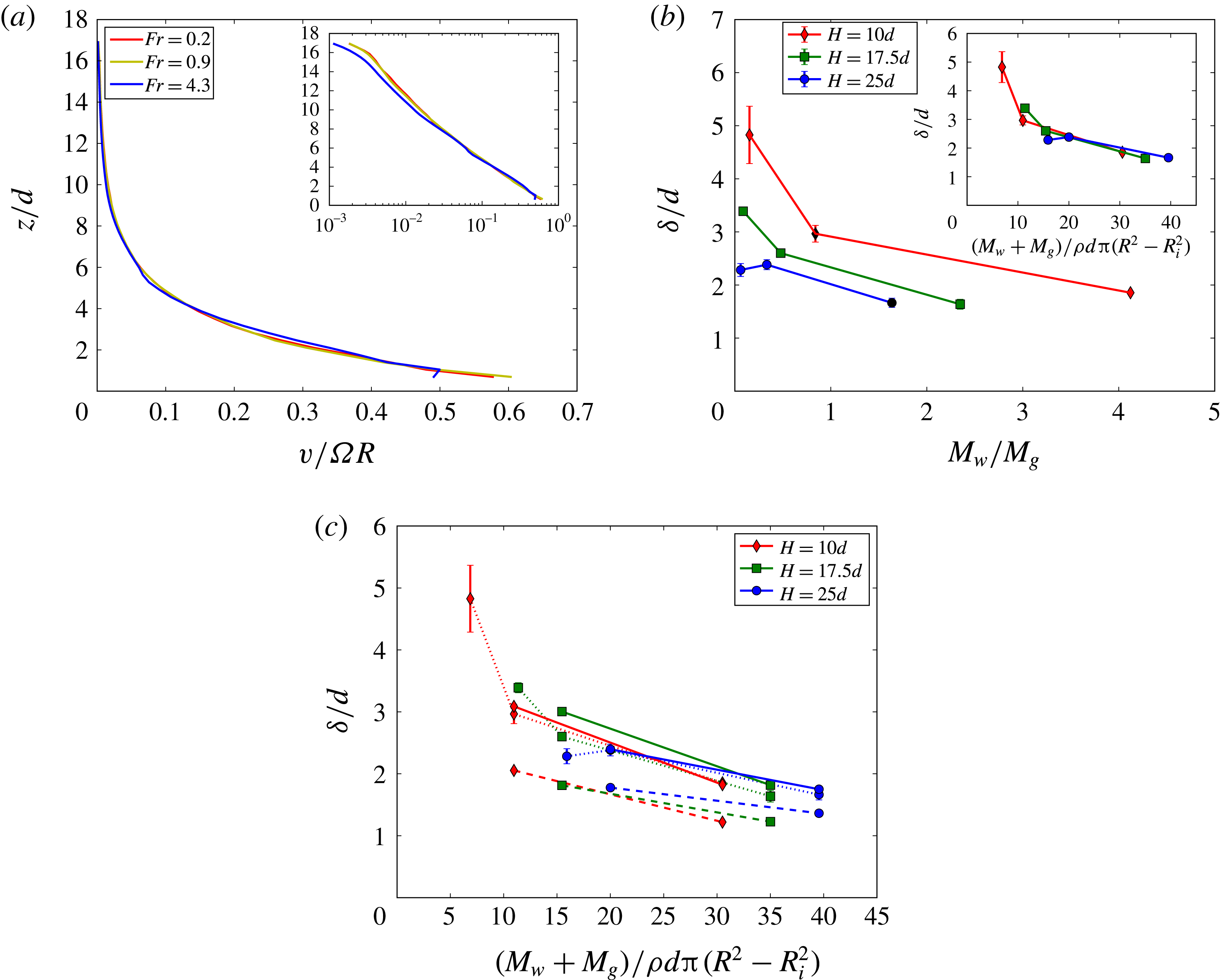
(a) Horizontal velocity profiles along
 $z$
measured by PIV from images captured at the outer wall for
 $\tilde{H}=17.5$
,
 $\tilde{M}=0.478$
(bumpiness
 $s=2d$
) and three values of the Froude number. (b) Decay
 $\unicode[STIX]{x1D6FF}$
of the velocity profile estimated from an exponential fit for different values of
 $\tilde{M}$
and
 $\tilde{H}$
, for the bumpy boundaries with
 $s=1d$
. Each point corresponds to the average of
 $\unicode[STIX]{x1D6FF}$
for three values of the Froude number. The inset shows that the results collapse when
 $\unicode[STIX]{x1D6FF}/d$
is plotted versus the dimensionless parameter
 $M_{w}+M_{g}/[\unicode[STIX]{x1D70C}d\unicode[STIX]{x03C0}(R^{2}-R_{i}^{2})]$
. (c) Effect of wall roughness on
 $\unicode[STIX]{x1D6FF}$
: smooth walls (dashed lines), intermediate bumpiness (
 $s=2d$
, dotted lines), highest bumpiness (
 $s=1d$
, solid lines).

Sample velocity profiles for the configuration with bumpy walls with
 $s=2d$
are displayed in figure 3(a). It is clear that, at least far from the top wall, velocity profiles display shear localization characterized by an exponential decay with
 $z$
. For this reason, in the following we characterize the profiles by means of a fit to an exponential function
 $v(z)=v_{1}+(v_{0}-v_{1})\exp (-z/\unicode[STIX]{x1D6FF})$
, and study the effect of process parameters on the decay length of the profile, given by
 $\unicode[STIX]{x1D6FF}$
. The parameter
 $v_{1}$
is needed for fitting given that a slight slip at the top was present in some cases. The parameter
 $v_{0}$
corresponds to the velocity of the bottom wall located at
 $z=0$
. Another point which is visible in figure 3(a) is that, once rescaled by the velocity of the bottom wall, profiles do not depend on the Froude number, at least for the studied range. This result is common to other granular flows, such as for example the vertical chute (Artoni, Santomaso & Canu Reference Artoni, Santomaso and Canu2007), where the shear band width appears to be independent of the flow rate. This feature of granular flows has been proven to be a failure point for local rheologies (Pouliquen et al.
Reference Pouliquen, Cassar, Forterre, Jop and Nicolas2006): this suggests that the present flow configuration might be an interesting benchmark for developments on the rheology of dense granular flows. Note however that, since we focus on relatively dense flows, one can expect an effect of the Froude number as the velocity is increased and the flow is more collisional. With this in mind, it is interesting to have a look at the joint effect of load and flow depth on the parameter
 $\unicode[STIX]{x1D6FF}$
, as shown in figure 3(b).
The first important result is that the decay of the profile is not universal but depends on the flow parameters. In particular, increasing the load induces a strengthening of the shear localization with a steeper decay, and increasing the flow depth seems to act in the same sense. In the limit of low load and shallow flow, the velocity profile is nearly linear. On the other hand, for the deepest flow considered (
 $\tilde{H}=25$
), the load has nearly no effect on
 $\unicode[STIX]{x1D6FF}$
, and for high load the effect of flow depth seems to be negligible. In other words, there seems to be a lower limit for
 $\unicode[STIX]{x1D6FF}$
which can be reached by increasing both the applied load and the flow depth. The inset of figure 3(b) shows that the results collapse reasonably well when
 $\unicode[STIX]{x1D6FF}/d$
is plotted versus a dimensionless parameter comparing an estimate for the pressure at the bottom wall (
 $(M_{w}+M_{g})g/[\unicode[STIX]{x03C0}(R^{2}-R_{i}^{2})]$
) to the pressure scale related to the mass of a grain (
 $\unicode[STIX]{x1D70C}gd$
). It seems therefore that, when the pressure at the bottom is low enough, shear can loosen the packing and extend over several particle diameters; otherwise, if the pressure at the bottom is high with respect to that induced by one grain, shear localization is enhanced and
 $\unicode[STIX]{x1D6FF}$
tends to a minimum asymptotic value.
Figure 3(c) shows the effect of the (top and bottom) wall texture on the bulk shear in the material. The highest bumpiness (
 $s=1d$
, solid lines) yields velocity profiles decaying approximately in the same way as the intermediate bumpiness (
 $s=2d$
, dotted lines, which are the same data as in figure 3
b). The smooth walls yield a value of
 $\unicode[STIX]{x1D6FF}$
that is slightly lower. Therefore the nature of the walls influences the shear localization features, even if not in a strong way. This can probably be ascribed to the flatness of the wall; in bumpy walls, the asperities probably enhance the geometrical frustration of the flow, increasing the zone affected by shear.
4.2 Force profiles
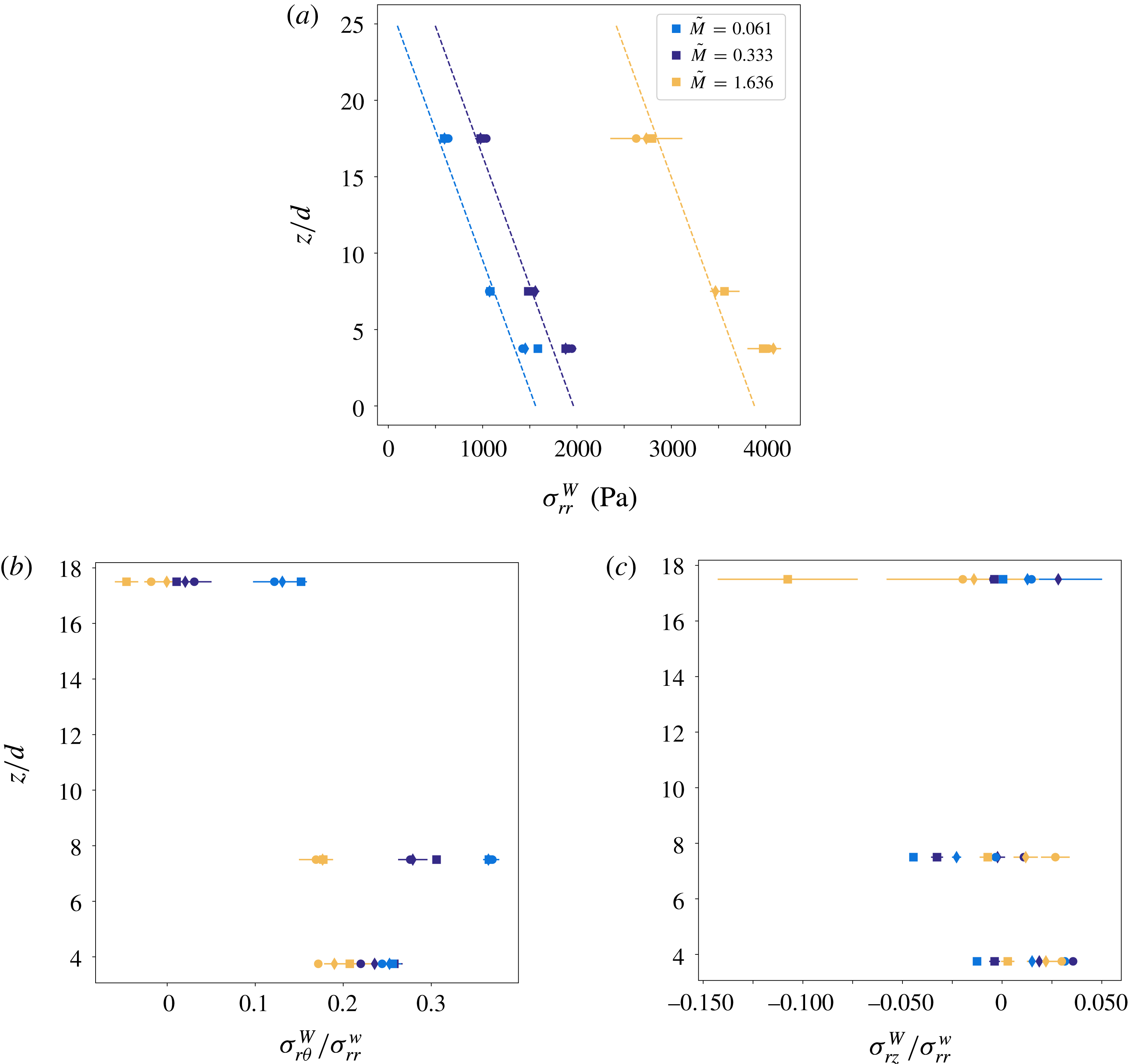
Results obtained from force measurements are displayed in figure 4. We particularly focus on the effect of
 $z$
, applied load and Froude number on the normal stress at the wall and the effective streamwise and transverse friction coefficients. We first look at the wall-normal stress
 $\unicode[STIX]{x1D70E}_{rr}^{W}$
(figure 4
a). Profiles are compared to a hydrostatic pressure profile
 $p=\unicode[STIX]{x1D70C}_{b}g(H-z)+M_{w}g/S$
, where
 $\unicode[STIX]{x1D70C}_{b}=M_{g}/(SH)$
is the average bulk density in the cell, and
 $S=\unicode[STIX]{x03C0}(R^{2}-R_{i}^{2})$
. It is clear that the hydrostatic profile captures quite well the decrease of stress with
 $z$
and the effect of the applied load. The measured stress is nevertheless slightly higher than the hydrostatic estimate for the position close to the bottom wall (as will be discussed in the following, this can be explained by lateral friction). Finally, the data allow one to state that the Froude number has nearly no influence on the normal stress for the range of parameters considered in this work.
Force measurements at different vertical positions on the external sidewall, for
 $\tilde{H}=25$
, intermediate bumpiness
 $s=2d$
, three values of the applied load, and three values of the Froude number (
 $Fr=0.2$
(circles), 0.9 (diamonds) and 4.3 (squares)). (a) Wall-normal stress
 $\unicode[STIX]{x1D70E}_{rr}^{W}$
versus
 $z$
; the dashed lines represent a theoretical hydrostatic pressure profile. (b) Effective, streamwise, wall friction coefficient
 $\unicode[STIX]{x1D70E}_{r\unicode[STIX]{x1D703}}^{W}/\unicode[STIX]{x1D70E}_{rr}^{W}$
. (c) Effective, transverse, wall friction coefficient
 $\unicode[STIX]{x1D70E}_{rz}^{W}/\unicode[STIX]{x1D70E}_{rr}^{W}$
.

From the other components of wall stress measured by the sensor, we can compute two effective wall friction coefficients: the streamwise,
 $\unicode[STIX]{x1D70E}_{r\unicode[STIX]{x1D703}}^{W}/\unicode[STIX]{x1D70E}_{rr}^{W}$
, and the transverse one,
 $\unicode[STIX]{x1D70E}_{rz}^{W}/\unicode[STIX]{x1D70E}_{rr}^{W}$
. The profiles of the streamwise wall friction coefficient (figure 4
b) are very interesting. This parameter is not at all uniform in
 $z$
, but, depending on the other parameters, may display first an increase from the first to the second point and then a decrease; increasing the applied load has the effect of decreasing the effective wall friction (down to nearly zero for the maximum applied load), and the Froude number has nearly no effect. The decrease in
 $\unicode[STIX]{x1D70E}_{r\unicode[STIX]{x1D703}}^{W}/\unicode[STIX]{x1D70E}_{rr}^{W}$
from the higher-shear region to the creep zone near the top is a signature of friction weakening (Richard et al.
Reference Richard, Valance, Métayer, Sanchez, Crassous, Louge and Delannay2008), which is clearly related to friction not being fully mobilized in creep motions. The non-monotonic behaviour of
 $\unicode[STIX]{x1D70E}_{r\unicode[STIX]{x1D703}}^{W}/\unicode[STIX]{x1D70E}_{rr}^{W}$
near the bottom, which is more evident for low
 $\tilde{M}$
, is more difficult to explain.
The transverse wall friction coefficient,
 $\unicode[STIX]{x1D70E}_{rz}^{W}/\unicode[STIX]{x1D70E}_{rr}^{W}$
, shows a more complex behaviour. The coefficient may be negative (if the average force exerted by the grains on the wall is oriented downwards) as well as positive (if the grains induce an upward-oriented force). Results suggest that the transverse friction coefficient is sensitive to both the Froude number and the applied load. However, for
 $z/d<8$
, it is definitely lower than its streamwise counterpart, clearly because the higher-shear region is characterized by a continuous horizontal flow of grains, which reduces the importance of vertical forces. For the highest probe point, which is characterized by a slow creep motion, the sign of the coefficient depends clearly on the applied load (with high
 $\tilde{M}$
inducing
 $\unicode[STIX]{x1D70E}_{rz}^{W}/\unicode[STIX]{x1D70E}_{rr}^{W}<0$
), and even if the values taken by this parameter are not large, one must consider that they are quite comparable to the streamwise coefficient. It is also evident that friction is not fully mobilized not only horizontally, but also vertically.
5 Numerical results
As detailed in the previous section, experimental velocity profiles in the annular shear cell are characterized by an exponential decay with
 $z$
which depends on the load and surface properties of the moving wall. Wall-normal stresses are roughly hydrostatic, while the streamwise effective friction coefficient displays weakening in the creep zone. In order to better understand the shear localization patterns and study the effect of the wall friction coefficient on the flow, discrete numerical simulations results are discussed in the following.
5.1 Kinematics
Velocity and granular temperature profiles are averaged in the
 $y$
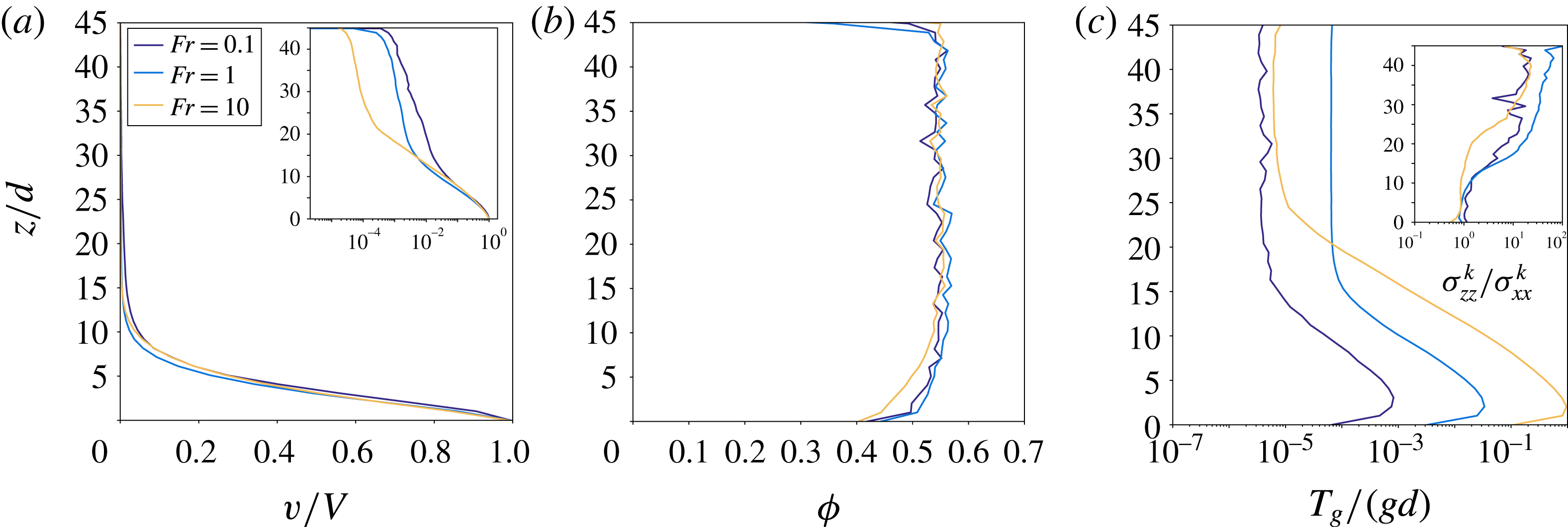
direction. Figure 5(a) displays numerical velocity profiles obtained for
 $\unicode[STIX]{x1D707}_{pw}=0.3$
. It is evident that the flow displays shear localization, with an exponential decay of the velocity with
 $z$
from the bottom wall. When profiles are rescaled by the velocity of the bottom wall, it is also evident that they are only slightly influenced by the Froude number – for the studied range – particularly in the high-shear zone. These two features are in agreement with the experimental results, and thus provide a qualitative validation to our simulations. The deviation from simple exponential decay which is observable in the creep zone in figure 5(a) may be ascribed to apparent slip at the top, another feature which was observed in experiments too.
Kinematic profiles in
 $z$
from numerical simulations (averaged in the
 $y$
direction), for
 $\unicode[STIX]{x1D707}_{pw}=0.3$
,
 $\tilde{M}=0.2$
and three values of the Froude number. (a) Streamwise velocity rescaled by the velocity
 $V$
of the bottom wall (the inset is the same but with the
 $x$
axis in log scale). (b) Solid fraction. (c) Granular temperature (inset: ratio between the vertical and horizontal normal kinetic stresses).

Solid fraction profiles for
 $\unicode[STIX]{x1D707}_{pw}=0.3$
(figure 5
b) are characterized by a uniform rate-independent value far from the bottom wall, and decrease when approaching the bottom boundary, with the highest velocity displaying larger dilatancy.
Effect of the definition of velocity fluctuations on granular temperature profile for
 $\tilde{M}=0.2$
,
 $\unicode[STIX]{x1D707}_{pw}=0.3$
and
 $Fr=1$
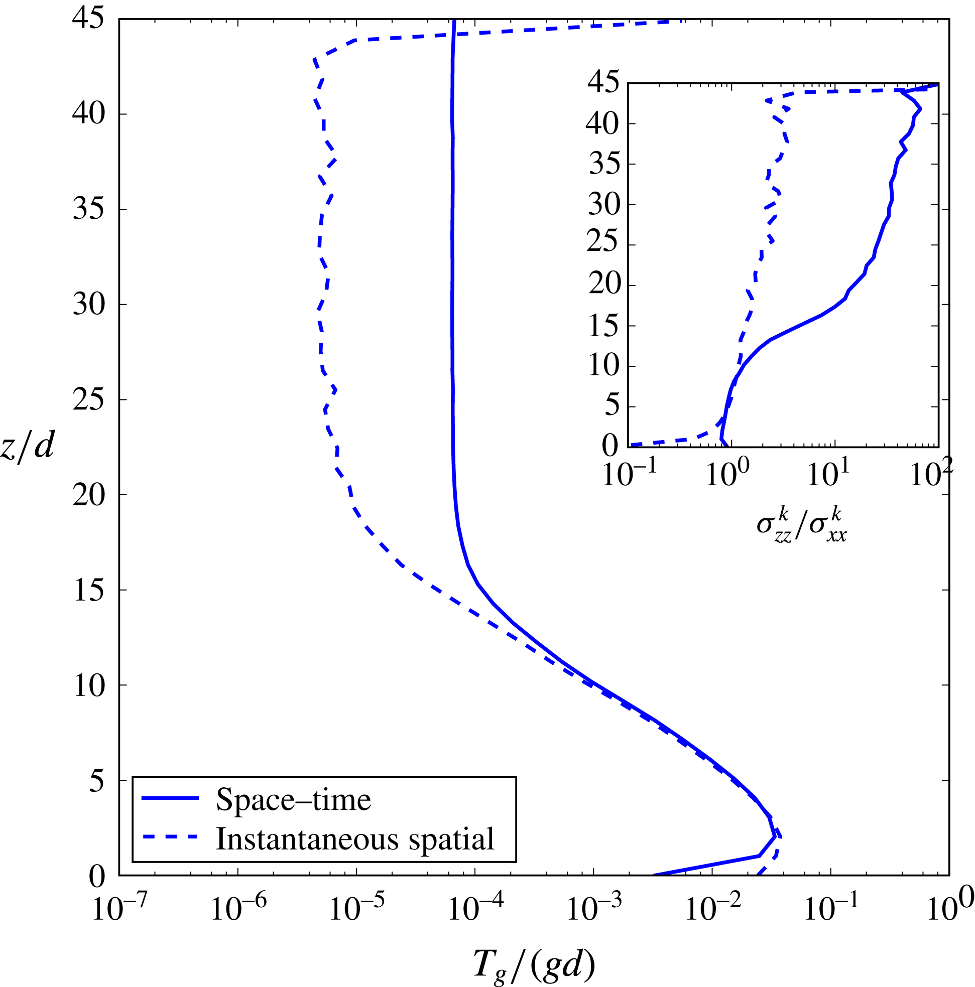
. Fluctuations are defined with respect to space–time averaged velocity profile (solid lines) and to instantaneous spatial averages (dashed lines). The inset displays profiles of the ratio between vertical and horizontal normal kinetic stresses.

As concerns granular temperature profiles (displayed in figure 5
c), they are characterized by a first increase between
 $z=0$
and
 $z=(2{-}3)d$
, an exponential decay in the rest of the high-shear zone, and then a plateau in the creep zone. Particularly, granular temperature profiles for different values of the Froude number superpose when rescaled by
 $V^{1.5}$
, in the high-shear zone (not shown). It is evident that dimensional arguments would suggest
 $T\propto V^{2}$
; the same applies for standard kinetic theory when assuming negligible diffusive (i.e. non-local) effects. The difference between the observed velocity dependence of the granular temperature and such simple arguments may therefore be referred to non-local effects, but also to a peculiar behaviour of the cooperativity length of dissipation phenomena. This seems an interesting benchmark in the perspective of developing constitutive laws for dissipation and diffusion of fluctuating energy. The inset shows that vertical and horizontal velocity correlations are not equal, but vertical velocity correlations (translated by the kinetic stress component
 $\unicode[STIX]{x1D70E}_{zz}^{k}$
) are one order of magnitude higher than horizontal ones (
 $\unicode[STIX]{x1D70E}_{xx}^{k}$
) in the creep zone. In order to understand the origin of this difference in normal kinetic stresses, it is interesting to compare (figure 6) granular temperature and normal kinetic stress ratios computed with the different definitions of velocity fluctuations as discussed in § 3.2. It is evident that defining velocity fluctuations with respect to instantaneous averages yields lower values of the granular temperature in the creep zones, which proves that the creep zone is characterized by collective motions. The inset of figure 6 clearly shows that, for kinetic stresses based on instantaneous velocity averages, there is no normal stress difference; this proves that in collective motions an important role is played by vertical velocity fluctuations.
Effect of load (solid lines,
 $\tilde{M}=0.2$
; dashed lines,
 $\tilde{M}=2$
) and wall friction on kinematic profiles, for
 $Fr=1$
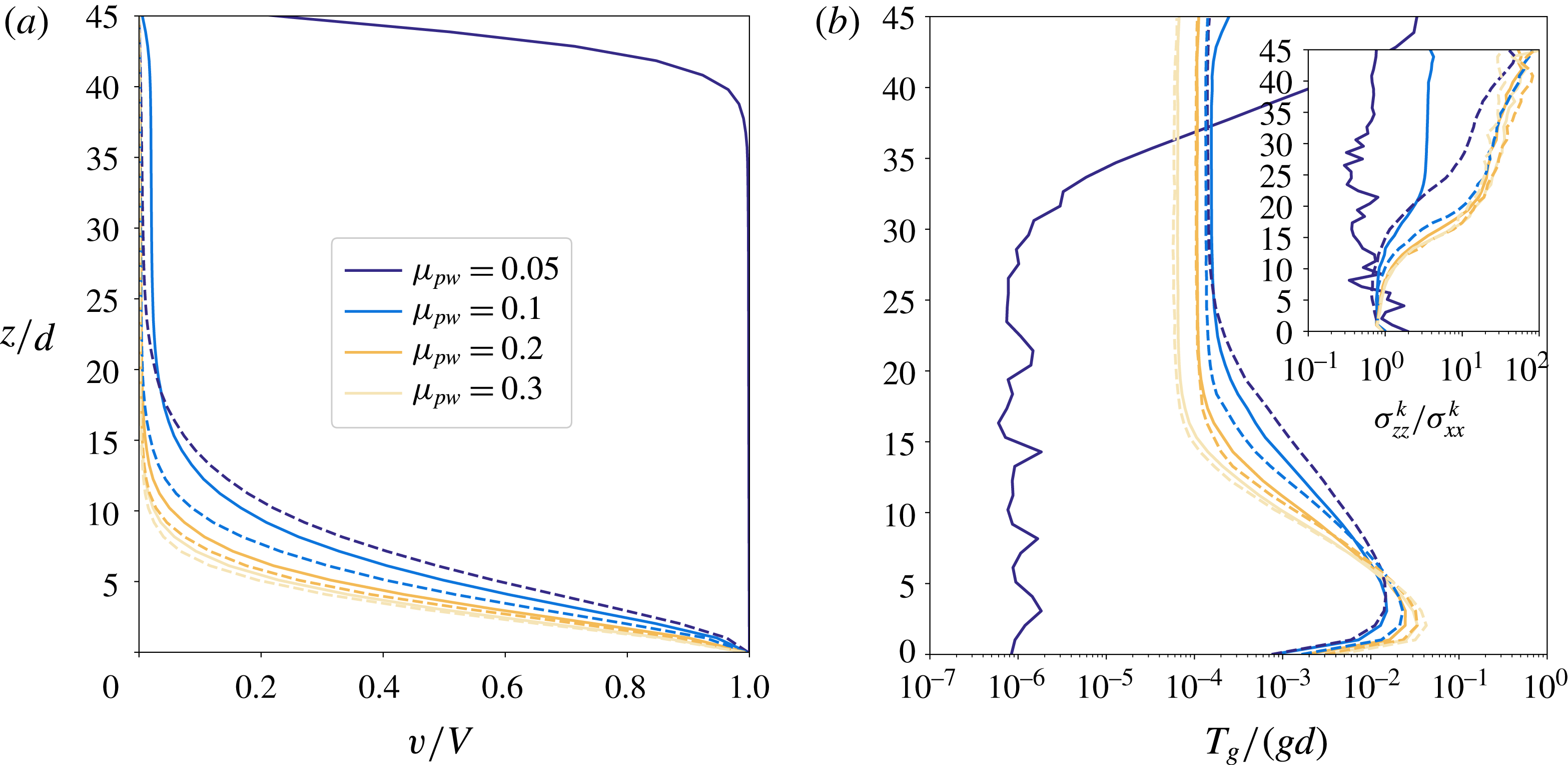
. (a) Velocity profiles characterized by different shear localization regimes. (b) Granular temperature profiles (inset: ratio between vertical and horizontal normal kinetic stresses).

The interest of numerical simulations is also to study the effect of parameters which are not easily varied in experiments. This is the case for the wall friction coefficient, and particularly in the low-friction limit. That is why we tested values corresponding to moderate to negligible wall friction conditions. The effect of wall friction on velocity profiles is displayed in figure 7(a) in conjunction with the externally applied load. It is interesting to observe that numerical simulations enrich the phenomenology observed in the experiments by the appearance of a new flow regime. For low friction and low applied load, the shear localization pattern is inverted with respect to high friction, and displays localization of the shear near the top wall instead of the bottom one. Opposite to the moderate friction case, in this situation the top shear zone is accompanied by a plug flow region where the grains move nearly as a solid block with the bottom wall. If the load is increased, the profile may switch to a bottom localized one. For bottom localization, the decay length of the exponential decreases when increasing wall friction or load, and the profiles suggest an asymptotic behaviour for the decay length as in the experiments. For low load and intermediate friction (e.g. the curve corresponding to
 $\tilde{M}=0.2$
and
 $\unicode[STIX]{x1D707}_{pw}=0.1$
in figure 7
a), instead of the creep zone, a plug flow zone moving at low velocity develops, and shear increases again near the top wall. Such shear localization patterns were already pointed out in Artoni & Richard (Reference Artoni and Richard2015b
), and referred to as: (A) bottom localization with creep zone at the top; (B) plug flow at the bottom with shear localization near the top wall; and (C) bottom localization with a slow plug flow instead of the creep zone. Note that in regime C, the shear zone at the top is very small (
 $(1{-}2)d$
) and can probably be seen as an apparent slip between the particles and the top wall. As concerns granular temperature, figure 7(b) shows that when load and/or wall friction is increased, the plateau is at lower values of
 $T_{g}$
and is attained at lower
 $z$
. For low load and low wall friction (regime B), the temperature profile is inverted and fluctuating energy is very low in the plug region. Also, the inset shows that in regimes B and C vertical velocity fluctuations are relatively less important than in regime A.
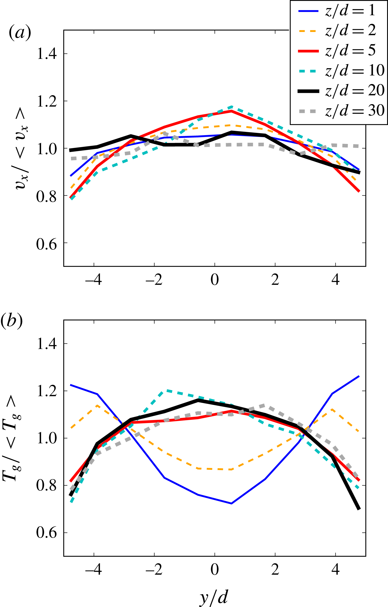
The transverse relative variations of the velocity (a) and of the granular temperature (b) are small. Depending on the flow regime (sheared or quasi-static), the sidewalls behave like a source or a sink of granular temperature.

Figure 8 depicts the transverse velocity (a) and temperature (b) profiles in the case
 $\unicode[STIX]{x1D707}_{pw}=0.3$
and
 $\tilde{M}=0.2$
for several vertical positions within the flow. With this set of parameters, shear is localized at the bottom of the simulation cell. The corresponding vertical profiles have been reported in figure 7. The transverse variations are small (
 $\pm 20\,\%$
) compared to the streamwise averages, justifying the
 $y$
averaging of our data mentioned at the beginning of this section. Interestingly, in the case of the velocity, the largest variations are found for the sheared zone (
 $z/d=1$
, 2, 5 and 10), those of the quasi-static zone being negligible. The temperature profile is very informative. In the zone corresponding to shear localization, this quantity is greatest at the sidewalls and lowest in the centre. In contrast, in the quasi-static zone, the granular temperature gradually rises from its minimal value at the sidewalls to a maximum value at the centre of the cell. Consequently, sidewalls could be either a granular heat source (in the sheared zone) or a sink (in the quasi-static zone) depending on the flow regimes. This points out the difficulty of stipulating a sidewall boundary condition on the granular temperature for theories aiming to capture the properties of granular flows in complex geometries. These results also demonstrate the importance of studying the interactions between granular media and interfaces.
Note also that further examination of the kinematics reveals the existence of secondary flows in the
 $y{-}z$
plane (not shown here) superimposed over the main flow. They are observed for low sidewall–grain friction coefficients (e.g.
 $\unicode[STIX]{x1D707}_{pw}=0.1$
) and are similar to those observed in the literature (Brodu et al.
Reference Brodu, Richard and Delannay2013, Reference Brodu, Delannay, Valance and Richard2015; Krishnaraj & Nott Reference Krishnaraj and Nott2016). Their velocity scale is small compared to that of the main flow and not easily measurable for higher sidewall–grain friction coefficients, probably because the width of our cell is small (
 $W=10d$
). These secondary flows are characterized by two counter-rotating convection rolls located in the sheared zone. Similarly to what has been observed in Brodu et al. (Reference Brodu, Richard and Delannay2013), the corresponding motion of the grains is upward along the sidewalls and downward in the middle of the simulation cell.
5.2 Stresses
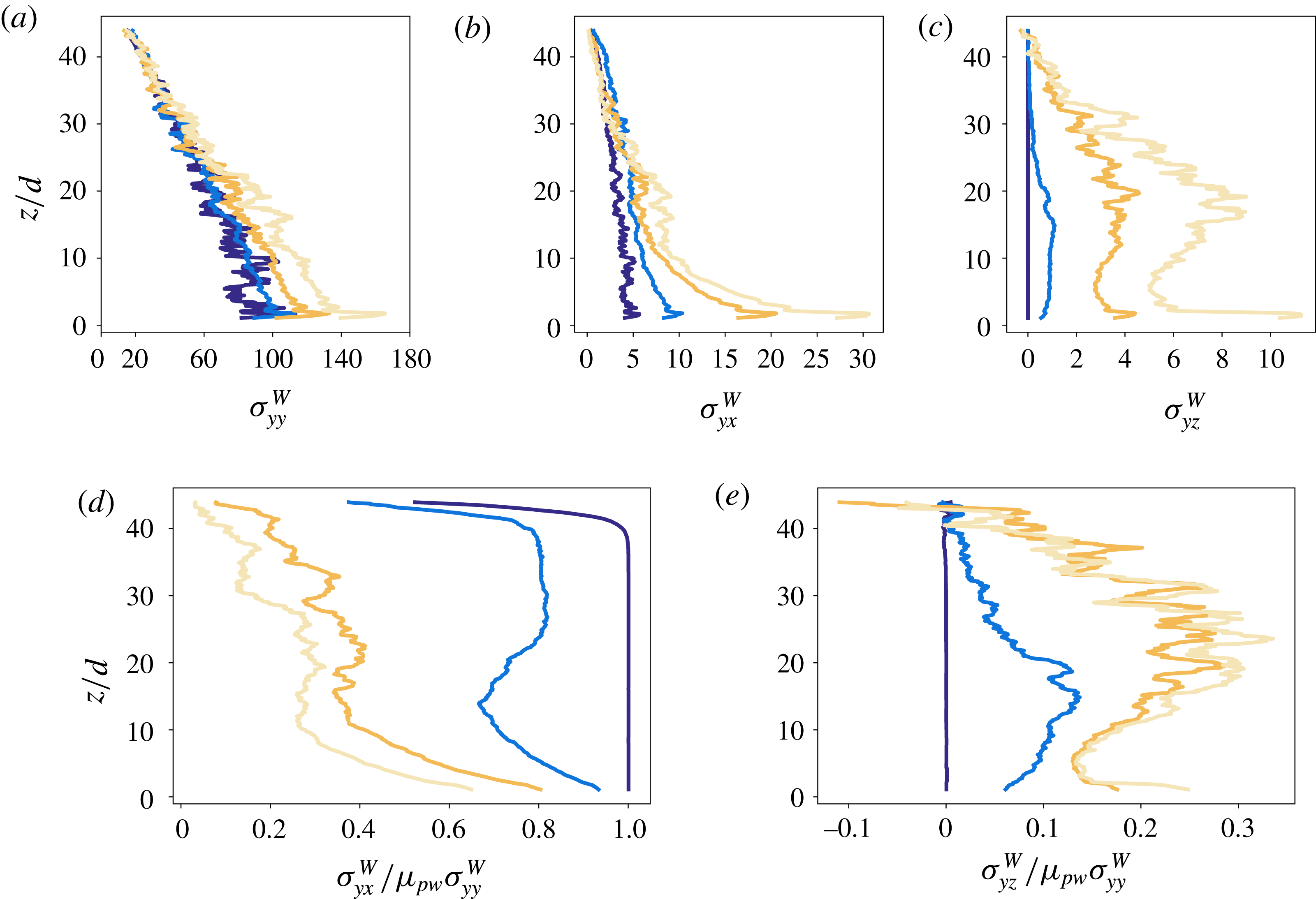
Wall stress profiles for
 $\tilde{M}=0.2$
,
 $Fr=1$
and different values of the particle–wall friction coefficient
 $\unicode[STIX]{x1D707}_{pw}$
: (a)
 $\unicode[STIX]{x1D70E}_{yy}^{W}$
; (b)
 $\unicode[STIX]{x1D70E}_{yx}^{W}$
; (c)
 $\unicode[STIX]{x1D70E}_{yz}^{W}$
; (d) effective, streamwise, wall friction coefficient
 $\unicode[STIX]{x1D70E}_{yx}^{W}/\unicode[STIX]{x1D70E}_{yy}^{W}$
rescaled by
 $\unicode[STIX]{x1D707}_{pw}$
; and (e) effective, transverse, wall friction coefficient
 $\unicode[STIX]{x1D70E}_{yz}^{W}/\unicode[STIX]{x1D70E}_{yy}^{W}$
rescaled by
 $\unicode[STIX]{x1D707}_{pw}$
.

In the experiments, wall stresses were measured at three vertical positions. Numerical simulations allow one to extract full wall stress profiles in
 $z$
. As an example, figure 9(a–c) displays profiles of relevant wall stresses (
 $\unicode[STIX]{x1D70E}_{yy}^{W},~\unicode[STIX]{x1D70E}_{yx}^{W},~\unicode[STIX]{x1D70E}_{yz}^{W}$
) for
 $\tilde{M}=0.2$
,
 $Fr=1$
and different values of the particle–wall friction coefficient
 $\unicode[STIX]{x1D707}_{pw}$
. When comparing qualitatively the numerical results to the experiments described above, one has to consider that all the experimental flows reported in § 4, in view of the velocity profiles and the force values measured, appear to belong to regime A of shear localization, which means that wall friction is relatively strong. First, wall-normal stress (figure 9
a) appears nearly hydrostatic and quite independent of flow rate (not shown here). Wall friction has a slight but well-defined effect on
 $\unicode[STIX]{x1D70E}_{yy}^{W}$
: the normal stress increases with
 $\unicode[STIX]{x1D707}_{pw}$
in the lower part of the cell, yielding a moderate deviation from the hydrostatic profile for high friction. This deviation can be ascribed to the presence of stress component
 $\unicode[STIX]{x1D70E}_{yz}^{W}$
, which increases with
 $\unicode[STIX]{x1D707}_{pw}$
(see appendix A). Numerical wall-normal stresses are therefore in excellent agreement with experimental observations. Apart from normal stresses, it is evident that
 $\unicode[STIX]{x1D707}_{pw}$
has a clear effect on wall tangential stresses, as both
 $\unicode[STIX]{x1D70E}_{yx}^{W}$
and
 $\unicode[STIX]{x1D70E}_{yz}^{W}$
increase with
 $\unicode[STIX]{x1D707}_{pw}$
. While
 $\unicode[STIX]{x1D70E}_{yx}^{W}$
(figure 9
b) decreases almost monotonically with
 $z$
,
 $\unicode[STIX]{x1D70E}_{yz}^{W}$
(figure 9
c) may display a first increase, a plateau and a decrease near the top (particularly for high friction). The balance between
 $\unicode[STIX]{x1D70E}_{yx}^{W}$
and
 $\unicode[STIX]{x1D70E}_{yz}^{W}$
depends on wall friction and
 $z$
. For high wall friction (regime A),
 $\unicode[STIX]{x1D70E}_{yx}^{W}>\unicode[STIX]{x1D70E}_{yz}^{W}$
in the lower portion of the cell, and
 $\unicode[STIX]{x1D70E}_{yx}^{W}\sim \unicode[STIX]{x1D70E}_{yz}^{W}$
in the creep zone. In regimes B and C we always observe
 $\unicode[STIX]{x1D70E}_{yx}^{W}\gg \unicode[STIX]{x1D70E}_{yz}^{W}$
given that wall friction is nearly everywhere mobilized in the
 $x$
direction. It is also important to note that for some parameter values (e.g. high
 $\tilde{M}$
),
 $\unicode[STIX]{x1D70E}_{yz}^{W}$
may change its sign from the shear zone where
 $\unicode[STIX]{x1D70E}_{yz}^{W}>0$
to the vicinity of the top wall where
 $\unicode[STIX]{x1D70E}_{yz}^{W}<0$
, exactly as observed in some experiments. As discussed in appendix A,
 $\unicode[STIX]{x1D70E}_{yz}^{W}>0$
may come from an upward motion of grains near the wall (which is the case in the sheared zone as described in the previous section), but also from the coupling between the flow dynamics and the non-smooth nature of wall friction (in relation to collective motions in the creep zone). In order to study effective wall friction, in figure 9(d,e) we look at profiles of the rescaled effective friction coefficients
 $\unicode[STIX]{x1D70E}_{yx}^{W}/\unicode[STIX]{x1D707}_{pw}\unicode[STIX]{x1D70E}_{yy}^{W}$
and
 $\unicode[STIX]{x1D70E}_{yz}^{W}/\unicode[STIX]{x1D707}_{pw}\unicode[STIX]{x1D70E}_{yy}^{W}$
.
It is evident that these effective coefficients critically depend on the flow regime. For regime B,
 $\unicode[STIX]{x1D70E}_{yx}^{W}/\unicode[STIX]{x1D707}_{pw}\unicode[STIX]{x1D70E}_{yy}^{W}\approx 1$
and
 $\unicode[STIX]{x1D70E}_{yz}^{W}/\unicode[STIX]{x1D707}_{pw}\unicode[STIX]{x1D70E}_{yy}^{W}\approx 0$
, while, when increasing
 $\unicode[STIX]{x1D707}_{pw}$
,
 $\unicode[STIX]{x1D70E}_{yx}^{W}/\unicode[STIX]{x1D707}_{pw}\unicode[STIX]{x1D70E}_{yy}^{W}$
decreases and
 $\unicode[STIX]{x1D70E}_{yz}^{W}/\unicode[STIX]{x1D707}_{pw}\unicode[STIX]{x1D70E}_{yy}^{W}$
increases, which is a signature of both friction weakening related to stick–slip motions (Richard et al.
Reference Richard, Valance, Métayer, Sanchez, Crassous, Louge and Delannay2008; Artoni, Santomaso & Canu Reference Artoni, Santomaso and Canu2009; Artoni et al.
Reference Artoni, Santomaso, Go and Canu2012; Artoni & Richard Reference Artoni and Richard2015b
) and of force orientation dispersion increasing the importance of vertical components.
6 Discussion
Both experiments and simulations were characterized by interesting shear localization features, accompanied by a peculiar friction weakening behaviour. In the following, we employ a simplified stress analysis to propose an explanation of the velocity profiles obtained. Flowing granular materials can be described as a peculiar class of viscoplastic fluids, in which the yield stress is proportional to pressure. There may be debate about the details of such a picture, for example about the real existence of a yield stress, the type of yield criterion, non-local effects diffusing shear to subcritical zones, and so on. Without entering into such details, the frictional character of granular materials remains quite evident, and implies that under controlled stress conditions the amount of shear is a function of the ratio between shear and normal stress
 $\unicode[STIX]{x1D70F}/p$
instead of
 $\unicode[STIX]{x1D70F}$
. This means that a heterogeneity in effective bulk friction is likely to produce heterogeneity in shear, which can be characterized by shear localization if part of the material is in subcritical conditions (see appendix A). When this is considered, we can see that three situations appear (we focus on the geometry used in the simulations and therefore use Cartesian coordinates).
Case A. Strong wall friction, independently of pressure:
 $\unicode[STIX]{x1D70E}_{zx}/\unicode[STIX]{x1D70E}_{zz}$
may decrease with
 $z$
, so shear is higher (localized) at the bottom of the cell.
Case B. Negligible wall friction, low applied pressure:
 $\unicode[STIX]{x1D70E}_{zx}/\unicode[STIX]{x1D70E}_{zz}$
increases with
 $z$
, so shear is higher (localized) at the top of the cell.
Case C. Negligible wall friction, high applied pressure:
 $\unicode[STIX]{x1D70E}_{zx}/\unicode[STIX]{x1D70E}_{zz}$
may be uniform in
 $z$
, and shear may be quite uniform as well.
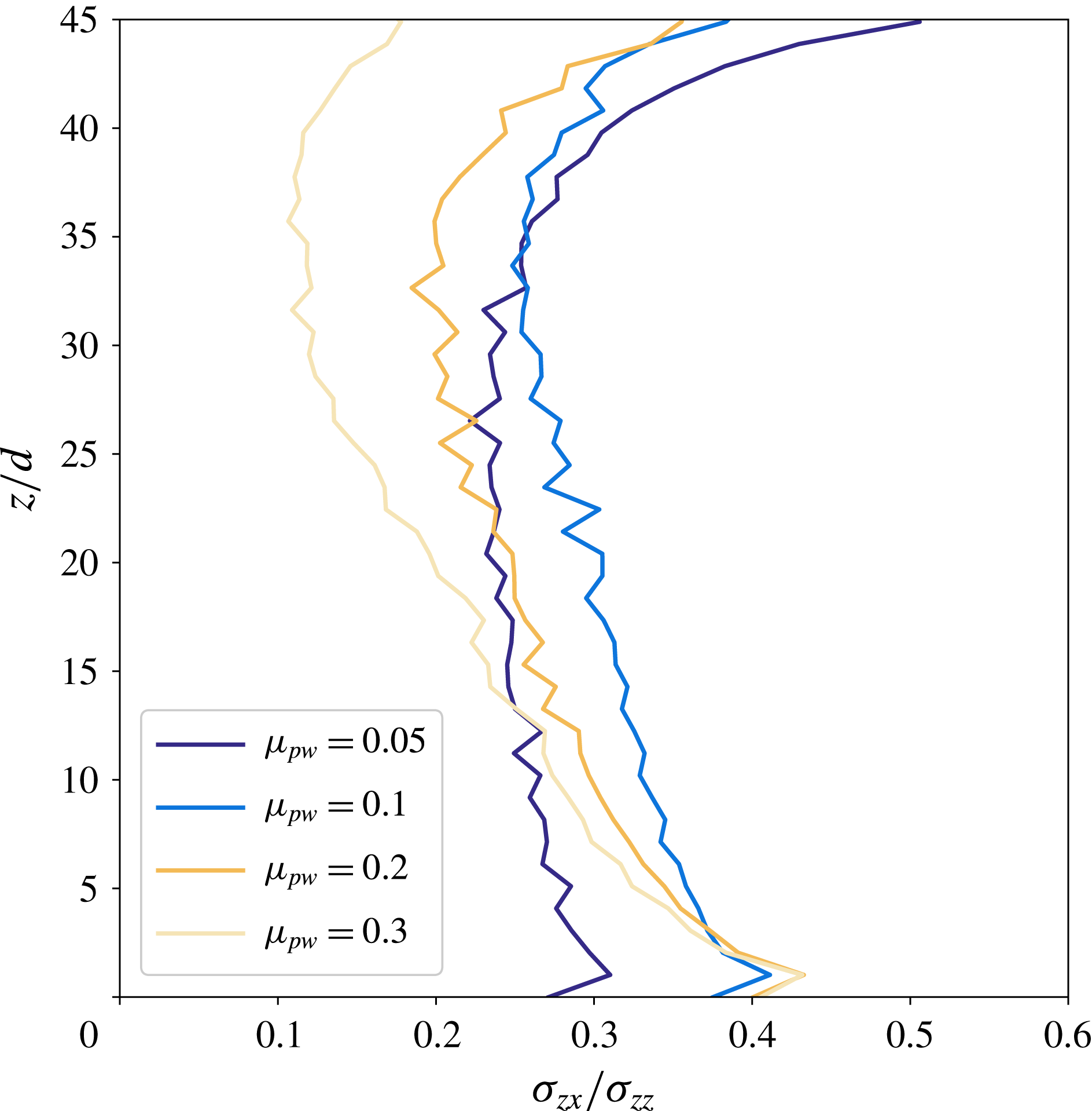
The results of this simplified analysis are confirmed by numerical results: for strong wall friction, numerical profiles along
 $z$
of the ratio
 $\unicode[STIX]{x1D70E}_{zx}/\unicode[STIX]{x1D70E}_{zz}$
, which are displayed in figure 10, decrease clearly with
 $z$
. When decreasing
 $\unicode[STIX]{x1D707}_{pw}$
, the slope of the
 $\unicode[STIX]{x1D70E}_{zx}/\unicode[STIX]{x1D70E}_{zz}$
versus
 $z$
profile decreases accordingly. For the lower value of
 $\unicode[STIX]{x1D707}_{pw}$
(which corresponds to regime B), the value of the stress ratio is nearly uniform and lower than the other cases in the lower region, and displays a strong increase with
 $z$
in the top region. The non-monotonic nature of the stress ratio profile clearly shows that the picture is more complex than the one drawn in the simplified analysis developed above, but the heart of the phenomenology is captured.
Profiles along
 $z$
of the bulk stress ratio
 $\unicode[STIX]{x1D70E}_{zx}/\unicode[STIX]{x1D70E}_{zz}$
(with the bulk stress components averaged in the
 $y$
direction) for
 $\tilde{M}=0.2$
,
 $Fr=1$
and different values of the particle–wall friction coefficient
 $\unicode[STIX]{x1D707}_{pw}$
.

Therefore, the shear localization patterns which were observed in experiments and numerical simulations are explained by the effective bulk friction heterogeneity, which is due to the interplay of gravity and sidewall friction. The simplified stress analysis discussed here provides a basis for understanding the effect of applied load, wall friction and aspect ratio of the cell. A strong conclusion from the present section is that a detailed rheology is not needed to predict the effect of these parameters. However, in order to understand the rate independence of rescaled velocity profiles, the present analysis is not enough, since rheology is not included in the discussion. The use of
 $\unicode[STIX]{x1D707}(I)$
rheology, even under an energy dissipation perspective, would predict large variation of the decay of the velocity profile with the velocity of the bottom wall (Artoni & Richard Reference Artoni and Richard2018). It is probable that including non-locality by a diffusing order parameter would solve this problem. This will be the subject of a detailed future analysis.
7 Conclusions
Our work sheds light on the complexity of confined flows which may display complex shear localization patterns. In this paper, we indeed investigated dry granular flows in a shear cell by combining experiments and discrete element method (DEM) numerical simulations and focus on the stress heterogeneity induced by sidewalls, which yields, in turn, shear heterogeneity. The shear cell used in this work is annular with a bumpy bottom which rotates at constant velocity and a bumpy top on which a pressure is applied. The inner and outer cylinders of the cell are flat but frictional. Experimentally, by means of PIV, we have shown that the depth velocity profiles are exponential functions characterized by a decay length depending on the applied stress but independent of the shearing velocity. Our force measurements report force weakening at the sidewalls, a phenomenon which was already observed numerically in confined chute flows (Richard et al. Reference Richard, Valance, Métayer, Sanchez, Crassous, Louge and Delannay2008) and, more recently, in a torsional shear cell (Artoni & Richard Reference Artoni and Richard2018). To enhance our analysis, we have carried out DEM simulations that have shown that, depending on the sidewall friction, the shear can be localized at the bottom of the cell, close to its top or more or less uniformly along the depth of the cell. We have derived a theoretical stress analysis for which we assumed the system to be a continuous medium. It shows that the aforementioned shear localization is explained by the effective bulk friction heterogeneity. It also links the three observed regimes to two parameters: the applied pressure and the sidewall friction. The first regime corresponds to important sidewall friction (shear localized at the bottom); in the second one, sidewall friction is negligible and the applied pressure is low (localization of the shear close to top); the third case, corresponding to negligible sidewall friction and important applied pressure, leads to an almost uniform shear.
To go further in the understanding of these complex flows, a full three-dimensional rheological description of a granular flow is probably required. Yet, the studied geometry, by the complexity of the flow it produces and by the importance of its interfaces, is well adapted for testing granular rheologies numerically and studying boundary conditions. In particular, the presence of interfaces highlights the importance of non-local effects on flow behaviour (Kamrin & Koval Reference Kamrin and Koval2012; Bouzid et al. Reference Bouzid, Trulsson, Claudin, Clément and Andreotti2013, Reference Bouzid, Trulsson, Claudin, Clément and Andreotti2015; Kamrin & Henann Reference Kamrin and Henann2015; Nott Reference Nott2017; Zhang & Kamrin Reference Zhang and Kamrin2017); our system is thus a relevant system to test the theories taking into account the latter effects.
Acknowledgement
The numerical simulations were carried out at the CCIPL (Centre de Calcul Intensif des Pays de la Loire) under the project MTEEGD.
Appendix A. Simplified stress analysis
For the sake of simplicity, we focus on the geometry used in the simulations and therefore use Cartesian coordinates. Stress balances (sign convention of positive compressive stresses is used throughout this paper) can be simplified by considering periodicity of the flow (
 $\unicode[STIX]{x2202}/\unicode[STIX]{x2202}x=0$
):
 $$\begin{eqnarray}\left.\begin{array}{@{}c@{}}\unicode[STIX]{x2202}_{y}\unicode[STIX]{x1D70E}_{yx}+\unicode[STIX]{x2202}_{z}\unicode[STIX]{x1D70E}_{zx}=0,\\ \unicode[STIX]{x2202}_{y}\unicode[STIX]{x1D70E}_{yy}+\unicode[STIX]{x2202}_{z}\unicode[STIX]{x1D70E}_{zy}=0,\\ \unicode[STIX]{x2202}_{y}\unicode[STIX]{x1D70E}_{yz}+\unicode[STIX]{x2202}_{z}\unicode[STIX]{x1D70E}_{zz}=-\unicode[STIX]{x1D70C}g.\end{array}\right\}\end{eqnarray}$$
Wall friction yields forces on the wall plane, which means that stress components
 $\unicode[STIX]{x1D70E}_{yy}^{W}$
,
 $\unicode[STIX]{x1D70E}_{yx}^{W}$
,
 $\unicode[STIX]{x1D70E}_{yz}^{W}\neq 0$
at the wall.
Let us consider now the case in which lateral wall friction is no longer negligible. To simplify the discussion, together with the assumption of no normal stress difference, we assume linearity of
 $\unicode[STIX]{x1D70E}_{yx}$
and
 $\unicode[STIX]{x1D70E}_{yz}$
in
 $y$
(and symmetry of the stress tensor). In other words,
 $$\begin{eqnarray}\unicode[STIX]{x1D70E}_{yx}=\unicode[STIX]{x1D70E}_{xy}=\unicode[STIX]{x1D70E}_{yx}^{W}\frac{2y}{W},\quad \unicode[STIX]{x1D70E}_{yz}=\unicode[STIX]{x1D70E}_{zy}=\unicode[STIX]{x1D70E}_{yz}^{W}\frac{2y}{W}.\end{eqnarray}$$
Let us recall here that the
 $y=0$
plane is located at mid-distance between the two sidewalls (figure 2). Stress balances in (A 1) therefore yield
 $$\begin{eqnarray}\left.\begin{array}{@{}c@{}}\displaystyle \frac{2}{W}\unicode[STIX]{x1D70E}_{yx}^{W}+\unicode[STIX]{x2202}_{z}\unicode[STIX]{x1D70E}_{zx}=0,\\ \displaystyle \unicode[STIX]{x2202}_{y}\unicode[STIX]{x1D70E}_{yy}+\frac{2y}{W}\unicode[STIX]{x2202}_{z}\unicode[STIX]{x1D70E}_{yz}^{W}=0,\\ \displaystyle \frac{2}{W}\unicode[STIX]{x1D70E}_{yz}^{W}+\unicode[STIX]{x2202}_{z}\unicode[STIX]{x1D70E}_{zz}=-\unicode[STIX]{x1D70C}g.\end{array}\right\}\end{eqnarray}$$
From this system of equations it is clear that
 $\unicode[STIX]{x1D70E}_{yz}^{W}$
affects normal stress profiles, and that
 $\unicode[STIX]{x1D70E}_{yx}^{W}$
influences the main shear stress,
 $\unicode[STIX]{x1D70E}_{zx}$
. Considering the sign convention used for stress, and given that the force exerted by sidewalls in the
 $x$
direction is opposite to the flow direction, it is evident that
 $\unicode[STIX]{x1D70E}_{yx}^{W}>0$
. Assuming that
 $\unicode[STIX]{x1D70E}_{yx}^{W}$
scales on pressure through a scaling
 $\unicode[STIX]{x1D70E}_{yx}^{W}=\unicode[STIX]{x1D707}_{x}^{W}\unicode[STIX]{x1D70E}_{yy}^{W}$
, two things are evident:
(i)
 $\unicode[STIX]{x1D70E}_{zx}$
decreases with
$z$
due to wall friction;
(ii)
$\unicode[STIX]{x1D707}_{x}^{W}$
cannot be constant, otherwise
$\unicode[STIX]{x1D70E}_{zx}$
could become negative (Richard et al.
Reference Richard, Valance, Métayer, Sanchez, Crassous, Louge and Delannay2008).


While the sign of
 $\unicode[STIX]{x1D70E}_{yx}^{W}$
is dictated by the flow direction, the issue is more puzzling for
 $\unicode[STIX]{x1D70E}_{yz}^{W}$
. In statics it is natural to think that walls partially support the weight of the granular material, and that therefore forces at the wall are upward-oriented, which means that
 $\unicode[STIX]{x1D70E}_{yz}^{W}<0$
. However, with the granular material flowing in the
 $x$
direction, it is not evident whether this relation holds or not. For example, a secondary flow inducing upward motion of particles in contact with the wall induces
 $\unicode[STIX]{x1D70E}_{yz}^{W}>0$
. But also collective vertical motions in the creep zones, coupled with asymmetric force fluctuations may, due to the non-smooth nature of friction, contribute to a positive
 $\unicode[STIX]{x1D70E}_{yz}^{W}$
.
In order to obtain a simplified evaluation of the effect of wall friction on bulk friction heterogeneity, let us assume that
 $\unicode[STIX]{x1D70E}_{yz}^{W}=0$
, and that
 $\unicode[STIX]{x1D707}_{x}^{W}$
is constant. This implies that the profile of
 $\unicode[STIX]{x1D70E}_{zz}$
is the same as in the negligible wall friction case. A possible measure for bulk friction heterogeneity is the difference
 $\unicode[STIX]{x1D70E}_{zx}/\unicode[STIX]{x1D70E}_{zz}$
from the top to the bottom, which is therefore
 $$\begin{eqnarray}\unicode[STIX]{x0394}\left(\frac{\unicode[STIX]{x1D70E}_{zx}}{\unicode[STIX]{x1D70E}_{zz}}\right)=\frac{\unicode[STIX]{x1D70E}_{zx}(0)}{\unicode[STIX]{x1D70E}_{zz}(H)+\unicode[STIX]{x1D70C}gH}\frac{\unicode[STIX]{x1D70C}gH}{\unicode[STIX]{x1D70E}_{zz}(H)}-2\unicode[STIX]{x1D707}_{x}^{W}K\frac{H}{W}\left(1+\frac{\unicode[STIX]{x1D70C}gH}{2\unicode[STIX]{x1D70E}_{zz}(H)}\right),\end{eqnarray}$$
where
 $\unicode[STIX]{x1D70E}_{zx}(0)$
is the value of the shear stress at the bottom boundary,
 $\unicode[STIX]{x1D70E}_{zz}(H)$
is the external stress induced by the force at the top plate and
 $K=\unicode[STIX]{x1D70E}_{yy}/\unicode[STIX]{x1D70E}_{zz}$
is a coefficient measuring the balance between horizontal and vertical normal stresses (similar to Rankine’s coefficient of lateral earth pressure). In the case of frictionless sidewalls (
 $\unicode[STIX]{x1D707}_{x}^{W}=0$
) the quantity
 $\unicode[STIX]{x0394}(\unicode[STIX]{x1D70E}_{zx}/\unicode[STIX]{x1D70E}_{zz})$
is strictly positive and decreases with
 $\unicode[STIX]{x1D70E}_{zz}(H)$
tending asymptotically to 0. On the contrary, the introduction of (sufficiently strong) wall friction opens the possibility of
 $\unicode[STIX]{x0394}(\unicode[STIX]{x1D70E}_{zx}/\unicode[STIX]{x1D70E}_{zz})<0$
. Equation (A 4) also suggests that the aspect ratio
 $H/W$
enhances the effect of wall friction, and that the effect of pressure is not the same as for negligible wall friction. It is evident that if
 $\unicode[STIX]{x1D70E}_{zz}(H)\rightarrow \infty$
, then
 $\unicode[STIX]{x0394}(\unicode[STIX]{x1D70E}_{zx}/\unicode[STIX]{x1D70E}_{zz})\rightarrow -\unicode[STIX]{x1D707}_{x}^{W}H/W$
. This result highlights the fact that the increase of pressure does not remove bulk friction heterogeneity, but enforces the decrease of
 $\unicode[STIX]{x1D70E}_{zx}/\unicode[STIX]{x1D70E}_{zz}$
with
 $z$
.