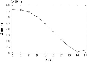
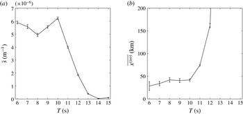
1. Introduction
There is now growing evidence that ocean surface waves have a significant impact on the seasonal advance and retreat of sea ice in the Arctic and Southern Oceans. Satellite observations have shown that the energy content of wave spectra in the polar oceans has been trending upwards in the last three decades, more significantly than at lower latitudes (Young, Zieger & Babanin Reference Young, Zieger and Babanin2011). Recent in situ observations and hindcasts of energetic wave fields at high latitudes (Kohout et al.
Reference Kohout, Williams, Dean and Meylan2014; Thomson & Rogers Reference Thomson and Rogers2014; Collins et al.
Reference Collins, Rogers, Marchenko and Babanin2015) support these long-term trends and suggest an increasing impact of waves on the morphology of ice-covered oceans. In particular, waves contribute to the rapid decline of sea ice extent and thickness observed in the Arctic region (Laxon et al.
Reference Laxon, Giles, Ridout, Wingham, Willatt, Cullen, Kwok, Schweiger, Zhang and Haas2013; Meier, Gallaher & Campbell Reference Meier, Gallaher and Campbell2013) by fracturing the elastic ice cover under sufficient flexural load (see Squire et al.
Reference Squire, Dugan, Wadhams, Rottier and Liu1995; Squire Reference Squire2007, for reviews), and therefore accelerating the melting of sea ice. This contribution is most pronounced within, say, 100 km of the ice edge, a region referred to as the marginal ice zone (MIZ), which typically consists of a disordered array of floating ice floes with various shapes and characteristic horizontal dimensions
 $O(10{-}100~\text{m})$
.
The presence of a broken-up ice cover with a certain ice concentration (the fraction of sea surface covered by ice), thickness and floe size distribution (FSD) governs the evolution of wave spectral properties (energy content, frequency and direction) within the MIZ. When ocean waves enter an MIZ they are attenuated and, for modest seas, much evidence now supports the assertion that ocean wave energy decays at an exponential rate with distance from the ice edge (see Squire & Moore Reference Squire and Moore1980; Wadhams et al. Reference Wadhams, Squire, Goodman, Cowan and Moore1988; Meylan, Bennetts & Kohout Reference Meylan, Bennetts and Kohout2014, for field measurements in both the Arctic and Southern Oceans). Moreover, the rate of attenuation tends to increase with decreasing wave period. Concomitantly, the range of directions over which waves travel in the MIZ appears to increase with distance from the ice edge, so that the wave spectrum tends to become fully isotropic. Directional spreading in the MIZ has been observed during the field work of Wadhams et al. (Reference Wadhams, Squire, Ewing and Pascal1986) and has also been inferred from synthetic aperture radar imagery (see, e.g., Liu, Vachon & Peng Reference Liu, Vachon and Peng1991b ). Both wave energy attenuation and directional spreading are governed by a combination of scattering effects and dissipative processes. Wave energy dissipation occurs in many different forms, e.g. collisions (Shen & Squire Reference Shen and Squire1998; Bennetts & Williams Reference Bennetts and Williams2015), turbulence (Liu & Mollo-Christensen Reference Liu and Mollo-Christensen1988), wave overwash (Bennetts et al. Reference Bennetts, Alberello, Meylan, Cavaliere, Babanin and Toffoli2015; Skene et al. Reference Skene, Bennetts, Meylan and Toffoli2015), floe breakup (Williams et al. Reference Williams, Bennetts, Squire, Dumont and Bertino2013a ) and inelastic bending (Squire & Fox Reference Squire and Fox1992). Estimation of their effects on wave energy attenuation is a difficult task, as most are nonlinear processes. Although simplified empirical parameterizations have been developed to model the MIZ as a homogeneous linearly viscoelastic layer (Wang & Shen Reference Wang and Shen2010), their validity is unresolved and calibration presents a major challenge that requires more data than are currently available (Mosig, Montiel & Squire Reference Mosig, Montiel and Squire2015). In contrast, wave scattering is conservative and redistributes the wave energy over the directional domain. The exponential attenuation of wave energy and directional spreading is a direct consequence of linear multiple scattering theory for waves propagating in random media. This effect has been observed and modelled in many areas concerned with such processes (see, e.g., Ishimaru Reference Ishimaru1978).
Herein, a three-dimensional model of wave energy attenuation and directional spreading in the MIZ is proposed. Our goal is to reproduce the observed wave attenuation and directional spreading of ocean wave spectra as they propagate through the MIZ, by modelling the random nature of open ocean sea states and the disorder of the distribution of ice floes in the MIZ. The primary outcome will be an improved parameterization of wave/sea ice interactions in ice/ocean models (IOMs), e.g. TOPAZ, and spectral wave models (SWMs) such as Wavewatch III® or WAM. We plan to use our model simulations to generate attenuation and directional spreading parameters in the form of look-up tables. We note that at present only two-dimensional approaches (i.e. ones with one wave direction) are employed to model wave energy attenuation in such large-scale models, with no exchange of energy between different wave directions (see Doble & Bidlot Reference Doble and Bidlot2013; Rogers & Orzech Reference Rogers and Orzech2013; Williams et al. Reference Williams, Bennetts, Squire, Dumont and Bertino2013a ,Reference Williams, Bennetts, Squire, Dumont and Bertino b , for implementation in SWMs and IOMs).
Unidirectional wave energy attenuation in the MIZ, i.e. neglecting directional spreading, due to multiple scattering by arrays of ice floes has been described theoretically a number of times within the framework of linear potential flow theory (see Squire et al. Reference Squire, Dugan, Wadhams, Rottier and Liu1995; Squire Reference Squire2011, for reviews). The most common representation of each floe is a thin elastic plate. For example, Kohout & Meylan (Reference Kohout and Meylan2008) considered transmission of waves through multiple elastic plates floating with no submergence, using a two-dimensional model with one vertical dimension and one horizontal dimension. They used ensemble averaging to show that selecting floe lengths and floe spacings randomly from Rayleigh distributions leads to exponential attenuation of the proportion of mean wave energy transmitted with respect to the number of floes, and that the effective rate of attenuation increases with decreasing wave period. These behaviours mirror those of ocean waves in the MIZ. Kohout & Meylan further showed that their scattering model predicts attenuation rates comparable to those measured in the MIZ for midrange wave periods (approximately 6–15 s), but that it underpredicts the attenuation rates of longer period waves by at least an order of magnitude. Bennetts & Squire (Reference Bennetts and Squire2012b ) derived a semianalytic expression for the rate of exponential attenuation predicted by the two-dimensional model based upon the reflection produced by a solitary floe, assuming that the wave phase between floes is random, as opposed to varying the floe lengths and spacings. They also included a parameterization of wave energy dissipation due to interaction with the floes via the viscoelastic plate model of Robinson & Palmer (Reference Robinson and Palmer1990) to correct for attenuation of long-period waves. Bennetts & Squire (Reference Bennetts and Squire2012a ) subsequently went on to consider how sensitive the rate of exponential decay was to physical parameters in their model, with the direct purpose of intelligently assimilating wave–ice interactions in a contemporary IOM for the first time. Williams et al. (Reference Williams, Bennetts, Squire, Dumont and Bertino2013a ,Reference Williams, Bennetts, Squire, Dumont and Bertino b ) used the model of Bennetts & Squire (Reference Bennetts and Squire2012b ) to move towards this goal. Although these authors considered wavevectors from different directions, the scattering was inherently one-dimensional, with no changes to the directional structure of the wave spectrum being possible.
Several papers have outlined three-dimensional scattering models (two-dimensional waves) to predict attenuation through the MIZ. However, for the thousands of floes needed to simulate the MIZ, the computational expense of the additional dimension has led to the use of approximations and/or simplifications of the geometry. For example, Meylan, Squire & Fox (Reference Meylan, Squire and Fox1997) approximated the wave interactions between floes using the transport theory of radiative transfer in random media (based on the Boltzmann equation; see Ishimaru Reference Ishimaru1978), which does not resolve wave phases. They used the solitary circular elastic floe model of Meylan & Squire (Reference Meylan and Squire1996) to calculate the scattering kernel. They showed that, without an energy dissipation term, i.e. for scattering alone, wave energy attenuates for a finite distance only, after which it remains constant. Meylan & Masson (Reference Meylan and Masson2006) showed that the model of Meylan et al. (Reference Meylan, Squire and Fox1997) is almost identical to that of Masson & Leblond (Reference Masson and Leblond1989), who restricted their ice floe model to be a floating rigid cylinder. Bennetts et al. (Reference Bennetts, Peter, Squire and Meylan2010) proposed a model based on full potential flow theory, using the methods devised by Bennetts & Squire (Reference Bennetts and Squire2009) and Peter & Meylan (Reference Peter and Meylan2009). They considered square elastic floes in addition to circular floes, but found that the shape had minimal effect on predicted attenuation rates. They showed that the model gave excellent agreement with the measurements of Squire & Moore (Reference Squire and Moore1980) for midrange periods but, again, significantly underestimated the attenuation on long-period waves. Further, they studied the evolution of the directional spectrum of plane incident waves through the MIZ. However, for computational expediency, they imposed artificial periodic repetitions of a floe or groups of floes. This meant that the wave field was composed of plane waves travelling in a handful of different directions, where the exact number changed at certain wave periods. This led to artificial jumps in the attenuation rate with respect to the wave period, and no spreading of energy over the directional range was observed.
The three-dimensional model of wave attenuation and directional spreading in the MIZ proposed here is a solution of the full linear equations of potential flow theory and does not invoke artificial periodicity on the geometry. It extends the solution method proposed by Montiel, Squire & Bennetts (Reference Montiel, Squire and Bennetts2015a ) for a two-dimensional problem of acoustic wave propagation through a large finite array of identical circular obstructions. We include a realistic power-law FSD, which is based on the observational studies of Rothrock & Thorndike (Reference Rothrock and Thorndike1984), Toyota, Takatsuji & Nakayama (Reference Toyota, Takatsuji and Nakayama2006) and Toyota, Haas & Tamura (Reference Toyota, Haas and Tamura2011). Moreover, we model the incident wave forcing as a random sea state with a prescribed directional energy distribution. Ensemble averaging is then used to compute the wave energy attenuation and directional spreading through the MIZ.
2. Preliminaries
2.1. Governing equations
Consider a three-dimensional seawater domain with infinite horizontal extent and constant finite depth,
 $h$
say. Points in the water are located by Cartesian coordinates
 $(x,y)$
in the horizontal plane and
 $z$
in the vertical direction positively oriented upwards. We assume that the free surface at rest coincides with the plane
 $z=0$
, so the seabed is defined by
 $z=-h$
. Irregularities in the seabed are not considered here, as
 $h$
is assumed to be large compared with the wavelength throughout this study.
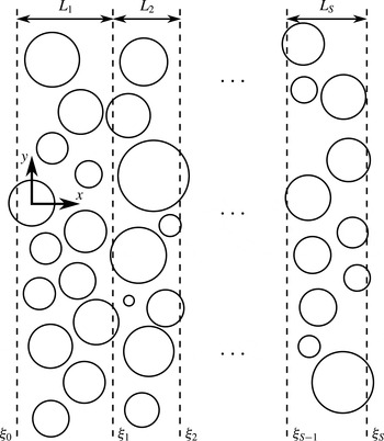
We seek to model the propagation of a directional ocean wave spectrum through an MIZ composed of thousands to tens of thousands of randomly positioned floating compliant ice floes with circular shape and uniform thickness. We only consider circular ice floes for simplicity, conjecturing that the shape of the floes has a small effect on the mean properties of wave propagation through large random arrays.
The solution method described in § 3 requires clustering of the array of floes into multiple slabs. Without loss of generality, we align the slabs with the
 $y$
-axis. Let
 $S$
denote the number of slabs, and let slab
 $q$
be bounded by
 ${\it\xi}_{q-1}\leqslant x\leqslant {\it\xi}_{q}$
,
 $1\leqslant q\leqslant S$
, have width
 $L_{q}={\it\xi}_{q}-{\it\xi}_{q-1}$
and contain
 $N_{q}$
floes. A sketch of the geometry is given in figure 1. It should be noted that a floe belongs to a slab if its centre is in the slab bounds.
Ice floe radii
 $a_{p}^{q}$
,
 $1\leqslant q\leqslant S$
,
 $1\leqslant p\leqslant N_{q}$
, are drawn from a prescribed power-law FSD as observed in the field (Toyota et al.
Reference Toyota, Takatsuji and Nakayama2006). A parameterization of the FSD will be described in § 5.2. Further, we assume that all floes have constant thickness
 $D$
and uniform density
 ${\it\rho}\approx 922.5~\text{kg}~\text{m}^{-3}$
. We do not include floes with different thicknesses and densities in the model in order to limit the number of parameters, although the method we propose can accommodate these extensions.
We consider a multidirectional wave field with small amplitude compared with the wavelength and prescribed angular frequency
 ${\it\omega}$
. The water is approximated as an inviscid and incompressible fluid with constant density
 ${\it\rho}_{0}\approx 1025~\text{kg}~\text{m}^{-3}$
and irrotational flow. The linear theory of water waves can then be used to describe the water motion. Assuming time-harmonic conditions, we express the velocity field in the water domain as
 $(\boldsymbol{{\rm\nabla}},\partial _{z})\text{Re}\{(g/\text{i}{\it\omega}){\it\phi}(x,y,z)\text{e}^{-\text{i}{\it\omega}t}\}$
, where
 $\boldsymbol{{\rm\nabla}}\equiv (\partial _{x},\partial _{y})$
and
 $g\approx 9.81~\text{m}~\text{s}^{-2}$
is the acceleration due to gravity. The complex-valued (reduced) potential,
 ${\it\phi}$
, is governed by Laplace’s equation,
 $$\begin{eqnarray}{\rm\nabla}^{2}{\it\phi}+\partial _{z}^{2}{\it\phi}=0\quad (-\infty <x,y<\infty ,-h<z<-d),\end{eqnarray}$$
where
 $z=-d$
describes the upper boundary of the fluid domain, such that
 $d=0$
when a free surface is present and
 $d=({\it\rho}/{\it\rho}_{0})D$
(i.e. the Archimedean draught) when the surface is covered by a floe. On the impermeable seabed, we prescribe a no-normal-flow condition
 $$\begin{eqnarray}\partial _{z}{\it\phi}=0\quad (z=-h).\end{eqnarray}$$
In fluid regions bounded above by a free surface (i.e.
 $d=0$
), the potential satisfies the boundary condition
 $$\begin{eqnarray}\partial _{z}{\it\phi}={\it\alpha}{\it\phi}\quad (z=0),\end{eqnarray}$$
where
 ${\it\alpha}={\it\omega}^{2}/g$
is a frequency parameter.
Schematic of the geometry in the horizontal plane
 $z=0$
.

We prescribe an ambient incident wave field
 ${\it\phi}^{\mathit{In}}$
travelling in the positive
 $x$
-direction and defined by a superposition of plane waves with amplitudes that depend continuously on the angle of incidence
 ${\it\tau}$
(with respect to the
 $x$
-axis). We express it as
 $$\begin{eqnarray}{\it\phi}^{\mathit{In}}(x,y,z)={\it\zeta}_{0}(z)\int _{-{\rm\pi}/2}^{{\rm\pi}/2}A^{\mathit{In}}({\it\tau})\text{e}^{\text{i}k_{0}((x-{\it\xi}_{0})\cos {\it\tau}+y\sin {\it\tau})}\,\text{d}{\it\tau},\end{eqnarray}$$
where the incident wave directional spectrum
 $A^{\mathit{In}}({\it\tau})$
characterizes the angular distribution of ambient wave amplitude at
 $x={\it\xi}_{0}$
. The function
 ${\it\zeta}_{0}(z)=\cosh k_{0}(z+h)/\cosh k_{0}h$
describes the vertical motion of the incident wave field. The quantity
 $k_{0}$
denotes the propagating wavenumber for a wave travelling in the free-surface region and will be defined shortly. Scattering of the ambient wave field by the array of floes gives rise to reflected and transmitted wave components which are expressed as
 $$\begin{eqnarray}{\it\phi}(x,y,z)\approx {\it\phi}^{\mathit{In}}(x,y,z)+{\it\zeta}_{0}(z)\int _{-{\rm\pi}/2}^{{\rm\pi}/2}A^{\mathit{R}}({\it\tau})\text{e}^{\text{i}k_{0}(-(x-{\it\xi}_{0})\cos {\it\tau}+y\sin {\it\tau})}\,\text{d}{\it\tau}\end{eqnarray}$$
as
 $x\rightarrow -\infty$
and
 $$\begin{eqnarray}{\it\phi}(x,y,z)\approx {\it\zeta}_{0}(z)\int _{-{\rm\pi}/2}^{{\rm\pi}/2}A^{\mathit{T}}({\it\tau})\text{e}^{\text{i}k_{0}((x-{\it\xi}_{S})\cos {\it\tau}+y\sin {\it\tau})}\,\text{d}{\it\tau}\end{eqnarray}$$
as
 $x\rightarrow \infty$
. The reflected and transmitted wave directional spectra,
 $A^{\mathit{R}}({\it\tau})$
and
 $A^{\mathit{T}}({\it\tau})$
, are unknowns of the problem. They characterize the angular distribution of the reflected and transmitted amplitudes at
 $x={\it\xi}_{0}$
and
 $x={\it\xi}_{S}$
respectively.
We model the motion experienced by the ice floes using the Kirchhoff–Love theory of thin elastic plates, which assumes that the thickness is small compared with the diameter and vertical deformations are small relative to the thickness. At the water–floe interface the potential then satisfies
 $$\begin{eqnarray}({\it\beta}\boldsymbol{{\rm\nabla}}^{4}+1-{\it\alpha}d)\partial _{z}{\it\phi}={\it\alpha}{\it\phi}\quad (z=-d),\end{eqnarray}$$
for a floe with thickness
 $D$
and draught
 $d=({\it\rho}/{\it\rho}_{0})D$
. The stiffness parameter
 ${\it\beta}=F/{\it\rho}_{0}g$
is defined in terms of the flexural rigidity of the plate,
 $F=ED^{3}/12(1-{\it\nu}^{2})$
, where
 $E\approx 6~\text{G}~\text{Pa}$
is a typical value for the effective Young’s modulus of sea ice (Mellor Reference Mellor and Untersteiner1986) and
 ${\it\nu}\approx 0.3$
denotes Poisson’s ratio.
We complete the description of the ice floe model by imposing free edge conditions. These are most conveniently expressed using polar coordinates
 $(r,{\it\theta})$
with the origin at the centre of the floe. For a floe of radius
 $a$
, we have
 $$\begin{eqnarray}[r^{2}{\rm\nabla}_{r,{\it\theta}}^{2}-(1-{\it\nu})(r\partial _{r}+\partial _{{\it\theta}}^{2})]\partial _{z}{\it\phi}=0\quad (r=a)\end{eqnarray}$$
and
 $$\begin{eqnarray}[r^{3}\partial _{r}{\rm\nabla}_{r,{\it\theta}}^{2}+(1-{\it\nu})(r\partial _{r}-1)\partial _{{\it\theta}}^{2}]\partial _{z}{\it\phi}=0\quad (r=a),\end{eqnarray}$$
where
 $\boldsymbol{{\rm\nabla}}_{r,{\it\theta}}\equiv (\partial _{r}+1/r,(1/r)\partial _{{\it\theta}})$
. In addition, we assume that the floes do not respond in surge and sway, so that
 $$\begin{eqnarray}\partial _{r}{\it\phi}=0\quad (r=a,\,-d<z<0).\end{eqnarray}$$
2.2. Scattering by a single floe
Each floe scatters the local wave field incident on it, which is the combination of the ambient incident wave field and the wave fields scattered by all other floes. For a given floe, which, as above, is assigned the polar coordinate system
 $(r,{\it\theta})$
, these local incident and scattered wave potentials are expressed as the truncated eigenfunction expansions
 $$\begin{eqnarray}{\it\phi}_{I}(r,{\it\theta},z)\approx \mathop{\sum }_{m=0}^{M_{1}}{\it\zeta}_{m}(z)\mathop{\sum }_{n=-N}^{N}a_{m,n}\text{J}_{n}(k_{m}r)\text{e}^{\text{i}n{\it\theta}}\quad (r>a)\end{eqnarray}$$
and
 $$\begin{eqnarray}{\it\phi}_{S}(r,{\it\theta},z)\approx \mathop{\sum }_{m=0}^{M_{1}}{\it\zeta}_{m}(z)\mathop{\sum }_{n=-N}^{N}b_{m,n}\text{H}_{n}(k_{m}r)\text{e}^{\text{i}n{\it\theta}}\quad (r>a)\end{eqnarray}$$
respectively, which are solutions to (2.1)–(2.3) in cylindrical coordinates (see, e.g. Peter, Meylan & Chung Reference Peter, Meylan and Chung2003, for a detailed derivation). We have introduced
 $\text{J}_{n}$
and
 $\text{H}_{n}$
to denote the Bessel and Hankel functions of the first kind of order
 $n$
respectively. The amplitudes
 $a_{m,n}$
and
 $b_{m,n}$
,
 $0\leqslant m\leqslant M_{1}$
,
 $-N\leqslant n\leqslant N$
, are unknowns of the scattering problem. We define the vertical modes as
 ${\it\zeta}_{m}(z)=\cosh k_{m}(z+h)/\!\cosh k_{m}h$
. The wavenumbers
 $k_{m}$
,
 $m\geqslant 0$
, are the solutions
 $k$
of the dispersion relation for an open water region, that is
 $$\begin{eqnarray}k\tanh kh={\it\alpha}.\end{eqnarray}$$
We denote the positive real root of (2.9) by
 $k_{0}$
. It is associated with a wave mode travelling in the horizontal plane. As the water depth
 $h$
is assumed to be large compared with the wavelength, we have
 $k_{0}\approx {\it\alpha}$
, so that the wavelength is approximately independent of
 $h$
. All other
 $k_{m}$
,
 $m\geqslant 1$
, are purely imaginary with positive imaginary part and are ordered such that
 $-\text{i}k_{m}<-\text{i}k_{m+1}$
. They are associated with evanescent vertical wave modes which decay exponentially in the horizontal directions, such that the rate of decay increases for increasing
 $m$
. In contrast to
 $k_{0}$
, the values of
 $k_{m}$
,
 $m\geqslant 1$
, depend on
 $h$
. It should be noted that the sums in (2.8) are truncated versions of the corresponding series expansions, with
 $M_{1}$
and
 $N$
chosen in order to obtain a sufficient degree of accuracy (see below).
Montiel et al. (Reference Montiel, Bennetts, Squire, Bonnefoy and Ferrant2013) proposed a solution method for the single-floe scattering problem. Using equations (2.1), (2.2), (2.6), (2.7a
) and (2.7b
) they expressed the potential below the floe (i.e.
 $r<a$
) as a truncated series of eigenfunctions similar to (2.8a
), but with different wavenumbers characterizing wave modes in the ice-covered water domain. They then used a version of the eigenfunction matching method (EMM) which accommodates the draught of the floe, through (2.7c
), in order to extend the zero-draught EMM of Peter et al. (Reference Peter, Meylan and Chung2003). The EMM produces a mapping between the amplitudes
 $a_{m,n}$
and
 $b_{m,n}$
for each angular mode
 $n$
; the axisymmetry of the problem decouples the angular modes. In matrix form, the mapping is expressed as
 $$\begin{eqnarray}\boldsymbol{b}_{n}=\unicode[STIX]{x1D64E}_{n}\boldsymbol{a}_{n},\end{eqnarray}$$
for
 $-N\leqslant n\leqslant N$
, where
 $\boldsymbol{a}_{n}$
and
 $\boldsymbol{b}_{n}$
are column vectors of size
 $M_{1}+1$
containing the amplitudes
 $a_{m,n}$
and
 $b_{m,n}$
respectively for a given
 $n$
. The matrices
 $\unicode[STIX]{x1D64E}_{n}$
are squares of size
 $M_{1}+1$
and form the diffraction transfer matrix (DTM) of the floe when concatenated in a block-diagonal matrix. Extensions of our model to arbitrarily shaped floes could be accommodated following Peter & Meylan (Reference Peter and Meylan2004), who devised a numerical method to compute the DTM of such floes. It should be noted that in this case the DTM loses its block-diagonal property.
We choose the truncation limits
 $N$
and
 $M_{1}$
to achieve three-digit accuracy for the scattered energy. In the regime of interest here,
 $k_{0}a=O(1)$
, this typically requires
 $M_{1}=O(100)$
vertical modes and
 $N=O(1)$
angular modes, as demonstrated by Montiel (Reference Montiel2012).
2.3. Multiple scattering and limitations of the direct approach
Our goal is to solve the wave scattering problem deterministically for a large number of floes. Apart from truncations, no approximation will be made with regards to multiple scattering by the array, so that the scattered field due to each floe acts as an incident field on all of the other floes.
The so-called self-consistent approach (or direct matrix method) provides an exact representation of multiple scattering processes and was introduced in the context of ocean wave interactions with floating structures by Kagemoto & Yue (Reference Kagemoto and Yue1986), noting that this approach is standard in many areas concerned with wave scattering by arrays of scatterers (see, e.g., Martin Reference Martin2006). The method is briefly summarized below, and the reader is referred to the investigations cited here for additional details (see also Peter & Meylan (Reference Peter and Meylan2004) in the context of wave interactions with elastic ice floes).
The method describes the wave forcing
 ${\it\phi}_{I}^{(p)}$
incident upon a floe
 $p$
, which has its centre located at
 $(x,y)=(x_{p},y_{p})$
, as the coherent sum of the ambient incident wave
 ${\it\phi}^{\mathit{In}}$
and the scattered wave fields originating from all of the other floes, i.e.
 $$\begin{eqnarray}{\it\phi}_{I}^{(p)}={\it\phi}^{\mathit{In}}+\mathop{\sum }_{j,\,j\neq p}{\it\phi}_{S}^{(j)},\end{eqnarray}$$
where
 ${\it\phi}_{S}^{(j)}$
is the scattered wave potential due to a floe
 $j$
, with centre located at
 $(x,y)=(x_{j},y_{j})$
, and the sum over
 $j$
runs for all floes in the array except
 $p$
. The incident and scattered wave components are expressed in terms of the eigenfunction expansions (2.8), using the relevant local polar coordinates
 $(r_{p},{\it\theta}_{p})$
, defined by
 $(x,y)=(x_{p}+r_{p}\cos {\it\theta}_{p},y_{p}+r_{p}\sin {\it\theta}_{p})$
. Subsequently, the expressions for the scattered waves
 ${\it\phi}_{S}^{(j)}$
in (2.11) are mapped into the local coordinates
 $(r_{p},{\it\theta}_{p})$
of floe
 $p$
. Application of the (reduced) boundary condition (2.10) around floe
 $p$
then yields the following matrix equation:
 $$\begin{eqnarray}\boldsymbol{b}_{n}^{(p)}-\mathop{\sum }_{j,\,j\neq p}\mathop{\sum }_{s=-N}^{N}\unicode[STIX]{x1D64E}_{n}^{(p)}\unicode[STIX]{x1D64F}_{n,s}^{(j,p)}\boldsymbol{b}_{s}^{(j)}=\unicode[STIX]{x1D64E}_{n}^{(p)}\boldsymbol{f}_{n}^{(p)},\end{eqnarray}$$
which can be obtained for all floes
 $p$
. Numerical experiments (see § 4) have shown that only
 $O(1)$
vertical modes are necessary in (2.8) to resolve wave interactions in an array of floes accurately, assuming that the single-floe solutions are obtained with sufficient accuracy (which requires
 $M_{1}=O(100)$
vertical modes). The vectors of scattered wave amplitudes
 $\boldsymbol{b}_{n}^{(p)}$
and matrices
 $\unicode[STIX]{x1D64E}_{n}^{(p)}$
in (2.12) are then chosen to have size
 $M_{2}+1$
, where
 $M_{2}=O(1)$
. They are obtained by truncating the corresponding quantities of size
 $M_{1}+1$
defined for the single-floe solution.
The resulting system of equations is solved for the scattered wave amplitudes
 $\boldsymbol{b}_{n}^{(p)}$
for all floes
 $p$
and angular modes
 $n$
. Here, the forcing vectors
 $\boldsymbol{f}_{n}^{(p)}$
,
 $-N\leqslant n\leqslant N$
, contain the amplitudes of the ambient incident potential (2.4) expressed in the local cylindrical coordinates of floe
 $p$
. The square matrices
 $\unicode[STIX]{x1D64E}_{n}^{(p)}$
are analogous to the matrices defined in (2.10) for each floe
 $p$
. We have also introduced the diagonal matrices
 $\unicode[STIX]{x1D64F}_{n,s}^{(j,p)}=\text{diag}\{\text{H}_{s-n}(k_{m}\mathscr{R}_{j,p})\text{e}^{\text{i}(s-n){\it\varpi}_{j,p}},0\leqslant m\leqslant M_{2}\}$
of size
 $M_{2}+1$
, where
 $(\mathscr{R}_{j,p},{\it\varpi}_{j,p})$
are the polar coordinates of the centre of floe
 $p$
in the local system associated with floe
 $j$
. These matrices describe the change of local polar coordinates from floe
 $j$
to floe
 $p$
, and their entries are calculated using Graf’s addition theorem (Abramowitz & Stegun Reference Abramowitz and Stegun1970), which couples the angular modes.
The size of system (2.12) grows linearly with the number of floes in the array, and direct inversion will lead to a computational cost increasing with the cubic power of the number of floes. The order-of-scattering method, based on the original paper by Twersky (Reference Twersky1952), has been used to approximate the solution of (2.12) by successive orders of multiple scattering events (see, e.g., Ohkusu Reference Ohkusu, Bishop and Price1974; Mavrakos & Koumoutsakos Reference Mavrakos and Koumoutsakos1987). Mathematically, this is equivalent to solving (2.12) using an iterative scheme, e.g. the Jacobi or Gauss–Seidel method. This method usually leads to performance improvements, although the computational cost is strongly affected by the concentration of floating bodies in the array (Kagemoto & Yue Reference Kagemoto and Yue1986). Numerical experiments conducted by the authors have shown that direct inversion or iterative approaches are limited to arrays of
 $O(100)$
floes.
3. Slab-clustering method
We remedy the practical shortcomings of the self-consistent approach by implementing the slab-clustering method, described by Montiel et al. (Reference Montiel, Squire and Bennetts2015a ) for a cognate canonical acoustic problem. While much of the method presented by Montiel et al. may be applied straightforwardly to the present problem, the existence of evanescent vertical modes adds a complication that needs to be dealt with carefully.
The method consists of dividing the array of floes into slabs as described in § 2.1. We seek a solution for the wave field between two adjacent slabs as the coherent superposition of the left-travelling and right-travelling directional wave fields. In its most general form, the field at
 $x={\it\xi}_{q}$
can be expressed as
 $$\begin{eqnarray}{\it\phi}_{q}(\boldsymbol{x})={\it\phi}_{q}^{(+)}(\boldsymbol{x})+{\it\phi}_{q}^{(-)}(\boldsymbol{x}),\end{eqnarray}$$
where
 $$\begin{eqnarray}{\it\phi}_{q}^{(\pm )}(\boldsymbol{x})\approx \mathop{\sum }_{m=0}^{M_{2}}{\it\zeta}_{m}(z)\int _{{\it\Gamma}_{m}}(A_{m;q}^{\pm }({\it\chi})\text{e}^{\text{i}k_{m}(\pm (x-{\it\xi}_{q})\cos {\it\chi}+y\sin {\it\chi})})\,\text{d}{\it\chi},\end{eqnarray}$$
for
 $0\leqslant q\leqslant S$
. The
 $A_{m;q}^{\pm }({\it\chi})$
represent rightward (
 $+$
) and leftward (
 $-$
) amplitude functions corresponding to wave modes travelling (
 $m=0$
) and decaying (
 $m\geqslant 1$
). The amplitudes
 $A_{m;q-1}^{+}$
and
 $A_{m;q}^{-}$
are incident on slab
 $q$
from its left and right respectively, and
 $A_{m;q-1}^{-}$
and
 $A_{m;q}^{+}$
are scattered by it to the left and right respectively.
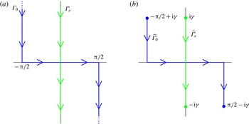
(a) The integration contours
 ${\it\Gamma}_{0}$
(blue solid) and
 ${\it\Gamma}_{\mathit{e}}$
(green dashed) in the complex
 ${\it\chi}$
-plane, which describe the domains of the amplitude functions
 $A_{m;q}^{\pm }({\it\chi})$
for travelling (
 $m=0$
) and evanescent (
 $m\geqslant 1$
) vertical modes respectively. The arrows indicate the directions of the contours. (b) The corresponding truncated contours
 $\widetilde{{\it\Gamma}}_{0}$
(blue solid) and
 $\widetilde{{\it\Gamma}}_{\mathit{e}}$
(green dashed) used in the numerical approximation discussed in § 3.2.

The integration contour
 ${\it\Gamma}_{m}$
differs for the travelling (
 $m=0$
) and evanescent (
 $m\geqslant 1$
) modes. For a travelling mode, it runs from
 $-{\rm\pi}/2+\text{i}\infty$
to
 ${\rm\pi}/2-\text{i}\infty$
through the origin and is parameterized by
 $$\begin{eqnarray}{\it\chi}({\it\varsigma})=\left\{\begin{array}{@{}cc@{}}-{\rm\pi}/2-\text{i}(1+{\it\varsigma}) & (-\infty \leqslant {\it\varsigma}\leqslant -1),\\ {\rm\pi}/2{\it\varsigma} & (-1\leqslant {\it\varsigma}\leqslant 1),\\ {\rm\pi}/2+\text{i}(1-{\it\varsigma}) & (1\leqslant {\it\varsigma}\leqslant \infty ).\end{array}\right.\end{eqnarray}$$
The contour
 ${\it\Gamma}_{0}$
is depicted in figure 2(a) as a blue solid line. The integration contours
 ${\it\Gamma}_{m}$
(
 $m\geqslant 1$
) for the evanescent vertical modes are all identically equal to
 ${\it\Gamma}_{\mathit{e}}$
, which spans the imaginary axis from
 $\text{i}\infty$
to
 $-\text{i}\infty$
, as shown in figure 2 (see the green dashed line in a). The integration contours
 ${\it\Gamma}_{0}$
and
 ${\it\Gamma}_{\mathit{e}}$
arise from decomposing a surface wave source into a superposition of plane waves continuously depending on the complex angular parameter
 ${\it\chi}$
, as will be shown in § 3.1.
The complex branches of
 ${\it\Gamma}_{0}$
correspond to wave components that decay exponentially in the
 $x$
-direction. The rate of decay increases as the imaginary components of
 ${\it\chi}$
get larger. In this regard, these components are similar to the evanescent modes.
We introduce an approximation for computational purposes, by truncating
 ${\it\Gamma}_{\mathit{e}}$
and the complex branches of
 ${\it\Gamma}_{0}$
to
 $\pm {\it\gamma}\text{i}$
and
 $\pm ({\rm\pi}/2-{\it\gamma}\text{i})$
respectively, where
 ${\it\gamma}\geqslant 0$
. The truncated contours are denoted by
 $\widetilde{{\it\Gamma}}_{0}$
and
 $\widetilde{{\it\Gamma}}_{\mathit{e}}$
and are shown in figure 2(b). It should be noted that the special case
 ${\it\gamma}=0$
represents a far-field approximation, for which all
 $x$
-decaying wave components are neglected in interactions between slabs. Its validity depends on the spacing between slabs and will be discussed further in § 4.
3.1. Reflection and transmission by a single slab
Montiel, Squire & Bennetts (Reference Montiel, Squire and Bennetts2015b
) derived a set of relationships (for the special case
 ${\it\gamma}=0$
) between the incident and scattered amplitude functions
 $A_{0;q}^{\pm }({\it\chi})$
on either side of a given slab
 $q$
as a result of reflection and transmission. Here, we extend these relationships to include evanescent vertical modes (i.e.
 $m\geqslant 1$
) and
 $x$
-decaying wave components (i.e.
 ${\it\gamma}>0$
).
We consider the scattering by slab
 $q$
due to the incident forcing from its left-hand side,
 ${\it\phi}_{q-1}^{(+)}$
, only. The response to incident forcing from its right-hand side,
 ${\it\phi}_{q}^{(-)}$
, follows similarly, and the total response to forcing from both sides is calculated via superposition.
The forcing field may be expressed in the local polar coordinates of floe
 $p$
analogously to (2.8a
). For each angular mode
 $n$
and vertical mode
 $m$
, the forcing amplitudes are then given by
 $$\begin{eqnarray}[\boldsymbol{f}_{n}^{(p)}]_{m}=\text{i}^{n}\int _{{\it\Gamma}_{m}}A_{m;q-1}^{+}({\it\chi})\text{e}^{-\text{i}n{\it\chi}}\text{e}^{\text{i}k_{m}((x_{p}-{\it\xi}_{q-1})\cos {\it\chi}+y_{p}\sin {\it\chi})}\,\text{d}{\it\chi}.\end{eqnarray}$$
The self-consistent method outlined in § 2.3 is used to solve the multiple scattering problem within the slab. It results in a system of equations analogous to (2.12) which yields the mapping
 $$\begin{eqnarray}\boldsymbol{b}^{[q]}=\unicode[STIX]{x1D63F}^{[q]}\boldsymbol{f}^{[q]},\end{eqnarray}$$
where
 $\boldsymbol{b}^{[q]}$
(
 $\boldsymbol{f}^{[q]}$
) is a vector of length
 $(M_{2}+1)(2N+1)N_{q}$
that contains all of the scattered (incident) wave amplitudes contained in
 $\boldsymbol{b}_{n}^{(p)}$
(
 $\boldsymbol{f}_{n}^{(p)}$
), for
 $-N\leqslant n\leqslant N$
and
 $1\leqslant p\leqslant N_{q}$
. The square matrix
 $\unicode[STIX]{x1D63F}^{[q]}$
has size
 $(M_{2}+1)(2N+1)N_{q}$
and is the DTM of slab
 $q$
.
We seek the reflected and transmitted amplitude functions in the form
 $$\begin{eqnarray}A_{m,q-1}^{-}({\it\chi})=\mathop{\sum }_{l=0}^{M_{2}}\int _{{\it\Gamma}_{l}}\mathscr{R}_{m,l;q}^{+}({\it\chi}\,:\,{\it\tau})A_{l;q-1}^{+}({\it\tau})\,\text{d}{\it\tau}\end{eqnarray}$$
and
 $$\begin{eqnarray}A_{m,q}^{+}({\it\chi})=\mathop{\sum }_{l=0}^{M_{2}}\int _{{\it\Gamma}_{l}}\mathscr{T}_{m,l;q}^{+}({\it\chi}\,:\,{\it\tau})A_{l;q-1}^{+}({\it\tau})\,\text{d}{\it\tau}\end{eqnarray}$$
respectively. The functions
 $\mathscr{R}_{m,l;q}^{+}({\it\chi}\,:\,{\it\tau})$
and
 $\mathscr{T}_{m,l;q}^{+}({\it\chi}\,:\,{\it\tau})$
are respectively reflection and transmission kernels for each pair of vertical modes
 $m$
and
 $l$
.
In order to evaluate the reflection and transmission kernels, we re-express the scattered wave field (2.8b ) due to each floe in the slab as a superposition of plane waves. This is achieved using the following plane wave representation of the outgoing cylindrical harmonics:
 $$\begin{eqnarray}\text{H}_{n}(k_{m}r)\text{e}^{\text{i}n{\it\theta}}=\left\{\begin{array}{@{}ll@{}}\displaystyle \frac{(-\text{i})^{n}}{{\rm\pi}}\int _{{\it\Gamma}_{m}}\text{e}^{\text{i}n{\it\chi}}\text{e}^{\text{i}k_{m}(x\cos {\it\chi}+y\sin {\it\chi})}\,\text{d}{\it\chi} & (x\geqslant 0),\\ \displaystyle \frac{\text{i}^{n}}{{\rm\pi}}\int _{{\it\Gamma}_{m}}\text{e}^{-\text{i}n{\it\chi}}\text{e}^{\text{i}k_{m}(-x\cos {\it\chi}+y\sin {\it\chi})}\,\text{d}{\it\chi} & (x\leqslant 0),\end{array}\right.\end{eqnarray}$$
where
 $(x,y)=(r\cos {\it\theta},r\sin {\it\theta})$
. This identity is derived from Sommerfeld’s integral representation of the Hankel function (Sommerfeld Reference Sommerfeld1949) for
 $m=0$
, while an integral representation of the modified Bessel functions of the second kind
 $\text{K}_{n}$
has been used for
 $m\geqslant 1$
(see Linton & Evans Reference Linton and Evans1992, equation (2.12)). To the best of the authors’ knowledge, the two cases have not been unified in this manner before. By substituting (3.7) into (2.8b
) for all floes and modes simultaneously, and using (3.5) and (3.4) in turn, we obtain the following semianalytical expressions for the reflection and transmission kernels after algebraic manipulations:
 $$\begin{eqnarray}\mathscr{R}_{m,l;q}^{+}({\it\chi}\,:\,{\it\tau})=(\boldsymbol{v}_{m;q}^{\mathit{S}-}({\it\chi}))^{\mathit{tr}}\unicode[STIX]{x1D64B}\unicode[STIX]{x1D63F}^{[q]}\unicode[STIX]{x1D64B}^{-1}\boldsymbol{v}_{l;q}^{\mathit{In}+}({\it\tau})\end{eqnarray}$$
and
 $$\begin{eqnarray}\mathscr{T}_{m,l;q}^{+}({\it\chi}\,:\,{\it\tau})=(\boldsymbol{v}_{m;q}^{\mathit{S}+}({\it\chi}))^{\mathit{tr}}\unicode[STIX]{x1D64B}\unicode[STIX]{x1D63F}^{[q]}\unicode[STIX]{x1D64B}^{-1}\boldsymbol{v}_{l;q}^{\mathit{In}+}({\it\tau})+\text{e}^{\text{i}k_{m}L_{q}\cos {\it\chi}}{\it\delta}({\it\chi}-{\it\tau}),\end{eqnarray}$$
where a superscript
 $tr$
indicates transpose and
 ${\it\delta}(\cdot )$
denotes the Dirac delta.
In these expressions we have defined the vector
 $\boldsymbol{v}_{l;q-1}^{\mathit{In}+}({\it\tau})$
of length
 $N_{q}(2N+1)$
 $(M_{2}+1)$
, which provides a change from Cartesian to polar coordinates of the forcing field in the local system of each floe in the slab. Its entries are
 $$\begin{eqnarray}[\boldsymbol{v}_{m;q}^{\mathit{In}+}({\it\tau})]_{\mathit{ind}(l,p,n)}=\text{i}^{n}\text{e}^{-\text{i}n{\it\tau}}\text{e}^{\text{i}k_{l}((x_{p}-{\it\xi}_{q-1})\cos {\it\tau}+y_{p}\sin {\it\tau})}{\it\delta}_{m\,l},\end{eqnarray}$$
where
 $\mathit{ind}(l,p,n)=lN_{q}(2N+1)+(p-1)(2N+1)+N+n+1$
defines the modal hierarchy (vertical mode, floe number, angular mode) in ordering entries, and
 ${\it\delta}_{m\,l}$
is the Kronecker delta. In contrast, the vectors
 $\boldsymbol{v}_{m;q-1}^{\mathit{S}-}({\it\chi})$
and
 $\boldsymbol{v}_{m;q}^{\mathit{S}+}({\it\chi})$
provide a change from polar to Cartesian coordinates of the scattered field due to each floe, travelling in the leftward and rightward direction respectively. Their entries are
 $$\begin{eqnarray}[\boldsymbol{v}_{m;q}^{\mathit{S}-}({\it\chi})]_{\mathit{ind}(l,p,n)}=\frac{\text{i}^{n}}{{\rm\pi}}\text{e}^{-\text{i}n{\it\chi}}\text{e}^{\text{i}k_{l}((x_{p}-{\it\xi}_{q-1})\cos {\it\chi}-y_{p}\sin {\it\chi})}{\it\delta}_{m\,l}\end{eqnarray}$$
and
 $$\begin{eqnarray}[\boldsymbol{v}_{m;q}^{\mathit{S}+}({\it\chi})]_{\mathit{ind}(l,p,n)}=\frac{(-\text{i})^{n}}{{\rm\pi}}\text{e}^{\text{i}n{\it\chi}}\text{e}^{-\text{i}k_{l}((x_{p}-{\it\xi}_{q})\cos {\it\chi}+y_{p}\sin {\it\chi})}{\it\delta}_{m\,l}.\end{eqnarray}$$
The matrix
 $\unicode[STIX]{x1D64B}$
is a permutation matrix of size
 $N_{q}(2N+1)(M_{2}+1)$
used to change the modal hierarchy from that used in the slab DTM
 $\unicode[STIX]{x1D63F}^{[q]}$
(i.e. floe number, angular mode, vertical mode) to that used in (3.9). It should also be noted that the second term in (3.8b
) represents the contribution from the forcing field to the transmitted field.
3.2. Multiple slabs
At the boundary
 $x={\it\xi}_{q}$
, the left- and right-travelling amplitude functions take the form
 $$\begin{eqnarray}A_{m,q}^{-}({\it\chi})=\mathop{\sum }_{l=0}^{M_{2}}\int _{{\it\Gamma}_{l}}(\mathscr{R}_{m,l;q+1}^{+}({\it\chi}\,:\,{\it\tau})A_{l;q}^{+}({\it\tau})+\mathscr{T}_{m,l;q+1}^{-}({\it\chi}\,:\,{\it\tau})A_{l;q+1}^{-}({\it\tau}))\,\text{d}{\it\tau}\end{eqnarray}$$
and
 $$\begin{eqnarray}A_{m,q}^{+}({\it\chi})=\mathop{\sum }_{l=0}^{M_{2}}\int _{{\it\Gamma}_{l}}(\mathscr{T}_{m,l;q}^{+}({\it\chi}\,:\,{\it\tau})A_{l;q-1}^{+}({\it\tau})+\mathscr{R}_{m,l;q}^{-}({\it\chi}\,:\,{\it\tau})A_{l;q}^{-}({\it\tau}))\,\text{d}{\it\tau},\end{eqnarray}$$
where the kernel functions
 $\mathscr{R}_{m,l;q}^{\pm }$
and
 $\mathscr{T}_{m,l;q}^{\pm }$
are found using the method described in § 3.1. Given that the forcing is provided by (2.4) only, we have
 $A_{0;0}^{+}({\it\chi})=A^{\mathit{In}}({\it\chi})$
,
 $A_{0;m}^{+}({\it\chi})=0$
for
 $1\leqslant m\leqslant M_{2}$
and
 $A_{S;m}^{-}({\it\chi})=0$
for
 $0\leqslant m\leqslant M_{2}$
.
A numerical scheme is implemented by discretizing the amplitude and kernel functions using a uniform sampling of the angular parameters
 ${\it\chi}$
and
 ${\it\tau}$
. Amplitudes and kernels associated with a travelling vertical mode (
 $m=0$
) are defined on the truncated contour
 $\widetilde{{\it\Gamma}}_{0}$
introduced at the beginning of § 3 (see figure 2
b). Contour
 $\widetilde{{\it\Gamma}}_{0}$
is then discretized by selecting
 $2N_{\mathit{tr}}+1$
samples
 ${\it\chi}_{i}$
,
 $-N_{\mathit{tr}}\leqslant i\leqslant N_{\mathit{tr}}$
. Different resolutions are taken for the subinterval
 $[-{\rm\pi}/2,{\rm\pi}/2]$
of
 $\widetilde{{\it\Gamma}}_{0}$
and its complex branches. Typically, the resolution chosen for the complex branches is five times as coarse as that of
 $[-{\rm\pi}/2,{\rm\pi}/2]$
. Likewise, contour
 $\widetilde{{\it\Gamma}}_{\mathit{e}}$
is discretized using
 $2N_{\mathit{ev}}+1$
samples.
Combining all the vertical modes, we can define vector versions of the amplitude functions
 $\boldsymbol{A}_{q}^{\pm }$
containing the value of the corresponding continuous functions
 $A_{m,q}^{\pm }({\it\chi}_{i})$
at all angular samples
 ${\it\chi}_{i}$
. Likewise, we obtain matrix versions of the kernel functions after discretization. At this point, a numerical quadrature must be chosen to approximate the integrals involved in (3.10). Although high-order schemes, e.g. Simpson’s rule or Gaussian quadrature, are very accurate for relatively smooth functions, we expect our spectra to be noisy for large random arrays of floes (confirmed by numerical experiments), in which case lower-order quadratures provide more accurate and more efficient estimates. We found that a composite trapezoidal rule gave the best results in terms of convergence. The weighting factors of the trapezoidal rule can be assembled in a diagonal matrix of size
 $N_{\mathit{ang}}=2N_{\mathit{tr}}+1+M_{2}(2N_{\mathit{ev}}+1)$
, which multiplies the matrix versions of the kernel functions to give the reflection and transmission matrices
 $\unicode[STIX]{x1D64D}_{q}^{\pm }$
and
 $\unicode[STIX]{x1D64F}_{q}^{\pm }$
. Consequently, (3.10) is written in the discretized form
 $$\begin{eqnarray}\boldsymbol{A}_{q}^{-}=\unicode[STIX]{x1D64D}_{q+1}^{+}\boldsymbol{A}_{q}^{+}+\unicode[STIX]{x1D64F}_{q+1}^{-}\boldsymbol{A}_{q+1}^{-}\quad \text{and}\quad \boldsymbol{A}_{q}^{+}=\unicode[STIX]{x1D64F}_{q}^{+}\boldsymbol{A}_{q-1}^{+}+\unicode[STIX]{x1D64D}_{q}^{-}\boldsymbol{A}_{q}^{-}.\end{eqnarray}$$
The solution to the slab interaction problem is obtained using an efficient iterative technique, which is an extension to the one described by Montiel et al. (Reference Montiel, Squire and Bennetts2015a
) for travelling modes only. Following this approach, at each slab boundary
 $x={\it\xi}_{q}$
, the unknown amplitude vectors are given by
 $$\begin{eqnarray}\boldsymbol{A}_{q}^{+}=\left(\unicode[STIX]{x1D644}-\unicode[STIX]{x1D64D}_{1,q}^{-}\unicode[STIX]{x1D64D}_{q+1,M}^{+}\right)^{-1}\unicode[STIX]{x1D64F}_{1,q}^{+}\boldsymbol{A}_{0}^{+}\end{eqnarray}$$
and
 $$\begin{eqnarray}\boldsymbol{A}_{q}^{-}=\left(\unicode[STIX]{x1D644}-\unicode[STIX]{x1D64D}_{q+1,M}^{+}\unicode[STIX]{x1D64D}_{1,q}^{-}\right)^{-1}\unicode[STIX]{x1D64D}_{q+1,M}^{+}\unicode[STIX]{x1D64F}_{1,q}^{+}\boldsymbol{A}_{0}^{+},\end{eqnarray}$$
where
 $\unicode[STIX]{x1D644}$
denotes the identity matrix of order
 $N_{\mathit{ang}}$
, and
 $\unicode[STIX]{x1D64D}_{p,q}^{\pm }$
and
 $\unicode[STIX]{x1D64F}_{p,q}^{\pm }$
are the reflection and transmission matrices respectively for the stack of slabs
 $p$
to
 $q$
. These reflection and transmission matrices are computed iteratively, starting from slab 1 alone, which initializes the procedure, to the stack of slabs 1 to
 $S$
, adding one slab to the stack at each iteration.
We establish a convergence criterion for the numerical integration scheme considered here, based on the energy conservation relation
 $$\begin{eqnarray}\int _{-{\rm\pi}/2}^{{\rm\pi}/2}|A^{\mathit{R}}({\it\chi})|^{2}\,\text{d}{\it\chi}+\int _{-{\rm\pi}/2}^{{\rm\pi}/2}|A^{\mathit{T}}({\it\chi})|^{2}\,\text{d}{\it\chi}=\int _{-{\rm\pi}/2}^{{\rm\pi}/2}|A^{\mathit{In}}({\it\chi})|^{2}\,\text{d}{\it\chi}\end{eqnarray}$$
being satisfied within a tolerance of
 $10^{-4}$
, where the reflected and transmitted amplitude functions are given by
 $A^{\mathit{R}}({\it\chi})=A_{0;0}^{-}({\it\chi})$
and
 $A^{\mathit{T}}({\it\chi})=A_{0;S}^{+}({\it\chi})$
respectively for
 $-{\rm\pi}/2\leqslant {\it\chi}\leqslant {\rm\pi}/2$
. It should be noted that we have restricted the integration domain to include travelling wave components only, as they are the only ones to affect the energy balance of the system. We refer to the restriction of the amplitude functions
 $A_{0;q}^{\pm }({\it\chi})$
,
 $q=0,\ldots ,S$
, to
 $-{\rm\pi}/2\leqslant {\it\chi}\leqslant {\rm\pi}/2$
as directional spectra. In particular,
 $A^{\mathit{R}}({\it\chi})$
and
 $A^{\mathit{T}}({\it\chi})$
are the reflected and transmitted directional spectra respectively.
We further note that although the energy conservation relation (3.13) is necessary for convergence of our numerical method, it is not sufficient to obtain convergence to the desired solution. In particular, we can always obtain energy conservation for sufficiently high
 $N_{\mathit{ang}}$
, regardless of the value taken for the truncation parameter
 ${\it\gamma}$
and the resolution of the complex branches in our numerical approximation of the integration contours
 $\widetilde{{\it\Gamma}}_{\mathit{e}}$
and
 $\widetilde{{\it\Gamma}}_{0}$
. Convergence of the solution within the desired tolerance is obtained for a sufficiently large
 ${\it\gamma}$
, as will be shown in § 4.
4. Far-field approximations
The far-field approximations neglect evanescent/decaying wave components in wave interactions between floes. The first far-field approximation (FFA1) we consider consists of neglecting the vertical evanescent modes (i.e. setting
 $M_{2}=0$
) to calculate wave interactions between floes in the slabs. To the best of the authors’ knowledge, the convergence properties of the self-consistent approach for wave interactions between floes with respect to the number of vertical modes used have not been investigated previously. In comparison, the convergence properties of the EMM for a single floe with respect to the vertical modes are well understood (see, e.g., Montiel Reference Montiel2012).
Consider a large array of 20 slabs, each containing 51 identical floes with radius
 $a=150~\text{m}$
and thickness
 $D=1.5~\text{m}$
. The relatively large floes in this array test the convergence properties of the method to a greater extent than the range of floe radii in the natural FSDs used in the simulations presented in § 6. The floes are assumed to be equally spaced and aligned in both the
 $x$
- and
 $y$
-directions, forming a regular square grating symmetric about the
 $x$
-axis. We define the non-dimensional spacing of the grating as the ratio of the centre-to-centre distance between two adjacent floes and the floe diameter. It is denoted by
 ${\it\sigma}$
and equals
 $L/2a\geqslant 1$
, where
 $L=L_{1}=\cdots =L_{q}$
is the width of the slabs. We prescribe the incident directional spectrum
 $A^{\mathit{In}}({\it\tau})=\cos {\it\tau}$
, the wave period
 $T=2{\rm\pi}/{\it\omega}$
and set the fluid depth to
 $h=200~\text{m}$
. We define the reflection coefficient of the array to be
 $$\begin{eqnarray}R=\sqrt{\left(\int _{-{\rm\pi}/2}^{{\rm\pi}/2}|A^{\mathit{R }}({\it\chi})|^{2}\,\text{d}{\it\chi}\right)\bigg/\left(\int _{-{\rm\pi}/2}^{{\rm\pi}/2}|A^{\mathit{In }}({\it\chi})|^{2}\,\text{d}{\it\chi}\right)}.\end{eqnarray}$$
It is used to analyse the convergence with respect to the vertical modes.
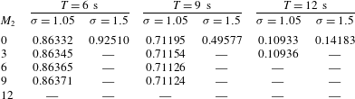
Table 1 shows values (to five significant digits) of the reflection coefficient for the three wave periods
 $T=6,9$
and
 $12~\text{s}$
, and two spacings
 ${\it\sigma}=1.05$
(dense array) and
 $1.5$
(loose array). It indicates that floe spacing is the dominant influence on the rate of convergence with respect to the number of vertical modes used. For the loose array (large spacing), all evanescent waves decay rapidly and do not interact with adjacent floes for all wave periods considered, as the reflection coefficient is accurate to five digits with the FFA1 (
 $M_{2}=0$
). For the dense array,
 $M_{2}=9$
evanescent modes are required to reach five-digit accuracy for the two shorter wave periods,
 $T=6$
and 9 s, while only
 $M_{2}=3$
evanescent modes are needed for longer waves (
 $T=12~\text{s}$
). Shorter waves are expected to experience more scattering and therefore to generate more intense evanescent modes than longer waves, which is consistent with our observations. It should also be noted that the FFA1 provides three-digit accuracy for all wave periods in the dense array case, which is the level of accuracy sought as part of this investigation. It is thus reasonable to consider the FFA1 valid for at least
 $T\geqslant 6~\text{s}$
for the array considered here or
 $ka\leqslant 16$
more generally. Consequently, the FFA1 will be invoked for the remainder of this paper.
Convergence of the reflection coefficient with respect to the number of vertical modes
 $M_{2}$
for three wave periods (
 $T=6,\,9$
and
 $12~\text{s}$
) and two grating spacings (
 ${\it\sigma}=1.05$
and
 $1.5$
). A long dash signifies a value identical to the one directly above.

In § 3 the integral expressions for the wave fields at the slab boundaries were approximated by discretizing the parameterized contours
 ${\it\Gamma}_{0}$
and
 ${\it\Gamma}_{\mathit{e}}$
. Specifically, the complex branches were truncated to
 $\pm ({\rm\pi}/2-{\it\gamma}\text{i})$
for
 ${\it\Gamma}_{0}$
and
 $\pm {\it\gamma}\text{i}$
for
 ${\it\Gamma}_{\mathit{e}}$
. The value taken for the truncation parameter
 ${\it\gamma}$
determines the proportion of
 $x$
-decaying wave components taken into account for a slab. These decaying waves do not affect the far-field solution (
 $|x|\rightarrow \infty$
) of the single-slab problem. Therefore, a second far-field approximation (FFA2) is proposed, in which the
 $x$
-decaying wave components are neglected in the interactions between slabs, i.e. we set
 ${\it\gamma}=0$
. We investigate the validity of FFA2 below which, to the best of the authors’ knowledge, has not been been conducted before.
We consider the same 20-slab arrays as in the previous analysis. The problem is solved for increasing values of
 ${\it\gamma}$
with
 $0\leqslant {\it\gamma}\leqslant 2.5$
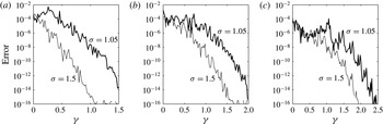
. The accuracy of the solution is estimated by the absolute error between successively calculated values of the reflection coefficients. These are plotted in figure 3 for wave periods
 $T=6$
,
 $9$
and
 $12~\text{s}$
, and grating spacings
 ${\it\sigma}=1.05$
and
 $1.5$
. Although the error curves are all noisy, we detect clear convergence trends. Error estimates all reach machine precision within the interval
 $0\leqslant {\it\gamma}\leqslant 2.5$
, but the convergence rate depends strongly on both wave period and spacing. In particular, faster convergence is observed at shorter wave periods for a given spacing, while the denser array tends to slow the convergence for each period. In all cases considered here, a
 $10^{-5}$
error (four-digit accuracy) is reached with
 ${\it\gamma}\approx 1.2$
. Therefore, we will use this value for the remainder of our investigation, i.e. we do not employ FFA2.
Estimated error on values of the reflection coefficient against the truncation parameter
 ${\it\gamma}$
. The convergence analysis is conducted for (a)
 $T=6~\text{s}$
, (b) 9 s and (c)
 $12~\text{s}$
, and two grating spacings.

5. Simulations and randomness
5.1. Random sea states
We model the forcing wave field as a random directional sea state, in which wave components travelling at different angles do not interfere coherently, i.e. their phases are uncorrelated. Numerical tests (not shown here) indicate that the reflection properties of an array of floes depend strongly on the directional coherence of the forcing field. Specifically, the reflection coefficient (and therefore the attenuation rate of wave energy) computed for a coherent forcing field is typically higher than that obtained for an incoherent field with the same prescribed incident spectrum. In addition to incoherence, we require the simulated directional sea state to be ergodic in the sense that the wave statistics over the spatial domain are uniform and can be deduced from its properties at a single point in the domain. This property is needed to reduce the variability of the response of the system to a random forcing, as will be discussed below.
A number of methods exist to simulate ergodic directional sea states deterministically (see, e.g., Jefferys Reference Jefferys1987; Miles & Funke Reference Miles and Funke1989). Most methods are based on multiple frequency wave spectra, for which a realization of the random sea state is generated by a double sum over the directional and frequency range of plane waves with random characteristics. As we assume a monochromatic wave forcing, the double sum is replaced by a single sum over
 $N_{\mathit{tr}}$
directions, giving a free-surface displacement
 $$\begin{eqnarray}{\it\eta}^{\mathit{In}}(x,y,t)=\mathop{\sum }_{i=1}^{N_{\mathit{tr}}}a_{i}\cos (k_{0}(x\cos {\it\tau}_{i}+y\sin {\it\tau}_{i})-{\it\omega}t+{\it\varepsilon}_{i}).\end{eqnarray}$$
For each wave component travelling at angle
 ${\it\tau}_{i}$
with respect to the
 $x$
-axis, the amplitude
 $a_{i}$
is defined deterministically from an energy spreading function
 $D({\it\tau})$
, and the phase
 ${\it\varepsilon}_{i}$
is a random parameter with uniform distribution between
 $0$
and
 $2{\rm\pi}$
. For the remainder of the investigation we prescribe a standard cosine-squared energy spreading function, i.e.
 $$\begin{eqnarray}D({\it\tau})=\frac{2}{{\rm\pi}}\cos ^{2}({\it\tau})\quad (-{\rm\pi}/2\leqslant {\it\tau}\leqslant {\rm\pi}/2),\end{eqnarray}$$
where the constant factor is chosen so that the total energy of the wave field is
 $$\begin{eqnarray}\int _{-{\rm\pi}/2}^{{\rm\pi}/2}D({\it\tau})\,\text{d}{\it\tau}=1.\end{eqnarray}$$
The energy spreading function (5.2) and the amplitudes of (5.1) are related by
 $a_{i}=\sqrt{2D({\it\tau}_{i}){\rm\Delta}{\it\tau}}$
for
 $1\leqslant i\leqslant N_{\mathit{tr}}$
in (5.1), with
 ${\rm\Delta}{\it\tau}={\rm\pi}/(N_{\mathit{tr}}-1)$
and
 ${\it\tau}_{i}=(i-1){\rm\Delta}{\it\tau}-{\rm\pi}/2$
.
Although directional incoherence is directly satisfied in (5.1) through the random parameter
 ${\it\varepsilon}_{i}$
, following Jefferys (Reference Jefferys1987) we show in appendix A that this equation does not simulate an ergodic field, i.e. much spatial variability exists in the mean energy of a generated sea state (
 ${\approx}100\,\%$
relative standard error). A simple remedy is to perform averaging over an ensemble of random realizations of the wave field. The method converges slowly, however, and approximately 10 000 realizations of the sea state are necessary to approximate ergodicity with 1 % relative standard error on the incident field mean energy.
We compute the corresponding reflected energy,
 $R^{2}$
, for the 20-slab grating considered in § 4, with spacing constant
 ${\it\sigma}=1.5$
. The forcing is defined by the random sea state (5.1) with period
 $T=9~\text{s}$
and an energy spreading function given by (5.2). Using an ensemble of 1000 realizations of the random forcing field, we calculated the relative standard error on a single estimate of the reflected energy to be approximately
 $7\,\%$
. Averaging over many realizations of the random wave forcing, the relative error of the average estimate then drops as the inverse square root of the number of realizations, so it is approximately
 $1\,\%$
for 50 realizations. This contrasts with the 10 000 simulations required to estimate the incident field mean energy with the same tolerance. Similar results were obtained for other wave periods. This analysis suggests that the scattering properties of large arrays have a low sensitivity to random variations in the phase of the wave forcing. For a regular array of ice floes, a relatively small number of random realizations of the sea state then suffices to obtain accurate estimates of the scattering properties of large arrays.
5.2. Simulation of a natural FSD
We model the MIZ as a randomly selected array of floes with different sizes, such that the diameters obey a power-law distribution, which is a standard empirical model of the FSD (see, e.g., Rothrock & Thorndike Reference Rothrock and Thorndike1984; Toyota et al. Reference Toyota, Takatsuji and Nakayama2006, Reference Toyota, Haas and Tamura2011). This is a unique feature of our three-dimensional attenuation model. Further, it allows us to simulate an MIZ with a high concentration, which would otherwise not be possible with a single floe size, e.g. the mean floe size.
We use an approach similar to that of Kohout & Bertino (Reference Dumont, Kohout and Bertino2011) and Williams et al. (Reference Williams, Bennetts, Squire, Dumont and Bertino2013a
) to parameterize the FSD, in which a bounded power-law distribution is used. We define the probability density function
 $(a/a_{\mathit{min}})^{-{\it\kappa}}$
for
 $a_{\mathit{min}}\leqslant a\leqslant a_{\mathit{max}}$
, where
 ${\it\kappa}$
is a constant parameter. Therefore, the probability that a floe has a radius
 $a<\mathfrak{a}$
is then given by
 $$\begin{eqnarray}\mathbb{P}(a<\mathfrak{a})=\frac{\mathfrak{a}^{1-{\it\kappa}}-a_{\mathit{min}}^{1-{\it\kappa}}}{a_{\mathit{max}}^{1-{\it\kappa}}-a_{\mathit{min}}^{1-{\it\kappa}}}.\end{eqnarray}$$
The distribution is then discretized so that a small finite number,
 $N_{b}$
say, of unique floe sizes is considered.
An algorithm to generate a distribution of ice floes in a slab using the bounded power-law FSD described here is described in appendix B. As the MIZ generated in our model is obtained by stacking together a large number of slabs, the same FSD is satisfied for the whole MIZ. The parameters of the algorithm are the dimensions of the ice-covered region in the slab, i.e. the width
 $L_{x}$
and breadth
 $L_{y}$
, the number of bins
 $N_{\mathit{b}}$
, the ice concentration
 $c$
, the minimum and maximum floe radii
 $a_{\mathit{min}}$
and
 $a_{\mathit{max}}$
, and the exponent in the power-law distribution
 ${\it\kappa}$
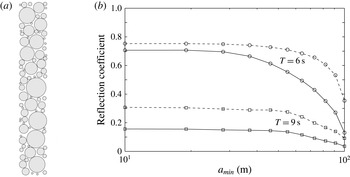
. An example of a random array generated using this algorithm is shown in figure 4(a) for parameter values
 $L_{x}=220~\text{m}$
,
 $L_{y}=8L_{x}$
,
 $N_{b}=11$
,
 $c=0.7$
,
 $a_{\mathit{min}}=10~\text{m}$
,
 $a_{\mathit{max}}=100~\text{m}$
and
 ${\it\kappa}=1.84$
. The last three parameters are the same as those used by Williams et al. (Reference Williams, Bennetts, Squire, Dumont and Bertino2013a
). This range of floe sizes is comparable to the floe sizes typically observed in real MIZs (see, e.g. Toyota et al.
Reference Toyota, Takatsuji and Nakayama2006).
To generate a highly concentrated MIZ, our algorithm populates each slab with a large number of small floes. The effect of these small floes on wave interactions is likely to be negligible, however, while it increases the computational cost of the self-consistent method used to calculate the multiple scattering within each slab. Accordingly, we devise below a numerical test to determine the minimum floe size
 $a_{\mathit{min}}$
contributing to scattering by a large array.
Consider a randomly selected array in a single slab parameterized as before, but with larger breadth
 $L_{y}=51L_{x}$
. The array generated contains 488 floes. We compute ensemble averages of the reflection coefficient
 $R$
due to random realizations of the incident sea state with an energy spreading function given by (5.2). The calculations are repeated after removing all of the floes with the smallest floe size successively until
 $a_{\mathit{min}}=a_{\mathit{max}}$
, in which case the concentration is approximately
 $5\,\%$
.
(a) Example of array generated using the random array generator described in appendix B. (b) Ensemble averages of reflection coefficients plotted against the minimum floe radius of the power-law FSD used to generate random realizations of the arrays. Results are given for single- and 10-slab arrays (solid and dashed lines respectively) and wave periods
 $T=6$
and 9 s (circle and square markers respectively). The wave forcing is a random sea state with normalized cosine square energy spreading.

Figure 4 shows ensemble averages of the reflection coefficient against the minimum floe radius
 $a_{\mathit{min}}$
, for wave periods
 $T=6$
and 9 s (solid lines with circle and square markers respectively). Each data point is calculated as the average of 100 simulations, each of which is characterized by a random realization of the array and the incident sea state. For small
 $a_{\mathit{min}}$
, the reflection coefficient remains roughly constant for both wave periods considered, suggesting that very small floes do not influence the scattering properties of the slab. A change of regime occurs for
 $a_{\mathit{min}}\approx 28~\text{m}$
at
 $T=6~\text{s}$
and
 $a_{\mathit{min}}\approx 55~\text{m}$
at
 $T=9~\text{s}$
, beyond which the reflection coefficient decreases as
 $a_{\mathit{min}}$
increases, so that the smallest floes start to contribute to scattering by the slab. These values of
 $a_{\mathit{min}}$
are used to define the critical minimum floe size
 $D_{\mathit{crit}}=2a_{\mathit{min}}$
, corresponding to the change of regime described above.
Our estimates of the critical minimum floe size,
 $D_{\mathit{crit}}\approx 56$
and
 $110~\text{m}$
, are similar to the corresponding open water wavelengths,
 ${\it\lambda}_{0}=2{\rm\pi}/k_{0}\approx 56$
and
 $126~\text{m}$
, for
 $T=6$
s and 9 s respectively. This suggests that scattering by floes smaller than the forcing wavelength is negligible and that these floes need not be included in the FSD.
We repeat the analysis for arrays composed of 10 slabs. To reduce the computing time, we solve the single-slab problem for 50 random realizations of the array and then perform random permutations of the pool of single-slab arrays to generate random 10-slab arrays (the validity of this approach will be discussed in § 5.3). Ensemble averages of the reflection coefficient for varying
 $a_{\mathit{min}}$
are plotted in figure 4 for
 $T=6$
and 9 s (dashed lines with circle and square markers respectively). We observe a two-regime dependence on
 $a_{\mathit{min}}$
, similar to the single-slab array, with
 $D_{\mathit{crit}}$
taking the same value for both wave periods, noting that the transition between the regimes is much smoother for
 $T=6~\text{s}$
. We deduce that the critical minimum floe size does not depend on the size of the array but seems to be an intrinsic property of the FSD, varying with wave period and possibly ice thickness (not studied here).
5.3. Averaging
The multiple-slab interaction technique described in § 3.2 performs efficiently as the computational cost depends linearly on the number of slabs. Computing the reflection and transmission matrices of each slab is more time-consuming, however, as a 2D multiple scattering problem, which is
 $O(N_{q}^{3})$
expensive, needs to be solved for each slab
 $q$
containing
 $N_{q}$
floes. To reduce the number of single-slab solutions to compute, we calculate the reflection and transmission matrices of a fixed number
 $S_{u}$
of unique slabs and store them, requiring
 $O(S_{u}N_{\mathit{ang}}^{2})$
memory space. Each realization of a multiple-slab array is then generated from random permutations (allowing repetitions) of the
 $S_{u}$
unique slabs. Bennetts (Reference Bennetts2011) used this method in a related acoustic problem, where each slab was composed of an infinite regular array of scatterers with different in-row spacings, and found that
 $S_{u}=50$
was sufficient to take ensemble averages of wave transmission by 100-slab arrays. In our case, the slabs contain only a finite number of scatterers, and the scatterers are of different sizes and not positioned in a regular manner. Therefore, it is unclear whether a value of
 $S_{u}$
similar to that of Bennetts (Reference Bennetts2011) will be appropriate.
We devised a numerical test to determine a suitable value of
 $S_{u}$
. Consider a 100-slab array with slab dimensions
 $L_{x}=220~\text{m}$
and
 $L_{y}=51L_{x}$
, and an FSD in each slab parameterized as in § 5.2. We compute the reflection coefficient of the array for different values
 $S_{u}$
at wave periods
 $T=6$
and 9 s with
 $a_{\mathit{min}}=37$
and
 $55~\text{m}$
respectively (using our findings from § 5.2). For each value of
 $S_{u}$
considered, a single sample of
 $S_{u}$
unique slabs is generated to perform random permutations, and independent samples are used for different values of
 $S_{u}$
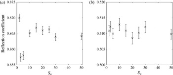
. Each computed value of the reflection coefficient is the mean of an ensemble of 50 realizations of the array, where each realization is obtained by randomly permuting unique slabs from the same sample of slabs generated. The results of these computations are shown in figure 5, where error bars indicate the standard error of the mean.
Ensemble average of the reflection coefficient by a 100-slab array computed for different values of
 $S_{u}$
. The array in each unique slab is generated using the FSD described in § 5.2 with dimensions
 $L_{x}=220~\text{m}$
and
 $L_{y}=51L_{x}$
. Results are shown for (a)
 $T=6~\text{s}$
and (b)
 $T=9~\text{s}$
. Averages are computed from 50 random realizations of the array and wave forcing (with a cosine square spread).

We observe a remarkable consistency in the computed values of the reflection coefficient, with two significant digit accuracy being obtained even for a small number of unique slabs, i.e.
 $S_{u}=10$
and
 $2$
for
 $T=6$
s and 9 s respectively. Specifically, the standard error of the mean values of
 $R$
for
 $S_{u}\geqslant 10$
and
 $2$
(for
 $T=6$
s and 9 s respectively) is
 ${<}0.1\,\%$
. It should be noted that each point is computed using an independent set of unique slabs, so that points obtained with different values of
 $S_{u}$
are uncorrelated. This suggests that a small value of
 $S_{u}$
is sufficient to simulate scattering by large random arrays of floes. In particular, the heterogeneity introduced in each unique slab (random floe packing) translates to larger scales when the slabs are stacked together. We fix
 $S_{u}=10$
for the remainder of the investigation, so that the memory space required to store the reflection and transmission matrices is
 $O(N_{\mathit{ang}}^{2})$
.
We also find that the procedure is very accurate, as each estimate of the reflection coefficient (i.e. for a single random realization of the array and wave forcing) has a relative standard error of the mean of approximately 2.5 and 1 % for
 $T=6$
s and 9 s respectively. Therefore, after averaging over 50 random realizations, the error drops to approximately 0.35 % and 0.15 % (respectively). We account for some variability in the values of
 $R$
for
 $S_{u}\geqslant 10$
by reducing the ensemble size used to average. Specifically, we use an ensemble of 10 random realizations, which gives a relative standard error below
 $1\,\%$
for both wave periods.
6. Attenuation and directional spreading
We describe wave energy attenuation and directional spreading through the MIZ by considering the evolution of the forward propagating directional wave field. Backward propagating wave components are not analysed here because their dependence on the finite extent of the simulated MIZ distorts the rate of energy decay – the larger the array the more backscattered wave energy exists across the array, until full reflection,
 $R=1$
, is achieved. However, these backward travelling components affect the attenuation and directional spreading of the forward propagating components. In particular, the limited extent of the MIZ in the
 $x$
-direction minimizes backward components near the end of the array, which in turn accelerates the attenuation rate of forward wave energy (discussed subsequently).
At each slab boundary
 $x={\it\xi}_{q}$
,
 $q=0,\ldots ,S$
, the wave energy of the forward propagating components is defined by
 $$\begin{eqnarray}E^{+}(x_{q})=\int _{-{\rm\pi}/2}^{{\rm\pi}/2}S_{q}^{+}({\it\chi})\,\text{d}{\it\chi},\quad \text{where }S_{q}^{+}({\it\chi})=|A_{0,q}^{+}({\it\chi})|^{2}\end{eqnarray}$$
is a directional energy density function. It should be noted that
 $S_{q}^{+}({\it\chi})$
characterizes the directional energy density of the forward propagating components on the line
 $x={\it\xi}_{q}$
, as opposed to at the point
 $(x,y)=({\it\xi}_{q},0)$
.
The method to extract wave energy attenuation and directional spreading is demonstrated on a case study parameterized to represent a realistic MIZ, as described in § 5.2. Consider an array of ice floes composed of
 $S=220$
slabs formed by random permutations of
 $S_{u}=10$
unique slabs. Each unique slab is parameterized with
 $L_{x}=220~\text{m}$
,
 $L_{y}=220\times L_{x}$
,
 $c=0.7$
,
 $N_{b}=19$
,
 $D=1.5~\text{m}$
(for all floes),
 $a_{\mathit{min}}=10~\text{m}$
,
 $a_{\mathit{max}}=100~\text{m}$
and
 ${\it\kappa}=1.84$
, so that the extent of the simulated MIZ is approximately
 $50~\text{km}\times 50~\text{km}$
. For all wave periods, we then remove from the array the floes with a radius smaller than
 $35~\text{m}$
, which have negligible effects on the evolution of wave properties. The forcing is given by a normalized cosine-squared directional sea state, as described in § 5.1. We consider the range of wave periods
 $T=6$
–15 s.
We implement an averaging procedure over 10 random realizations of the array and wave forcing. For each realization: (i) we generate independent random copies of the array and the directional sea state; (ii) we compute
 $S_{q}^{+}({\it\chi})$
for
 $q=0,\ldots ,S$
; and (iii) we calculate the wave energy
 $E^{+}(x_{q})$
and directional spread
 ${\it\sigma}_{1}({\it\xi}_{q})$
(defined later) for
 $q=0,\ldots ,S$
. The average of
 $E^{+}(x_{q})$
and
 ${\it\sigma}_{1}({\it\xi}_{q})$
for each
 ${\it\xi}_{q}$
is then obtained from the arithmetic mean over the 10 random realizations. We note that this averaging procedure differs significantly from that of Kohout & Meylan (Reference Kohout and Meylan2008) and Bennetts et al. (Reference Bennetts, Peter, Squire and Meylan2010), in which averages of the transmitted energy for increasingly long MIZs are used to analyse wave energy attenuation.
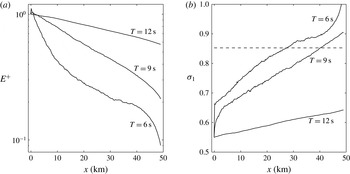
(a) Ensemble average of the forward propagating wave energy
 $E^{+}$
and (b) the directional spread
 ${\it\sigma}_{1}$
through
 ${\approx}50~\text{km}$
of simulated MIZ, for
 $T=6$
,
 $9$
and
 $12~\text{s}$
. In (b) the dashed line corresponds to the theoretical value of
 ${\it\sigma}_{1}$
characterizing an isotropic directional wave field. This value is independent of the wave period.

Figure 6(a) shows the average wave energy profile
 $E^{+}(x)$
across the simulated MIZ for
 $T=6$
,
 $9$
and
 $12~\text{s}$
. We observe a clear exponential decay of wave energy for
 $T=9$
and
 $12~\text{s}$
. For
 $T=6~\text{s}$
, the wave energy profile is more complicated with three observable regimes: (i) a rapid quasiexponential attenuation for
 $x<10~\text{km}$
; (ii) a slower quasiexponential attenuation for
 $10\,\text{km}<x<40\,\text{km}$
; and (iii) an acceleration of the decay for
 $x>40~\text{km}$
. Numerical simulations (not displayed here) showed that the transition between the first and second regimes arises because of the limited extent of the array in the
 $y$
-direction. Specifically, the two regimes merge into a single attenuation regime as
 $L_{y}$
increases, with an attenuation rate between those of the first and second regimes. This situation is difficult to achieve, however, as it is positively correlated to the extent of the MIZ in the
 $x$
-direction. Acceleration of the wave energy attenuation for
 $x>40~\text{km}$
is observed for the three wave periods considered here, although the effect becomes weaker as the wave period increases. As discussed earlier, the existence of this regime may be explained by the lack of backscattered waves near the end of the array, which in turn reduces the forward propagating wave energy (due to reflection from these backscattered components in this region).
To quantify the spreading experienced by the wave field through the MIZ, we use the so-called directional spread
 $$\begin{eqnarray}{\it\sigma}_{1}({\it\xi}_{q})=\sqrt{2(1-r_{1}({\it\xi}_{q}))}\quad (q=0,\ldots ,S),\end{eqnarray}$$
where
 $$\begin{eqnarray}r_{1}({\it\xi}_{q})=\left(\left(\int _{-{\rm\pi}/2}^{{\rm\pi}/2}\cos ({\it\chi})\tilde{S}_{q}^{+}({\it\chi})\,\text{d}{\it\chi}\right)^{2}+\left(\int _{-{\rm\pi}/2}^{{\rm\pi}/2}\sin ({\it\chi})\tilde{S}_{q}^{+}({\it\chi})\,\text{d}{\it\chi}\right)^{2}\right)^{1/2},\end{eqnarray}$$
with
 $\tilde{S}_{q}^{+}({\it\chi})=S_{q}^{+}({\it\chi})/E^{+}({\it\xi}_{q})$
the normalized forward energy density at
 $x={\it\xi}_{q}$
.
Our definition for
 ${\it\sigma}_{1}$
is the forward-only spectrum version of the standard definition, in which the integrals in (6.3) range from
 $-{\rm\pi}$
to
 ${\rm\pi}$
to account for the full directional range (see Krogstad Reference Krogstad, Hauser, Kahma, Krogstad, Lehner, Monbaliu and Wyatt2005, (2.16)). The original definition of
 ${\it\sigma}_{1}$
is the standard deviation of a random variable with periodic probability density function, in this case the energy spreading function
 $D({\it\tau})$
defined in (5.2). For forward propagating waves,
 $D({\it\tau})$
is then simply replaced by
 $\tilde{S}_{q}^{+}({\it\chi})$
.
The directional spread is plotted in figure 6(b) across the simulated MIZ, for
 $T=6$
,
 $9$
and
 $12~\text{s}$
. We observe a jump in
 ${\it\sigma}_{1}$
for
 $T=6$
and 9 s as the cosine-squared directional wave field enters the MIZ, indicating a positive correlation between the amount of scattering and directional spreading. After the initial jump, the directional spread increases linearly with
 $x$
for these two wave periods. For
 $T=12~\text{s}$
,
 ${\it\sigma}_{1}$
increases at a linear rate from the start of the array. To the best of the authors’ knowledge, the constant rate of directional spreading (according to the
 ${\it\sigma}_{1}$
measure) within the random array has not been previously observed or simulated.
The theoretical value of
 ${\it\sigma}_{1}$
for an isotropic field is denoted by
 ${\it\sigma}_{1}^{(iso)}$
. It is calculated by setting
 $\tilde{S}_{q}^{+}({\it\chi})=1/{\rm\pi}$
in (6.3) (so it integrates to 1), which gives
 ${\it\sigma}_{1}^{(iso)}=\sqrt{2(1-2/{\rm\pi})}\approx 0.8525$
. This value is indicated by a dashed horizontal line in figure 6(b). It is seen that, for
 $T=6$
and 9 s,
 ${\it\sigma}_{1}$
increases beyond that line, suggesting that the directional spectrum becomes distorted after reaching its isotropic state. To interpret the behaviour of these curves, we analyse the directional spectrum at different locations in the array.
Ensemble average of the normalized forward energy density function
 $\tilde{S}_{q}^{+}({\it\chi})$
for
 $T=6~\text{s}$
(a,c,e,g,i) and 9 s (b,d,f,h,j). The energy densities are plotted for (a,b)
 $q=45$
(i.e.
 $x\approx 10~\text{km}$
), (c,d)
 $q=89$
(i.e.
 $x\approx 20~\text{km}$
), (e,f)
 $q=133$
(i.e.
 $x\approx 30~\text{km}$
), (g,h)
 $q=177$
(i.e.
 $x\approx 40~\text{km}$
) and (i,j)
 $q=221$
(i.e.
 $x\approx 50~\text{km}$
).

Figure 7 shows the normalized forward energy density
 $\tilde{S}_{q}^{+}({\it\chi})$
for
 $q=45,89,133,177$
and 221, corresponding to
 $x\approx 10,\,20,\,30,\,40$
and 50 km respectively. Panels (a,c,e,g,i) and (b,d,f,h,j) show the evolution of the energy density (running from (a,b) to (i,j)) through the array for
 $T=6$
s and 9 s respectively. The curves are generated by averaging over the 10 realizations of the array and smoothing (using a moving average). We observe a gradual spreading of the densities towards isotropy for both wave periods, as the most energetic incident wave components (at the small- to midrange angles
 $|2{\it\chi}/{\rm\pi}|\lessapprox 0.8$
) attenuate while the lower-energy components (at large angle) grow slightly. After reaching a quasi-isotropic state, the wave energy at the midrange angles keeps decreasing, while large-angle components keep growing, which explains the values of
 ${\it\sigma}_{1}$
larger than
 ${\it\sigma}_{1}^{(iso)}$
in figure 6(b). Numerical tests (not displayed here) have shown that this behaviour originates from the limited extent of the array in the
 $x$
-direction; extending the array in the
 $x$
-direction, we observe the same linear growth of
 ${\it\sigma}_{1}$
until
 ${\it\sigma}_{1}^{(iso)}$
is reached, at which point the directional spread remains quasiconstant before it begins to grow again near the end of the array. We conjecture that the acceleration of the energy decay near the end of the array, as observed in figure 6(a), affects the midrange angles more than the large angle components, resulting in the distorted energy densities seen in figure 7(i,j).
6.1. Attenuation coefficient
The key quantity of existing wave attenuation models in the MIZ is the attenuation coefficient, which defines the rate of exponential attenuation of wave energy in an ice-covered sea. At present, this is the only quantity used to parameterize wave–sea-ice interactions in large-scale IOMs (e.g. Williams et al. (Reference Williams, Bennetts, Squire, Dumont and Bertino2013a ,Reference Williams, Bennetts, Squire, Dumont and Bertino b ) using the scattering/viscous model of Bennetts & Squire (Reference Bennetts and Squire2012b )) and SWMs (Rogers & Orzech (Reference Rogers and Orzech2013) using the viscous models of Liu, Holt & Vachon (Reference Liu, Holt and Vachon1991a ) and Wang & Shen (Reference Wang and Shen2010)).
To extract the attenuation coefficient from our simulations, we fit an exponential curve to the computed data
 $E^{+}({\it\xi}_{q})$
,
 $q=0,\ldots ,220$
, i.e.
 $$\begin{eqnarray}E^{+}(x)\approx E^{+}(0)\text{e}^{-ax},\end{eqnarray}$$
where
 $a$
is the attenuation coefficient of wave energy and
 $E^{+}(0)=\exp (a{\it\xi}_{0})$
. We then use linear least-square regression to estimate the expected value
 $\overline{a}(T)$
for each wave period
 $T$
(with the overbar denoting the expected value of a random variable). Our approach is similar to experimental measurements, in which the attenuation coefficient is extracted from the actual wave energy profile through a realization of the MIZ.
For each estimated
 $\overline{a}$
value, we compute the standard error that accounts for the goodness of the least-square fit and the variability of the ensemble averaging process. The statistical method used to estimate the standard error is based on the random effects model and the maximum likelihood method. It is described by Brockwell & Gordon (Reference Brockwell and Gordon2001) in the context of medical science.
Wave energy attenuation coefficient
 $\overline{a}$
as a function of wave period
 $T$
in the range 6–15 s. The error bars represent the standard error of each estimated value of
 $\overline{a}$
, and account for the goodness of the least-square fit and the variability in the ensemble of simulations.

Figure 8 shows the attenuation coefficient as a function of wave period, in the range
 $T=6$
–15 s. It should be noted that the order of magnitude of
 $a$
is
 $O(10^{-6}{-}10^{-5})$
, which is slightly lower than attenuation coefficients estimated from field observations (see, e.g., Wadhams et al. (Reference Wadhams, Squire, Goodman, Cowan and Moore1988), Meylan et al. (Reference Meylan, Bennetts and Kohout2014), observing that our simulations have not been parameterized to match these data sets in regard to the physical moduli involved). This is not surprising as scattering is the only physical process considered here, while in nature other dissipative processes would contribute to the decay of wave energy in the MIZ. The relatively wide incident directional spectrum used for the simulations (i.e. the cosine-squared spreading function) may also contribute to these low values of the attenuation coefficients.
Qualitatively, the dependence of the attenuation coefficient on the wave period is as expected, as
 $\overline{a}$
decreases for increasing
 $T$
. As the wave period becomes smaller, the attenuation coefficient seems to level off. Interestingly, this feature looks similar to the onset of the rollover effect observed in several data sets reported by Wadhams et al. (Reference Wadhams, Squire, Goodman, Cowan and Moore1988). We do not claim, however, that our model is capable of reproducing this effect, which was hypothesized to be a consequence of local wind wave generation, nonlinear wave–wave interactions or dissipative processes, none of which are considered in our model. An extensive sensitivity analysis would be required to interpret this feature in our model, which is beyond the scope of the present case study. We also observe an increase of the attenuation coefficient for
 $T=15~\text{s}$
, which is probably due to the relatively large variability of the attenuation coefficient between individual simulations when the attenuation rate is very small. It should be noted, however, that a similar effect has been reported by Wadhams et al. (Reference Wadhams, Squire, Goodman, Cowan and Moore1988) in their field data, although these authors did not comment on this feature.
6.2. Rate of spreading and distance to isotropy
As observed in figures 6(b) and 7, our model is capable of reproducing the directional spreading experienced by the wave field as it travels through the MIZ. We utilize the apparent linear relationship between
 ${\it\sigma}_{1}$
and
 $x$
observed in figure 6(b) to quantify the directional spreading, by fitting a linear curve to the subset of computed data
 ${\it\sigma}_{1}({\it\xi}_{q})$
,
 $q=q_{\mathit{min}},\ldots ,q_{\mathit{max}}$
. Thus,
 $$\begin{eqnarray}{\it\sigma}_{1}(x)\approx {\it\sigma}_{1}^{0}+sx,\end{eqnarray}$$
where
 $s$
is the (constant) rate of directional spreading,
 ${\it\sigma}_{1}^{0}={\it\sigma}_{1}(0)$
, and the lower and upper bounds,
 $q_{\mathit{min}}$
and
 $q_{\mathit{max}}$
, are determined manually for each
 $T$
. A linear least-square regression is used to estimate
 $\overline{s}(T)$
, as for the attenuation coefficient. The standard errors are also calculated using the statistical method mentioned in § 6.1.
(a) Rate of directional spreading
 $\overline{s}$
as a function of wave period
 $T$
in the range
 $6$
–
 $15$
s. (b) Distance to isotropy
 $\overline{x^{(iso)}}$
plotted over the same range of wave periods. Error bars are computed as in figure 8.

The mean rate of directional spreading,
 $\overline{s}$
, is plotted as a function of wave period in figure 9(a). For
 $T\leqslant 10~\text{s}$
, the rate of spreading only depends weakly on the wave period, with
 $\overline{s}=5{-}6\times 10^{-6}~\text{m}^{-1}$
. The minimum observed at
 $T=8~\text{s}$
and the maximum at
 $T=10~\text{s}$
are difficult to interpret physically, although random variability may be a factor as there are relatively large error bars in this regime. For longer wave periods (
 $T\geqslant 10~\text{s}$
),
 $\overline{s}$
decreases monotonically for increasing wave period, which is sensible as directional spreading is caused by scattering, which diminishes for increasingly long waves.
We now use the more tangible quantity of the distance to isotropy, denoted
 $x^{(iso)}$
, to describe the spreading. We stated earlier that the wave field becomes isotropic when
 ${\it\sigma}_{1}={\it\sigma}_{1}^{(iso)}\approx 0.8525$
, so using (6.5) we can infer the distance from the ice edge to reach isotropy to be
 $$\begin{eqnarray}x^{(iso)}=\frac{{\it\sigma}_{1}^{(iso)}-{\it\sigma}_{1}^{0}}{s}.\end{eqnarray}$$
Care must be taken in estimating
 $x^{(iso)}$
and its variance for each simulation, as
 ${\it\sigma}_{1}^{0}$
and
 $s$
are random variables with an underlying probability distribution, for which we have calculated the expected values and covariance matrix. Equation (6.6) is actually the first-order approximation of the expected value of the ratio distribution. A (better) second-order formula for estimating the expected value of the distance to isotropy is given by
 $$\begin{eqnarray}\overline{x^{(iso)}}\approx \frac{{\it\sigma}_{1}^{(iso)}-\overline{{\it\sigma}_{1}^{0}}}{\overline{s}}-\frac{\text{Cov}({\it\sigma}_{1}^{0},s)}{\overline{s}^{2}}+\frac{\text{Var}(s)({\it\sigma}_{1}^{(iso)}-\overline{{\it\sigma}_{1}^{0}})}{\overline{s}^{3}},\end{eqnarray}$$
where
 $\text{Var}$
and
 $\text{Cov}$
denote the variance and covariance of random variables respectively (see, e.g., Stuart & Ord Reference Stuart and Ord1999). A first-order formula can also be derived for the variance of
 $x^{(iso)}$
, i.e.
 $$\begin{eqnarray}\text{Var}(x^{(iso)})\approx \left(\frac{{\it\sigma}_{1}^{(iso)}-\overline{{\it\sigma}_{1}^{0}}}{\overline{s}}\right)^{2}\left[\frac{\text{Var}(s)}{({\it\sigma}_{1}^{(iso)}-\overline{{\it\sigma}_{1}^{0}})^{2}}-2\frac{\text{Cov}({\it\sigma}_{1}^{0},s)}{({\it\sigma}_{1}^{(iso)}-\overline{{\it\sigma}_{1}^{0}})\overline{s}}+\frac{\text{Var}({\it\sigma}_{1}^{0})}{\overline{s}^{2}}\right].\end{eqnarray}$$
Figure 9(b) depicts the expected value of the distance to isotropy
 $\overline{x^{(iso)}}$
against wave period. The transition between the low-period and high-period regimes is clearly observed here. Isotropy is reached within the first 40 km of the simulated MIZ for
 $T\leqslant 10~\text{s}$
, and
 $\overline{x^{(iso)}}$
varies little with
 $T$
in this regime. On the other hand,
 $\overline{x^{(iso)}}$
increases abruptly for
 $T\geqslant 11~\text{s}$
, where the wave field spreads very slowly towards isotropy. For
 $T>12~\text{s}$
, values of
 $\overline{x^{(iso)}}$
greater than 500 km are computed, suggesting that long waves experience next to no spreading within the extent of a typical MIZ, i.e. over
 $O$
(10–100) km. The transition between the two regimes correlates with the prescribed maximum floe diameter of 200 m, which is the open water wavelength of an 11.3 s wave. This finding suggests that waves longer than the maximum floe size do not experience significant directional spreading in the MIZ, which agrees with the observations of Wadhams et al. (Reference Wadhams, Squire, Ewing and Pascal1986).
7. Conclusion
In this paper we have devised a linear three-dimensional model of ocean wave attenuation and directional spreading in the MIZ, governed by conservative scattering effects alone. The simulated MIZ is composed of a large random array of floating ice floes, modelled as circular thin elastic plates. A random sea state with prescribed directional spreading function defines the wave forcing. The solution to the scattering problem was obtained using an extended version of the slab-clustering method, recently developed by the authors in the context of acoustic wave scattering (see Montiel et al. Reference Montiel, Squire and Bennetts2015a ), which in this case accounts for evanescent vertical modes generated at each floe edge. This allows us to (i) solve the deterministic multiple scattering of directional wave spectra by thousands to tens of thousands of floes for a manageable computation cost, (ii) simulate the propagation of random sea states in randomly generated arrays of ice floes and (iii) track the evolution of the wave field directional properties through the array.
Numerical convergence tests were conducted, with the key findings that
-
(i) evanescent wave modes have little effect on the multiple scattering solution, even for
 $k_{0}a$
as large as
$O(10)$
, and tightly packed arrays, suggesting that the far-field approximation that neglects these modes is valid for a wide range of parameters, and
-
(ii) a small proportion of the complex branches of the directional domain accurately capture wave interactions between slabs.


Ensemble averaging was used to extract the attenuation and directional spreading properties of realistic random sea states through a random array of ice floes that resembled a real MIZ. Randomness was included in the wave forcing, as an incoherent and ergodic directional sea state with a prescribed energy spreading function. Random arrays of ice floes were produced, with floe sizes drawn from an empirical power-law FSD. An analysis of these random features and the ensemble averaging process was conducted to identify potential sources of computational savings. The following was shown.
-
(i) Only a small number, i.e.
$O(1)$
, of unique floe sizes need to be considered in the FSD, thereby reducing the number of single-floe solutions to compute. -
(ii) For each wave period a critical floe size can be defined, such that smaller floes have negligible effect on the scattering properties of an array, suggesting that the smallest floes can be removed from the array. The critical floe size was found to be similar to the open water wavelength. This reduces the number of floes in each slab and, concomitantly, the computational cost of solving the single-slab problem.
-
(iii) Only a small number of unique slabs (
${<}10$
) need to be considered to generate large multiple-slab arrays by taking random permutations of the unique slabs, reducing the number of single-slab solutions to compute. -
(iv) The introduction of randomness in the array and the directional forcing reduces the variability of the solution, so that a small number (e.g. 10) of random realizations of the array and forcing are required to obtain less than 1 % relative standard error on the solution.


The method to extract wave energy attenuation and directional spreading in large random arrays was presented for a
 $50~\text{km}\times 50~\text{km}$
simulated MIZ (composed of 220 slabs). A directional energy density function was defined at each slab boundary to characterize the directional content of wave energy there. The total wave energy was then obtained by integrating the density over the directional range, while the directional spread was defined as the standard deviation of the normalized density interpreted as a probability density function. The profile of wave energy and directional spread were then plotted for a number of wave periods and analysed. The key findings of this analysis are summarized below.
-
(i) Wave energy profiles at midrange and long wave periods showed clear trends of exponential decay, which is consistent with field observations. A more complicated three-regime attenuation profile was observed at the lower end of the range of wave periods, probably due to the limited extent of the array.
-
(ii) The directional spread increases linearly with distance from the ice edge, until it reaches an isotropic state. For short wave periods, the limited extent of the array causes the directional spread to take values higher than that for theoretical isotropy near the end of the simulated MIZ, as the directional energy density becomes distorted.
-
(iii) By fitting an exponential decay model to the wave energy profile at each wave period, we estimated the attenuation coefficient of wave energy, which is the most important quantity parameterizing wave–sea-ice interactions in large-scale operational models. Our estimates were found to be slightly smaller than those obtained from field observations, which is sensible recalling the other mechanisms of wave energy attenuations that are known to exist in MIZs.
-
(iv) By fitting a linear growth model to the directional spread profile, we estimated the rate of directional spreading (slope of the linear model) and the distance from the ice edge to reach isotropy. It was shown that two regimes of spreading exist. For short wave periods, significant spreading is observed, although the amount of spreading experienced varies little with wave period. For long wave periods, the degree of directional spreading diminishes for increasing wave periods. The transition between the two regimes was found to occur when the wavelength becomes larger than the maximum floe size.
Acknowledgements
F.M. and V.A.S. are supported by the United States Office of Naval Research Departmental Research Initiative ‘Sea State and Boundary Layer Physics of the Emerging Arctic Ocean’ (Award number N00014-131-0279), EU FP7 Grant SPA-2013.1.1-06 and the University of Otago. L.G.B. is supported by an Australian Research Council Discovery Early Career Researcher Award (DE13010157), the Australian Antarctic Science Program (Project 4123) and by the University of Adelaide. The authors are grateful to D. Fletcher for helpful statistical mentorship.
Appendix A. Ergodicity of random directional sea states
Jefferys (Reference Jefferys1987) demonstrated that unrealistic standing wave patterns develop when simulating single realizations of the random sea state (5.1). This is due to coherent interference between wave components of the same frequency at different angles, which is referred to as the phase locking phenomenon. This was also shown to be independent from the number of wave directions
 $N_{\mathit{tr}}$
chosen to simulate the sea state. As a consequence, the sea state is not ergodic, which can be verified by expressing the time average of the wave energy as the autocorrelation of the signal (5.1) evaluated at the origin (see Ochi Reference Ochi1998), i.e.
 $$\begin{eqnarray}P=\frac{1}{2}\mathop{\sum }_{i=1}^{N_{\mathit{tr}}}a_{i}^{2}+\frac{1}{2}\mathop{\sum }_{i=1}^{N_{\mathit{tr}}}\mathop{\sum }_{j=1,\,j\neq i}^{N_{\mathit{tr}}}a_{i}a_{j}\cos A_{ij}(x,y),\end{eqnarray}$$
where
 $$\begin{eqnarray}A_{ij}(x,y)=k_{0}(x(\cos {\it\tau}_{j}-\cos {\it\tau}_{i})+y(\sin {\it\tau}_{j}-\sin {\it\tau}_{i}))+{\it\varepsilon}_{j}-{\it\varepsilon}_{i}.\end{eqnarray}$$
The first term in (A 1) corresponds to the target mean energy of the incident spectrum, which we seek to generate uniformly over the domain. The second term contains all interactions between waves travelling at different angles and depends on the space variables, so the wave energy is not uniform and the sea state is not ergodic. The target mean energy can be partially recovered by taking an ensemble average over many random realizations of the sea state (5.1). The wave energy error then decays as the square root of the sample size (a property of ensemble averaging), with the second term in (A 1) averaging out to zero.
In practice, the uniformity of the wave energy in the spatial domain (i.e. the ergodicity condition) can only be approximated by averaging over a sufficient number of realizations. We perform Monte Carlo simulations to analyse the variability of the mean energy (A 1) at the origin. We simulate a monochromatic sea state with period
 $T=9~\text{s}$
and energy spreading function given by (5.2), recalling that no ice cover is present for these simulations. Simulating (5.2) for 1000 realizations of the sea state (5.1) evaluated at
 $(x,y)=(0,0)$
, we find that the 95 % confidence interval for estimating the mean wave energy
 $\bar{P}$
is
 $0.06<\bar{P}<3.7$
, with expected value 1, accounting for the fact that
 $P$
is exponentially distributed (Jefferys Reference Jefferys1987). This shows the significant variability of the mean wave energy on the random variable of the sea state model. The variability can be reduced by averaging over a sample of mean energy estimates. We generate a new distribution of mean energy
 $\bar{P}$
by estimating (A 1) at different locations of the open ocean, where each mean is obtained by averaging over 50 realizations of the sea state. Invoking the central limit theorem, the distribution of
 $\bar{P}$
is normal, with 95 % confidence interval
 $\bar{P}\approx 1\pm 0.28$
. This theoretical result was confirmed by numerical experiments.
We extend the analysis by estimating the error on the mean energy introduced by the ensemble averaging method to approximate ergodicity. Using the 1000 simulated sea states generated earlier, we estimate the relative standard error of the mean energy on a single realization of the sea state to be
 ${\approx}100\,\%$
. On the other hand, the relative standard error of the mean energy estimated by averaging over 50 random realizations of the sea state is reduced to
 ${\approx}14\,\%$
. From the slow convergence property of Monte Carlo simulations, we estimate that it would take approximately 10 000 simulations to further reduce the relative error to 1 %.
Appendix B. Random array generator
We generate the FSD in a given slab using a binning approach, whereby a small number of floe radii (or bins) are considered, henceforth reducing the number of single-floe solutions to compute. The inputs of the procedure are the dimensions of the ice-covered region in the slab, i.e. the width
 $L_{x}$
and breadth
 $L_{y}$
, the number of bins
 $N_{\mathit{b}}$
, the ice concentration
 $c$
, the minimum and maximum floe radii
 $a_{\mathit{min}}$
and
 $a_{\mathit{max}}$
, and the exponent in the power-law distribution
 ${\it\kappa}$
. Given these parameters, we determine the number of floes
 $N_{i}$
with radius
 $a_{i}$
, for
 $1\leqslant i\leqslant N_{\mathit{b}}$
, and randomly position each floe in the slab using a circle packing algorithm. The algorithm is outlined as follows:
-
(1) define uniformly distributed bins
$a_{i}$
,
$1\leqslant i\leqslant N_{\mathit{b}}$
, with
$a_{1}=a_{\mathit{min}}$
and
$a_{N_{\mathit{b}}}=a_{\mathit{max}}$
; -
(2) compute proportionality constants for each bin,
(B 1)
$$\begin{eqnarray}{\it\lambda}_{i}=\frac{\bar{a}_{i+1}^{1-{\it\kappa}}-\bar{a}_{i}^{1-{\it\kappa}}}{a_{\mathit{max}}^{1-{\it\kappa}}-a_{\mathit{min}}^{1-{\it\kappa}}};\end{eqnarray}$$
-
(3) compute the total number of floes in the slab,
(B 2)
$$\begin{eqnarray}N_{f}=\left\lceil \frac{cL_{x}L_{y}}{\displaystyle {\rm\pi}\mathop{\sum }_{i=1}^{N_{\mathit{b}}}{\it\lambda}_{i}a_{i}^{2}}\right\rceil ;\end{eqnarray}$$
-
(4) compute the number of floes in each bin,
(B 3)
$$\begin{eqnarray}N_{i}=\lceil {\it\lambda}_{i}N_{f}\rceil ;\end{eqnarray}$$
-
(5) adjust the ice-covered domain dimensions to obtain the desired ice concentration,
(B 4)
$$\begin{eqnarray}L=\frac{\displaystyle {\rm\pi}\mathop{\sum }_{i=1}^{N_{b}}N_{i}a_{i}^{2}}{cL_{y}};\end{eqnarray}$$
-
(6) position each floe iteratively at random in the ice-covered domain, such that floe/floe boundaries and floe/domain boundaries do not intersect (circle packing algorithm).


In step 2, we have defined
 $\bar{a}_{i}=(a_{i-1}+a_{i})/2$
,
 $2\leqslant i\leqslant N_{\mathit{b}}-1$
, with
 $\bar{a}_{1}=a_{1}$
and
 $\bar{a}_{N_{\mathit{b}}}=a_{N_{\mathit{b}}}$
. In steps 3 and 4,
 $\lceil .\rceil$
denotes the ceiling function, which then introduces a discrepancy in the concentration of ice floes. Step 5 adjusts the width of the domain to generate an FSD with concentration as specified in the inputs. In step 6, floes are positioned in the domain iteratively in decreasing order of size, allowing us to reach higher concentrations.