


1. Introduction
Climate change refers to long-term variations in temperature and precipitation patterns, sea or ocean levels, and other aspects of the Earth system. Measurement and mitigation of the effects of climate change are pressing and difficult challenges for society. This has serious implications for the insurance sector that is affected by increased claims frequency and severity in several different business lines.
According to the Intergovernmental Panel on Climate Change (IPCC), global surface temperatures from 2011 to 2020 were
 $1.1\,{}^\circ \mathrm{C}$
higher than average in the last half of the
 $19^{\text{th}}$
century, with land surface temperatures increasing by
 $1.59\,{}^\circ \mathrm{C}$
(see IPCC 2023, longer report, p. 42). Climate change poses a variety of increased risks, including more frequent and intense extreme weather events, rising sea and ocean levels that threaten coastal areas, water scarcity and droughts, the disruption of ecosystems and the loss of biodiversity, adverse impacts on agriculture and food security, public health risks, significant economic consequences, and displacement and migration of populations.
For insurance companies, any increase in extreme weather events, such as heat waves, windstorms, floods, wildfires, and droughts, which can cause deaths and significant damage, would result in higher insured losses or coverage limits (see Zhou et al., Reference Zhou, Vilar-Zanón, Garrido and Heras-Martınez2024b, for a more extensive survey of the impact of climate change on insurance). Moreover, if historical data are no longer representative due to changes in weather patterns, insurers need to reassess their risk models and to incorporate climate change projections and long-term climate risk assessments into their pricing to accurately determine premiums.
2. Survey of actuarial climate indices
To complete a survey of the different actuarial climate indices developed in several countries, we first review the methodology defined jointly by Canadian and American actuaries to calculate the Actuaries Climate Index
 $^{\mathrm{TM}}$
(ACI).
2.1. The North American actuaries climate index
 $^{\mathrm{TM}}$

At the turn of this century, the World Climate Research Programme proposed several indices to help summarize useful information on climate change (see Peterson et al., Reference Peterson, Folland, Gruza, Hogg, Mokssit and Plummer2001). In 2012, the Climate Index Working Group of the Casualty Actuarial Society (CAS) Climate Change Committee summarized the scientific knowledge on climate change at the time and proposed to develop a composite index termed the Actuaries Climate Change Index to include information from several climate variables; see their report (Solterra Solutions, 2012). A project to create the ACI, jointly developed by the Canadian Institute of Actuaries, the Society of Actuaries, the CAS, and the American Academy of Actuaries, was then proposed by this same working group in 2014 and finally launched in November 2016 (see ACI, 2018).
The ACI combines information from several important climate variables in historical records of the United States and Canada to study climate change in that part of the world. Just as the Consumer Price Index tracks changes in the cost of a standard basket of goods and services over time, the ACI measures climate risks through a basket of extreme climate events and changes in sea or ocean levels. It is intended to provide actuaries, public policy makers, and the general public with a neutral, factual, and useful quantitative climate change index. As a monitoring tool, it can help us learn about climate change and link it to associated insurance risks; see Figure 1 where the ACI shows a significantly increasing trend in recent years.
Once the ACI provided a factual and objective climate risk measure for North America, the need arose to test whether a similar tool could measure the impact of climate change in other parts of the world and whether the change was similar or not. In fact, despite the observed global nature of climate change, different regions and countries can be affected in different ways.
Comparison of the evolution of insured losses (1970–2020) and the Actuaries Climate Index
 $^{\mathrm{TM}}$
(1961–1990 reference period to 2016).
Source: Swiss Re press release, 2020, and the ACI webpage.

Figure 1 Long description
Panel A: A combination of vertical bar and line graph shows insured losses from 1970 to 2020. The vertical axis represents losses in USD billion at 2019 prices, ranging from 0 to 160. The horizontal axis represents years from 1970 to 2020. The bar graph includes three categories: Earthquakes/tsunami (blue), Weather-related (light blue), and Man-made (yellow). A red line represents the 10-year moving average total insured losses. Notable trends include increasing losses over time, with significant peaks around 2005 and 2010. Panel B: A line graph shows the Actuaries Climate Index for Canada and the U.S. from 1961 to 2016. The vertical axis represents reference period standard deviations, ranging from -1.0 to 2.5. The horizontal axis represents years from 1961 to 2016. The graph includes a reference period from 1961 to 1990, marked by a blue arrow. A black line represents the 5-year moving average. Notable trends include an increase in standard deviations post-1990, indicating more extreme climate events.
In the ACI definition, the focus is on extreme weather events rather than averages; extremes have a greater impact on policyholders and their insured goods, as well as on society and the economy. The index is composed of six variables, each representing a monthly time series starting in 1961, based on measurements from the National Oceanic and Atmospheric Administration (NOAA, see Menne et al., Reference Menne, Durre, Korzeniewski, McNeill, Thomas, Yin, Anthony, Ray, Vose, Gleason and Houston2012), GHCNDEX1 (CLIMDEX, see Donat et al., Reference Donat, Alexander, Yang, Durre, Vose and Caesar2013), and the Permanent Service for Mean Sea Level (PSMSL) (2025); see also Holgate et al. (Reference Holgate, Matthews, Woodworth, Rickards, Tamisiea, Bradshaw, Foden, Gordon, Jevrejeva and Pugh2013). More precisely,
 \begin{equation} ACI=\dfrac {1}{6} \cdot (T90_{std}-T10_{std}+P_{std}+D_{std}+W_{std}+S_{std}), \end{equation}
where
 $T90_{std}$
and
 $T10_{std}$
are standardized variables that measure the frequency of extreme high and low temperatures, respectively,
 $P_{std}$
measures the severity of extreme rainfall precipitations,
 $D_{std}$
stands for extreme frequencies of consecutive dry days,
 $W_{std}$
measures the frequency of days with extreme wind power, and
 $S_{std}$
tracks anomalies in monthly sea or ocean level averages (see Appendix A for more details).
2.2. The Australian Actuaries Climate Index (AACI)
To resume our survey, next we look at Curry (Reference Curry2015), who considers extending the application of the ACI formula to the UK and, more generally, to Europe. He reviews the definition and underlying methodology of the ACI to find that it could be applied in these regions without change, although appropriate data for the region would be needed to do so.
In 2018, the Institute of Actuaries of Australia developed its own Australian ACI (AACI), based on the same methodology as the North American ACI, to measure climate change in Australia; see AACI (2018). The AACI is also calibrated to a 0 average, but over a different reference period, 1981–2010. From Figure 2, we see that, as for the ACI, recent seasonal values of the AACI are almost exclusively above average and that the index 5-year moving average (black curve) shows a strong increasing trend since about 2001.

More recently, Nevruz et al. (Reference Nevruz, Atici and Yildirak2022) proposed the application of the ACI in Turkey, adapting it to the local situation in Ankara, to develop an index suitable for this region. They suggested that choosing the best grid data for their ACI was more important than changing how the index is calculated.
Bridging the gap between physical risk and insurance, Pan et al. (Reference Pan, Porth and Li2022) investigated the effectiveness of ACI in predicting crop yields for (re)insurance rate making. They find that the ACI has significant predictive power for crop yields and yield losses and argue that a high-resolution index could benefit the insurance industry.
2.3. The Iberian actuarial climate index (IACI)
Returning to Europe, in collaboration with the Spanish Institute of Actuaries (IAE), a first draft of a Spanish version of the ACI was defined over a shorter and more recent reference period than for the ACI (1975–1995 in general and 1993–2000 for sea levels). Their temperature variables differ (using the average highs and average lows), as well as the composite index formula; see IAE (2026).
Then Zhou et al. (Reference Zhou, Vilar-Zanón, Garrido and Heras-Martınez2023) also used the North American ACI methodology to build an actuarial climate index for the Iberian Peninsula that they call the Iberian Actuarial Climate Index (IACI); see Figure 3 for its seasonal values and 5-year moving averages. Their paper reviews in detail the methodology and data used to obtain the IACI and, with it, measure climate change in the Iberian Peninsula. An Excel book with IACI values for Portugal, Spain, and its provinces is available in open access (see Zhou et al., Reference Zhou, Vilar-Zanón, Garrido and Heras-Martınez2024a).
Seasonal IACI values; 1961–1990 reference period to 2022.
Source: Zhou et al. (Reference Zhou, Vilar-Zanón, Garrido and Heras-Martınez2023)

All these works show the strong recent interest of the insurance sector in this topic, motivating the development of such indices in new regions, together with the need to create a common index for broader regions, e.g., for Europe. The most recent examples are the Italian Actuarial Climate Index (ITACI, see Rogo et al., Reference Rogo, Garrido and Demartis2025, in Figure 4), the South African ACI (SAACI, see Marais & Moutanabbir, Reference Marais and Moutanabbir2025), or the extension of the Turkish ACI at the national level (see Taylan Selamlar, Reference Taylan Selamlar2026).
Seasonal ITACI values; 1961–1990 reference period to 2024.
Source: Rogo et al. (Reference Rogo, Garrido and Demartis2025)

Figure 4 Long description
A line graph showing seasonal climate index values from 1961 to 2024. The horizontal axis represents the years from 1961 to 2024, and the vertical axis represents the index values ranging from -0.5 to 2.0. The graph includes four colored lines representing different seasons: blue for Winter, green for Spring, yellow for Summer, and orange for Autumn. A black line represents the 5-year moving average. The graph shows fluctuations in the index values across different seasons over the years, with a noticeable increase in the index values in recent years.
The rest of the paper is organized as follows: the extension of the North American ACI methodology to French data is presented in Section 3, leading to the French Actuarial Climate Index (FACI). It updates the FACI draft in Garrido et al. (Reference Garrido, Milhaud and Olympio2023, Reference Garrido, Milhaud, Olympio and Popp2024) to include climate data up to the end of 2024 and corrects the calculation of the drought variable, using linear interpolation between annual values, rather than calculating monthly values as in the previous version. This has a very small impact on the FACI values themselves, but makes them more consistent with the North American ACI methodology. Then a comparison of FACI with other existing indices is given in Section 4. Section 5 gives several high-resolution FACI analyses. Finally, Section 6 proposes a possible application of FACI to parametric insurance. Some concluding remarks and future developments wrap up the paper, while additional technical details appear in the Appendices, for interested readers. In particular, Appendix A reviews in detail the methodology of the North American ACI and its components.
3. The French actuarial climate index
Now consider extending the North American ACI
 $^{\mathrm{TM}}$
methodology to the climate data from France. Here, metropolitan France is defined as the land area ranging from 41
 $^\circ$
to 51
 $^\circ$
north latitude and 6
 $^\circ$
east to 10
 $^\circ$
west longitude, excluding Belgium, as well as Luxembourg to the north, Germany to the northeast, Switzerland to the east, Italy and Monaco to the southeast, and Andorra and Spain to the south. Its largest island, Corsica, is also included in the dataset, but not the French overseas territories.
Since we follow the methodology used for the calculation of the North American ACI, all technical details are deferred to Appendix A. Here, we focus on the data itself and the results obtained.
Then Appendix B explains what climate and sea level data were used for France and Corsica to calculate the FACI.
3.1. Illustrative results for FACI and its components
Figure 5 first depicts a global view of FACI, calculated over the period 1961–2024. As can be seen, FACI has increased steadily in recent years. The reference period was chosen to match that of the ACI
 $^{\mathrm{TM}}$
. It would be worthwhile to study the sensitivity of FACI with respect to the chosen reference period. Similarly, maintaining the same 6 components of the North American ACI
 $^{\mathrm{TM}}$
is needed for comparability. However, the definition of these variables could be misaligned with French climate risks, such as the annual maximum consecutive dry days that are interpolated monthly, or wind exceedances based on daily mean wind power, versus gust-driven losses. This is beyond the scope of the current survey and is deferred to future methodological research. We now focus on each of FACI’s components separately, in order to understand better what drives its evolution.
Seasonal FACI values; 1961–1990 reference period.

To calculate the warm and cool temperature components of each grid cell in France, defined in Appendix A in Equations (A.1) and (A.2), respectively, set daytime from 5 to 22 h and nighttime from 22 to 5 h. The standardized anomalies of the temperature components,
 $T90_{std}$
and
 $T10_{std}$
, are from Equations (A.3) and (A.4), and their seasonal values are plotted in Figure 6.
High- and low-temperature components of seasonal FACI.

Seasonal 5-year moving average, temperature standardized anomalies.

The 5-year moving averages of the standardized anomalies calculated for the two temperature components,
 $T90_{std}$
and
 $T10_{std}$
, are plotted in Figure 7, depicting the changes in the frequency of extreme high- and low-temperature events. Regarding the North American ACI, note here the increase in the frequency of extreme warm temperature events (increase in
 $T90_{std}$
) and the decrease in frequency of extreme cold temperature events (decrease in
 $T10_{std}$
), starting just before the reference period end in 1990, causing the difference
 $(T90_{std}$
–
 $T10_{std})$
to grow. The black line represents the 5-year moving average of this difference, which helps to better visualize the main trend. The change in the frequency of extreme warm temperatures is opposite to that of extreme cold temperature events. It indicates that air temperatures are changing towards more extremes in highs and fewer in lows, that is, warmer days overall.
Next, consider Figure 8, which illustrates the standardized anomalies calculated for the precipitation component,
 $P_{std}$
; see (A.5) for the calculation formula. Observe how the 5-year moving average has taken mainly positive values only in the last 15 years. Positive values of standardized anomalies indicate an increase in heavy precipitation events. Recent seasonal averages often exceed 0.5, a value that can be interpreted to mean that the maximum 5-day rainfall has increased by 0.5 standard deviations, relative to the 1961–1990 reference period mean.
Seasonal and 5-year moving average, maximum 5-day rainfall standardized anomalies.

Then Figure 9 plots the
 $D_{std}$
time series of the maximum consecutive dry days; see the definition in (A.7). The 5-year moving averages experienced a peak around the middle of the reference period and have remained below the 0-average since. Coupled with the increase in heavy precipitations observed in Figure 8, these 2 FACI components suggest a shift to an increase in precipitations in France.
Seasonal and 5-year moving average, consecutive dry days standardized anomalies.

Figure 10 shows that there has been a small, not significant change in the frequency of extremely windy days in France after or during the reference period.
Seasonal and 5-year moving average, wind power standardized anomalies.

Finally, Figure 11 shows the seasonal standardized anomalies of the relative ocean and sea levels. France has experienced a sharp increase after the middle of the 1990s. Sea levels increased over time, in a sustained way, and even at a higher rate most recently. Global rises in sea level are mainly due to the contribution of the melting of continental ice sheets, which accounts for about 80% of the observed rise. The other 20%, called the steric component, comes from the increase in the volume of seawater due to increasing temperatures (thermal expansion; see IPCC 2023; Milne et al., Reference Milne, Gehrels, Hughes and Tamisiea2009). In some eastern parts of the Mediterranean Sea, the steric component plays a lesser role due to the compensating effects of thermal expansion and salinity contraction. For example, in Italy, it is influenced by mass-related processes, such as evaporation, precipitation, runoff, and water transport through straits (see Borile et al., Reference Borile, Pinardi, Lyubartsev, Ghani, Navarra, Alessandri, Clementi, Coppini, Mentaschi, Verri, da Costa, Scoccimarro, Misurale, Novellino and Oddo2025). The sharp increase in sea levels measured here for France implies a series of risks for its coastal areas, such as coastal erosion, flooding, and salinization of freshwater resources.
Seasonal and 5-year moving average, sea level standardized anomalies.

5-year moving averages, FACI and its 6 components.

Figure 12 Long description
A line graph with the horizontal axis labeled from 1966 to 2021 and the vertical axis labeled from -1 to 1.5. The graph includes multiple lines representing different standardized anomalies: W std in blue, S std in red, D std in yellow, P std in orange, T 90 std in green, T 10 std in purple, and F A C I in black. Each line shows different trends over the years, with some lines increasing, decreasing, or fluctuating. The F A C I line shows a general upward trend starting around 1991.
It is worth mentioning that Curry (Reference Curry2015) uses a factor
 $f_S$
as the fraction of the number of coastal to total grid points,
 $0\lt f_S \leq 1$
, to adjust the ACI as follows:
 \begin{equation} ACI_{f-adj}=\dfrac {1}{6}\cdot (T90_{std}-T10_{std}+P_{std}+D_{std}+W_{std}+f_SS_{std}). \end{equation}
Taking into account the particular geography of France, we argue that the variable of ocean and sea level
 $S_{std}$
is important for the entire region. Hence, we set
 $f_S=1$
, as in the ACI, and defer to future work the study of estimating
 $f_S$
as in Curry’s extension of the ACI to the UK (for more on this weighted average formulation, see Rogo et al., Reference Rogo, Garrido and Demartis2025).
Not surprisingly, we observed seasonal volatility for some variables, such as wind, drought, and precipitation, versus a certain continuity and an accumulation effect over time for other variables (such as temperature and sea level, after 1990). Figure 12 summarizes these results by showing the 5-year moving FACI seasonal averages, together with its 6 components. Clearly, changes in sea level and temperatures dominate and are driving the increasing trend in FACI, while the other variables, precipitation and wind power, have experienced little change over the study period.
It is also clear from Figure 12 that some components are correlated. For example, consider that the two temperature variables, the highs curve (
 $T90_{std}$
) and the lows curve (
 $T10_{std}$
), form a mirror image of one another around 0; when
 $T90_{std}$
increases,
 $T10_{std}$
decreases by a similar amount. Figure 13 reports the Pearson correlation coefficients between the six FACI components. These are generally weak, except for the frequency of extreme high- and low-temperatures, as mentioned, and, to a lesser extent, precipitations with sea level.
Correlation coefficients, 6 monthly FACI components.

In addition, there is a significant negative correlation between precipitation and drought variables and a lesser positive correlation between precipitation and wind power, as well as an even more moderate correlation between sea level and the frequency of extreme temperatures, positive for high-temperatures and similar, but negative for low-temperatures.
At this stage, it is natural to question the validity of the methodology used to measure the change in these 6 climate variables. Not only in relation to the multicollinearity observed above but also in relation to the use of standardized anomalies for variables that might not be symmetrically distributed around their mean. These issues are discussed in Appendix C, where the distributions of these 6 standardized anomalies are studied in detail. Apart from the question of the possible exclusion of some of the 6 components included in this first version of FACI, it is also natural to consider the possible inclusion of additional important variables (for example, the North American ACI does not include the ocean and sea temperatures, which could be a driver of change in France).
The next section presents an international comparison of FACI with other existing climate indices using the methodology of the North American ACI; that is, the indices defined for the US, Canada, Spain, and Portugal.
4. Index comparisons
We compare the French, Iberian (Spain and Portugal), and North American (US and Canada) indices. The index defined for the Iberian Peninsula (the IACI) is again based on exactly the same methodology as the North American ACI. So, they can be compared directly with the FACI defined here. We do not include the indices for Australia or Italy in this comparison: although they were initially based on the North American ACI methodology, the Australian AACI was revised, keeping only 3 out of the 6 climate variables, making it less comparable to the other indices. Similarly, the Italian ITACI uses a weighted average, making it difficult to compare it with the other ACIs.
Figure 14 combines the graph of the 5-year moving averages of the seasonal ACI and its 6 components for the US with the same graph for Canada, the IACI for Portugal and for Spain (see Zhou et al. (Reference Zhou, Vilar-Zanón, Garrido and Heras-Martınez2023)), and the FACI for France, already shown above in Figure 12.
Seasonal 5-year moving averages of components used in the ACI (green:
 $T90_{std}$
, purple:
 $T10_{std}$
, orange:
 $P_{std}$
, yellow:
 $D_{std}$
, blue:
 $W_{std}$
, red:
 $S_{std}$
, black: ACI). From top left to bottom right: Canada, USA, Portugal, Spain, and France.

Figure 14 Long description
Panel A: The top left graph shows seasonal 5-year moving averages for Canada. The x-axis represents years from 1966 to 2021, and the y-axis represents the value. Multiple colored lines represent different components, with a black line indicating the ACI. Panel B: The top right graph shows the same data for the USA. Panel C: The bottom left graph shows the data for Portugal. Panel D: The bottom right graph shows the data for Spain. Panel E: The bottom center graph shows the data for France. Each graph has a legend indicating the colors for different components: green, purple, orange, yellow, blue, red, and black for ACI. The graphs show trends and patterns in the data over time for each country.
The first observation is that the change in sea level is dominant in all graphs (red curve), except that of Canada. The other 4 countries show very similar increasing trends and a similar onset time, around the mid-1990s. Portugal and Spain experienced the highest increases, with the
 $S_{std}$
anomaly currently at more than 4.5 standard deviations over its 0-mean. Then, in the US, it is currently at a level of around 3.5, and in France, it is close to 2.0. Canada experienced a large cyclical decrease in sea level at the end of the 1990s and has never caught up with the US since. Also note that ocean and sea level changes depend on the coastal region within these countries. For instance, in Alaska the sea level 5-year moving averages have been constantly decreasing since 1961; see the ACI regional graphs.Footnote 1 In addition, it is not clear how the climate of the inland regions is affected by changes in ocean and sea level, since the variable
 $S_{std}$
is not included in these regional ACIs. Hence, it is difficult to draw general conclusions, other than the significance of the change in this variable
 $S_{std}$
since the reference period and the fact that the colder coastal waters of Canada seem to experience a lesser impact than in the other 4 countries.
The next most dominant change, for all graphs, is for the high-temperature component (green curve). The
 $T90_{std}$
anomalies are currently highest in the US and in France, at close to 2.0, and above 1.0 in the other countries, again with greater oscillations in the US and Canada than in the other 3 graphs. Also, as already noted, the low-temperature component
 $T10_{std}$
exhibits essentially a mirror image trend to that of
 $T90_{std}$
, but over negative values. That is, both contribute significantly to the increasing trend in their respective composite indices.
The findings are quite different for the remaining 3 components, i.e. the maximum 5-day precipitation (
 $P_{std}$
), the drought (
 $D_{std}$
), and wind power (
 $W_{std}$
). In the Iberian Peninsula and in France, the 5-year seasonal averages of
 $P_{std}$
and
 $W_{std}$
also exhibit a stationary behavior, with small oscillations around the 0-mean. In other words, they do not contribute as significantly to the increases in IACI or in FACI, which are essentially due to the sea level, plus the high- and low-temperature components. By contrast, North America experienced a significant increase in maximum five-day precipitations (
 $P_{std}$
) after the reference period. Its increasing trend shows some periodicity. With regard to droughts, the land areas of the US and Canada are very large, each region having different dry periods. Overall, the drought component (
 $D_{std}$
) does not show a clear global trend but is slightly smaller after the reference period. In summary, trends in the precipitation (
 $P_{std}$
) and drought (
 $D_{std}$
) components indicate more extreme precipitations in the US and Canada, compared to France and the Iberian Peninsula.
Even if each component contributes differently to the IACI and the FACI, due to heterogeneous geography, their composite indices show similar increasing trends. Moreover, the index values are themselves similar, ranging from -0.5 to 1.5. In recent years, the most striking thing is that all composite indices have reached values close to 1, despite disparate contributions of their components. This indicates that climate change has led to a similar multiple of their local standard deviation increase in the frequency and severity of extreme weather events, in comparison to the 1961–1990 reference period, whether in France, the Iberian Peninsula, or the US and Canada. In summary, the occurrence of extreme climate events is becoming increasingly common in all these regions.
5. High-resolution analyses; per region/season
The goal here is to study the evolution of FACI, as well as its components, at a high-resolution level. This allows a better understanding of what drives climate change in France and to which extent one should focus on some specific regions when designing efficient practical measures at a microlevel.
5.1. FACI per region/season
Figures 15–18 show the evolution of the seasonal FACI over the last 16 years, at a very high-resolution (cell level, with cells at 0.1
 $^\circ$
latitude
 $\times$
0.1
 $^\circ$
longitude). First, consider the evolution of winter FACI seasonal values over the years 2009–2024.
The first thing we note is the evolution of the colors over the years, whatever the season. Red cells tend to be more prevalent, confirming the global increase trend observed for FACI values in previous illustrations.
Second, extreme climate events seem to occur more frequently during spring and summer in most of France (Figure 16). The south of France seems to be more at risk, as compared to the North–East or North–West. The warmest years are identified easily thanks to these maps; for instance, the year 2023 clearly appears to have been particularly warm (especially in the summer and fall seasons), a well-known fact in France (and also in Europe) that FACI confirms.
Winter FACI, 2009–2024.

Spring FACI, 2009–2024.

Figure 16 Long description
Panel A: A heat map for spring 2009 shows the frequency of extreme climate events in France, with a color scale ranging from -2 to 3 sigma. Panel B: A heat map for spring 2010 shows the frequency of extreme climate events in France, with a color scale ranging from -2 to 3 sigma. Panel C: A heat map for spring 2011 shows the frequency of extreme climate events in France, with a color scale ranging from -2 to 3 sigma. Panel D: A heat map for spring 2012 shows the frequency of extreme climate events in France, with a color scale ranging from -2 to 3 sigma. Panel E: A heat map for spring 2013 shows the frequency of extreme climate events in France, with a color scale ranging from -2 to 3 sigma. Panel F: A heat map for spring 2014 shows the frequency of extreme climate events in France, with a color scale ranging from -2 to 3 sigma. Panel G: A heat map for spring 2015 shows the frequency of extreme climate events in France, with a color scale ranging from -2 to 3 sigma. Panel H: A heat map for spring 2016 shows the frequency of extreme climate events in France, with a color scale ranging from -2 to 3 sigma. Panel I: A heat map for spring 2017 shows the frequency of extreme climate events in France, with a color scale ranging from -2 to 3 sigma. Panel J: A heat map for spring 2018 shows the frequency of extreme climate events in France, with a color scale ranging from -2 to 3 sigma. Panel K: A heat map for spring 2019 shows the frequency of extreme climate events in France, with a color scale ranging from -2 to 3 sigma. Panel L: A heat map for spring 2020 shows the frequency of extreme climate events in France, with a color scale ranging from -2 to 3 sigma. Panel M: A heat map for spring 2021 shows the frequency of extreme climate events in France, with a color scale ranging from -2 to 3 sigma. Panel N: A heat map for spring 2022 shows the frequency of extreme climate events in France, with a color scale ranging from -2 to 3 sigma. Panel O: A heat map for spring 2023 shows the frequency of extreme climate events in France, with a color scale ranging from -2 to 3 sigma. Panel P: A heat map for spring 2024 shows the frequency of extreme climate events in France, with a color scale ranging from -2 to 3 sigma.
Summer FACI, 2009–2024.

Autumn FACI, 2009–2024.

Figure 18 Long description
The image contains fifteen heat maps showing the French Actuarial Climate Index (FACI) for autumn from 2009 to 2024. Each heat map represents a specific year, labeled at the top of each panel. The color scale on the right side of each heat map ranges from -2 to 3 sigma, with colors transitioning from blue (lower values) to red (higher values). The x-axis of each heat map represents longitude, ranging from -5 to 10 degrees, and the y-axis represents latitude, ranging from 42 to 50 degrees. The heat maps show the spatial distribution of the FACI values across France for each autumn season. The color intensity and distribution vary across the years, indicating changes in climate indices over time.
In some locations, the index reaches values of approximately 3. At a single-component level, this would mean that the index has increased by an average of 3 standard deviations over the reference period average. For the composite FACI, which combines the six components, the interpretation is not as straightforward; here the standard deviation of the average of 6 possibly correlated components is not 1. It would be equal to
 $1/\sqrt {6}$
if they were independent. Hence, a seasonal index value of 3 is significantly high, as it is a possibly large multiple of
 $1/\sqrt {6}$
. One possibility of giving an interpretation to the scale of FACI values would be to standardize the composite FACI itself rather than its components, but this would not maintain a common basis for comparison with the North American ACI
 $^{TM}$
.
However, note how the evolution of FACI varies between different cells within a region. Each individual grid cell is affected by climate change in a unique way. That means that the impact of climate change is specific to each area. This heterogeneity also implies that the frequency of extreme climate events varies by region. Indicating that vulnerability and/or adaptability to extreme weather conditions can also differ from one cell to another, this means that such a granular study could be of very high added value for the design of agricultural insurance products.
To better separate the contribution of each component to FACI, one could perform similar map analyses for all its components (temperature, precipitation, drought, wind, and sea level). For conciseness, we have chosen to focus on the temperature in this survey, as the latter seems to be the variable that most contributes to FACI. However, the interested reader can access the complete analysis in Appendix C of Garrido et al. (Reference Garrido, Milhaud and Olympio2023) that plots the progress of the variables temperature, precipitation, drought, and wind over the years 2009–2024.
5.2. Seasonal temperatures per region
Focusing on temperature, one needs to distinguish between two different phenomena, corresponding to extremes for warm as well as cold temperatures. Figures 19–26 plot the temperature progress over the years 2009–2024. First, consider the high temperature variable
 $T90_{std}$
. Note how summers produce more frequent high temperatures, at the same time, as less frequent extreme low temperatures (see Figure 21). To a certain extent, the same can be said about winters. The case of springs and falls is similar, even if a bit less pronounced. Whatever the season, these maps clearly confirm the warming trend.
As a result, the highest FACI values were observed in the summer seasons. Significantly, high FACI values were also observed in spring and fall, although much more geographically dispersed. Thanks to these high-resolution maps, it is easy to see that the impact (in terms of FACI values) can be very different even for two close regions (take, for instance, Fall 2014 and Spring 2015), which makes sense considering the topography of France. However, what is striking is that some regions (like the South–East) show almost exclusively red FACI values in recent years, meaning that these regions seem to be the most affected by climate change (according to the selected weather variables).
Winter
 $T90_{std}$
values, 2009–2024.

Spring
 $T90_{std}$
values, 2009–2024.

Figure 20 Long description
Panel A: A heat map for spring 2009 shows varying sigma values across France, with a color scale ranging from -2 to 3. Panel B: The heat map for spring 2010 displays similar variations, with notable changes in certain regions. Panel C: Spring 2011 shows a significant shift in sigma values, with more areas turning red. Panel D: Spring 2012 continues to show diverse sigma values, with a mix of green, yellow, and red regions. Panel E: Spring 2013 exhibits a more uniform distribution of sigma values. Panel F: Spring 2014 shows increased red areas, indicating higher sigma values. Panel G: Spring 2015 has a mix of green, yellow, and red regions. Panel H: Spring 2016 shows a predominance of green and yellow areas. Panel I: Spring 2017 exhibits a significant increase in red areas. Panel J: Spring 2018 shows a similar pattern with more red regions. Panel K: Spring 2019 returns to a mix of green, yellow, and red areas. Panel L: Spring 2020 shows a significant increase in red areas. Panel M: Spring 2021 exhibits a more uniform distribution of sigma values. Panel N: Spring 2022 shows increased red areas. Panel O: Spring 2023 has a mix of green, yellow, and red regions. Panel P: Spring 2024 shows a predominance of red areas, indicating higher sigma values.
Summer
 $T90_{std}$
values, 2009–2024.

Fall
 $T90_{std}$
values, 2009–2024.

Figure 22 Long description
Panel A: A heat map for autumn 2009 shows varying sigma values across France, with a color scale ranging from -2 to 3. Panel B: The heat map for autumn 2010 displays similar sigma values with a notable shift in color distribution. Panel C: Autumn 2011’s heat map indicates higher sigma values in certain regions. Panel D: The heat map for autumn 2012 shows a more uniform distribution of sigma values. Panel E: Autumn 2013’s heat map reveals increased sigma values in specific areas. Panel F: The heat map for autumn 2014 shows a significant concentration of high sigma values. Panel G: Autumn 2015’s heat map indicates a spread of moderate sigma values. Panel H: The heat map for autumn 2016 displays a mix of low and high sigma values. Panel I: Autumn 2017’s heat map shows a more balanced distribution of sigma values. Panel J: The heat map for autumn 2018 indicates higher sigma values in certain regions. Panel K: Autumn 2019’s heat map reveals a significant increase in sigma values. Panel L: The heat map for autumn 2020 shows a widespread high sigma values. Panel M: Autumn 2021’s heat map indicates a return to moderate sigma values. Panel N: The heat map for autumn 2022 displays a significant concentration of high sigma values. Panel O: Autumn 2023’s heat map shows an extreme increase in sigma values across France. Panel P: The heat map for autumn 2024 indicates a slight decrease but still high sigma values in many regions.
Now consider the low temperatures
 $T10_{std}$
. For consistency, we plot
 $-T10_{std}$
instead, so that high values (in red) mean less frequent extreme lows, that is, warmer days.
Winter
 $-T10_{std}$
values, 2009–2024.

Spring
 $-T10_{std}$
values, 2009–2024.

Figure 24 Long description
Panel A: A heat map for spring 2009 shows France with a color gradient indicating values from -2 to 3 sigma. Panel B: A heat map for spring 2010 shows France with a similar color gradient. Panel C: A heat map for spring 2011 shows France with a color gradient indicating values from -2 to 3 sigma. Panel D: A heat map for spring 2012 shows France with a color gradient indicating values from -2 to 3 sigma. Panel E: A heat map for spring 2013 shows France with a color gradient indicating values from -2 to 3 sigma. Panel F: A heat map for spring 2014 shows France with a color gradient indicating values from -2 to 3 sigma. Panel G: A heat map for spring 2015 shows France with a color gradient indicating values from -2 to 3 sigma. Panel H: A heat map for spring 2016 shows France with a color gradient indicating values from -2 to 3 sigma. Panel I: A heat map for spring 2017 shows France with a color gradient indicating values from -2 to 3 sigma. Panel J: A heat map for spring 2018 shows France with a color gradient indicating values from -2 to 3 sigma. Panel K: A heat map for spring 2019 shows France with a color gradient indicating values from -2 to 3 sigma. Panel L: A heat map for spring 2020 shows France with a color gradient indicating values from -2 to 3 sigma. Panel M: A heat map for spring 2021 shows France with a color gradient indicating values from -2 to 3 sigma. Panel N: A heat map for spring 2022 shows France with a color gradient indicating values from -2 to 3 sigma. Panel O: A heat map for spring 2023 shows France with a color gradient indicating values from -2 to 3 sigma. Panel P: A heat map for spring 2024 shows France with a color gradient indicating values from -2 to 3 sigma.
Summer
 $-T10_{std}$
values, 2009–2024.

Fall
 $-T10_{std}$
values, 2009–2024.

Figure 26 Long description
Panel A: A heat map for autumn 2009 shows temperature variations across France with a color scale ranging from blue to red, indicating sigma values from -2 to 3. Panel B: A heat map for autumn 2010 displays temperature variations with a similar color scale. Panel C: A heat map for autumn 2011 shows temperature variations with the same color scale. Panel D: A heat map for autumn 2012 depicts temperature variations with the same color scale. Panel E: A heat map for autumn 2013 shows temperature variations with the same color scale. Panel F: A heat map for autumn 2014 displays temperature variations with the same color scale. Panel G: A heat map for autumn 2015 shows temperature variations with the same color scale. Panel H: A heat map for autumn 2016 depicts temperature variations with the same color scale. Panel I: A heat map for autumn 2017 shows temperature variations with the same color scale. Panel J: A heat map for autumn 2018 displays temperature variations with the same color scale. Panel K: A heat map for autumn 2019 shows temperature variations with the same color scale. Panel L: A heat map for autumn 2020 depicts temperature variations with the same color scale. Panel M: A heat map for autumn 2021 shows temperature variations with the same color scale. Panel N: A heat map for autumn 2022 displays temperature variations with the same color scale. Panel O: A heat map for autumn 2023 shows temperature variations with the same color scale. Panel P: A heat map for autumn 2024 depicts temperature variations with the same color scale.
Looking at the coldest temperatures, the same phenomenon appears. For the winter season, there have been no negative
 $-T10_{std}$
anomalies in recent years. In addition, there are very significant changes in spring, especially in the southern part of the country.
What is observed with temperature drives the evolution of FACI through the years. The possibility of calculating FACI values at a very granular level is what is interesting here. This is key to adapting to local conditions and taking effective microlevel actions.
6. Insurance applications
With the definition of the ACI and its extension to different countries, several applications followed, linking these indices to insurance or financial losses. We already mentioned Pan et al. (Reference Pan, Porth and Li2022) that use the ACI to predict crop yields for (re)insurance rate making. Similarly, Cheung et al. (Reference Cheung, Ip, Tam and Woo2024) analyze the long-term relationship between extreme weather variables in the ACI and agricultural yields, identifying a significant link between sea level rise and crop productivity. More recently, Yavrum et al. (Reference Yavrum, Selcuk-Kestel and Garrido2026) extended the idea of comparing the ACI with weather-based indices to predict crop yields and price weather derivatives, showing for the first time the potential of ACI as a reliable benchmark for pricing weather-related financial instruments. In similar applications to agriculture, Zhou and Vilar-Zanón (Reference Zhou and Vilar-Zanón2024, Reference Zhou and Vilar-Zanón2025) use a provincial version of the IACI to price crop insurance.
Climate risk impacts the insurance sector in general, not only in agriculture. The examples above focus on the first published applications of ACIs, mostly on modeling crop yields and agricultural insurance losses. Before developing an illustrative example of a general application of ACIs, for completeness of this review, we list here some recent publications in the actuarial, statistical, and climate science literature on climate-related claims evidence for property and motor insurance.
The negative impact of climate change on the property and casualty insurance sector (P&C) is highlighted in Moody’s (2018): losses could go far beyond model predictions due to the difficulty in forecasting catastrophic losses and the high correlation of climate-exposed risks. An example of such losses due to extreme drought is given in Heranval et al. (Reference Heranval, Lopez and Thomas2023). The authors use machine learning methods and a standardized soil wetness index to model insured property damages due to clay soil shrinkage (see also the references therein for more examples in P&C insurance). Another recent example is in auto insurance; Fung et al. (Reference Fung, Jeong and Tzougas2025) quantify the risks that weather-related hazards, driven by climate change, pose to the frequency of claims in auto insurance. For the impact on property insurance, see the recent contributions of Gao and Shi (Reference Gao and Shi2025) and Gudmundarson et al. (Reference Gudmundarson, Tzougas and Christopoulos2026), plus the extensive literature review that these works provide.
Other insurance sectors that are affected by climate risks are life and health insurance, pensions, and social security. Often, this effect is not only on insurance liabilities but also on the capitalization and investment sides. Several survey papers study the global impact of some aspects of climate change on mortality and/or morbidity. For example, D’Ippoliti et al. (Reference D’Ippoliti, Michelozzi, Marino, de’Donato, Menne, Katsouyanni, Kirchmayer, Analitis, Medina-Ramón, Paldy, Atkinson, Kovats, Bisanti, Schneider, Lefranc, Iñiguez and Perucci2010) define what constitutes a heat wave and link it to mortality data for nine European cities, while Song et al. (Reference Song, Wang, Hu, Yue, Zhang, Liu, Tian and Shang2017) give a comprehensive survey of studies on the impact of ambient temperature, and Arsad et al. (Reference Arsad, Hod, Ahmad, Ismail, Mohamed, Baharom, Osman, Radi and Tangang2022) and Milhaud and Gouthon (Reference Milhaud and Gouthon2024) look at heat waves, both for mortality and morbidity. Barigou et al. (Reference Barigou, Patten and Zhou2025) model and forecast mortality using the ACI. See also Robben et al. (Reference Robben, Barigou and Kleinow2026), in the actuarial literature, and the references therein. For the impact of climate on the capitalization of insurance companies, see, for instance, Mbarek et al. (Reference Mbarek, Labidi, Dabbous and Nammouri2026), and for optimal asset allocations in a context of climate change, Raynal and Loisel (Reference Raynal and Loisel2026).
Finally, for a more complete survey of research on the impact of climate risk in the insurance sector and on insurance applications of actuarial climate indices, see Zhou et al. (Reference Zhou, Vilar-Zanón, Garrido and Heras-Martınez2024b).
Climate derivatives and parametric insurance contracts are two types of products that can be used to transfer climate risks, apart from event-linked securities. This section focuses on the parametric insurance type of cover. The main advantage of parametric insurance over climate derivatives is its flexibility, while the main disadvantage is its price; climate derivatives are often cheaper, as they trade on a stock market without requiring the work of insurers. By contrast with a classical insurance product, the benefit payoffs of parametric insurance contracts are triggered by the value of a predetermined index when it reaches a fixed threshold.
The application illustrated here uses FACI as the trigger index, based on historical climate data for France. With it, we calculate premiums of parametric insurance covers for losses generated by climate events.
6.1. Foreword on parametric insurance
A parametric insurance, also known as index insurance, has the defining characteristic that its benefit payoff is triggered by a parameter or index value crossing a predetermined threshold, while for a classical insurance, it is the occurrence of an insured loss that triggers the benefit payment.
Current parametric insurances are mostly based on climate variables/indices whose values are easily obtained (sunshine hours, hurricane wind power, and rainfall), for example, information available from meteorological reports. This type of insurance is popular with farmers seeking a harvest income guarantee. However, the idea can be extended to any risk for which the benefit can be based on an existing objective index. The benefit payment process of a parametric insurance is the simplest. Any time the index reaches the predetermined threshold stipulated in the contract, the benefit is due, and the insurer pays a lump sum that depends on how much the index has exceeded the threshold. As such, the indemnity payment can be paid very quickly, without the need for an expert appraisal to evaluate the losses or to force on the insured the burden of proof of the damage incurred. In fact, the indemnity here does not depend on the loss incurred, only on the index value and the predetermined threshold. The idea is that, at least partly, the two concepts should be linked.
Several actuarial research theses examine the use of parametric insurance products and/or climate derivatives. For example, Nguyen and Ritleng (Reference Nguyen and Ritleng2014) study a parametric insurance product for the risk of heavy rainfall in Jamaica, whereas Vendé (Reference Vendé2003) looks at the correlation between different climate indices in the rate making of a parametric cover for catastrophe reinsurance (CatRe). Denizot and Plouhinec (Reference Denizot and Plouhinec2008) evaluate the use of different temperature models in pricing climate derivatives. By contrast, Gilles and Finas (Reference Gilles and Finas2011) consider the management of wind risk for the production of eolic electricity. They propose a solution based on mathematical finance to build appropriate climate derivatives, using purely meteorological indices for nonagricultural applications. Koch (Reference Koch2011) considers the creation of a parametric crop yield insurance product based on a climate index. Leprince (Reference Leprince2001) describes two US crop insurance products, for yield and income, and their use in risk management. Batisse and Mercuzot (Reference Batisse and Mercuzot2009) and Fosso and Seretti (Reference Fosso and Seretti2010) discuss the rate-making process for agricultural crop insurance.
The underlying principle of parametric insurance is the construction of an index correlated with the variable of interest (e.g., sales, crop yields, crop quality, etc.). However, such an index must respect certain properties:
-
1. observable and easily measurable,
-
2. objective,
-
3. independently verifiable,
-
4. regularly communicated within a convenient delay,
-
5. consistent over time.
Such an index does not need to be meteorological. For example, it could be the crop yield of a given region published by an independent authority. What emerges from the literature is that parametric insurance appears to be an adapted solution to manage non-catastrophic climate risk, at least as a complementary coverage in conjunction with other hedging instruments. For a summary of the current parametric insurance market, see Garrido et al. (Reference Garrido, Milhaud, Olympio and Popp2024).
6.2. Parametric insurance market
Descartes Insurance, a highly specialized insurtech company, received in November 2022 the regulator’s certification, the Autorité de contrôle prudentiel et de résolution, awarded sparsely on the French market of parametric or index insurance. This market player specializes in the design of insurance products that automatically pay benefits to large enterprises or countries, when a climatic event or a natural catastrophe, occurs and a predetermined index reaches a certain threshold. In recent years, a niche market has formed around start-ups, such as Descartes but also traditional insurers, such as AXA through its subsidiary AXA Climate, and reinsurers, like Swiss Re or Munich Re, as well as some large brokers.
In October 2022, Eunice Jesang, a Kenyan farmer in Makueni County, subscribed to a crop insurance policy for her corn harvest. Her quotation allowed her to participate in the Lemonade Crypto Climate Coalition, a blockchain-based parametric crop insurance pilot program, an initiative of the Lemonade Foundation. Their objective is to support millions of small farmers in regions of the world where traditional storm insurance is not accessible or is not offered.
The specialized broker Atekka has also developed some index insurance solutions. Launched in Cognac in 2021 with the agricultural cooperative Océalia and the data provider Understory, their parametric insurance program against frost and hailstorms, which affect vineyards, has already sold a dozen contracts. The frost cover for Cognac vineyards has worked well since its inception. Clients know from the contract signature that an indemnity will be paid, for example, 30% of the insured capital, in the case of a trigger if a temperature of
 $-2 {}^\circ \mathrm{C}$
or less is recorded in their vineyards. The parametric solutions of Atekka complement traditional insurance products. For larger winegrowers’ operations, classical multirisk climate insurance contracts are sold with a high deductible of 20 to 25%. Parametric insurance can be used to cover this deductible that would otherwise be charged to the farmer.
Club Med also uses parametric insurance for its Caribbean villages, threatened by hurricanes and earthquakes.
After creating, in February 2021, its practice in parametric insurance, Bessé, a broker from Nantes, joined AXA Climate in 2022 to develop parametric insurance solutions for agricultural subsidiaries.
6.3. Rate making process
The parametric insurance rate-making process is similar to that of classical insurance. The usual desirable properties on premiums apply: (i) the charged premium should be larger than the net premium, (ii) premiums must be an increasing function of potential losses, and (iii) premiums should be sub-additive, in general, and additive for independent risks. As for classical insurance, net premiums are adjusted by a risk loading, following some premium principle, to produce a loaded premium
 $\pi$
. For example:
-
• The net premium principle sets a loading
$\theta$
that does not account for the risk of adverse loss (
$L$
) fluctuations around their expectation,
$\mathbb{E}(L)$
:(6.1)
\begin{equation} \forall L \in \mathcal{L}, \quad \pi (L) = (1+\theta )\mathbb{E}(L), \qquad \theta \gt 0. \end{equation}
-
• The variance principle adds a term to account for fluctuations, but is not sub-additive:
\begin{equation*}\forall L \in \mathcal{L}, \quad \pi (L) = \mathbb{E} (L) + \theta \mathbb{V}(L), \qquad \theta \gt 0.\end{equation*}
-
• The standard deviation principle replaces the variance above by the standard deviation. It is sub-additive:
(6.2)
\begin{equation} \forall L \in \mathcal{L}, \quad \pi (L) = \mathbb{E}(L) + \theta \sqrt {\mathbb{V}(L)}, \qquad \theta \gt 0. \end{equation}


The general rating formula for a basic parametric insurance product uses three variables: the entry point
 $E$
, the exit point
 $X$
, and the marginal value of one index unit, say
 $IU$
. The insurance benefit payoffs are determined by the following formula:
 \begin{equation} B = IU \times \unicode {x1D7D9}_{I\gt E} \times \min \{I-E, X-E\}, \end{equation}
where
 $B$
is the benefit value,
 $\unicode {x1D7D9}$
is an indicator function, and
 $I$
is the index value.
This linear benefit formula is the most common on the market, where the index is positively correlated with the benefit payments. Here, the entry and exit points help determine the part of the risk that is transferred to the insurance company, in a way reminiscent of an excess-of-loss reinsurance contract; see Figure 27 for an illustration using FACI as the index.
Parametric insurance benefit examples.

The first contract parameters to fix are the entry and exit points that trigger the benefit payments. The higher the exit point, the higher the premium charged for the cover. In addition, the more probable the index value is between
 $E$
and
 $X$
, the higher the frequency and the size of the benefit payoffs. Another “parameter” is the benefit calculation method. For example, the entry point
 $E$
can be the first quartile, the median, or any other critical threshold that, if passed, triggers a loss of
 $x$
% of the expected yield (from a public institution, such as the Department of Agriculture for crop insurance). The exit point
 $X$
can be, for example, a multiple of
 $E$
, the third quartile, or a higher percentile. For crop insurance commonly sold in the US, the expected yield is set as the last 5 years’ average crop, to which the maximum and minimum are subtracted (Olympic average). Lastly, the current production value has to be evaluated. It can correspond to future prices on financial markets of insured crops or the farmer’s fixed production costs. In the US, all surface yield insurance products are based on the future prices of the Chicago Board of Trade.
There are different methods for the calculation of the premium itself. The first one is based on historical payoffs data. The objective here is not to model the index but to use the historical empirical distribution of the payoffs it generated. For each year of historical data, the benefit is calculated as if the cover were in place. Then these are averaged over the past years. Here, detrending is very important so that the past losses distribution reflects that of future losses. Particular attention must be paid to the quality, as well as the depth of the historical data available, to avoid overfitting. This method is commonly used to obtain a pure premium. Another approach to calculate the pure premium is to fit a known parametric distribution to the empirical index distribution. In practice, the calculation is often performed via Monte Carlo simulations. This is the method illustrated here, although an alternative estimation is possible through extreme value theory.
To control the profitability of the parametric insurance product, insurers often use economical and performance indicators, such as the loss ratio (observed losses over adjusted premiums charged). Depending on the specific risk, the loss ratio study can go back anywhere from 3 to 10 years. The lower the ratio, below 100%, the more profitable the product. Different historical learning and testing datasets are used for the premium calculation and loss ratio analysis through backtesting.
6.4. Numerical illustration
FACI measures extreme weather events, as compared to the 1961–1990 reference period. For the purpose of this numerical illustration, we use 2000–2014 as a learning period and a lower spatial resolution FACI (typically, the resolution is based on 0.25
 $^\circ$
of latitude
 $\times$
0.25
 $^\circ$
of longitude). The high-resolution data are used for visualizations and microlevel regional analysis. Pretend that a parametric insurance product is then set and priced on January 1, 2015, based on these learning data, providing one-year coverage. The case of seasonal or monthly coverages can also be studied; certainly, they will yield different numerical results, but interpretations and key conclusions should be similar. For detailed illustrations of seasonal or monthly coverage, see Appendix D of Garrido et al. (Reference Garrido, Milhaud and Olympio2023).
Empirical versus theoretical statistics for the distribution beta
 $(\alpha = 8.43,\,\beta = 64.49,\,loc = -0.74,\,scale = 12.91)$

Table 1. Long description
A table comparing empirical and theoretical statistics for the distribution beta. The table has two rows and seven columns. The columns are labeled Min., 25th-percentile, Median, Mean, 75th-percentile, Max., and Std. The row labels are Empirical and Theoretical. Row 1: Empirical, Min. -0.28, 25th-percentile 0.42, Median 0.69, Mean 0.751, 75th-percentile 1.08, Max. 2.4, Std 0.4805. Row 2: Theoretical, Min. -0.74, 25th-percentile -, Median -, Mean 0.752, 75th-percentile -, Max. 12.17, Std 0.4801.
First, a parametric distribution is fitted to the monthly FACI values observed during the 2000–2014 learning period shown in Figure 28. As FACI values show seasonality and a long-term trend, the raw values were properly detrended in the first step. Then, of 17 continuous distributions fitted to the detrended values (among the families of gamma, beta, Cauchy, Weibull, Student, uniform, and generalized extreme value distributions), beta
 $(\alpha = 8.43,\,\beta = 64.49,\,loc = -0.74,\,scale = 12.91)$
yielded the highest
 $p$
-value in the Kolmogorov–Smirnov test. Figure 29 shows the fit of the beta, after transforming it back to a raw natural FACI scale by adding back the trend, and compares it to the histogram of the raw observed FACI values. Table 1 gives the empirical summary statistics of the raw observed FACI, comparing them to their corresponding theoretical values. Recall that there is no closed-form expression for the
 $1^{\text{st}}$
quartile, the
 $3^{\text{rd}}$
quartile, and the median of the general beta distribution, and that its expectation and variance, respectively, equal
 $loc+(scale \times \alpha )/(\alpha +\beta )$
, and
 $(scale^2 \alpha \beta )/((\alpha +\beta )^2(\alpha +\beta +1)).$
Training period within red zone, monthly FACI values.

Beta
 $(\alpha = 8.43,\,\beta = 64.49,\,loc = -0.74,\,scale = 12.91)$
density versus histogram on monthly FACI.

This fitted beta distribution is then used to price a one-year insurance coverage. Two parametric insurance coverages are illustrated, for benefits based on (i) the entry point being the median
 $E=0.75$
and the exit point the 75% percentile
 $X=1.08$
, and (ii) an entry point being the mean
 $E=0.963$
and the exit point the 90% percentile
 $X=1.376$
, as in Figure 27. These values are on the natural FACI scale, once trend effects have been added back.
To do so, the beta distribution fitted to detrended FACI values from the 2000 to 2014 learning period is used to generate a sample of 5,000 Monte Carlo simulated monthly FACI iid (detrended) variates. and tested for 2015. Table B.2 reports the summary statistics (mean, median, and other percentiles) for these detrended simulated values; see also Figure 30.
Note that here it is implicitly assumed that once detrended, FACI values are iid over time. The autocorrelation (ACF) tests performed on the simulated detrended data did not show that significant values passed the first lag (one month), remaining within
 $\pm 0.2$
, the ACF being even lower for the squared series.
Annual coverage premiums (
 $X(\%)$
in percent,
 $\theta = 3\%$
, Std = standard deviation, prem. = premium)

Table 2. Long description
A table with 6 rows and 10 columns comparing estimated benefit payoffs for different parameters and scenarios. The columns are labeled as follows: Parameters, E value, X percent, Actual value, Actual payoff, Pure prem. by (a), Pure prem. by (b), mean, Std, median, and min-max. The table presents data for three different medians and three different means, each with varying values for E, X percent, Actual value, Actual payoff, Pure prem. by (a), Pure prem. by (b), mean, Std, median, and min-max. For example, the first row shows med. -0.062, 75 percent, 0.331 value, 279.36 actual payoff, 175.28 pure prem. by (a), 171.92 pure prem. by (b), 170.18 mean, 57.86 Std, 168.76 median, and 0-370.46 min-max.
Simulated monthly FACI values.

Two premium principles (P.P.) are illustrated: (a) denotes the loaded pure premium in (6.1), and (b) represents the standard deviation principle in (6.2). Table 2 reports the entry and exit points on the detrended scale of the simulated FACI values and the estimated parametric insurance benefit payoffs for these two premium formulas, comparing them with the simulated payoffs of an annual coverage in 2015, with a premium loading
 $\theta = 3\%$
. For example, take the first line of Table 2 and apply Equations (6.1), (6.2), and (6.3) to find payoff and pure premiums
 $\pi (L)$
,
 $B$
Note that the actual payoffs exceed not only the mean or median estimated payoffs but are generally close to the maximum of their range of simulated values. In addition, with small loadings, such as
 $3\%$
, both the loaded pure premiums (a) and those based on a loading using the standard deviation (b) would have been insufficient to cover payoffs. Hence, the first conclusion is that to be solvent, an annual parametric insurance coverage with benefit payoffs based on FACI requires risk loadings larger than
 $3\%$
.
Also, in many cases, it makes more practical sense to design and sell parametric insurance based on a climate index for seasonal coverage only, rather than on an annual basis. In such a case, actual payoffs should be more in line with their estimated mean or median values. Furthermore, loaded premiums should be adequate for all loadings, even the smaller ones, and for all premium loading formulas. In general, for a parametric insurance coverage defined on a climate index with seasonal variations like FACI, it is likely that selling a seasonal coverage (e.g., for the summer only) rather than an annual one would be more adequate to reduce the high payoff variations due to seasonal fluctuations of the index.
A final note to mention that parametric insurance is subject to basis risk when there is a mismatch between the insurance payout and the actual losses of the policyholder. For instance, in agricultural parametric insurance, the source of basis risk can be threefold: 1. geographical, if there is heterogeneity in climate conditions at a finer resolution than that of the index. Then the losses of the policyholder may be caused by climate conditions different from those described by the index value. 2. product design, when the definition of the index is imperfect as a loss predictor. For example, an index that includes temperature measurements but not humidity. 3. temporal, when the time period used to design the index does not correspond to the sensitive growing stages of the crop.
Future research shall reveal how correlated FACI is with insured losses in France and in what lines of business basis risk could be a concern. However, this analysis falls out of the scope of this survey paper.
7. Conclusions
This paper reviews the development of actuarial climate indices, starting with the original North American ACI, up to the most recently published one for Italy. Then the same ACI methodology is applied to climate data from France in order to calculate the FACI. After reviewing the methodology and the data used to obtain FACI, with it we study climate change in France since the 1961–1990 reference period, including high-resolution analyses, per component, per season, and per region. Together with the recent indices calculated for Spain, Portugal, and Italy, this FACI represents one more step toward the definition of a European index. In order to help this development, R and Python packages have been developed to gather and streamline all the computational steps needed for these actuarial climate indices; see Zhou (Reference Zhou2025) for the R library to compute the Iberian IACI, and see Milhaud (Reference Milhaud2024a, Reference Milhaud2024b) for the Python and R libraries, respectively, used to compute the French FACI.
As an illustrative application of FACI, the paper concludes with the definition and pricing of a parametric insurance product that could be based on FACI. Two different benefit payoff formulas are illustrated as well as different premium loadings. Annual and seasonal coverages are defined; the simulation study illustrates the better adequacy of premiums for seasonal coverages when the parametric insurance is based on an index, like FACI, that is subject to seasonal variations.
As acknowledged in Appendix C below, the current standardization method for climate variables is not ideal for skewed component distributions. This is a caveat that should constitute a methodological direction for future work.
Supplementary material
The supplementary material for this article can be found at https://doi.org/10.1017/S1748499526100414.
Acknowledgements
The authors thank the Editor, Associate Editor, and two anonymous referees for their detailed and constructive comments that helped improve the manuscript. In addition, they gratefully acknowledge the leadership and financial support of the Chaire d’Excellence Digital Insurance And Long term risk - DIALog.Footnote 2
Data availability statement
The climate data used in this study are openly available in the Copernicus Climate Change Service Climate Data Store (CDS), more specifically in the ERA5– Land hourly data from 1950 to present,Footnote 3 while the sea–level data can be found with Permanent Service for Mean Sea Level (PSMSL) Tide gauge data.Footnote 4 Finally, the code used is available also on Github as a Python Footnote 5 and on CRAN as an R library.Footnote 6
Appendix A. The North American actuaries climate index
$^{\mathrm{TM}}$
(ACI)

Since the methodology of the Actuaries Climate Index
 $^{\mathrm{TM}}$
(ACI) has been used to define the other indices surveyed here, including our French index, for completeness, this section reviews the ACI methodology and its main results; see ACI (2019) for more details.
The ACI was defined originally for the United States and Canada and jointly produced by several actuarial societies in North America. It combines six climate variables; see Table A.1, each being a monthly time series beginning in 1961.
Definition of the ACI components

Table A.1. Long description
A table with three columns and six rows. The columns are labeled Components, Notation, and Definition. The rows are as follows: Row 1: Components, Warm temp., Cool temp., Precipitation, Drought, Wind speed, Sea level. Row 2: Notation, T90, T10, P, D, W, S. Row 3: Definition, Frequency of temp. > 90th percentile, Frequency of temp. < 10th percentile, Max. rainfall/month in 5 consecutive days, Annual max. consecutive dry days, Frequency of wind speed > 90th percentile, Change in sea level.
The ACI uses a reference period from 1961 to 1990 as the basis to measure climate change. The data from this period produce the means and standard deviations used to standardize anomalies for each component, relative to 1961–1990. A monthly standardized anomaly is given by the difference between the given month’s value and the corresponding month’s average over the reference period, then dividing by its standard deviation over the reference period, like a Z–score. “These indices have been generally chosen for their robust statistical properties and their applicability across a wide range of climates” (see Stocker et al., Reference Stocker, Qin, Plattner, Tignor, Allen, Boschung, Nauels, Xia, Bex and Midgley2013, p. 221). Figure 1 plots the seasonal ACI values plus their 5–year moving averages, from 1961 to 2016.
The ACI is calculated monthly, as well as on a seasonal basis. The latter is determined by taking meteorological seasonal averages; for example, the winter average is based on the calendar months of December, January, and February. Then the seasonal standardization is just as for the monthly index.
A.1. Temperature components, T90 and T10
The two temperature components are defined as the frequency of temperatures above the
 $90^{th}$
percentile and below the
 $10^{th}$
percentile, relative to the data from the reference period of 1961 to 1990; see details in Table A.2.
Explanation of temperature indices

Table A.2. Long description
A table with two columns and four rows. The columns are labeled Notation and Explanation. Row 1: Notation, T X 90; Explanation, Percentage of days when daily max. temperature is above the 90th percentile of the reference period distribution for the relevant days. Row 2: Notation, T X 10; Explanation, Percentage of days when daily max. temperature is below the 10th percentile of the reference period distribution for the relevant days. Row 3: Notation, T N 90; Explanation, Percentage of days when daily min. temperature is above the 90th percentile of the reference period distribution for the relevant days. Row 4: Notation, T N 10; Explanation, Percentage of days when daily min. temperature is below the 10th percentile of the reference period distribution for the relevant days.
Because warmer days and warmer nights tend to occur together, the ACI measures the average percentage of days when daytime high temperatures and nighttime high temperatures are greater than the corresponding
 $90^{th}$
percentile, for the base period 1961–1990:
 \begin{equation} T90(j,k)=\dfrac {1}{2} [TX90(j,k)+TN90(j,k)], \end{equation}
where
 $j = Jan, Feb, \ldots , Dec$
and
 $k= 1961,1962, \ldots , 2022$
.
The low temperature measure is calculated using a process similar to that used to calculate the frequency below the
 $10^{th}$
percentile:
 \begin{equation} T10(j,k)=\dfrac {1}{2} [TX10(j,k)+TN10(j,k)], \end{equation}
where
 $j = Jan, Feb, \ldots , Dec$
and
 $k= 1961,1962, \ldots , 2022$
.
The standardized anomalies for high temperatures are calculated as the difference between the monthly frequency of warm temperatures
 $\gt 90$
-percentile and the average monthly frequency of warm temperature during the reference period, divided by the standard deviation over the reference period. The warm temperature
 $T90$
and the cool temperature
 $T10$
use the same algorithm:
 \begin{equation} T90_{std}\ (j,k)=\dfrac {T90(j,k)-\mu _{ref}T90(j)}{\sigma _{ref}T90(j)}, \end{equation}
where
 $j = Jan, Feb, \ldots , Dec$
and
 $k= 1961,1962, \ldots , 2022$
, and
 $\mu _{ref}T90(j)$
is the average monthly frequency of warm temperature for all months during the reference period, while
 $\sigma _{ref}T90(j)$
is the standard deviation of the warm temperatures during the reference period.
The standardized anomalies calculation method for the cold temperatures is consistent with that for warm temperatures.
 \begin{equation} T10_{std}\ (j,k)=\dfrac {T10(j,k)-\mu _{ref}T10(j)}{\sigma _{ref}T10(j)}, \end{equation}
where
 $j = Jan, Feb, \ldots , Dec$
, and
 $k= 1961,1962, \ldots , 2022$
.
As the climate warms up, the occurrence of extreme cool temperatures decreases, and the temperature distribution shifts to the right. Hence, the sign of
 $T10_{std}$
is reversed in the calculation of the ACI to correctly reflect the risk (increasing the ACI when
 $T10_{std}$
decreases to further negative values).
Fewer extreme cold events indicate that the climate is changing, affecting plant and animal ecology and weather patterns. Increased melting of permafrost, increased infectious diseases transmission, and populations of pests and insects that were previously less likely to survive cooler temperatures are all thought to be associated with a reduction in the frequency of extreme cold events.
A.2. Precipitation component, P
The precipitation component focuses on extreme rainfall rather than average precipitation, using the maximum rainfall in any 5 consecutive days within a month, notated as
 $Rx5day(j,k)$
. The percentage anomaly of maximum 5-day rainfall in a month, relative to the reference period value for a given month, is given by:
 \begin{equation} P_{std}\ (j,k)=\dfrac {Rx5day(j,k)-\mu _{ref}Rx5day(j)}{\sigma _{ref}Rx5day(j)}, \end{equation}
where,
 $ j = Jan, Feb, \ldots , Dec$
and
 $ k= 1961,1962, \ldots , 2022$
, while
 $\mu _{ref}Rx5day(j)$
is the average of all months during the reference period, and
 $\sigma _{ref}Rx5day(j)$
is the standard deviation during the reference period.
A.3. Drought component, D
Droughts are measured by the maximum number of consecutive dry days in each year, when the precipitation is less than 1 millimeter (denoted
 $CDD(k)$
). Monthly values are obtained by linear interpolation of annual values:
 \begin{equation} CDD(j,k)= \begin{cases} \dfrac {12-j}{12}CDD(k-1)+\dfrac {j}{12}CDD(k)&j=1,2, \ldots , 11,\\ CDD(k)&j=12. \end{cases} \end{equation}
The standardized anomaly calculations of CDD are similar to those for
 $Rx5day$
:
 \begin{equation} D_{std}\ (j,k)=\dfrac {CDD(j,k)-\mu _{ref}CDD(j)}{\sigma _{ref}CDD(j)}. \end{equation}
A.4. Wind speed component, W
Daily wind speed measurements are converted to wind power,
 $WP$
, using the relationship
 $WP(i,j)=1/2\rho w^3$
, where
 $w$
is the daily mean wind speed and
 $\rho$
is the air density (taken to be constant at
 $1.23 kg/m^3$
). Wind power is used because the destructive potential of wind is better explained by wind power than wind speed. The wind component measures the monthly frequency of daily mean wind power above the
 $90^{th}$
percentile, denoted as
 $WP90$
.
The wind power threshold
 $WP_u(i,j)$
is determined for each day
 $i$
and month
 $j$
in the reference period at each grid point separately. The threshold value is determined as the mean plus 1.28 standard deviations of
 $WP(i,j,k)$
, for all 30 values of the same day and month in the 30-year reference period:
 \begin{equation} WP_u(i,j)=\mu _{ref}WP(i,j)+1.28\cdot \sigma _{ref}WP(i,j). \end{equation}
The day counts when the mean wind exceeds the threshold are then expressed as a percentage of the number of days in the month, providing an exceedance frequency measure, for every month of every year, throughout the entire period:
 \begin{equation} I(i,j,k)=\begin{cases} 1& \mbox{if } WP(i,j,k)\gt WP_u(i,j),\\ 0& \mbox{otherwise}, \end{cases} \end{equation}
 \begin{equation} WP90(j,k)= \dfrac {\sum \limits _{i=1}^{n(j)}I(i,j,k)}{n(j)}, \end{equation}
where
 $i$
represents the day,
 $j$
the month,
 $k$
the year, and
 $n(j)$
the number of days in the month
 $j$
.
Then the standardization is as usual:
 \begin{equation} W_{std}\ (j,k)=\dfrac {WP90(j,k)-\mu _{ref}WP90(j)}{\sigma _{ref}WP(j)}. \end{equation}
A.5. Sea level, S
Monthly mean ocean and sea level measurements are obtained from tide gauges, which record changes in sea level relative to the sea floor (vertical measure, see Table B.2). To avoid negative values, a revised local reference is defined, approximately 7 meters below mean sea level (see Permanent Service for Mean Sea Level (PSMSL) 2025). It is important to note that the height of the land relative to sea level is subject to change due to crustal movements, and these measurements encompass the combined effects of land and ocean positional changes. Standardized anomalies in sea level are calculated using the following equation:
 \begin{equation} S_{std}\ (j,k)=\dfrac {S(j,k)-\mu _{ref}S(j)}{\sigma _{ref}S(j)}. \end{equation}
The use here of a relative sea level variable over that of other available measurements (satellite data, sea surface temperature, etc.) is debatable. To remain as faithful as possible to the North American ACI
 $^{TM}$
methodology, we kept the same definition of their variable
 $S_{std}$
.
A.6. The composite ACI index
The standardized anomalies of the six components above are then combined and averaged to produce the Actuaries Climate Index
 $^{\mathrm{TM}}$
; note that the minimum temperature anomaly
 $T10_{std}$
is subtracted, because the temperature probability distribution curve shifts to the right, as explained earlier:
 \begin{equation} ACI=\dfrac {1}{6}(T90_{std}-T10_{std}+P_{std}+D_{std}+W_{std}+S_{std}). \end{equation}
Figure A.1 plots the 5-year moving averages of this composite ACI, as well as those of its 6 components.
Note the significant increasing trends in the ocean and sea level
 $S_{std}$
and high temperature
 $T90_{std}$
moving averages, as well as in the ACI. Similarly, the low temperature
 $T10_{std}$
averages decrease significantly; given their negative signs, they make an important positive contribution to the ACI.
5-year moving averages, ACI, and its 6 components.
Source: Zhou et al. (Reference Zhou, Vilar-Zanón, Garrido and Heras-Martınez2023, AIAE)

Appendix B. French climate data
We calculate the French Actuarial Climate Index (FACI) with data extracted from the ERA5–Land reanalysis database (see Copernicus Climate Change Service (C3S) Climate Data Store (CDS) 2022).
Instead of using only traditional weather observations from stations or other platforms, the reanalysis data combines weather observations with an advanced computer model, based on the laws of physics, to reconstruct past weather conditions over the entire planet. This is particularly useful in the case of missing weather observations (see, for more information, the reanalysis questions and answers, Copernicus Atmosphere Monitoring Service 2020).
More specifically, the particular climate observations extracted from ERA5–Land here, to correspond to those in Table A.1 and used in the North–American ACI methodology, are: “2m_temperature” to calculate
 $T10$
and
 $T90$
, “total_precipitation” to obtain
 $P$
and
 $D$
, “10m_u_component_of_wind” and “10m_v_component_of_wind” to calculate
 $W$
, and see Table B.1 for more detail.
All these variables are ultimately aggregated to a monthly value but through different processes. For example, temperature variables are extracted on an hourly basis (UTC), then each is split into a nighttime (22 to 5 h) and a daytime value, which serve to determine a minimum and maximum temperature for day and night, and then are converted to the percentage values listed in Table A.2.
Hourly wind speeds are aggregated into a daily average, converted to wind power, and then into a proportion of days that exceed the monthly threshold.
Similarly, total precipitations are extracted hourly and aggregated on a daily basis to define the 2 precipitation components (worst water volume in 5 days per month) and drought (interpolation of the longest period without rain in the year).
Selected ERA5-land dataset variables

Table B.1. Long description
A table with four rows and four columns. The columns are labeled Name, Units, and Description. The rows list climate observation variables: 2m_temperature with units k, total_precipitation with units m, 10m_u-component of wind with units m/s, and 10m_v-component of wind with units m/s. Each row describes the specific climate observation: air temperature at 2m above the surface, accumulated liquid and frozen water, eastward component of the 10m wind, and northward component of the 10m wind respectively.
Source: (Permanent Service for Mean Sea Level (PSMSL), 2025, see Overview).
The sea level variable
 $S_{std}$
was obtained from another source, the Permanent Service for Mean Sea Level (PSMSL) (2025). This database provides monthly mean sea level values for different tide gauge stations. Table B.2 lists all the 40 stations with data available for the coasts of continental France and Corsica that were used to calculate FACI, plus the years of data available at each station. Then a simple average value of these 40 selected stations was used as the
 $S$
variable to calculate FACI. Due to the nature of data collection process, some tidal gauge stations do not have a complete time series of sea level data (see Table B.2 for the percentage of completeness). In such cases, the stations with missing data were not included in the averaging process. For example, if only 25 out of the 40 stations provided data on a particular day, the sea level value for that day was calculated as the average of these 25 stations’ readings. As the missing days are not always for the same stations, varying randomly over the 40 stations, no undue weight is given to any particular station (i.e. robustness of the used averages).
Unlike the ACI for the United States and Canada, which is calculated for 12 sub-regions, the use of high-spatial resolution reanalysis data allows us here to compute FACI over 10,000 cells forming the French grid of 0.1
 $^\circ$
of latitude
 $\times$
0.1
 $^\circ$
of longitude, that is approximately 8 km
 $\times$
11 km = 88 km
 $^2$
(see the NOAA latitude/longitude distance calculatorFootnote 7).
Our high-resolution FACI analyses illustrate the evolution of each grid cell by index component, season, or region, through the years (more on this in Section 5), and show how FACI tracks well the climate change in France over time.
Tide gauge stations, revised local reference (RLR) data

Table B.2. Long description
Panel A: Line graph depicting 5,000 Monte Carlo simulated monthly FACI values. The x-axis represents time in months, and the y-axis represents detrended FACI values. Panel B: Table summarizing the statistical values (mean, median, and percentiles) of the simulated FACI values.
Source: (Permanent Service for Mean Sea Level (PSMSL), 2025, Map–Based Data page).
The first step consists in collecting the original data from the Copernicus Climate websiteFootnote 8 thanks to API requests already implemented within the Python package cdsapi. For each request, the user can play with the dataset name, dates of extraction, GPS coordinates, and weather variables of interest. In practice, since each extraction is limited in size, this task is often performed over small regions that need to be merged in a second step. The output of such a request is a netcdf4-compressed zip file. Then, several data manipulations (for example, using Linux commands) are necessary to create a single file per weather variable over the whole desired territory. Basically, this amounts to concatenating each extracted dataset over the temporal dimension with appropriate merging of time grids and locations. Finally, the user must apply a mask (e.g., the map of France) over the whole rectangular region under study to exclude some points which are not in the region of study due to its irregular shape (not perfectly rectangular). For example, here a reference mask for France was applied,Footnote 9 with a rule to keep the climate data only of those coastal or border cells contained in metropolitan France for at least 80%.
Once all these steps are implemented, one gets as many files as weather variables were selected at the beginning of the process, covering the entire period and country. Going back to Python, it is now possible to exploit these directly, which enables the simple computations required for the actuarial climate index calculations.
To help readers in reproducing these steps to recalculate the FACI values or to obtain an index with the same methodology for another country, Python and R packages are available on GitHub: see Milhaud (Reference Milhaud2024a, Reference Milhaud2024b).
Appendix C. Standardized anomalies
The methodology developed to define the North American ACI is based on the comparison of the standardized anomalies in 6 variables, during and after the 1961–1990 reference period. One might question if centering and standardizing variables, by removing the mean and dividing by the standard deviation, is appropriate for variables that might not be symmetrically distributed around their mean. Especially when these variables measure extremes in the distribution rather than their average.
Figure C.1 plots the histograms of the standardized anomalies for each of the 6 FACI components, in blue for their value during reference period and in red for the anomalies values after 1990.
Histograms of standardized anomalies, before/after 1990.

These histograms vary substantially from one component to another and between months. In general, they are not symmetric about 0, neither before 1990 when that is their mean value nor after 1990. It is better to proceed with the analysis one component at a time.
None of the histograms of the frequency of extreme warm temperature events (
 $T90_{std}$
) are symmetric, and their right skewness is stronger before 1990 than after. What is clear is that the anomalies have reached much larger positive values since 1990. The conclusions are similar for the frequency of extreme cold temperature events (
 $T10_{std}$
), except that the skewness here is to the left and so is the range extension, reaching more negative values since 1990.
With regard to the maximum 5-day precipitation (
 $P_{std}$
) histograms, they vary less than those for temperature, perhaps with the exception of the end-of-the-year months, October, November, and December. Here, the left skewness gets stronger after 1990; that means that the Falls are either getting wetter, or the heavy rains come in later than during the reference period. Couple this with what is observed from the histograms for the maximum number of consecutive days with a precipitation less than 1 millimeter (
 $D_{std}$
). A drastic change in distribution, before and after 1998, occurs in the months of April, showing that it is mainly in the spring that droughts are worse now in France and Corsica than during the reference period.
The mean daily wind power (
 $W_{std}$
) histograms show a much longer right tail for most months, after 1990, in France and Corsica.
Finally, the ocean and sea level variable (
 $S_{std}$
) exhibits the most significant change before and after 1990. The distribution shifts to the right, uniformly, which produces a strong left tail in most months.
In summary, most components of FACI are not symmetrically distributed, especially after 1990. Hence, the standardization used for the North American ACI, subtracting the reference period mean and dividing it by the standard deviation, is not the most appropriate for skewed observations. Alternative methods, based on higher-order moments in the standardization, for instance, like the index of skewness of the kurtosis, or through normalizing variable transformations, could be used. This aspect of the methodology will have to be revisited in future versions of the index for France.

 TM


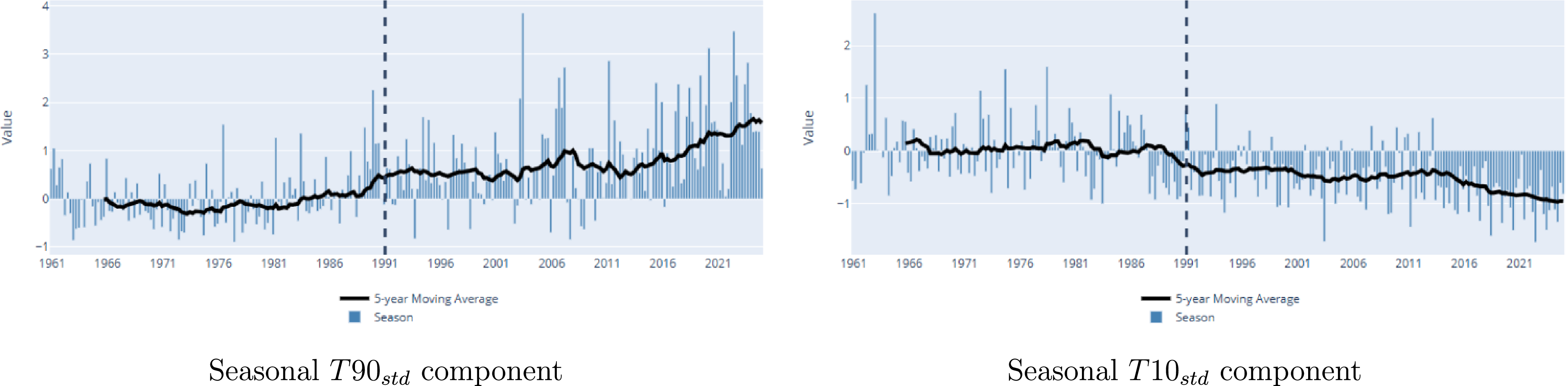


 T90std
 T10std
 Pstd
 Dstd
 Wstd
 Sstd


 T90std

 T90std

 T90std

 T90std

 −T10std

 −T10std

 −T10std

 −T10std
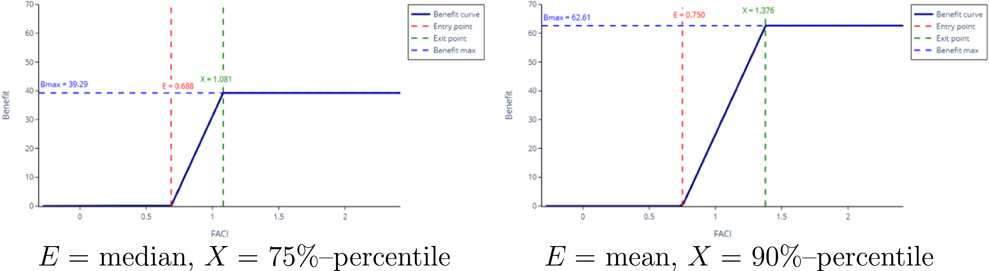

 (α=8.43,β=64.49,loc=−0.74,scale=12.91)


 (α=8.43,β=64.49,loc=−0.74,scale=12.91)
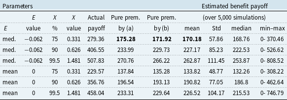
 X(%)
 θ=3%

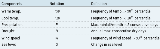
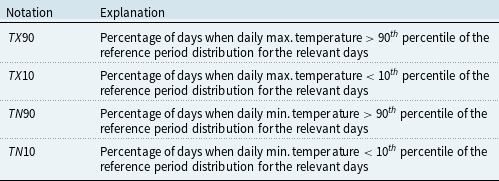

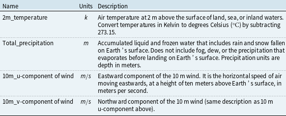
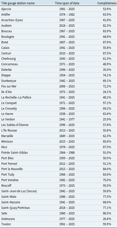


 Open access

