Introduction
Quasi-optical (QO) techniques for characterizing materials in free space are particularly appealing as they allow for permittivity extraction over a wide frequency range and are well-suited for millimeter and sub-millimeter wavelengths, such as those in the W (75–110 GHz) or J (220–330 GHz) bands [Reference García Pérez, Tercero and Lopez Ruiz1, Reference Saenz, L, K, M and VV2] and up to THz frequencies [Reference Hammler, Gallant and Balocco3]. These techniques enable the characterization of materials without specific machining of the sample, which is required when using rectangular or coaxial waveguide cells or cavities [Reference Simakov, Choi, Zuboraj, Carlsten and Choi4, Reference Pantano, Slabbekoorn, Duval and Beyne5]. To allow for precise permittivity extraction, the QO setup must be calibrated so that the actual measured S-parameters are compatible with the model employed in the extraction process (e.g., parallel-sided slab model under plane wave at normal incidence) [Reference Bourreau, Peden and Maguer6]. The plane wave assumption is restricted to a local area where the beam and the material interact, as is the case with a paraxial Gaussian beam, and may lead to an inaccurate model [Reference Mrnka, Appleby and Saenz7].
To evaluate the impact, on the extraction process, of any QO component misalignment during both the calibration and measurement steps or the impairments due to beams with non-planar wavefronts, modeling the test bench can be a valuable approach. Commercial software for full-wave electromagnetic simulation offer interesting capabilities but may be unsuitable for this specific context due to the large component sizes with respect to the wavelengths at these frequencies, leading to excessively long simulation times and a prohibitive memory cost. An intermediate solution involves using proprietary software like Feko, which hybridizes full-wave and asymptotic methods, or GRASP (developped by TICRA), which employs ray launching. However, these software tools do not provide a simple, integrated workflow to model the entire characterization test bench (including antennas and lenses) using a parametric sweep to evaluate the effects of misalignment, misplacement, and other factors on extracted simulated S-parameters. As a result, analyzing how these variables influence accuracy becomes more complex. Analytical models with Gaussian beam incidence can also be implemented to study the interaction with a slab and to extract its permittivity [Reference Mrnka, Appleby and Saenz7].
This paper addresses the modeling of a free-space characterization bench with an in-house tool based on Gaussian beam expansion and tracking. Preliminary results of this work, without the complete modeling of the characterization bench, have been presented at the French Microwave Days conference [Reference Gaudin, Bourreau, Henry and Peden8]. As performed during the experimental characterization, a free-space Thru-Reflect-Line (TRL) calibration such as the one described in [Reference Bourreau and Péden9] is also applied to the simulated S-parameters.
The paper is structured as follows: section “Modeling of quasi-optical systems” outlines the modeling approach; section “Application to a GOLA” provides a comparison between the simulation of a Gaussian optics lens antenna (GOLA) and near-field measurements obtained using a robotic arm; section “Modeling of the characterization bench” presents a simulation of the complete bench including a TRL calibration and a comparison of the results with a dielectric slab model; and finally, section “Conclusion” covers the conclusion and future work.
Modeling of quasi-optical systems
Field expansion
When working with GOLAs, the Gaussian beam formalism [Reference Mrnka, Appleby and Saenz7, Reference Paul10] is a convenient method for propagating the electromagnetic field. However, because the fields produced by some antennas are not purely Gaussian, it becomes practical to expand these fields into a set of Gaussian beams. There are several methods for decomposing a field into Gaussian beams. Instead of describing the radiated field only with the fundamental modes ( $\mathrm{TEM}_{01}$, where TEM stands for transverse electromagnetic) of a Gaussian beam under the paraxial approximation, the field can be expanded into the Gauss–Laguerre modes (for circular aperture shapes), or Gauss–Hermite modes (for rectangular aperture shape) [Reference Paul10, Reference Saleh and Teich11]. However, all those modes share the same propagation axis, implying that the incoming field must exhibit weak divergence. A more suitable solution is to use an expansion surface to decompose the incoming field. A technique introduced in [Reference Chabory, Sokoloff, Bolioli and François Combes12], known as multi-beam expansion, is used to decompose a field into a sum of vectorial Gaussian beams. This method efficiently expresses fields produced by a horn antenna feeding an optical system without requiring a high number of beams [Reference Chabory, Sokoloff and Bolioli13].
Vectorial astigmatic Gaussian beam
The modeling tool relies on the use of Vectorial [Reference Chabory, Sokoloff, Bolioli and François Combes12] Astigmatic [Reference Kochkina, Wanner, Schmelzer, Tröbs and Heinzel14] Gaussian Beams. The electric field from such beams is expressed as
 \begin{equation}
{}^n \boldsymbol{E}_{gb}({}^n \boldsymbol{\rho},z) = \begin{bmatrix}
\boldsymbol{\alpha} \\
-\dfrac{1}{2} \boldsymbol{\alpha}^T\left(\boldsymbol{\mathsf{Q}}(z) + {\textbf{Q}}^\mathrm{T}(z) \right)\boldsymbol{\rho}
\end{bmatrix} u(\boldsymbol{\rho},z),
\end{equation}
with  ${}^n \boldsymbol{E}$ being the electric field written in frame (n),
 $^n \boldsymbol{\rho}$ the transverse coordinates written in frame (n),
 $\boldsymbol{\mathsf{Q}} \in \mathbb{C}^{2\times 2}$ the complex curvature matrix, and
 $\boldsymbol{\alpha} \in \mathbb{C}^{2}$ a couple of transverse polarization coefficients. The longitudinal component is derived from the partial derivatives of the transverse components [Reference Chabory, Sokoloff, Bolioli and François Combes12].
In Eq. 1, u is the scalar function [Reference Chabory, Sokoloff, Bolioli and François Combes12, Reference Kochkina, Wanner, Schmelzer, Tröbs and Heinzel14], defined as
 \begin{equation}
{u}(\boldsymbol{\rho},z) = u_0(z) \exp\left\{-j\dfrac{k}{2}{\boldsymbol{\rho}}^\mathrm{T}\boldsymbol{\mathsf{Q}}(z)\boldsymbol{\rho} + j{\phi}(z) \right\},
\end{equation}
where ρ is the transverse position vector and z is the longitudinal position, both written in the local reference frame (n) of the beam. The normalization factor u 0 ensures that the beam carries 1 W through each cross-sectional area when propagating in a lossless medium.
The definitions of the complex curvature matrix  ${\boldsymbol{\mathsf{Q}}}$, the normalization factor
 $u_0(z)$, and the complex phase
 $\phi(z)$ are provided in Table 1, where k 0 and Z 0 are the wave number and the impedance in free space, respectively.
Gaussian beam expansion
At each sampled point rp on the expansion surface, the incoming electromagnetic field  $\boldsymbol{E}_i(\boldsymbol{r}_p)$ is expanded into a sum of N Gaussian beams, originating from the N sampling points, as follows [Reference Chabory, Sokoloff, Bolioli and François Combes12]:
 \begin{equation}
{}^g \boldsymbol{E}_i(\boldsymbol{r}_p) = \sum_{n=1}^N {}^g\boldsymbol{\mathsf{K}}_n {}^n \boldsymbol{E}_{gb,n}({}^n \boldsymbol{r}_p), ~~ \forall p \in [1, N],
\end{equation}
Components of the Gaussian beam’s scalar function

where  ${}^g\textbf{K}_n \in {\mathbb{R}}^{3\times 3}$ represents the transformation matrix between the local frame (n) of the
 $n$th beam and the reference frame (g) of the system. Each beam
 $\boldsymbol{E}_{gb,n}$ is divided into XZ and YZ polarizations,
 \begin{equation}
{}^n \boldsymbol{E}_{gb,n} = \alpha_{x,n} \cdot {}^n \boldsymbol{E}_{xz,n} + \alpha_{y,n} \cdot {}^n \boldsymbol{E}_{yz,n},
\end{equation}
with  $\alpha_{x,n}$ and
 $\alpha_{y,n}$ being the components of the polarization vector α of the
 $n$th beam, mentioned in Eq. 1. Its propagation axis
 $\hat{\boldsymbol{z}}$ is aligned with the Poynting vector of the incoming field at the corresponding sampled point n.
This leads to a linear system written in its matrix form
 \begin{equation}
\underbrace{\begin{bmatrix}
\boldsymbol{\mathsf{E}}_{xz\cdot x} & \boldsymbol{\mathsf{E}}_{xz\cdot y} \\
\boldsymbol{\mathsf{E}}_{yz\cdot x} & \boldsymbol{\mathsf{E}}_{yz\cdot y}
\end{bmatrix}}_{2N \times 2N} \underbrace{\begin{bmatrix}
\boldsymbol{\mathsf{A}}_x \\
\boldsymbol{\mathsf{A}}_y
\end{bmatrix}}_{2N \times 1} = \underbrace{\begin{bmatrix}
\boldsymbol{\mathsf{E}}_{s\cdot x} \\
\boldsymbol{\mathsf{E}}_{s\cdot y}
\end{bmatrix}}_{2N \times 1},
\end{equation}
where  $\boldsymbol{\mathsf{A}}_x$ and
 $\boldsymbol{\mathsf{A}}_y$ are column vectors filled with the coefficients
 $\alpha_{x, n}$ and
 $\alpha_{y, n}$, respectively, and
 \begin{equation}
\boldsymbol{\mathsf{E}}_{xz\cdot x} = \begin{bmatrix}
\boldsymbol{E}_{xz, 1}(\boldsymbol{r}_1) \cdot \hat{\boldsymbol{x}}_1 & ... &\boldsymbol{E}_{xz, N}(\boldsymbol{r}_1) \cdot \hat{\boldsymbol{x}}_1 \\
\vdots & & \\
\boldsymbol{E}_{xz, 1}(\boldsymbol{r}_N) \cdot \hat{\boldsymbol{x}}_N & ... &\boldsymbol{E}_{xz, N}(\boldsymbol{r}_N) \cdot \hat{\boldsymbol{x}}_N
\end{bmatrix},
\end{equation}
and
 \begin{equation}
\boldsymbol{\mathsf{E}}_{s\cdot x} = \begin{bmatrix}
\boldsymbol{E}_s(\boldsymbol{r}_1) \cdot \hat{\boldsymbol{x}}_1\\
\vdots \\
\boldsymbol{E}_s(\boldsymbol{r}_N) \cdot \hat{\boldsymbol{x}}_N
\end{bmatrix},
\end{equation}
for the XZ polarizations and local axes  $\hat{\boldsymbol{x}}_n$. Note that similar definitions apply to the other terms of Eq. 6. Finally, solving 6 yields the vectors of N polarization coefficients
 $\boldsymbol{\alpha}_x$ and
 $\boldsymbol{\alpha}_y$.
Gaussian beam tracking
The beams generated by the expansion are launched through the QO system. A tracking and bouncing operation is performed to model each beam interaction with the system components. It is assumed that for one incident beam, one reflected and one refracted beams are produced [Reference Chabory, Sokoloff, Bolioli and François Combes12, Reference Kochkina, Wanner, Schmelzer, Tröbs and Heinzel14, Reference Rohani, Ahmad Shishegar and Safavi-Naeini15], each with its own polarization coefficients and curvature matrix.
Computation of the polarization coefficients
Assuming that the incoming beam spot size is small enough with respect to the surface at the intersection point, the polarization coefficients of the reflected and refracted beam can be calculated using the Fresnel formulas [Reference Kochkina, Wanner, Schmelzer, Tröbs and Heinzel14, Reference Rohani, Ahmad Shishegar and Safavi-Naeini15]. The formulas need the polarization coefficients to be expressed in a specific reference frame, where each transverse axis represents either the (S) or (P) polarizations. The S polarization is perpendicular to the incident plane, while the P polarization lies within the incident plane. A transfer matrix is used to express the transverse polarization  ${}^{i}\boldsymbol{\alpha}_I$ of the incoming beam in a new frame, referred to as (sp). The characteristics of this frame, as well as the ones of refracted (t) and reflected (r) beams, are detailed in [Reference Kochkina, Wanner, Schmelzer, Tröbs and Heinzel14]. The Fresnel formulas now apply to calculate the polarization coefficients
 ${}^r \alpha_R$ of the reflected beam and
 ${}^t \alpha_T$ of the refracted beam
 \begin{equation}
{}^{r}\boldsymbol{\alpha}_R = ({}^{sp}\boldsymbol{\mathsf{K}}_{i} {}^{i}\boldsymbol{\alpha}_I) \odot \left[\begin{matrix}
\dfrac{n_i c_2 - n_t c_1}{n_i c_2 + n_t c_1} \\[13pt]
\dfrac{n_i c_1 - n_t c_2}{n_i c_1 + n_t c_2}
\end{matrix}\right]
\end{equation}
 \begin{equation}
{}^{t}\boldsymbol{\alpha}_T = ({}^{sp}\boldsymbol{\mathsf{K}}_{i} {}^{i}\boldsymbol{\alpha}_I) \odot \begin{bmatrix}
\dfrac{2 n_i c_1}{n_i c_2 + n_i c_1} \\[13pt]
\dfrac{2 n_i c_1}{n_t c_1 + n_i c_2}
\end{bmatrix}
\end{equation}

where  $\odot$ is the element-wise product,
 if
 $a\geq 0$, and
 otherwise,
 $\hat{\boldsymbol{n}}$ the normal vector to the surface at the intersection point (oriented toward the incoming medium), ni is the refractive index of the incident medium, and nt is the refractive index of the refracting medium.
Computation of the curvature matrices
A tangent frame to the surface, denoted as (uv), is necessary to account for the curvature of the dioptre surface. The computation of the curvature matrices of the generated beams is performed in this frame before being expressed in the previously defined (r) and (t) frames. The (uv) frame axes are  $\hat{\boldsymbol{v}} \equiv \hat{\boldsymbol{y}}_i$ and
 $\hat{\boldsymbol{u}} = \hat{\boldsymbol{v}} \times \hat{\boldsymbol{n}}$.
To express the incident beam in the (uv) frame, initially defined in the (i) frame, we use transformation matrices  ${}^{i}\boldsymbol{\mathsf{K}}_{uv}$ for the incident frame,
 ${}^{r}\boldsymbol{\mathsf{K}}_{uv}$ for the reflected frame, and
 ${}^{t}\boldsymbol{\mathsf{K}}_{uv}$ for the transmitted frame.
Next, the transfer matrices can be employed to define the beam curvature matrices  $^{uv}\boldsymbol{\mathsf{Q}}_i$,
 $^{uv}\boldsymbol{\mathsf{Q}}_r$, and
 $^{uv}\boldsymbol{\mathsf{Q}}_t$ of the incident, reflected, and transmitted beams, respectively. First, the curvature matrix
 ${}^a \boldsymbol{\mathsf{Q}}_i$ (i.e., written in frame (a)) reads
 \begin{equation}
{}^{uv}\boldsymbol{\mathsf{Q}}_i = {\left({}^{i}\boldsymbol{\mathsf{K}}_{uv}\right)}^\mathrm{T} {}^{i}\boldsymbol{\mathsf{Q}}_i {}^{i}\boldsymbol{\mathsf{K}}_{uv}.
\end{equation}
The derivation of  $^{uv}\boldsymbol{\mathsf{Q}}_r$ and
 $^{uv}\boldsymbol{\mathsf{Q}}_t$ can be found in [Reference Kochkina, Wanner, Schmelzer, Tröbs and Heinzel14] and results in the following expressions:
 \begin{equation}
{}^{uv}\boldsymbol{\mathsf{Q}}_r = {}^{uv}\boldsymbol{\mathsf{Q}}_i - 2 {}^{uv}\boldsymbol{\mathsf{C}} \left( \hat{\boldsymbol{n}} \cdot \hat{\boldsymbol{z}}_i - \hat{\boldsymbol{n}} \cdot \hat{\boldsymbol{z}}_r \right)
\end{equation}
 \begin{equation}
{}^{t}\boldsymbol{\mathsf{Q}}_r = \left({{}{^{r}\boldsymbol{\mathsf{K}}_{uv}}^\mathrm{T}}\right)^{-1} {}^{uv}\boldsymbol{\mathsf{Q}}_r {}^{r}\boldsymbol{\mathsf{K}}_{uv}^{-1}
\end{equation}
 \begin{equation}
{}^{uv}\boldsymbol{\mathsf{Q}}_t = \dfrac{n_i}{n_t} \left\{{}^{uv}\boldsymbol{\mathsf{Q}}_i - {}^{uv}\boldsymbol{\mathsf{C}} \left( \hat{\boldsymbol{n}} \cdot \hat{\boldsymbol{z}}_i - \dfrac{n_t}{n_i} \hat{\boldsymbol{n}} \cdot \hat{\boldsymbol{z}}_t \right) \right\}
\end{equation}
 \begin{equation}
{}^{t}\boldsymbol{\mathsf{Q}}_t = \left({{}{^{t}\boldsymbol{\mathsf{K}}_{uv}}^\mathrm{T}}\right)^{-1} {}^{uv}\boldsymbol{\mathsf{Q}}_t {}^{t}\boldsymbol{\mathsf{K}}_{uv}^{-1},
\end{equation}
where  ${}^{uv}\boldsymbol{\mathsf{C}} \in \mathbb{R}^{2\times 2}$ is the surface curvature matrix at the intersection point.
When the surface is curved, the generated beams can no longer be simply astigmatic [Reference Kochkina, Wanner, Schmelzer, Tröbs and Heinzel14, p.6031]. A general method to retrieve the parameters q 1, q 2, and θ required for beam propagation (Eq. 1) is needed to consider them as generally astigmatic. The parameters q 1 and q 2 will be the inverses of the eigenvalues of  $\boldsymbol{\mathsf{Q}}$ [Reference Kochkina, Wanner, Schmelzer, Tröbs and Heinzel14, p.6032], and the complex angle θ can be calculated using Eq. 1.
Matching of the generated beams
In the studies conducted in [Reference Kochkina, Wanner, Schmelzer, Tröbs and Heinzel14, Reference Rohani, Ahmad Shishegar and Safavi-Naeini15], the Gouy phase η and the accumulated phase ϕac are neglected in the calculations. However, it is essential to account for them to avoid introducing phase discontinuities. Moreover, the amplitude of each beam is described in relation to the position of their respective waists. Since these positions are not aligned, this also requires an adjustment in amplitude. Therefore, a coupling term  $a_0 \exp \left\{j\phi_0\right\}$ must be added:
 \begin{equation}
a_{0, g} = \dfrac{|u_i(\boldsymbol{0}, d_i)|}{u_{0,g}(\boldsymbol{0}, 0)}, ~~ g \in \{r, t\},
\end{equation}
 \begin{equation}
\phi_{0, g} = \angle u_i(\boldsymbol{0}, d_i) - \eta_g(0), ~~ g \in \{r, t\}.
\end{equation}
where di is the distance between the intersection and the incident beam origin. The prefix i identifies the incident beam (i), while g is for either refracted (t) or reflected (r).
Recombination and probe modeling
The electrical field at a point r is obtained using the recombination formula given by Eq. 12
 \begin{equation}
{}^g\boldsymbol{E}({}^g \boldsymbol{r}) \approx \sum_{n=1}^{N} {}^g\boldsymbol{\mathsf{K}}_n {}^n \boldsymbol{E}_{gb, n}({}^n \boldsymbol{r}).
\end{equation}
To account for the presence of the probe, the received fields E and H at its aperture Ap are expressed as a combination of guided modes [Reference Ruiz-Cruz, Montejo-Garai and Rebollar16, p.120],
 \begin{equation}
\boldsymbol{E} = \sum_N c_k \boldsymbol{e}_k.
\end{equation}
The modal coefficients ck are derived using the orthonormal properties of these modes. This yields
 \begin{equation}
c_k = \iint\limits_{Ap} \boldsymbol{E} \times \boldsymbol{h}_k^* \cdot \hat{\boldsymbol{z}} dS,
\end{equation}
where ek and hk denote the electric and magnetic fields of the guided mode k. A mode-matching technique provides a generalized scattering matrix  $\boldsymbol{\mathsf{S}}_{gsm}$ for computing the modal coefficients received by the waveguide feeding the probe [Reference Ruiz-Cruz, Montejo-Garai and Rebollar16, p. 122], such as
 \begin{equation}
\begin{bmatrix}
\sim\\
\boldsymbol{b}_2
\end{bmatrix} =
\boldsymbol{\mathsf{S}}_{GSM}
\begin{bmatrix}
\boldsymbol{c} \\
\boldsymbol{0}_N
\end{bmatrix},
\end{equation}
where  $\boldsymbol{0}_N$ is a column vector of N zeros. These coefficients allow for the determination of transmission parameters b2 for each mode, giving
 $\boldsymbol{\mathsf{S}}_{21} = \text{diag}(\boldsymbol{b}_2)$, considering that the source emits a total power of 1 W. In the case of an open-ended waveguide (OEWG) probe, this matrix can be neglected, as it only induces a phase shift. Employing the same methodology with a probe located at the source and considering only backward-propagating waves enable retrieving the S 11 parameter.
Application to a GOLA
Comparison with measurements done with a robotic arm
The objective of this section is to validate experimentally the results obtained using the simulation tool. An experimental setup in the J-band was implemented to carry out the characterization of the electromagnetic field radiated by a diagonal horn associated with a lens.
Measurement setup
The experimental setup is divided into two parts. The first part remains fixed and includes a millimeter-wave transmitting/receiving converter connected to a diagonal horn (referred to as the source) and a Polytetrafluoroethylene (PTFE) lens. The second part consists of a UR10e robotic arm with six degrees of freedom, designed by Universal Robots (visible in Fig. 1). This arm is controlled by its digital counterpart through the RobotDK software and receives instructions via a Python script. A second transmitting/receiving converter with an OEWG probe is installed on the robotic arm. A vector network analyzer (VNA) is used to measure the transmission parameter (S 21) of the entire system. Before acquiring data, the setup is calibrated using the well-known TRL guide-to-guide method [Reference Engen and Hoer17], the horns on the converters being removed. Although it is common practice to apply corrections to measurements obtained from an OEWG probe, no additional post-processing has been applied since the measured data are directly compared to a simulation that accounts for the presence of the probe.
Measurement setup for probing the field emitted by a lens antenna in the J-band, using a robotic arm.

Measurements within the E-Plane
The probe scans the YZ-plane, first along the y-axis and then toward the z-axis. This approach mitigates the occurrence of ripples, as observed in Fig. 2, where the measurements were performed with low spatial resolution and with no lens in front of the horn. This phenomenon can be explained by the rapid phase variation along the propagation axis, compared to the slower variation in the transverse dimensions. Consequently, any misalignment of the probe will have a more detrimental impact if the scan is performed first along the most sensitive dimension. Figure 3 illustrates the results of a scan on the YZ plane with a step size of 1λ on the y-axis and 0.1λ on the z-axis and with a lens placed at a 90-mm distance from the horn antenna. The measurements and the simulation are in good agreement in terms of magnitude and phase, demonstrating an almost perfectly paraxial output beam as required in the material characterization setup.
Impact on the phase measured by the probe at 300 GHz with respect to the robotic arm movement scheme: (a) Intensity ratio (dB) and (b) y-axis then z-axis.

Comparison between measurement (left) and simulation (right), of a GOLA operating at 300 GHz, as measured with a probe on the YZ plane: (a) Intensity ratio (dB) and (b) Phase (deg).

Modeling of the characterization bench
The aim of this section is to demonstrate the capability of the simulation tool to perform a simulated free-space TRL calibration on the S-parameters retrieved from simulation, to mimic the procedure conducted on the characterization test bench, which consists of a material under test almost centrally positioned between two GOLAs.
Model setup
Simulation
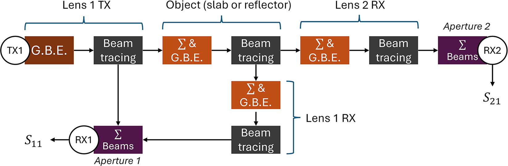
The previously described and implemented tool is used for modeling the setup depicted in Fig. 4, where GBE stands for Gaussian beam expansion. As a beam propagates, it diverges and covers a larger area when intersecting a surface. When the setup elements are not highly coupled, accuracy is maintained by performing a beam summation and field re-expansion right before the element to be modeled. In this simulation setup, four expansion surfaces are established. Ports 1 and 2 are rectangular apertures at which a modal analysis is performed to retrieve the reflection and transmission parameters S 11 and S 21, respectively. The radiation from port 1 is modeled as a Gaussian beam with a 2.11-mm waist. Lenses 1 and 2 are placed at their front focal lengths from their respective ports (i.e., horn aperture). The lenses and the slab are obtained from CAD models imported into the simulator with Gmsh [Reference Geuzaine and Remacle18], allowing the creation of meshes suitable for beam tracing.
Simulation setup. OBJ represents either the sample or the reference mirror.

Figure 5 depicts the pipeline used to model the characterization bench, considering the following assumptions:
• The reflection of the beam on lens 2 does not contribute to the reflection coefficient S 11.
• The reflection of the backward beam on lens 1 does not contribute to the transmission coefficient S 21.
• The lenses are lossless (zero extinction coefficient). Since this loss is present in both calibration and measurement, it is assumed to have no significant impact.
• The power received by the fundamental mode at the aperture is fully transferred into the waveguide.
• Both lenses are perfectly identical in terms of shape and relative permittivity.
Simulation pipeline, where Σ stands for beam summation and G.B.E. for Gaussian beam expansion.

Slab analytical model
An infinite dielectric slab made of rexolite with parallel faces can be modeled using transmission line theory. Given ϵr as the permittivity of the slab, the reflection coefficient of a single interface air-rexolite is
 \begin{equation}
\Gamma = \dfrac{1 - \sqrt{\epsilon_r}}{1 + \sqrt{\epsilon_r}},
\end{equation}
and with γ as the propagation constant in the rexolite, the reflection and transmission coefficients of the dielectric slab under normal incidence can be determined as follows:
 \begin{equation}
S_{11, th} = \dfrac{\Gamma \left( 1 - 2\exp\left\{-2j \gamma h\right\} \right)}{1 - \rho^2 \exp\left\{-2j \gamma h\right\}},
\end{equation}
 \begin{equation}
S_{21, th} = \dfrac{\left( 1 - \Gamma^2 \right) \exp\left\{-2j \gamma h\right\}}{1 - \rho^2 \exp\left\{-2j \gamma h\right\}}.
\end{equation}
For a slab made of an isotropic material, reciprocity is applied, meaning  $S_{22, th} = S_{11, th}$ and
 $S_{12, th} = S_{21, th}$.
Thru-Reflect-Line calibration
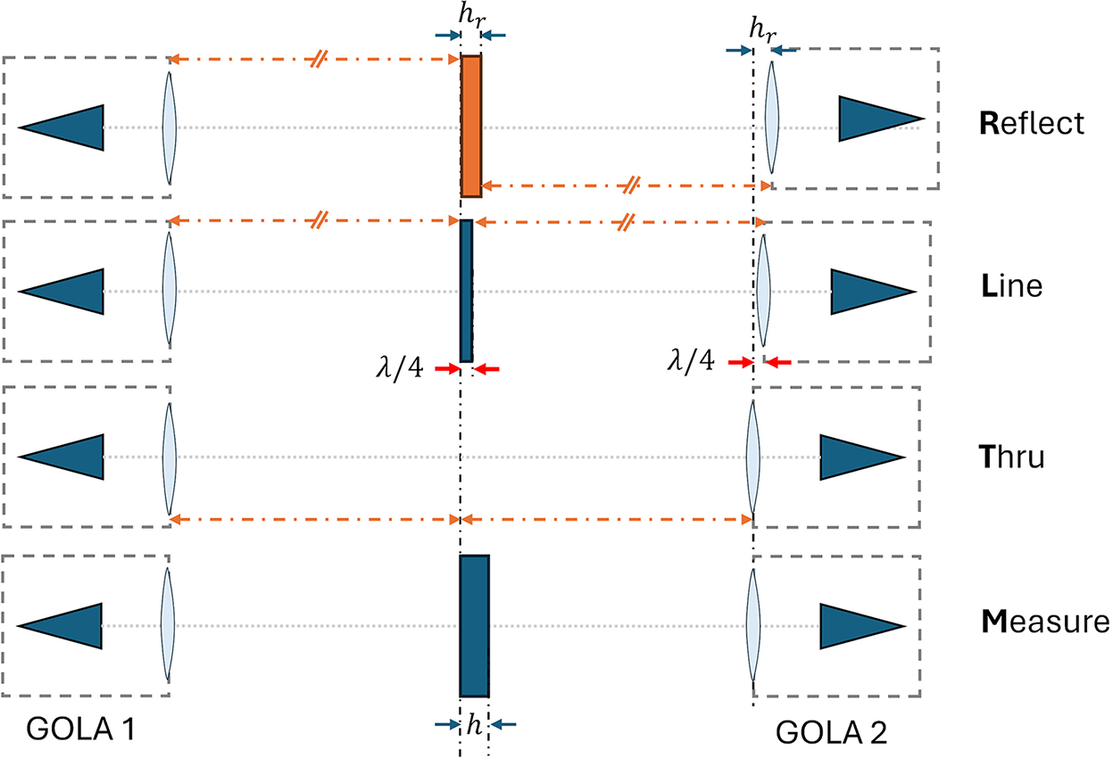
A free-space TRL calibration is carried out on the characterization bench for de-embedding the S-parameters measured with the VNA and thus extract the ones of the slab, a crucial step for accurately extracting its permittivity [Reference Bourreau, Peden and Maguer6]. The procedure involves three steps (denoted as T, R, and L) and is performed only for the direction Port 1  $\rightarrow$ Port 2, under the assumption of perfect symmetry in the simulated system. Therefore, it is assumed that all optical elements are perfectly aligned, representing the ideal case for the bench. We propose here to perform this calibration on the simulated data obtained from the whole setup and compare the results with the dielectric slab theoretical model. In the present study, the element “OBJ” shown in Fig. 4 is substituted by a perfect reflector for step R, an air line of about
 $\frac{\lambda}{4}$ (where λ is the mid-band wavelength) for step L, and then no object for step T. This process is synthesized in Fig. 6.
Principle of the Thru-Reflect-Line calibration applied to the characterization bench for de-embedding the S-parameters.

During a slab measurement, the GOLA at port 2 is not moved and remains in the configuration used for the Thru step. Therefore, in order to compare the simulation to the analytical model of the slab,  $S_{22, th}$,
 $S_{12, th}$ and
 $S_{21, th}$ must be adjusted to the correct reference plane (i.e., the face toward the port 1 of the slab here), giving
 \begin{equation}
S_{22, th, c} = S_{22, th} \cdot \exp\left\{2j k_0 h\right\},
\end{equation}
 \begin{equation}
S_{21, th, c} = S_{21, th} \cdot \exp\left\{j k_0 h\right\}.
\end{equation}
To eliminate any offset caused by misplacement of either the slab or one of the two GOLAs with respect to the reference plane of the TRL, the phase of the product between S 11 and S 22 is utilized to compare with the model.
For each step, results are stored in S2P-format files to be processed by a MATLAB code enabling a TRL calibration.
Results
Simulation of the bench
The simulation involved a frequency sweep from 220 GHz to 330 GHz (over 10 points per GHz) for the three steps (T, R, and L depicted in Fig. 7), followed by the simulation with the slab (defined as step M). The results for the M step are presented in Fig. 8, which shows the simulated S-parameters obtained with and without considering internal reflections within the lenses, as well as the corrected analytical slab S-parameters. Resonances are accurately identified, and the S-parameter magnitudes from both sets exhibit similar trends. The ripples observed in Fig. 8(a) are attributable to multi-reflection inside the lenses, as evidenced by the smoothness of curve in Fig. 8(b), which represents the simulation conducted without internal reflections in the lenses.
Magnitude of simulated S 11 (red) and S 21 (blue) of the bench at 220–330 GHz for the Thru-Reflect-Line steps of the calibration: (a) Thru, (b) Reflect and (c) Line.

Magnitude of raw simulated S-parameters of the bench and analytical S-parameters of the slab at 220–330 GHz with a 12.815-mm rexolite slab ( $\epsilon_r = 2.5329 - 0.00667j$). It is assumed that
 $S_{22} = S_{11}$ and
 $S_{12} = S_{21}$: (a) Simulation with multi-reflections inside lenses and (b) Simulation without multi-reflections inside lenses.

For the frequency sweep involving the four steps (T, R, L, and M), the process typically lasts about 8 hours on a 12-core Intel Core i7-12700H CPU and requires less than 10 GB of RAM. A frequency sweep involving only the step M spans less than 2 hours.
Application of the TRL
A TRL calibration is applied to the simulated S-parameters and presented in Fig. 9. The figure demonstrates a strong agreement between the extracted S-parameters ( $S_{22,s}\cdot S_{11,s}$ and
 $S_{21,s}$), and the corrected analytical S-parameters (
 $S_{22,th,c}\cdot S_{11,th,c}$ and
 $S_{21,th,c}$). Additionally, there is a strong correlation with the measurements of
 $S_{11,m}$ and
 $S_{21,m}$ obtained from the characterization bench. This suggests that using a large beam or a plane wave yields nearly equivalent results under normal incidence.
De-embedded reflection and transmission parameters of the dielectric slab obtained from the simulation, compared to the analytical model and to the measurements, with  $\epsilon_r=2.5329 - 0.00667j$: (a) Module of the transmission parameter, (b) Module of the reflexion parameter, (c) Phase of the transmission parameter and (d) Phase of the transmission parameter.

Next, we study the impact of a misplacement in the characterization bench. Figure 10 shows simulations and measurements with a 15-mm lens horizontal offset from the horn apertures, causing a slightly more focused beam. Although the slab is positioned away from the beam waist, simulations and measurements still well agree, and extracted permittivity remained accurate.
De-embedded reflection and transmission parameters of the slab ( $\epsilon_r=2.5329-0.00667j$). GOLA lenses were shifted horizontally by 15 mm, the slab positioned 150 mm away from the beam waist, and the distance between ports 1 and 2 increased to 1 m: (a) Module of the transmission parameter and (b) Phase of the transmission parameter.

Conclusion
A numerical tool has been implemented to simulate QO systems, such as a free-space characterization bench, at millimeter and sub-millimeter wavelengths. This tool has been employed to simulate a GOLA, a key component of the bench, showing good agreement with measurements obtained using a robotic test bench.
Additionally, it has been demonstrated that this tool can effectively model the entire characterization bench and perform the slab S-parameter de-embedding necessary for permittivity extraction. Future works involve simulating a more realistic bench, accounting for setup imperfections like tilts and misalignments to assess their impact on permittivity extraction accuracy.
Competing interests
The author(s) declare none.

G. Gaudin received his M.Sc. in Engineering from IMT Atlantique, Brest, France, in 2021. During his apprenticeship at Thales Alenia Space, he modeled visible and thermal cameras for vision-based navigation algorithms. He is now a PhD student in Microwave and Quasi-Optical Engineering, focusing on the modeling and design of quasi-optical components for material characterization and non-destructive testing applications.

C. Henry received the M.Sc.Eng. degree from IMT Atlantique, Brest, France, in 2017, the M.Sc. degree from the Chalmers University of Technology, Gothenburg, Sweden, in 2017, and the Ph.D. degree from the Politecnico di Torino, Turin, Italy, in 2021. From December 2021 to October 2022, he was a Post-Doctoral Researcher at IMT Atlantique. Since November 2022, he has been an Associate Professor with the Microwave Department, IMT Atlantique. His research interests include integral equation methods in computational electromagnetics, modeling of complex electromagnetic media, and terahertz imaging.

D. Bourreau obtained his Ph.D. in electronics from the University of Lille, France, in 1989, with much of his work conducted at the University of Limoges. He joined the Lab-STICC laboratory (UMR CNRS 6285) at “Institut Mines Telecom Atlantique,” Brest, France, in 1989. Currently a senior lecturer, his research focuses on microwave power generation up to millimeter-wave (oscillators, frequency multipliers, amplifiers) using combination and quasi-optical techniques, including material characterization.

A. Peden is a Professor at IMT Atlantique, Brest (France). He received his Ph.D. degree in Microwave Electronics from the University of Bretagne Occidentale, Brest, in 1991. Before joining IMT Atlantique (formerly Telecom Bretagne), he worked as an MMIC designer at Thomson Hybrides et Microondes, Orsay, France. His research activities at IMT Atlantique mainly focus on millimeter and sub-millimeter wave applications including quasi-optical techniques for material characterization as well as target characterization and modeling for automotive radar applications.