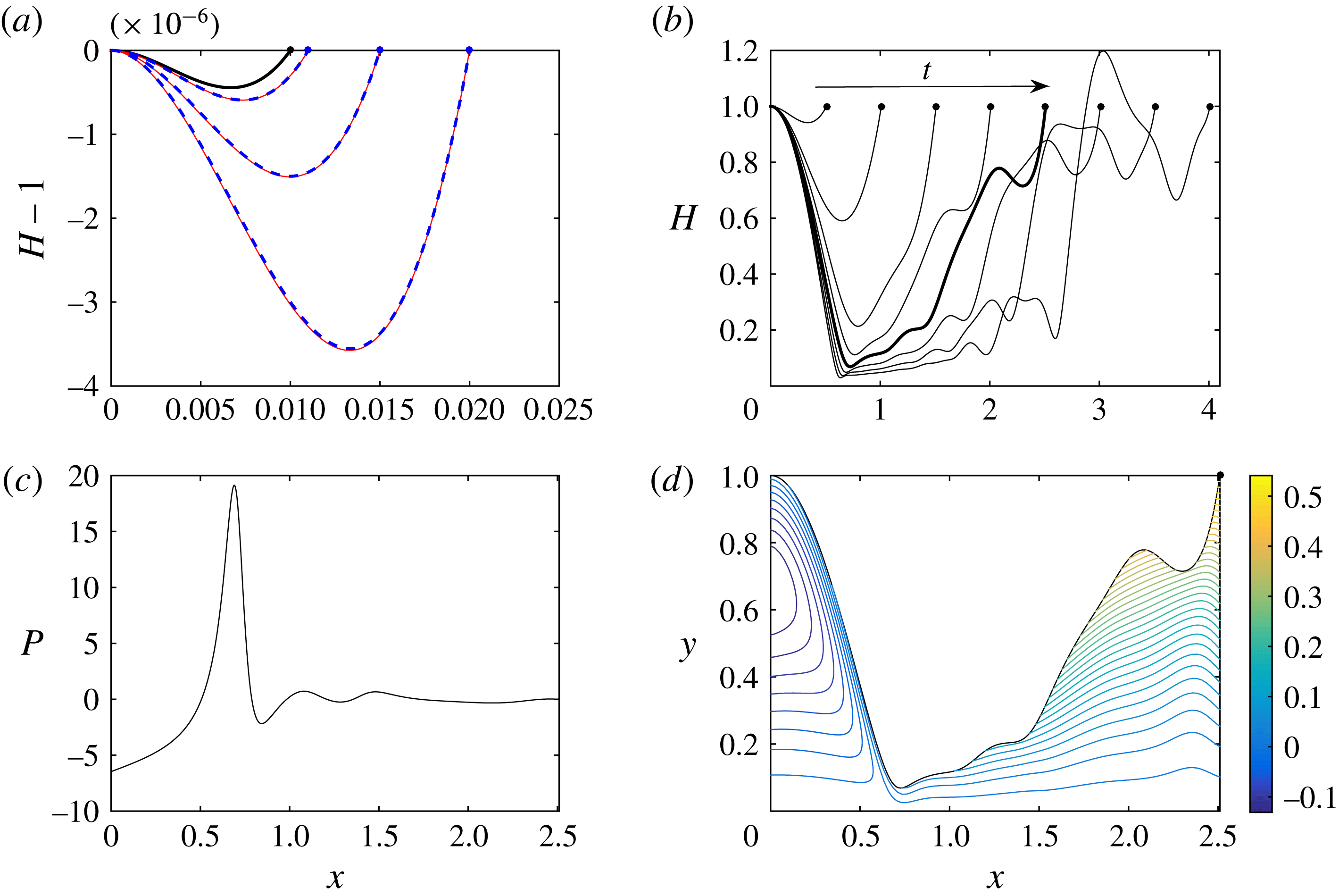
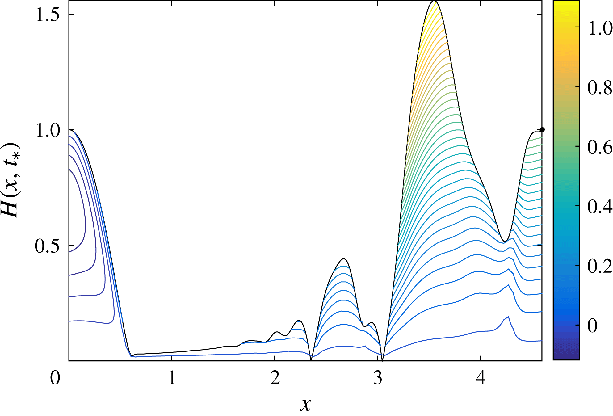
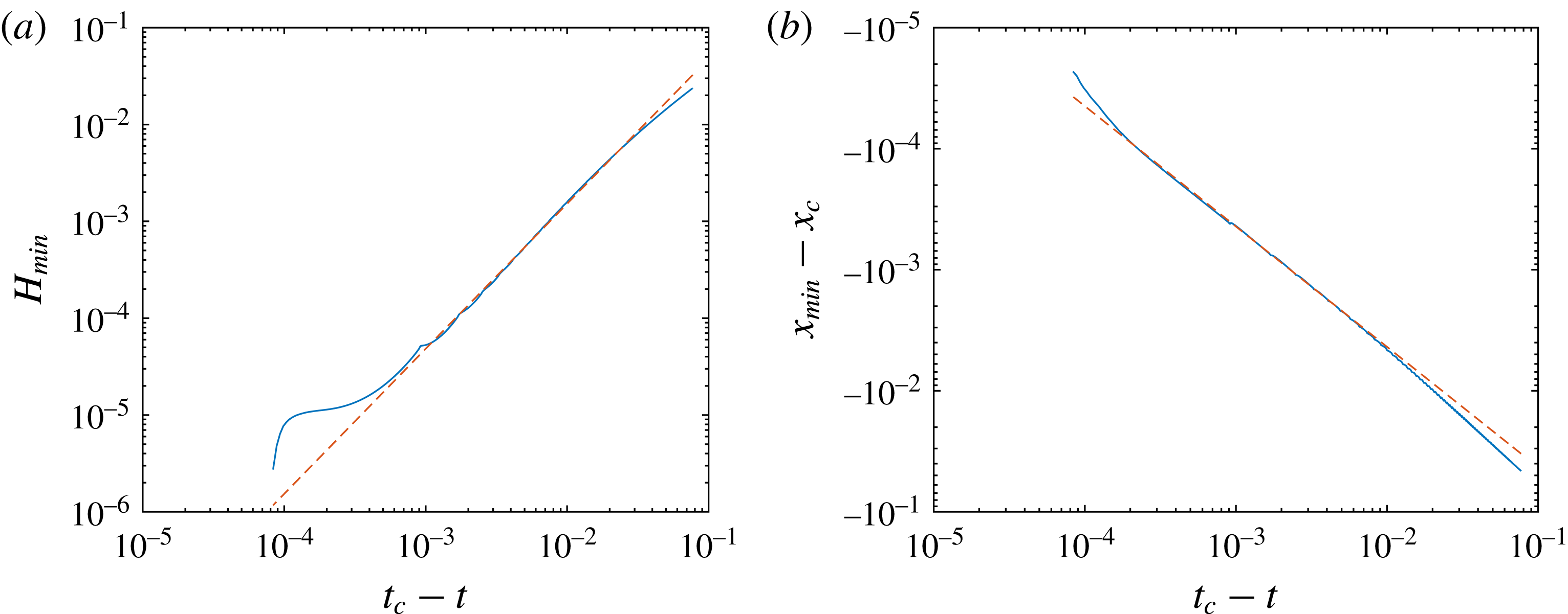
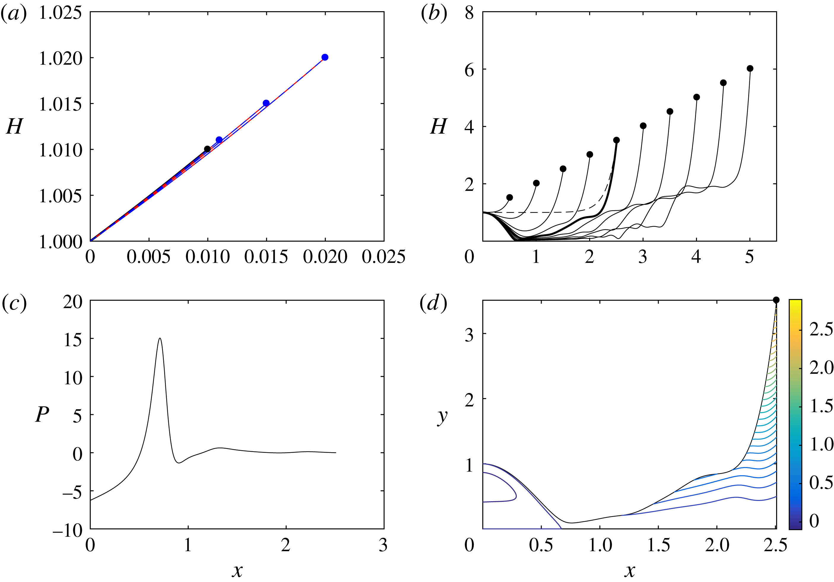
1 Introduction
Liquid jets and sheets are ubiquitous in both industrial processes and natural phenomena. Eggers & Villermaux (Reference Eggers and Villermaux2008) provide a comprehensive review of various applications, ranging from sprays used in agriculture or combustion to the stable liquid sheets necessary for curtain-coating processes or paper production. The promotion of jet or sheet breakup may be beneficial in certain applications (including, e.g., combustion), while its prevention may be essential in others (including, e.g., curtain coating). Thus, an understanding of how liquid jets or sheets interact with the surrounding environment is crucial.
We briefly discuss what we mean by a liquid jet or sheet in this paper. Our particular interest in liquid jets and sheets comes via impact problems and the theory of splashing. When a three-dimensional droplet hits a pool of the same liquid at sufficiently high speed, a thin ‘ejecta’ or splash sheet may be emitted from the neck between the droplet and the pool. In classical two-dimensional impact theory, the analogue of the ejecta is termed the ‘splash jet’; see Howison, Ockendon & Wilson (Reference Howison, Ockendon and Wilson1991). Since the analysis in this paper is purely two-dimensional, we shall use the term ‘jet’ to describe the thin liquid films we study, to be consistent with impact theory, except when referring to experimental papers, where ‘ejecta’ is more appropriate.
Classical impact theory was motivated through applications to ship hydrodynamics, where the vital question is to calculate the force felt by a solid body as it slams into a large volume of liquid; see, for example, Wagner (Reference Wagner1932), Korobkin (Reference Korobkin1985), Armand & Cointe (Reference Armand and Cointe1987), Howison et al. (Reference Howison, Ockendon and Wilson1991) and Oliver (Reference Oliver2007). However, more recently, there has been a growing interest in the application and development of impact theory for the smaller-scale problem of droplet impact, which has practical applications in inkjet printing or spray coating; see Josserand & Thoroddsen (Reference Josserand and Thoroddsen2016) for a review of the recent literature on droplet impact. In these problems, it is of more interest to understand how the droplet splashes and how much liquid is ejected in the splash. Motivated by this need, there has been much recent activity, largely by experimentalists, including, for example, Thoroddsen (Reference Thoroddsen2002), Thoroddsen et al. (Reference Thoroddsen, Thoraval, Takehara and Etoh2011), Thoraval et al. (Reference Thoraval, Takehara, Etoh, Popinet, Ray, Josserand, Zaleski and Thoroddsen2012), Zhang et al. (Reference Zhang, Toole, Fezzaa and Deegan2012a ,Reference Zhang, Toole, Fezzaa and Deegan b ), Thoraval et al. (Reference Thoraval, Takehara, Etoh and Thoroddsen2013), Agbaglah et al. (Reference Agbaglah, Thoraval, Thoroddsen, Zhang, Fezzaa and Deegan2015) and Latka (Reference Latka2017), who consider droplet impacts onto solid substrates or liquid pools, and investigate the formation and dynamics of the ejecta.
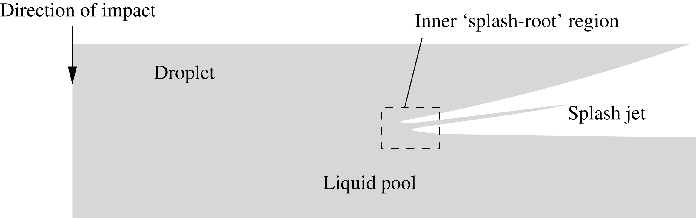
The classical two-dimensional Wagner structure for a droplet impacting a liquid pool at small times when the penetration depth is much smaller than the radius of curvature of the droplet.

Classical inviscid incompressible impact theory – often called Wagner theory after the seminal work of Wagner (Reference Wagner1932) – considers the early stages of impact between a solid and a liquid or between two liquids in the absence of surface tension, gravity and air-cushioning effects. The splash jet forms as a result of the violent displacement of the fluid interface during the impact, as depicted for liquid–liquid impact in figure 1. At small times, when the penetration depth is much smaller than the radius of curvature of the droplet, the jets are governed by the zero-gravity shallow-water equations, with boundary data obtained by matching with the inner ‘splash-root’ regions, as described by, for example, Howison et al. (Reference Howison, Ockendon and Wilson1991). A key assumption in the asymptotic structure is that the jets do not intersect or impact with either the droplet or the pool. However, since the splash jets contribute only a small amount to the hydrodynamic force on the impactor (see, for example, Oliver Reference Oliver2007), their behaviour is mostly neglected in the classical theory.
Our aim in this paper is to give more consideration to the evolution and dynamics of splash jets to help to explain some of the phenomena seen in recent droplet impact experiments. In particular, we explore the role played by surface tension and the surrounding gas, both of which are neglected in Wagner theory. We now describe two specific droplet impact configurations that motivate our analysis, which we outline thereafter.
First, we are motivated by high-Reynolds-number droplet impact onto a liquid pool, as considered by, among others, Thoroddsen et al. (Reference Thoroddsen, Thoraval, Takehara and Etoh2011), Thoraval et al. (Reference Thoraval, Takehara, Etoh, Popinet, Ray, Josserand, Zaleski and Thoroddsen2012), Zhang et al. (Reference Zhang, Toole, Fezzaa and Deegan2012a
,Reference Zhang, Toole, Fezzaa and Deegan
b
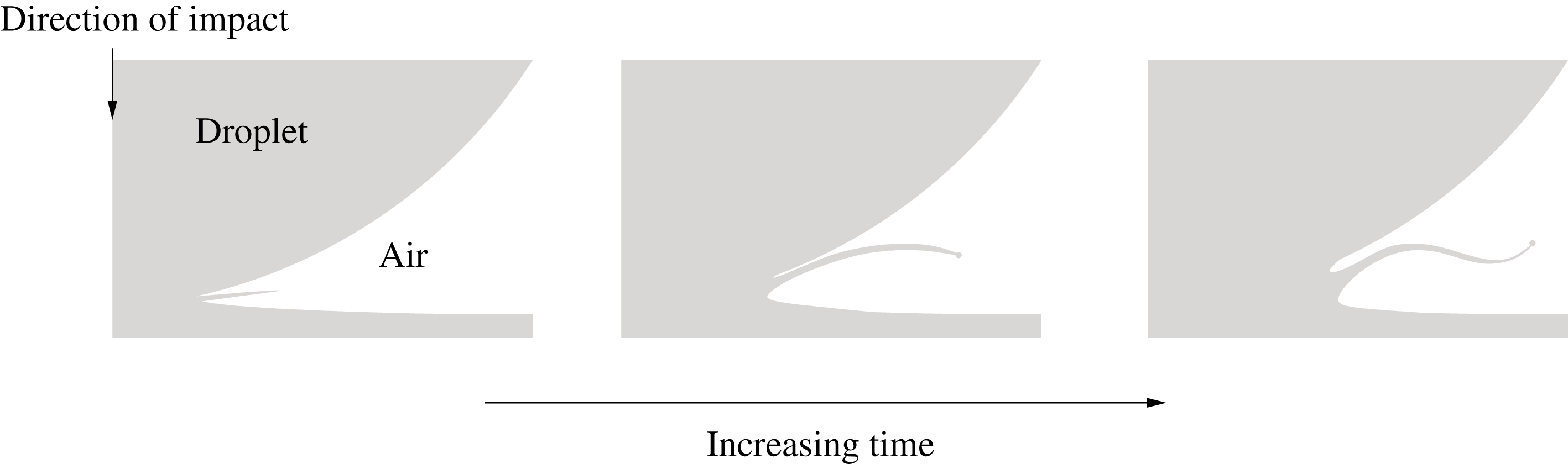
), Thoraval et al. (Reference Thoraval, Takehara, Etoh and Thoroddsen2013) and Agbaglah et al. (Reference Agbaglah, Thoraval, Thoroddsen, Zhang, Fezzaa and Deegan2015). We give in figure 2 a schematic depicting the evolution of the ejecta based on their experiments and simulations. At early stages, the ejecta is emitted at a shallow angle to the undisturbed pool, which is consistent with the Wagner picture. However, at slightly later times, the jet appears to bend, despite being well inside the Wagner regime (the ratio of the penetration depth to the radius of the droplet is approximately
 $10^{-2}$
for the
 $80~\unicode[STIX]{x03BC}\text{s}$
image in figure 2 in Thoraval et al. (Reference Thoraval, Takehara, Etoh, Popinet, Ray, Josserand, Zaleski and Thoroddsen2012), which corresponds to the second schematic in figure 2). Thoroddsen et al. (Reference Thoroddsen, Thoraval, Takehara and Etoh2011) note that eventually the bending ejecta touches down on either the pool or the droplet, causing liquid ligaments to ‘sling-shot’ away from the ejecta. Since it is desirable to reduce the amount of liquid lost to satellite droplets in, for example, inkjet printing, an understanding of why ejectas can behave in this violent manner is clearly an issue of fundamental importance. Cylinders of air are also trapped in the drop as the ejecta touches down. These cylinders then break up due to Rayleigh instability, forming rings of air bubbles; see, for example, Thoraval et al.
Reference Thoraval, Takehara, Etoh and Thoroddsen2013. Air bubbles can lead to imperfections in, for example, coating applications.
Bending of an ejecta during droplet impact onto a liquid pool: a schematic based on a cross-sectional view of experiments by Thoroddsen et al. (Reference Thoroddsen, Thoraval, Takehara and Etoh2011) and simulations by Thoraval et al. (Reference Thoraval, Takehara, Etoh, Popinet, Ray, Josserand, Zaleski and Thoroddsen2012).

There are elements missing from the Wagner model that may explain these dynamics, and, in particular, Thoroddsen et al. (Reference Thoroddsen, Thoraval, Takehara and Etoh2011) suggest that the surrounding air is responsible for the deflection of the ejecta. They propose a ballistic model for the ejecta evolution incorporating a term representing air drag on its rim. Numerical simulations of their model give qualitatively similar pictures to the experiments. However, they do not consider the role of the air between the ejecta and the two liquid domains. At early stages, these air layers are thin, which suggests that lubrication pressures may build up, which, in turn, could also cause the ejecta to bend.
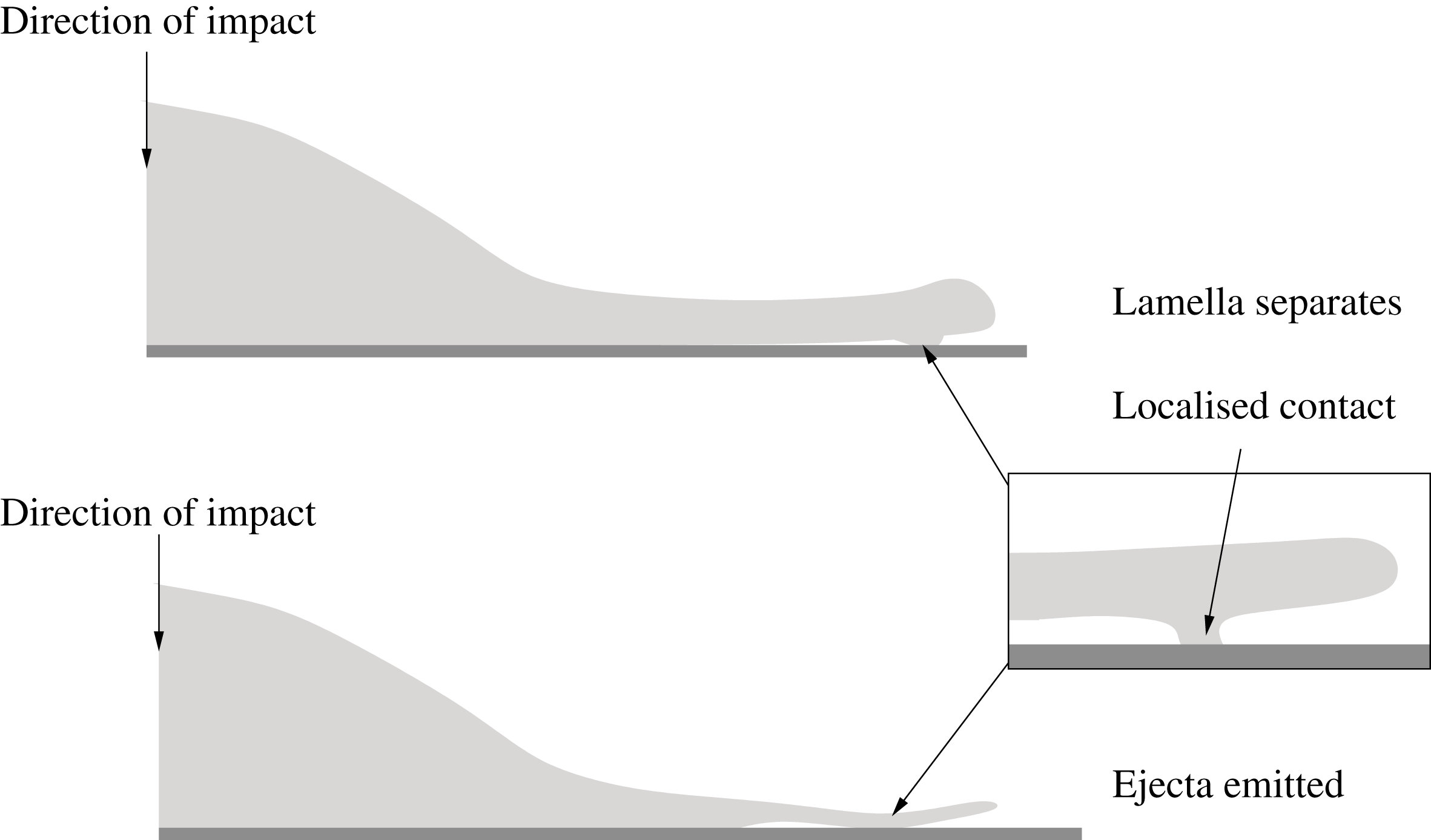
A cross-sectional view of separation and localised touchdown of a spreading droplet front. The top image shows the touchdown of a lamella that has become separated from a substrate, based on Thoroddsen, Takehara & Etoh (Reference Thoroddsen, Takehara and Etoh2010), while the bottom image shows localised touchdown of an ejecta emitted from the front of a lamella, based on Driscoll, Stevens & Nagel (Reference Driscoll, Stevens and Nagel2010).

The second motivation comes from higher-viscosity – although still high-Reynolds-number – impacts. In such impacts, a droplet impinging on a solid substrate may spread as opposed to splash, as illustrated schematically in figure 3. However, experiments by, among others, Driscoll et al. (Reference Driscoll, Stevens and Nagel2010), Thoroddsen et al. (Reference Thoroddsen, Takehara and Etoh2010) and Palacios et al. (Reference Palacios, Hernández, Gómez, Zanzi and López2012) have shown that the advancing droplet front – also called the lamella – may entrain bubbles of air. Schroll et al. (Reference Schroll, Josserand, Zaleski and Zhang2010) show that the lamella may become detached from the substrate as the droplet spreads, so that a cushioning layer of air is trapped between the lamella and the solid. They link this separation to the detachment of the boundary layer within the spreading droplet. Thoroddsen et al. (Reference Thoroddsen, Takehara and Etoh2010) use this separation to suggest a possible mechanism for the entrainment of air bubbles: as the lamella advances, it touches down ahead of the advancing contact line, causing the entrapment of a volume of air. This mechanism is depicted in figure 3. However, Driscoll et al. (Reference Driscoll, Stevens and Nagel2010) give a slightly different mechanism, connected to the emission of an ejecta from the front of the lamella. Driscoll et al. (Reference Driscoll, Stevens and Nagel2010) directly link ejecta formation to air entrainment, showing that if the air pressure is reduced significantly, the ejecta is suppressed and no bubbles of air are entrapped. This conclusion is supported by experiments by Driscoll & Nagel (Reference Driscoll and Nagel2011) and de Ruiter et al. (Reference de Ruiter, Oh, van den Ende and Mugele2012). Nevertheless, when the ejecta does form, it rides on a thin air cushion, leading to entrapment, as depicted in the inset to figure 3.
The influence of the surrounding air on the jet produced as a flat plate enters water was investigated by Yakimov (Reference Yakimov1973) and has often been cited as the source of discrepancies between Wagner theory and experiments; see, for example, Howison et al. (Reference Howison, Ockendon and Wilson1991) and references therein. In particular, Xu, Zhang & Nagel (Reference Xu, Zhang and Nagel2005) showed that splashing can be completely inhibited in droplet impact on a solid surface by lowering the ambient air pressure: at a critical value of the gas pressure, the droplet spreads rather than splashes. This idea was expanded by, among others, Driscoll et al. (Reference Driscoll, Stevens and Nagel2010) and Latka et al. (Reference Latka, Strandburg-Peshkin, Driscoll, Stevens and Nagel2012). Numerous authors have considered the role of the ambient gas in impact theory, both before impact, for example Wilson (Reference Wilson1991) and Smith, Li & Wu (Reference Smith, Li and Wu2003), and after impact, for example Purvis & Smith (Reference Purvis and Smith2004), Hicks & Purvis (Reference Hicks and Purvis2010), Duchemin & Josserand (Reference Duchemin and Josserand2011), Moore, Ockendon & Oliver (Reference Moore, Ockendon and Oliver2013), Moore & Oliver (Reference Moore and Oliver2014), Josserand, Ray & Zaleski (Reference Josserand, Ray and Zaleski2016) and Jian et al. (Reference Jian, Josserand, Popinet, Ray and Zaleski2018). We also note that air entrainment has been linked by Rein & Delplanque (Reference Rein and Delplanque2008) to so-called ‘corona splashes’, where the lamella of a spreading droplet is lifted at a much larger angle away from the substrate, forming a liquid crown that can break up into droplets. Liquid crowns are considered in detail by, for example, Yarin & Weiss (Reference Yarin and Weiss1995), Roisman & Tropea (Reference Roisman and Tropea2002) and Edwards et al. (Reference Edwards, Howison, Ockendon and Ockendon2008).
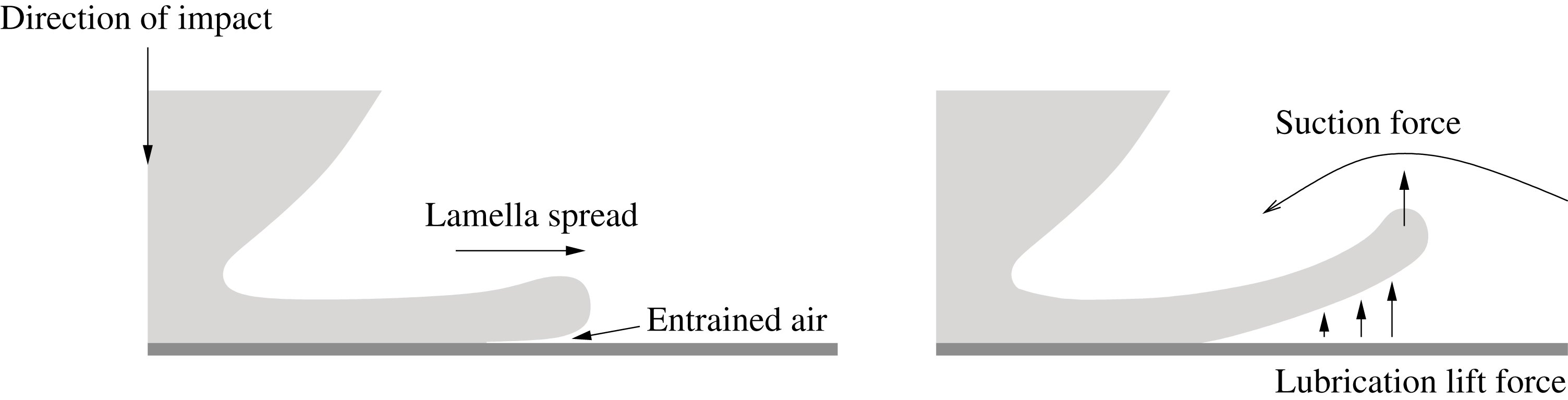
In a series of recent studies, Riboux & Gordillo (Reference Riboux and Gordillo2014, Reference Riboux and Gordillo2015, Reference Riboux and Gordillo2017) have considered the role of the surrounding air in the earliest stages of lamella growth and detachment in droplet impact onto solid substrates. Riboux & Gordillo (Reference Riboux and Gordillo2014) utilise the theory of Marchand et al. (Reference Marchand, Chan, Snoeijer and Andreotti2012) to show that the relevant droplet capillary numbers are well above the critical value at which the expanding lamella begins to dewet from its tip, as depicted in the schematic in figure 4. After dewetting, Riboux & Gordillo (Reference Riboux and Gordillo2014) then derive a criterion for splashing, whereby the detached lamella lifts away from the substrate faster than the lamella rim grows due to Taylor–Culick retraction. The forces acting on the lamella are estimated by considering two separate problems: first, a lift force due to the thin lubricating air layer under the dewetted lamella and, second, a suction force due to the flow over the lamella rim (see figure 4 for an illustration). In the limit in which the lubrication force dominates, they show good comparisons with their own experiments and those by Palacios et al. (Reference Palacios, Hernández, Gómez, Zanzi and López2012).
A schematic depicting the detachment and ‘splash’ of an advancing lamella, as studied by Riboux & Gordillo (Reference Riboux and Gordillo2014). For sufficiently large capillary number, the expanding rim of the lamella entrains an air layer. The lubrication forces in this thin layer along with the suction caused by the air flowing over the tip lead to the lamella deflecting away from the substrate, provided that the vertical speed of the lamella rim exceeds the growth rate of the rim under the action of surface tension.

Riboux & Gordillo (Reference Riboux and Gordillo2015) extend the analysis by considering the motion of a lamella once it has detached from the substrate. By considering the deceleration of the lamella as it spreads, Riboux & Gordillo (Reference Riboux and Gordillo2015) derive the viscous correction term to the predictions of Wagner theory for the location of the lamella root and its thickness there. The predictions are then supplied as boundary conditions to a ballistic model for the lamella, where the zero-gravity shallow-water equations of Wagner theory – see Howison et al. (Reference Howison, Ockendon and Wilson1991) – are solved for the lamella thickness and tangential velocity. These simulations are then coupled with an approximate model for the growth of the lamella rim, which is assumed to be cylindrical due to the local effects of surface tension. The effect of the boundary layer in the Wagner jet-root region is considered in Riboux & Gordillo (Reference Riboux and Gordillo2017), leading to a refined approximation for the splashing condition derived in Riboux & Gordillo (Reference Riboux and Gordillo2014).
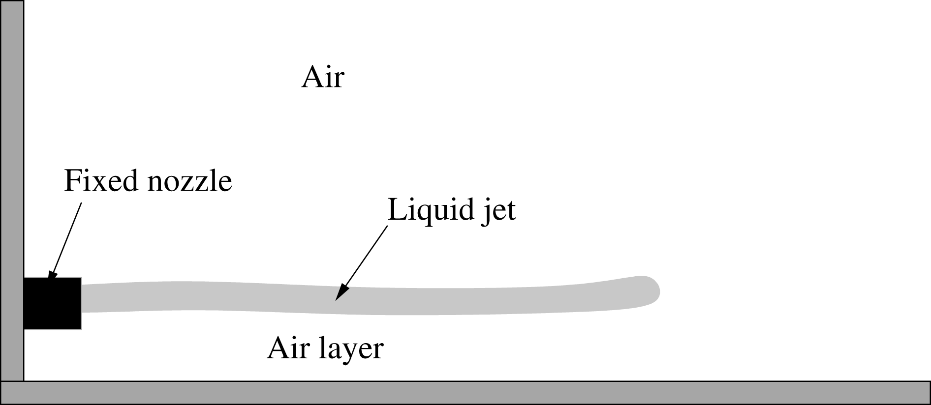
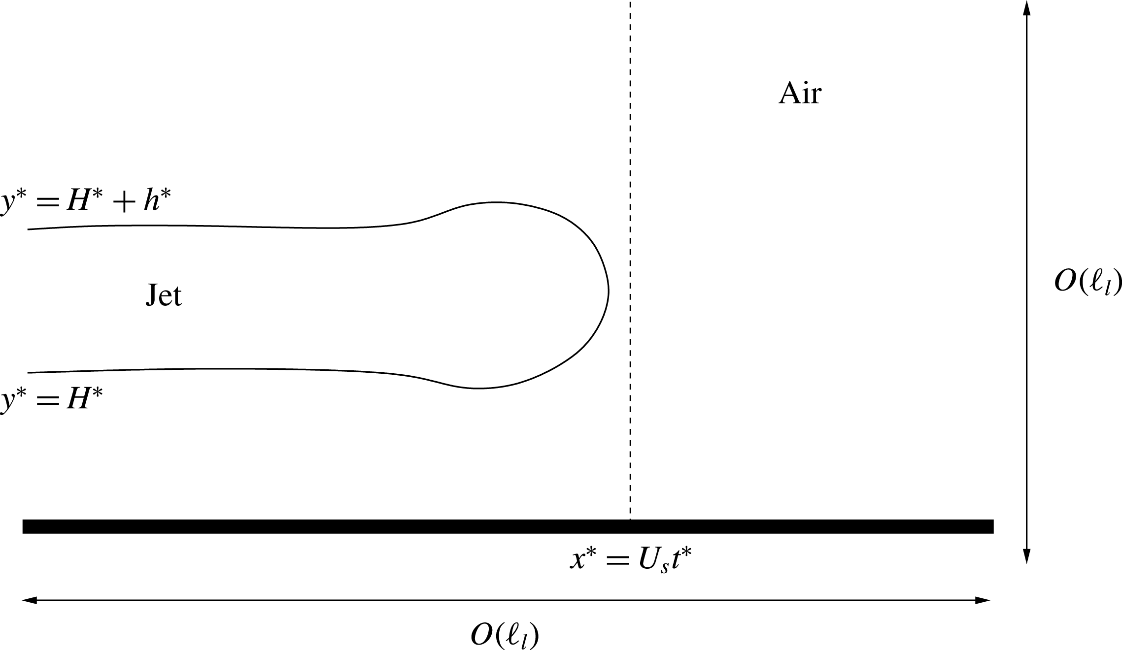
In this paper, we will consider a simplified canonical model in which a thin liquid jet is shot from a nozzle over a solid substrate into initially quiescent air, as illustrated in figure 5. The nozzle is not necessarily aligned parallel to the substrate, but we assume that the angle it makes to the substrate is small, which is the appropriate limit for early-time ejecta formation. As it grows, the jet traps a thin air-cushioning layer between its lower free boundary and the solid substrate. This simplification allows us to investigate the conditions under which the jet may bend due to the large air pressures in the cushioning layer, giving us a possible mechanism for lamella touchdown in the more complicated impact scenarios illustrated in figures 2–4. In particular, by considering our idealised configuration, we aim to build upon the models discussed above. We emphasise that we shall concentrate on the evolution of a thin jet in the presence of an air-cushioning layer given that the jet has formed. Our primary aim is to perform a systematic derivation of the governing equations for the evolution of a thin jet in the presence of a thin air-cushioning layer. This differs from the analysis of Riboux & Gordillo (Reference Riboux and Gordillo2014, Reference Riboux and Gordillo2015) both in that each of the fluid layers is taken to be thin – the thickness of the lamella is neglected in the lubrication approximations of the entrained air layer in Riboux & Gordillo (Reference Riboux and Gordillo2014) – while we also include a model for the evolution of the centreline of the splash jet, which is not considered in Riboux & Gordillo (Reference Riboux and Gordillo2015). Moreover, when we move on to consider the growth of a jet of finite length, our analysis of the tip region also incorporates the presence of the solid substrate, which is not considered in Riboux & Gordillo (Reference Riboux and Gordillo2015), but which will undoubtedly play a role in the early stages of lamella detachment. Finally, since we arrive at our model following a systematic reduction of the full Navier–Stokes equations, we establish the regimes in which the zero-gravity shallow-water approximation in the jet seen in Wagner theory is reasonable.
A simplified model to investigate the influence of a thin air cushion on a liquid jet. The jet shoots from a nozzle attached to a solid wall into a region of initially quiescent air. The nozzle is aligned almost parallel to a solid substrate, but a fixed height above the substrate.

We emphasise that, in this paper, we do not consider the mechanism by which a thin splash jet may be formed (other than within the context of Wagner theory as described above). Rather, we look at its evolution in the presence of an air-cushioning layer given that a thin jet has formed. The question of how the splash originates is an important question in its own right, with several authors arguing theoretically (e.g. Mandre, Mani & Brenner Reference Mandre, Mani and Brenner2009; Mani, Mandre & Brenner Reference Mani, Mandre and Brenner2010; Mandre & Brenner Reference Mandre and Brenner2012) and experimentally (e.g. Kolinski et al. Reference Kolinski, Rubinstein, Mandre, Brenner, Weitz and Mahadevan2012; Kolinski, Mahadevan & Rubinstein Reference Kolinski, Mahadevan and Rubinstein2014; Liu, Tan & Xu Reference Liu, Tan and Xu2015) that droplets impacting a solid surface begin to spread over a nanometre-sized air layer before they touch the substrate. Indeed, Liu et al. (Reference Liu, Tan and Xu2015) use specially designed porous substrates to show that draining the air under an impacting drop prevents splashing from occurring at all. The air layers involved in the origin of the splash jet are incredibly thin – indeed, the continuum assumption is called into question (see, for example, Sprittles Reference Sprittles2017) – and we do not consider them here.
It is also important to emphasise that our interest is not in jet breakup and disintegration into satellite droplets, but rather in the stability and deflection of the centreline: in figure 2, the jet undulates on a faster time scale than it disintegrates. In general, most of the work on jet evolution and instability, inspired by the work of Rayleigh (1878) on cylindrical jets and Taylor (Reference Taylor1959) on liquid sheets, concentrates on jet breakup and the size of the resulting droplets that form. Moreover, in general, the dynamics of the surrounding air is neglected, although there are several notable exceptions, as we shall now briefly discuss to put into sharper contrast the models that we shall develop in this paper.
Weber (Reference Weber1931) extends the work of Rayleigh (1878) and suggests that air–liquid interactions at the jet interface can enhance disturbances to the jet motion. In particular, a large velocity difference between the gas and the jet increases the instability of the jet to small sinusoidal perturbations. Squire (Reference Squire1953) considers the stability of a two-dimensional sheet in an ambient medium, although the air is stationary in its base state. Dombrowski & Hooper (Reference Dombrowski and Hooper1962) compare the stability analyses of Squire (Reference Squire1953) and Hagerty & Shea (Reference Hagerty and Shea1955) with experiments in which a laminar sheet is formed from a single nozzle. They show that as the ambient air density is reduced, breakup of the sheet can be inhibited. Sterling & Sleicher (Reference Sterling and Sleicher1975), Li & Tankin (Reference Li and Tankin1991) and Li (Reference Li1993) extend the model further by retaining the viscosity of the liquid in the jet.
Teng, Lin & Chen (Reference Teng, Lin and Chen1997) consider a viscous liquid sheet enveloped by two viscous air layers bounded by solid walls. They derive the Orr–Sommerfeld equation governing the stability of the base-state constant-thickness sheet to small perturbations. They derive a critical Weber number below which the flow is absolutely unstable. For larger Weber numbers, the flow is convectively unstable: this instability is caused by the amplification of small disturbances near the gas–liquid interface. Söderberg & Alfredsson (Reference Söderberg and Alfredsson1998) consider a similar problem without the bounding walls: the base-state gas flow is approximated by assuming that the sheet acts as a moving wall and applying Stokes boundary layer theory.
Gordillo, Pérez-Saborid & Gañán-Calvo (Reference Gordillo, Pérez-Saborid and Gañán-Calvo2001) perform an analysis of a thin inviscid liquid jet in a co-flowing gas stream to simulate atomisation of liquid sprays. They adopt various base-state profiles of the liquid and gas velocities, finding that these base flows play an important role in the stability of the jet at sufficiently large Weber numbers.
Tammisola et al. (Reference Tammisola, Sasaki, Lundell, Matsubara and Söderberg2011) investigate the conditions under which the surrounding gas flow stabilises a liquid sheet that is subject to infinitesimal interfacial perturbations. To model the base air flow, they adopt both the Stokes approximation of Söderberg & Alfredsson (Reference Söderberg and Alfredsson1998) as well as an alternative approximation of the air flow using a boundary layer approach. They perform a theoretical, numerical and experimental investigation into sheet stability and show that the size of the predicted disturbance depends strongly on the velocity difference between the air and the liquid, as well as the effect of the air shear on the sheet free surface. In particular, when the base-state liquid and air speeds are very close, instability is inhibited, in agreement with Weber (Reference Weber1931). Tammisola, Lundell & Söderberg (Reference Tammisola, Lundell and Söderberg2012) extend the analysis to investigate the role of surface tension and inlet shear.
Our analysis will differ from these works in two ways. First, our jets will be riding on a very thin air layer, which will play a key role in the stability of a spatially uniform infinite jet (or, equivalently, a local-in-space-and-time analysis of a very long jet) to small sinusoidal perturbations of (effectively) its centreline. Second, as depicted in figure 5, we shall move on to consider the effects of jet growth and, in particular, attempt to incorporate the role of the air in front of the jet near the tip and near its root (i.e. near the nozzle in figure 5).
We note that several of the models we derive share characteristics with those for extensional flows. Among others, Dewynne, Ockendon & Wilmott (Reference Dewynne, Ockendon and Wilmott1992), Dewynne, Howell & Wilmott (Reference Dewynne, Howell and Wilmott1994), Howell (Reference Howell1994), van de Fliert, Howell & Ockendon (Reference van de Fliert, Howell and Ockendon1995), Howell (Reference Howell1996), Filippov & Zheng (Reference Filippov and Zheng2010) and Pfingstag, Audoly & Boudaoud (Reference Pfingstag, Audoly and Boudaoud2011) consider a variety of extensions to the classical gravity-driven extensional flow of Trouton (Reference Trouton1906), with the work of van de Fliert et al. (Reference van de Fliert, Howell and Ockendon1995) of particular relevance here, since it considers the evolution of a viscous thread under an external pressure gradient. We shall highlight important similarities where appropriate.
We now outline the plan for the paper. In § 2, we shall formulate a model in which an infinite liquid jet flows over a solid substrate above a thin air-cushioning layer. In § 3, we discuss the modelling assumptions and derive the length scales over which deflections to the jet are caused by an air pressure jump across it in various asymptotic regimes depending on the size of the relevant reduced Reynolds numbers in the jet and air layer. In § 4, we derive the leading-order model in four specific regimes in which the reduced Reynolds numbers in the air and jet are either large or small. We will discuss the linear stability of the jet in § 5, showing that its centreline can become unstable to small perturbations in the pressure and thickness of the air layer in each of our asymptotic regimes, provided that surface tension is not too strong. We move on to discuss a growing jet with tip effects in § 6, where we derive asymptotic and numerical solutions for the simplest possible model in which a constant-speed, constant-thickness jet is shot parallel to a solid substrate. In § 7, we discuss the applicability of our models to several recent experimental studies. We conclude by summarising our main results and highlighting areas for future work.
2 Formulation of the problem
In order to investigate the influence of a thin air-cushioning layer on a thin liquid jet, we consider a canonical problem in which a two-dimensional liquid jet moves over a planar rigid impermeable substrate with an air layer sandwiched between the jet and the substrate, as we depicted in figure 5. Since the model has the potential to be quite complicated, we shall defer a discussion of the role of the nozzle and the jet tip to § 6 and derive a model for an infinite liquid jet.
We suppose that the jet moves with typical horizontal speed
 $U_{s}$
and has a typical thickness
 $\ell _{l}$
, while the air layer is assumed to have a typical thickness
 $\ell _{g}$
. The liquid density
 $\unicode[STIX]{x1D70C}_{l}$
and viscosity
 $\unicode[STIX]{x1D707}_{l}$
, as well as the air density
 $\unicode[STIX]{x1D70C}_{g}$
and viscosity
 $\unicode[STIX]{x1D707}_{g}$
, are all assumed to be constant, with the liquid/air both being Newtonian. The constant liquid–air surface tension is denoted by
 $\unicode[STIX]{x1D70E}$
. Gravity acts downwards, perpendicular to the solid substrate, and the acceleration due to gravity is denoted by
 $g$
. An important part of our analysis will be to determine the length scale
 $L$
over which the pressure in the cushioning layer causes a transverse deflection to the jet centreline of order
 $\ell _{g}$
. We denote the aspect ratios of the jet and the cushioning layer by
 $\unicode[STIX]{x1D700}_{i}=\ell _{i}/L$
, where
 $i=l,g$
respectively. Throughout this analysis, we shall take
 $\unicode[STIX]{x1D700}_{i}\ll 1$
.
For the rest of our analysis, variables in the jet are denoted by a lower-case letter and variables in the air by an upper-case letter, and we shall use an asterisk to denote a dimensional variable. We introduce Cartesian coordinates
 $(x^{\ast },y^{\ast })$
, so that
 $y^{\ast }=0$
aligns with the solid substrate, and denote time by
 $t^{\ast }$
. The velocities in the jet and air are denoted by
 $\boldsymbol{u}^{\ast }=(u^{\ast }(x^{\ast },y^{\ast },t^{\ast }),v^{\ast }(x^{\ast },y^{\ast },t^{\ast }))^{\text{T}}$
and
 $\boldsymbol{U}^{\ast }=(U^{\ast }(x^{\ast },y^{\ast },t^{\ast }),V^{\ast }(x^{\ast },y^{\ast },t^{\ast }))^{\text{T}}$
respectively. Moreover, the liquid and air pressures are denoted by
 $p^{\ast }(x^{\ast },y^{\ast },t^{\ast })$
and
 $P^{\ast }(x^{\ast },y^{\ast },t^{\ast })$
. We differentiate between the upper and lower free surfaces of the jet by denoting the lower free surface by
 $y^{\ast }=H^{\ast }(x^{\ast },t^{\ast })$
and the upper free surface by
 $y^{\ast }=H^{\ast }(x^{\ast },t^{\ast })+h^{\ast }(x^{\ast },t^{\ast })$
.
A useful simplification is to neglect the initially quiescent upper unbounded air region since we expect the thinness of the cushioning air layer to produce air pressures that are much larger than those generated above. We shall verify this assumption a posteriori. We note that this assumption would be violated if there were a tip: local to the tip, we would expect the air above the jet to play an important role in the dynamics; see appendix C.
Under the assumptions listed above, the flow of liquid and air is governed by the incompressible Navier–Stokes equations subject to the usual no-slip, no-flux boundary conditions on the substrate and the usual kinematic, continuity and dynamic boundary conditions on the free surfaces. In addition, we shall require sufficient inlet and initial conditions to close the problem. We shall discuss suitable conditions for our reduced models in § 6.
For brevity, we will present the governing equations in non-dimensional form only. We non-dimensionalise
 $x^{\ast }$
by
 $L$
;
 $y^{\ast }$
by
 $\unicode[STIX]{x1D700}_{i}L$
, where
 $i=l,g$
in the liquid and air respectively;
 $t^{\ast }$
by
 $L/U_{s}$
;
 $H^{\ast }$
by
 $\unicode[STIX]{x1D700}_{g}L$
;
 $h^{\ast }$
by
 $\unicode[STIX]{x1D700}_{l}L$
;
 $u^{\ast },U^{\ast }$
by
 $U_{s}$
;
 $v^{\ast },V^{\ast }$
by
 $\unicode[STIX]{x1D700}_{l}U_{s}$
and
 $\unicode[STIX]{x1D700}_{g}U_{s}$
respectively; and
 $p^{\ast }$
,
 $P^{\ast }$
by
 $\unicode[STIX]{x1D70C}_{l}U_{s}^{2}$
,
 ${\mathcal{P}}_{g}$
, where the air pressure scale,
 ${\mathcal{P}}_{g}$
, will vary depending on the asymptotic limit we wish to consider. We shall denote the dimensionless vertical coordinate by
 $\bar{y}$
in the jet and by
 ${\hat{y}}$
in the air layer, and the ratio of the jet and air layer aspect ratios by
 $\unicode[STIX]{x1D702}=\unicode[STIX]{x1D700}_{g}/\unicode[STIX]{x1D700}_{l}$
.
Under these scalings, the incompressible Navier–Stokes equations in the jet (
 $\unicode[STIX]{x1D702}H<\bar{y}<\unicode[STIX]{x1D702}H+h$
) are given by
 $$\begin{eqnarray}\displaystyle & \displaystyle \unicode[STIX]{x1D700}_{l}^{2}\,\mathit{Re}_{l}(u_{t}+uu_{x}+vu_{\bar{y}})=-\unicode[STIX]{x1D700}_{l}^{2}\,\mathit{Re}_{l}\,p_{x}+\unicode[STIX]{x1D700}_{l}^{2}u_{xx}+u_{\bar{y}\bar{y}}, & \displaystyle\end{eqnarray}$$
 $$\begin{eqnarray}\displaystyle & \displaystyle \unicode[STIX]{x1D700}_{l}^{2}\,\mathit{Re}_{l}(v_{t}+uv_{x}+vv_{\bar{y}})=-\mathit{Re}_{l}\,p_{\bar{y}}+\unicode[STIX]{x1D700}_{l}^{2}v_{xx}+v_{\bar{y}\bar{y}}-\frac{\unicode[STIX]{x1D700}_{l}\,\mathit{Re}_{l}}{\mathit{Fr}^{2}}, & \displaystyle\end{eqnarray}$$
 $$\begin{eqnarray}\displaystyle & u_{x}+v_{\bar{y}}=0, & \displaystyle\end{eqnarray}$$
and in the air layer below the jet
 $(0<{\hat{y}}<H)$
they are given by
 $$\begin{eqnarray}\displaystyle & \unicode[STIX]{x1D700}_{g}^{2}\,\mathit{Re}_{g}(U_{t}+UU_{x}+VU_{{\hat{y}}})=-{\mathcal{Q}}P_{x}+\unicode[STIX]{x1D700}_{g}^{2}U_{xx}+U_{{\hat{y}}{\hat{y}}}, & \displaystyle\end{eqnarray}$$
 $$\begin{eqnarray}\displaystyle & \displaystyle \unicode[STIX]{x1D700}_{g}^{4}\,\mathit{Re}_{g}(V_{t}+UV_{x}+VV_{{\hat{y}}})=-{\mathcal{Q}}P_{{\hat{y}}}+\unicode[STIX]{x1D700}_{g}^{4}V_{xx}+\unicode[STIX]{x1D700}_{g}^{2}V_{{\hat{y}}{\hat{y}}}-\frac{\unicode[STIX]{x1D700}_{g}^{3}\,\mathit{Re}_{g}}{\mathit{Fr}^{2}}, & \displaystyle\end{eqnarray}$$
 $$\begin{eqnarray}\displaystyle & U_{x}+V_{{\hat{y}}}=0, & \displaystyle\end{eqnarray}$$
where the Froude and Reynolds numbers in the liquid and air are defined by
 $$\begin{eqnarray}\mathit{Fr}=\frac{U_{s}}{\sqrt{gL}},\quad \mathit{Re}_{l}=\frac{\unicode[STIX]{x1D70C}_{l}LU_{s}}{\unicode[STIX]{x1D707}_{l}},\quad \mathit{Re}_{g}=\frac{\unicode[STIX]{x1D70C}_{g}LU_{s}}{\unicode[STIX]{x1D707}_{g}}\end{eqnarray}$$
respectively, and the pressure coefficient is defined as
 $$\begin{eqnarray}{\mathcal{Q}}=\frac{\unicode[STIX]{x1D700}_{g}^{2}{\mathcal{P}}_{g}L}{\unicode[STIX]{x1D707}_{g}U_{s}}.\end{eqnarray}$$
On the solid surface, we require no-slip and no-flux conditions, so that
 $$\begin{eqnarray}U=V=0\quad \text{on}~{\hat{y}}=0.\end{eqnarray}$$
The kinematic boundary conditions on the free surfaces are given by
 $$\begin{eqnarray}\displaystyle & V=H_{t}+uH_{x}\quad \text{on}~{\hat{y}}=H, & \displaystyle\end{eqnarray}$$
 $$\begin{eqnarray}\displaystyle & v=\unicode[STIX]{x1D702}(H_{t}+uH_{x})\quad \text{on}~\bar{y}=\unicode[STIX]{x1D702}H, & \displaystyle\end{eqnarray}$$
 $$\begin{eqnarray}\displaystyle & v=\unicode[STIX]{x1D702}(H_{t}+uH_{x})+h_{t}+uh_{x}\quad \text{on}~\bar{y}=\unicode[STIX]{x1D702}H+h. & \displaystyle\end{eqnarray}$$
The continuity of velocity conditions on the lower free surface are given by
 $$\begin{eqnarray}u(x,\unicode[STIX]{x1D702}H,t)=U(x,H,t),\quad v(x,\unicode[STIX]{x1D702}H,t)=\unicode[STIX]{x1D702}V(x,H,t).\end{eqnarray}$$
Neglecting the air above the jet, the normal stress condition on
 $\bar{y}=\unicode[STIX]{x1D702}H+h$
is given by
 $$\begin{eqnarray}\displaystyle p & = & \displaystyle -\frac{\unicode[STIX]{x1D700}_{l}(\unicode[STIX]{x1D702}H_{xx}+h_{xx})}{\mathit{We}(1+\unicode[STIX]{x1D700}_{l}^{2}(\unicode[STIX]{x1D702}H_{x}+h_{x})^{2})^{3/2}}+\frac{2}{\mathit{Re}_{l}(1+\unicode[STIX]{x1D700}_{l}^{2}(\unicode[STIX]{x1D702}H_{x}+h_{x})^{2})}\nonumber\\ \displaystyle & & \displaystyle \times \,[\unicode[STIX]{x1D700}_{l}^{2}(\unicode[STIX]{x1D702}H_{x}+h_{x})^{2}u_{x}+v_{\bar{y}}-(\unicode[STIX]{x1D702}H_{x}+h_{x})(u_{\bar{y}}+\unicode[STIX]{x1D700}_{l}^{2}v_{x})],\end{eqnarray}$$
and on
 $\bar{y}=\unicode[STIX]{x1D702}H$
, the normal stress condition is given by
 $$\begin{eqnarray}\displaystyle p-\unicode[STIX]{x1D706}\unicode[STIX]{x1D700}_{l}^{2}P|_{{\hat{y}}=H} & = & \displaystyle \frac{\unicode[STIX]{x1D700}_{l}\unicode[STIX]{x1D702}H_{xx}}{\mathit{We}(1+\unicode[STIX]{x1D700}_{l}^{2}\unicode[STIX]{x1D702}^{2}H_{x}^{2})^{3/2}}+\frac{2}{\mathit{Re}_{l}(1+\unicode[STIX]{x1D700}_{l}^{2}\unicode[STIX]{x1D702}^{2}H_{x}^{2})}\left[\unicode[STIX]{x1D700}_{l}^{2}\unicode[STIX]{x1D702}^{2}H_{x}^{2}(u_{x}-\unicode[STIX]{x1D707}U_{x}|_{{\hat{y}}=H})\right.\qquad \nonumber\\ \displaystyle & & \displaystyle +\left.v_{\bar{y}}-\unicode[STIX]{x1D707}V_{{\hat{y}}}|_{{\hat{y}}=H}-H_{x}(\unicode[STIX]{x1D702}(u_{\bar{y}}+\unicode[STIX]{x1D700}_{l}^{2}v_{x})-\unicode[STIX]{x1D707}(U_{{\hat{y}}}+\unicode[STIX]{x1D700}_{l}^{2}\unicode[STIX]{x1D702}^{2}V_{x})|_{{\hat{y}}=H})\right]\!,\end{eqnarray}$$
where
 $\unicode[STIX]{x1D707}=\unicode[STIX]{x1D707}_{g}/\unicode[STIX]{x1D707}_{l}$
is the viscosity ratio, the Weber number is defined by
 $$\begin{eqnarray}\mathit{We}=\frac{\unicode[STIX]{x1D70C}_{l}LU_{s}^{2}}{\unicode[STIX]{x1D70E}}\end{eqnarray}$$
and the parameter
 $\unicode[STIX]{x1D706}$
, which represents the relative size of the pressure in the air layer to the jet pressure, is given by
 $$\begin{eqnarray}\unicode[STIX]{x1D706}=\frac{{\mathcal{P}}_{g}}{\unicode[STIX]{x1D700}_{l}^{2}\unicode[STIX]{x1D70C}_{l}U_{s}^{2}}.\end{eqnarray}$$
Finally, the tangential stress conditions are given by
 $$\begin{eqnarray}2\unicode[STIX]{x1D700}_{l}^{2}(\unicode[STIX]{x1D702}H_{x}+h_{x})(u_{x}-v_{\bar{y}})+(\unicode[STIX]{x1D700}_{l}^{2}(\unicode[STIX]{x1D702}H_{x}+h_{x})^{2}-1)(u_{\bar{y}}+\unicode[STIX]{x1D700}_{l}^{2}v_{x})=0\end{eqnarray}$$
on the upper free surface,
 $\bar{y}=\unicode[STIX]{x1D702}H+h$
, where the air terms have been neglected, and
 $$\begin{eqnarray}\displaystyle & & \displaystyle 2\unicode[STIX]{x1D700}_{l}^{2}\unicode[STIX]{x1D702}H_{x}(u_{x}-v_{\bar{y}})+(\unicode[STIX]{x1D700}_{l}^{2}\unicode[STIX]{x1D702}^{2}H_{x}^{2}-1)(u_{\bar{y}}+\unicode[STIX]{x1D700}_{l}^{2}v_{x})\nonumber\\ \displaystyle & & \displaystyle \quad =\unicode[STIX]{x1D707}\left[2\unicode[STIX]{x1D700}_{l}^{2}\unicode[STIX]{x1D702}H_{x}(U_{x}-V_{{\hat{y}}})+(\unicode[STIX]{x1D700}_{l}^{2}\unicode[STIX]{x1D702}^{2}H_{x}^{2}-1)\left(\frac{1}{\unicode[STIX]{x1D702}}U_{{\hat{y}}}+\unicode[STIX]{x1D700}_{l}^{2}\unicode[STIX]{x1D702}V_{x}\right)\right]_{{\hat{y}}=H}\end{eqnarray}$$
on the lower free surface,
 $\bar{y}=H$
.
3 Asymptotic regimes
Our first goal is to determine the horizontal length scale over which the jet centreline is deflected by the air-cushioning layer in the long-wavelength limit. We shall consider the distinguished limit in which
 $\unicode[STIX]{x1D702}=\unicode[STIX]{x1D700}_{g}/\unicode[STIX]{x1D700}_{l}=O(1)$
, so that the thicknesses of the jet and cushioning layer are comparable. Although we do not do so here, it is possible to consider other physically relevant regimes in which the liquid jet is much thicker than the cushioning layer – as in, for example, Thoroddsen et al. (Reference Thoroddsen, Takehara and Etoh2010) (cf. figure 3) – or much thinner than the cushioning layer – as in, for example, Thoraval et al. (Reference Thoraval, Takehara, Etoh, Popinet, Ray, Josserand, Zaleski and Thoroddsen2012) (cf. figure 2) – by taking the appropriate sub-limit in which
 $\unicode[STIX]{x1D702}\ll 1$
and
 $\unicode[STIX]{x1D702}\gg 1$
respectively.
We shall concentrate on the distinguished limit in which the air pressure jump, surface tension and gravity have a leading-order effect on the jet centreline, but not the jet thickness,
 $h$
(it should be noted that
 $h$
is not strictly the jet thickness, but it is to leading order in the thin-film limit), or horizontal component of velocity,
 $u$
. There are naturally other regimes. In particular, to put our distinguished limit in context, we discuss in appendix A a distinguished limit in which surface tension influences
 $h$
and
 $u$
at leading order.
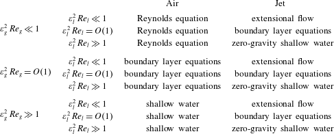
The resulting models can be split into nine regimes depending on the sizes of the reduced Reynolds numbers in each fluid. It should be noted that, in each regime, we shall consider the distinguished limit that retains as many physical effects as possible. We discuss the resulting assumptions later in this section. We summarise these regimes in this section before moving on to derive the corresponding leading-order equations of motion in § 4.
(i) When the reduced Reynolds number in the air layer is small, that is
 $\unicode[STIX]{x1D700}_{g}^{2}Re_{g}\ll 1$
, the appropriate air pressure scale is found by balancing the pressure gradient and viscous stress terms in the horizontal momentum equation (2.4), and is therefore given by (3.1)so that$$\begin{eqnarray}{\mathcal{P}}_{g}=\frac{\unicode[STIX]{x1D707}_{g}U_{s}}{\unicode[STIX]{x1D700}_{g}^{2}L},\end{eqnarray}$$
${\mathcal{Q}}=1$
. The length scale
$L$
over which we see pressure-driven deflections of the jet is then found by setting
$\unicode[STIX]{x1D706}=1$
in (2.17), so that (3.2)We shall call$$\begin{eqnarray}L=L_{v}\equiv \left(\frac{\unicode[STIX]{x1D70C}_{l}U_{s}\ell _{l}^{2}\ell _{g}^{2}}{\unicode[STIX]{x1D707}_{g}}\right)^{1/3}.\end{eqnarray}$$
$L_{v}$
the deflection length scale for a viscous air layer. With this choice of
$L$
, the air flow will be governed at leading order by the Reynolds lubrication equation (see below).
(ii) If the reduced Reynolds number in the air layer is
$O(1)$
, the air pressure scale is still given by (3.1), so that (3.2) is still the appropriate horizontal length scale. However, in this regime, the air flow is governed by the unsteady boundary layer equations, which are coupled with the jet flow. While this regime is certainly of interest, we shall not consider it in any further detail in this paper.(iii) If the reduced Reynolds number in the air is large, the air pressure scale is instead chosen by balancing the pressure gradient and inertial terms in the horizontal momentum equation (2.4), and is therefore given by
(3.3)so that$$\begin{eqnarray}{\mathcal{P}}_{g}=\unicode[STIX]{x1D70C}_{g}U_{s}^{2},\end{eqnarray}$$
${\mathcal{Q}}=\unicode[STIX]{x1D700}_{g}^{2}\,Re_{g}\gg 1$
. Whence,
$\unicode[STIX]{x1D706}=1$
if we take the length scale
$L$
to be given by (3.4)where$$\begin{eqnarray}L=L_{i}\equiv \frac{\ell _{l}}{\unicode[STIX]{x1D70C}^{1/2}},\end{eqnarray}$$
$\unicode[STIX]{x1D70C}=\unicode[STIX]{x1D70C}_{g}/\unicode[STIX]{x1D70C}_{l}$
. We shall call
$L_{i}$
the deflection length scale for an inviscid air layer. Under the additional assumption that the flow in the air is irrotational, the leading-order equations of motion for the air layer are given by the shallow-water equations (see below).


The jet flow in each of these asymptotic regimes depends on the size of the reduced Reynolds number in the liquid. When
 $\unicode[STIX]{x1D700}_{l}^{2}\,Re_{l}\ll 1$
, the flow in the jet is extensional at leading order, akin to the flow in viscous fibres (see, for example, Trouton Reference Trouton1906). If
 $\unicode[STIX]{x1D700}_{l}^{2}\,Re_{l}=O(1)$
, the jet is governed by the unsteady boundary layer equations; again, this is an interesting regime, but we do not consider it any further here. Finally, when
 $\unicode[STIX]{x1D700}_{l}^{2}\,Re_{l}\gg 1$
, if we make the additional assumption that the liquid flow is irrotational, the zero-gravity shallow-water equations hold in the jet, akin to the splash jets in classical Wagner theory; see, for example, Howison et al. (Reference Howison, Ockendon and Wilson1991).
Returning to the remaining parameters in our model, we assume that the viscosity and density ratios are small, namely
 $0<\unicode[STIX]{x1D707}$
,
 $\unicode[STIX]{x1D70C}\ll 1$
. Furthermore, so that gravity and surface tension affect the centreline of the jet, but not its thickness to leading order, we assume that
 $$\begin{eqnarray}{\mathcal{F}}=\frac{1}{\unicode[STIX]{x1D700}_{l}\,\mathit{Fr}^{2}}=O(1),\quad \unicode[STIX]{x1D6FE}=\frac{2}{\unicode[STIX]{x1D700}_{l}\,\mathit{We}}=O(1).\end{eqnarray}$$
We now return to our assumption that the flow in the air above the jet can be neglected. The leading-order contribution to the jet motion due to the upper air would be through the tangential stress boundary condition, equation (2.18). The jet motion would induce a boundary layer in the upper air region at the free surface of the jet, and this boundary layer would produce a shear of
 $O(\unicode[STIX]{x1D707}\sqrt{\mathit{Re }_{g}})$
on the jet. Hence, in each regime we have discussed above, this shear can be neglected provided that
 $$\begin{eqnarray}\unicode[STIX]{x1D707}=o\left(\frac{\unicode[STIX]{x1D700}_{l}^{2}}{\unicode[STIX]{x1D70C}\,\mathit{Re}_{l}}\right).\end{eqnarray}$$
If we are in a regime in which
 $L$
is given by the deflection length scale for a viscous air layer, (3.2), we are already assuming that
 $\unicode[STIX]{x1D707}=O(\unicode[STIX]{x1D700}_{l}^{2}\unicode[STIX]{x1D700}_{g}^{2}\,\mathit{Re}_{l})$
, so that (3.6) reduces to
 $\unicode[STIX]{x1D70C}\ll 1/(\unicode[STIX]{x1D702}^{2}\unicode[STIX]{x1D700}_{l}^{2}\,\mathit{Re}_{l})$
. Therefore, neglecting the shear stress is reasonable for
 $\unicode[STIX]{x1D700}_{l}^{2}\,\mathit{Re}_{l}=O(1)$
, but introduces a slightly stricter limit on the density ratio when the
 $\unicode[STIX]{x1D700}_{l}^{2}\,\mathit{Re}_{l}\gg 1$
. If we are in a regime in which
 $L$
is given by the deflection length scale for an inviscid air layer, equation (3.4), we require
 $\unicode[STIX]{x1D70C}=O(\unicode[STIX]{x1D700}_{l}^{2})$
, so that (3.6) reduces to
 $\unicode[STIX]{x1D707}\ll 1/\mathit{Re}_{l}$
, which only adds an additional restriction on the viscosity ratio if
 $\mathit{Re}_{l}\gg 1$
.
In summary, we depict the nine asymptotic regimes in table 1. We shall, in particular, concentrate on the four asymptotic limits in which
 $\unicode[STIX]{x1D700}_{i}^{2}\,Re_{i}$
are large or small for
 $i=g,l$
. We shall discuss the relevance and applicability of the predictions for
 $L$
given by (3.2) and (3.4) in § 7.1.
The leading-order governing equations in each of the nine asymptotic regimes based on the sizes of the reduced Reynolds numbers in either fluid when both
 $\unicode[STIX]{x1D700}_{l},\unicode[STIX]{x1D700}_{g}\ll 1$
and
 $\unicode[STIX]{x1D702}=O(1)$
.

4 Governing equations
We shall now outline the leading-order governing equations in four of the asymptotic regimes discussed in the previous section.
4.1 Viscous air, viscous liquid
When the reduced Reynolds number in each fluid is small, the air pressure scale is given by (3.1) and the appropriate horizontal length scale is given by (3.2). Much of the following analysis follows that for viscous fibres, as described by Howell (Reference Howell1994), van de Fliert et al. (Reference van de Fliert, Howell and Ockendon1995) and Howell (Reference Howell1996). To derive the most general possible model, we shall assume that
 $\mathit{Re}_{l}$
and
 $\mathit{Re}_{g}$
are of order unity. We expand all of the independent variables in powers of
 $\unicode[STIX]{x1D700}_{l}^{2}$
– this is without loss of generality, since we have assumed that
 $\unicode[STIX]{x1D702}=O(1)$
.
In the jet, the leading-order form of the Navier–Stokes equations (2.1)–(2.3) subject to the stress conditions on the upper and lower free surfaces (2.14), (2.15), (2.18) and (2.19) allows us to deduce that, to leading order, the horizontal component of velocity and the pressure do not vary across the jet, since it is thin. Thus,
 $u=u(x,t)$
and
 $p=-(2/\mathit{Re}_{l})u_{x}$
at leading order. Utilisation of (2.3) along with the leading-order versions of the kinematic conditions (2.11) and (2.12) allows us to deduce the usual conservation of mass equation
 $$\begin{eqnarray}h_{t}+(uh)_{x}=0.\end{eqnarray}$$
In the air layer, the leading-order form of the Navier–Stokes equations (2.4)–(2.6) subject to the no-slip, no-flux condition on the substrate (2.9), the kinematic condition (2.10) and the continuity of velocity condition (2.13a ) leads to the lubrication equation,
 $$\begin{eqnarray}H_{t}+\left(\frac{uH}{2}-\frac{H^{3}P_{x}}{12}\right)_{x}=0,\end{eqnarray}$$
where, to leading order,
 $P=P(x,t)$
. We can clearly see both the Couette and the Poiseuille parts of the flow in (4.2).
We can now integrate the
 $O(\unicode[STIX]{x1D700}_{l}^{2})$
version of the horizontal momentum equation (2.1) across the jet and apply the shear stress conditions (2.18) and (2.19) to deduce that
 $$\begin{eqnarray}h(u_{t}+uu_{x})=\frac{4}{\mathit{Re}_{l}}(hu_{x})_{x}.\end{eqnarray}$$
The term on the right-hand side is the Trouton term seen in extensional flow models for viscous fibres. To close the system, we integrate the
 $O(\unicode[STIX]{x1D700}_{l}^{2})$
version of the vertical momentum equation (2.2) across the jet and apply the normal stress conditions (2.14) and (2.15). The algebraic details are presented in appendix B, yielding
 $$\begin{eqnarray}\displaystyle \unicode[STIX]{x1D702}h\left[\left(u^{2}-\frac{4u_{x}}{\mathit{Re}_{l}}-\frac{\unicode[STIX]{x1D6FE}}{h}\right)H_{xx}+2uH_{xt}+H_{tt}\right] & = & \displaystyle P-h{\mathcal{F}}+\frac{\unicode[STIX]{x1D6FE}}{2}h_{xx}-h^{2}u_{x}^{2}\nonumber\\ \displaystyle & & \displaystyle +\,\frac{2}{\mathit{Re}_{l}}(2h(h_{x}u_{x})_{x}+h^{2}u_{xxx}).\qquad\end{eqnarray}$$
We note that by writing
 $\unicode[STIX]{x1D702}H=H_{c}-h/2$
, where
 $H_{c}$
is the centreline of the jet, we can reduce (4.4) to the inertial centreline equation for the stretching of a two-dimensional viscous sheet, as given by (94) in Howell (Reference Howell1996), with the addition of the air pressure term,
 $P(x,t)$
. We shall continue to use
 $H$
and
 $h$
in our analysis, since the thickness of the air layer is most frequently what we are interested in.
In summary, in the viscous jet/viscous air regime, the leading-order model for the horizontal component of the jet velocity,
 $u(x,t)$
, the jet thickness,
 $h(x,t)$
, the air layer thickness,
 $H(x,t)$
, and the air pressure,
 $P(x,t)$
, is given by the extensional flow equations (4.1) and (4.3) in the jet coupled with the lubrication equation in the air layer, (4.2), with the centreline deflection determined from the pressure-jump equation, (4.4). The length scale over which we see such a deflection is given by the deflection length scale for a viscous air layer, (3.2).
4.2 Viscous air, inviscid liquid
In the limit in which the reduced Reynolds number is large in the jet and small in the air, we can make progress under the additional assumption that the flow is irrotational in the jet, as in Wagner theory. The pressure scale in the air is still given by (3.1), so that the appropriate length scale is again given by (3.2). On expanding the variables in asymptotic series in powers of
 $\unicode[STIX]{x1D700}_{l}^{2}$
, a similar analysis to § 4.1 reveals that, at leading order,
 $u(x,t)$
,
 $h(x,t)$
,
 $H(x,t)$
and
 $P(x,t)$
, satisfy
 $$\begin{eqnarray}\displaystyle & h_{t}+(uh)_{x}=0, & \displaystyle\end{eqnarray}$$
 $$\begin{eqnarray}\displaystyle & u_{t}+uu_{x}=0, & \displaystyle\end{eqnarray}$$
 $$\begin{eqnarray}\displaystyle & \displaystyle H_{t}+\left(\frac{uH}{2}-\frac{H^{3}P_{x}}{12}\right)_{x}=0, & \displaystyle\end{eqnarray}$$
 $$\begin{eqnarray}\displaystyle & \displaystyle \unicode[STIX]{x1D702}h\left[\left(u^{2}-\frac{\unicode[STIX]{x1D6FE}}{h}\right)H_{xx}+2uH_{xt}+H_{tt}\right]=P-h{\mathcal{F}}+\frac{\unicode[STIX]{x1D6FE}}{2}h_{xx}-h^{2}u_{x}^{2}. & \displaystyle\end{eqnarray}$$
Here, we note that (4.5) and (4.6) are the usual Wagner jet equations; see, for example, Howison et al. (Reference Howison, Ockendon and Wilson1991) and Riboux & Gordillo (Reference Riboux and Gordillo2015).
4.3 Inviscid air, viscous liquid
If the reduced Reynolds number is small in the jet, but large in the air, we can make progress under the additional assumption that the flow in the air is irrotational (thus assuming that there is no separation of viscous boundary layers on the time scale under consideration). The air pressure scale is now given by (3.3), so that the appropriate horizontal length scale is defined by the deflection length scale for an inviscid air layer, equation (3.4). Proceeding as in § 4.1, the leading-order problem for
 $u(x,t)$
,
 $h(x,t)$
,
 $H(x,t)$
,
 $P(x,t)$
and the horizontal component of the air velocity,
 $U(x,t)$
, is found to be given by
 $$\begin{eqnarray}\displaystyle & h_{t}+(uh)_{x}=0, & \displaystyle\end{eqnarray}$$
 $$\begin{eqnarray}\displaystyle & \displaystyle h(u_{t}+uu_{x})=\frac{4}{\mathit{Re}_{l}}(hu_{x})_{x}, & \displaystyle\end{eqnarray}$$
 $$\begin{eqnarray}\displaystyle & U_{t}+UU_{x}=-P_{x}, & \displaystyle\end{eqnarray}$$
 $$\begin{eqnarray}\displaystyle & H_{t}+(UH)_{x}=0, & \displaystyle\end{eqnarray}$$
 $$\begin{eqnarray}\displaystyle & & \displaystyle \displaystyle \unicode[STIX]{x1D702}h\left[\left(u^{2}-\frac{4u_{x}}{\mathit{Re}_{l}}-\frac{\unicode[STIX]{x1D6FE}}{h}\right)H_{xx}+2uH_{xt}+H_{tt}\right]\nonumber\\ \displaystyle & & \displaystyle \quad =P-h{\mathcal{F}}+\frac{\unicode[STIX]{x1D6FE}}{2}h_{xx}-h^{2}u_{x}^{2}+\frac{2}{\mathit{Re}_{l}}(2h(h_{x}u_{x})_{x}+h^{2}u_{xxx}).\end{eqnarray}$$
4.4 Inviscid air, inviscid liquid
Finally, in the limit in which the reduced Reynolds number is large in both the air and the jet, we assume that both flows are irrotational and proceed as in the previous sections. The pressure scale and appropriate horizontal length scale are given by (3.3) and (3.4) respectively. The leading-order problem for
 $u(x,t)$
,
 $h(x,t)$
,
 $H(x,t)$
,
 $U(x,t)$
and
 $P(x,t)$
is given by
 $$\begin{eqnarray}\displaystyle & h_{t}+(uh)_{x}=0, & \displaystyle\end{eqnarray}$$
 $$\begin{eqnarray}\displaystyle & u_{t}+uu_{x}=0, & \displaystyle\end{eqnarray}$$
 $$\begin{eqnarray}\displaystyle & U_{t}+UU_{x}=-P_{x}, & \displaystyle\end{eqnarray}$$
 $$\begin{eqnarray}\displaystyle & H_{t}+(UH)_{x}=0, & \displaystyle\end{eqnarray}$$
 $$\begin{eqnarray}\displaystyle & \displaystyle \unicode[STIX]{x1D702}h\left[\left(u^{2}-\frac{\unicode[STIX]{x1D6FE}}{h}\right)H_{xx}+2uH_{xt}+H_{tt}\right]=P-h{\mathcal{F}}+\frac{\unicode[STIX]{x1D6FE}}{2}h_{xx}-h^{2}u_{x}^{2}. & \displaystyle\end{eqnarray}$$
4.5 Summary
We have outlined the derivation of the equations governing the motion of a thin jet above a thin air layer in four different asymptotic regimes. Although we have derived these equations in the context of an infinite jet, they are equally relevant along the bulk of a long but finite jet, provided that the length of the jet is comparable to the appropriate deflection length scales given in (3.2) and (3.4). In these latter instances, appropriate boundary and initial conditions will need to be specified, which is non-trivial since the equations are highly nonlinear. We shall discuss this in more detail in § 6.1.
It is perhaps worth reiterating that we have considered the particular distinguished limit in which the air pressure jump, surface tension and gravity influence the centreline deflection, but have no effect on the jet thickness or horizontal component of velocity at leading order. Thus, in each of §§ 4.1–4.4, the jet flow equations decouple from the air flow equations and centreline equation. Hence, in order to put our model in context, we discuss how our analysis could be used to extend the model for a detached lamella in Riboux & Gordillo (Reference Riboux and Gordillo2015). First, we could find the horizontal component of the jet velocity and the jet thickness by solving (4.1), (4.3) or (4.5), (4.6) subject to appropriate jet-root boundary conditions, for example the Wagner jet-root conditions modified to account for local viscous effects, as in Riboux & Gordillo (Reference Riboux and Gordillo2015). In principle, we could then use
 $u$
and
 $h$
to solve (4.2), (4.4) or (4.7), (4.8) subject to appropriate boundary conditions for the motion of the jet centreline under the action of the air-cushioning layer; the effect of the latter is not considered by Riboux & Gordillo (Reference Riboux and Gordillo2015). We discuss the relevance of our assumptions on the importance of surface tension and gravity by considering experiments in several studies in § 7.1. It is certainly possible to consider other distinguished limits, for example regimes where surface tension plays a more important role, which we discuss in appendix A.
5 Linear stability analysis
Whether the liquid jet is dominated by viscous forces, so that the extensional flow equations (4.1), (4.3) hold, or by inviscid forces, so that the zero-gravity shallow-water equations (4.5), (4.6) hold,
 $h=1$
,
 $u=1$
(without loss of generality) is a spatially uniform steady-state solution on an unbounded domain. Remarkably, looking at the numerical simulations of Thoraval et al. (Reference Thoraval, Takehara, Etoh, Popinet, Ray, Josserand, Zaleski and Thoroddsen2012), even for a finite jet, aside from a region near the tip where surface tension dominates, a constant-thickness, constant-velocity jet appears to be a reasonable working approximation to their simulations.
In this section, we aim to show that a constant-thickness, constant-velocity jet becomes unstable to small perturbations to its centreline and the pressure in the air below the jet, providing a possible mechanism for the onset of motion leading to bubble entrapment, seen in, for example, Thoroddsen et al. (Reference Thoroddsen, Takehara and Etoh2010) and Thoraval et al. (Reference Thoraval, Takehara, Etoh and Thoroddsen2013), and jet bending. Since we are looking for instabilities of the jet centreline (effectively
 $H$
) rather than the jet thickness, we are studying jet bending as opposed to jet disintegration. Indeed, since the jet and air flows decouple in each of the regimes §§ 4.1–4.4, we can consider briefly the linear stability of (4.1) and (4.3) by setting
 $$\begin{eqnarray}(u,h)=1+\unicode[STIX]{x1D6FF}(u_{1},h_{1})\text{e}^{\text{i}(kx-\unicode[STIX]{x1D6FA}t)},\end{eqnarray}$$
where
 $\unicode[STIX]{x1D6FF}\ll 1$
measures the size of the perturbation, the wavenumber
 $k$
is assumed to be real and positive without loss of generality and
 $\unicode[STIX]{x1D6FA}$
is the frequency. We have instability if
 $\text{Im}(\unicode[STIX]{x1D6FA})>0$
. A regular perturbation analysis yields in the usual way the dispersion relation
 $$\begin{eqnarray}\unicode[STIX]{x1D6FA}=k-\frac{4\text{i}k^{2}}{\mathit{Re}_{l}},\end{eqnarray}$$
which shows that infinitesimal perturbations to the jet thickness and velocity are linearly stable (when
 $\mathit{Re}_{l}$
is finite) or neutrally stable (when
 $\mathit{Re}_{l}=\infty$
) in this regime.
Hence, as we shall go on to see, jet bending occurs before jet disintegration in each of the regimes in §§ 4.1–4.4. We shall separate our analysis into two sections depending on whether the air layer is dominated by viscous or inertial forces. It should be noted that, under the assumption that
 $u$
and
 $h$
are constant, the jet Reynolds number does not enter the linear stability analysis.
5.1 Viscous air layer
When
 $u=1$
and
 $h=1$
, the Reynolds lubrication equation (4.2) and the centreline deflection equation (4.4) reduce to
 $$\begin{eqnarray}H_{t}+\left(\frac{H}{2}-\frac{H^{3}P_{x}}{12}\right)_{x}=0,\quad \unicode[STIX]{x1D702}[(1-\unicode[STIX]{x1D6FE})H_{xx}+2H_{xt}+H_{tt}]=P-{\mathcal{F}}.\end{eqnarray}$$
There is a spatially uniform solution of (5.3) given by
 $$\begin{eqnarray}H=1,\quad P={\mathcal{F}},\end{eqnarray}$$
where we take the constant solution for the thickness of the air layer to be unity without loss of generality. We seek a dispersion relation between the frequency,
 $\unicode[STIX]{x1D714}$
, and the wavenumber,
 $k$
, by expanding in the usual way via
 $$\begin{eqnarray}(H,P)=(1,{\mathcal{F}})+\unicode[STIX]{x1D6FF}(H_{1},P_{1})\text{e}^{\text{i}(kx-\unicode[STIX]{x1D714}t)},\end{eqnarray}$$
where
 $\unicode[STIX]{x1D6FF}\ll 1$
. On substituting (5.5) into (5.3), we deduce from the linearised problem (at
 $O(\unicode[STIX]{x1D6FF})$
) that
 $\unicode[STIX]{x1D714}$
must satisfy the quadratic
 $$\begin{eqnarray}-\text{i}\unicode[STIX]{x1D714}+\frac{\text{i}k}{2}-\unicode[STIX]{x1D6E4}((1-\unicode[STIX]{x1D6FE})k^{4}-2k^{3}\unicode[STIX]{x1D714}+\unicode[STIX]{x1D714}^{2}k^{2})=0,\end{eqnarray}$$
where
 $\unicode[STIX]{x1D6E4}=\unicode[STIX]{x1D702}/12$
. We find that the two roots of this dispersion relation are given by
 $$\begin{eqnarray}\unicode[STIX]{x1D714}_{\pm }=k-\frac{\text{i}}{2\unicode[STIX]{x1D6E4}k^{2}}\left(-1\pm \sqrt{1-4(a-b\text{i})}\right),\quad \text{where}~a=\unicode[STIX]{x1D6E4}^{2}\unicode[STIX]{x1D6FE}k^{6},b=\frac{\unicode[STIX]{x1D6E4}k^{3}}{2}\end{eqnarray}$$
and the principal branch of the square root is taken. It is trivial to note that
 $a,b>0$
for all
 $k>0$
.
The imaginary part of (5.7) dictates the growth rate of the infinitesimal disturbances: we find that
 $$\begin{eqnarray}\text{Im}(\unicode[STIX]{x1D714}_{\pm })=\frac{1}{2\unicode[STIX]{x1D6E4}k^{2}}\left(-1\pm \left(\frac{(1-4a)+\sqrt{(1-4a)^{2}+16b^{2}}}{2}\right)^{1/2}\right).\end{eqnarray}$$
For an instability in either branch, we require
 $\text{Im}(\unicode[STIX]{x1D714}_{\pm })>0$
. Since the term
 $(1-4a)^{2}+16b^{2}$
is always positive,
 $\text{Im}(\unicode[STIX]{x1D714}_{-})<0$
for all
 $k$
, so that we can only get instability if
 $\text{Im}(\unicode[STIX]{x1D714}_{+})>0$
. This only occurs when
 $b^{2}>a$
or
 $$\begin{eqnarray}\unicode[STIX]{x1D6FE}=\frac{2}{\unicode[STIX]{x1D700}_{l}\,\mathit{We}}<\frac{1}{4}.\end{eqnarray}$$
It is interesting to note that this requirement is independent of
 $k$
; hence, if
 $\unicode[STIX]{x1D6FE}$
satisfies (5.9), then the positive branch of the dispersion relation is unstable for all wavenumbers
 $k>0$
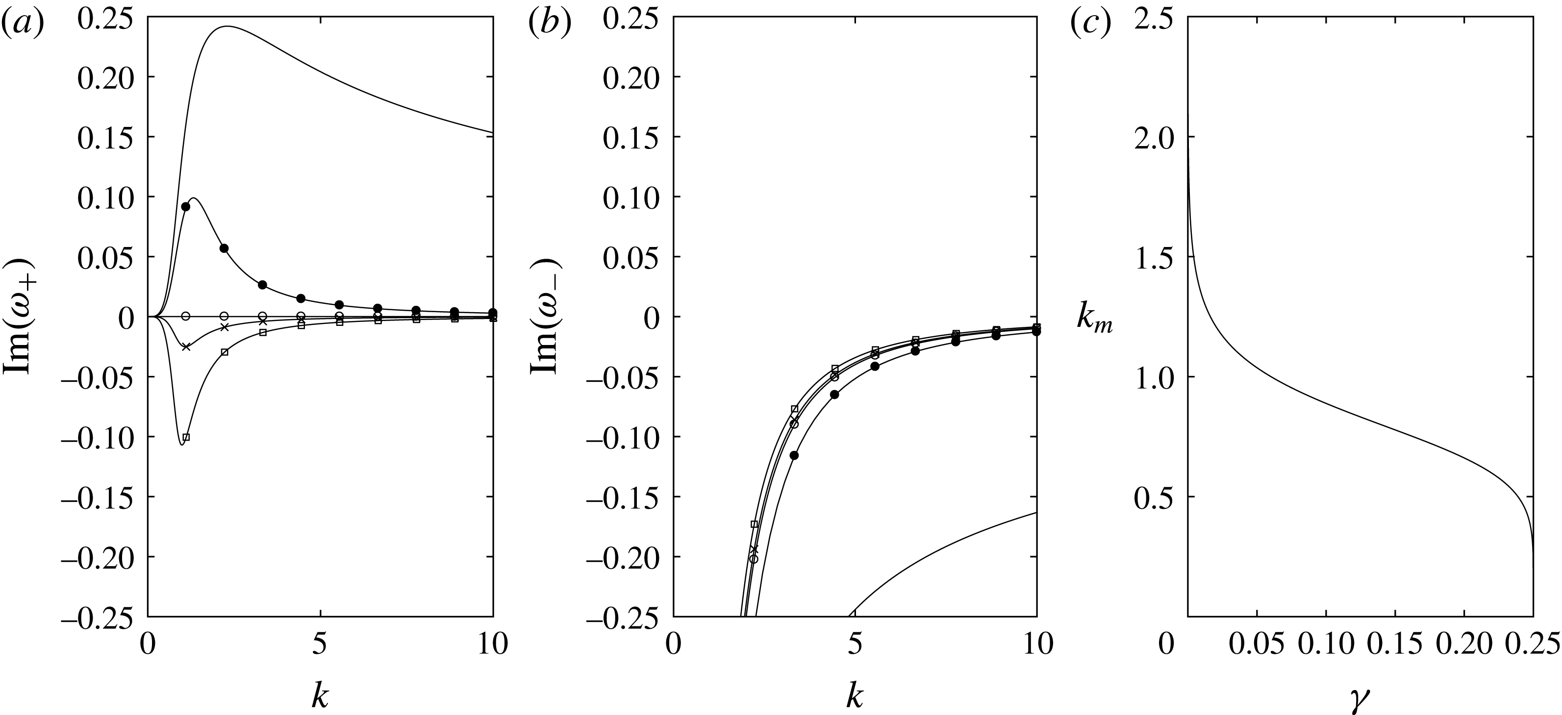
. We plot
 $\text{Im}(\unicode[STIX]{x1D714}_{\pm })$
with
 $\unicode[STIX]{x1D6E4}=1$
for various values of
 $\unicode[STIX]{x1D6FE}$
in figure 6(a,b), which illustrates that, as we decrease the Weber number – increasing
 $\unicode[STIX]{x1D6FE}$
– we see three different behaviours in
 $\text{Im}(\unicode[STIX]{x1D714}_{+})$
, while there is no qualitative change in the behaviour of
 $\text{Im}(\unicode[STIX]{x1D714}_{-})$
. From (5.9), we know that the critical value at which we see a change in stability is given by
 $\unicode[STIX]{x1D6FE}=1/4$
. For
 $\unicode[STIX]{x1D6FE}<1/4$
, that is for sufficiently small surface tension, perturbations are linearly unstable to all wavenumbers
 $k>0$
, with the growth rate for short wavelengths decaying like
 $$\begin{eqnarray}\text{Im}(\unicode[STIX]{x1D714}_{+})\sim \frac{1}{2\unicode[STIX]{x1D6E4}}\left(-1+\sqrt{\frac{1}{4\unicode[STIX]{x1D6FE}}}\right)\frac{1}{k^{2}}\quad \text{as}~k\rightarrow \infty .\end{eqnarray}$$
When
 $\unicode[STIX]{x1D6FE}=1/4$
,
 $\text{Im}(\unicode[STIX]{x1D714}_{+})$
is identically zero for all
 $k>0$
, and hence this branch is neutrally stable. For
 $\unicode[STIX]{x1D6FE}>1/4$
, we note that
 $\text{Im}(\unicode[STIX]{x1D714}_{+})<0$
for all
 $k>0$
, so that we have linear stability for all wavenumbers.
(a,b) Dispersion relation branches with
 $\unicode[STIX]{x1D6E4}=1$
for various values of the inverse Weber number:
 $\unicode[STIX]{x1D6FE}=0$
(solid line),
 $\unicode[STIX]{x1D6FE}=1/10$
(filled circles),
 $\unicode[STIX]{x1D6FE}=1/4$
(circles),
 $\unicode[STIX]{x1D6FE}=3/10$
(crosses) and
 $\unicode[STIX]{x1D6FE}=1/2$
(squares). (c) The wavenumber of the most unstable mode,
 $k_{m}$
, as a function of
 $\unicode[STIX]{x1D6FE}$
with
 $\unicode[STIX]{x1D6E4}=1$
.

To facilitate comparisons with experiments and simulations, we wish to discern the most unstable mode; that is, the wavenumber
 $k$
that maximises
 $\text{Im}(\unicode[STIX]{x1D714}_{+})$
. We find that the dimensionless wavenumber of the most unstable mode,
 $k_{m}$
, is given by
 $$\begin{eqnarray}k_{m}=\frac{1}{\unicode[STIX]{x1D6E4}^{1/3}}(v^{2}(v^{2}-1))^{1/6},\end{eqnarray}$$
where
 $v$
is the unique positive root of the sextic
 $$\begin{eqnarray}0=4\unicode[STIX]{x1D6FE}v^{4}(3v^{2}+3v-2)+v^{2}-3v-2.\end{eqnarray}$$
If we fix
 $\unicode[STIX]{x1D6E4}=1$
, we can investigate the effect of
 $\unicode[STIX]{x1D6FE}$
on
 $k_{m}$
, and we plot the result in figure 6(c). As
 $\unicode[STIX]{x1D6FE}$
increases, so too does the wavelength of the most unstable mode.
If we fix
 $\unicode[STIX]{x1D6FE}$
,
 $k_{m}$
is inversely proportional to the cubic root of
 $\unicode[STIX]{x1D6E4}$
. Therefore, increasing
 $\unicode[STIX]{x1D6E4}$
increases the wavelength of the most unstable mode. Since
 $$\begin{eqnarray}\unicode[STIX]{x1D6E4}=\frac{\unicode[STIX]{x1D702}}{12}=\frac{\ell _{g}}{12\ell _{l}},\end{eqnarray}$$
if we decrease the thickness of the liquid jet or increase the thickness of the air layer, we increase the wavelength of the most unstable mode. We note that as
 $k_{m}$
decreases,
 $\text{Im}(\unicode[STIX]{x1D714}_{+}(k_{m}))$
decreases, so that the growth rate is reduced.
5.2 Inviscid air layer
In the inviscid air regime, we perform a similar linear stability analysis of the centreline deflection equations (4.16)–(4.18) with
 $u=h=1$
to that in § 5.1 with the additional assumption that the air has a constant tangential speed in the base state, which we denote by
 $U_{0}$
. By perturbing about the spatially uniform steady-state solution by setting
 $$\begin{eqnarray}(H,U,P)=(1,U_{0},{\mathcal{F}})+\unicode[STIX]{x1D6FF}(H_{1},U_{1},P_{1})\text{e}^{\text{i}(kx-\unicode[STIX]{x1D714}t)},\end{eqnarray}$$
where
 $\unicode[STIX]{x1D6FF}\ll 1$
, we find that the dispersion relation in the inviscid air regime is given by
 $$\begin{eqnarray}0=(\unicode[STIX]{x1D702}k^{2}+1)\unicode[STIX]{x1D714}^{2}-2k(\unicode[STIX]{x1D702}k^{2}+U_{0})\unicode[STIX]{x1D714}+\unicode[STIX]{x1D702}(1-\unicode[STIX]{x1D6FE})k^{4}+U_{0}^{2}k^{2},\end{eqnarray}$$
giving the two roots
 $$\begin{eqnarray}\unicode[STIX]{x1D714}_{\pm }=\frac{k}{1+\unicode[STIX]{x1D702}k^{2}}(U_{0}+\unicode[STIX]{x1D702}k^{2}\pm k\sqrt{\unicode[STIX]{x1D6FE}\unicode[STIX]{x1D702}(1+\unicode[STIX]{x1D702}k^{2})-\unicode[STIX]{x1D702}(U_{0}-1)^{2}}).\end{eqnarray}$$
Again, we require
 $\text{Im}(\unicode[STIX]{x1D714}_{\pm })>0$
for instability.
If
 $U_{0}=1$
, that is if the unperturbed air velocity is the same as the jet velocity, the disturbance is neutrally stable, which is in agreement with Tammisola et al. (Reference Tammisola, Sasaki, Lundell, Matsubara and Söderberg2011), who show that a co-flowing gas can stabilise a liquid jet provided that the difference between the mean gas and jet speeds is sufficiently small.
If
 $U_{0}\neq 1$
, we can find a range of unstable wavenumbers provided that the surface-tension parameter,
 $\unicode[STIX]{x1D6FE}$
, is sufficiently small. Considering (5.16), if
 $0<\unicode[STIX]{x1D6FE}<(U_{0}-1)^{2}$
, the range of unstable wavenumbers is
 $$\begin{eqnarray}0<k<\sqrt{\frac{1}{\unicode[STIX]{x1D702}\unicode[STIX]{x1D6FE}}((U_{0}-1)^{2}-\unicode[STIX]{x1D6FE})}.\end{eqnarray}$$
If
 $\unicode[STIX]{x1D6FE}>(U_{0}-1)^{2}$
, we have neutral stability. Thus, we identify
 $\unicode[STIX]{x1D6FE}_{c}=(U_{0}-1)^{2}$
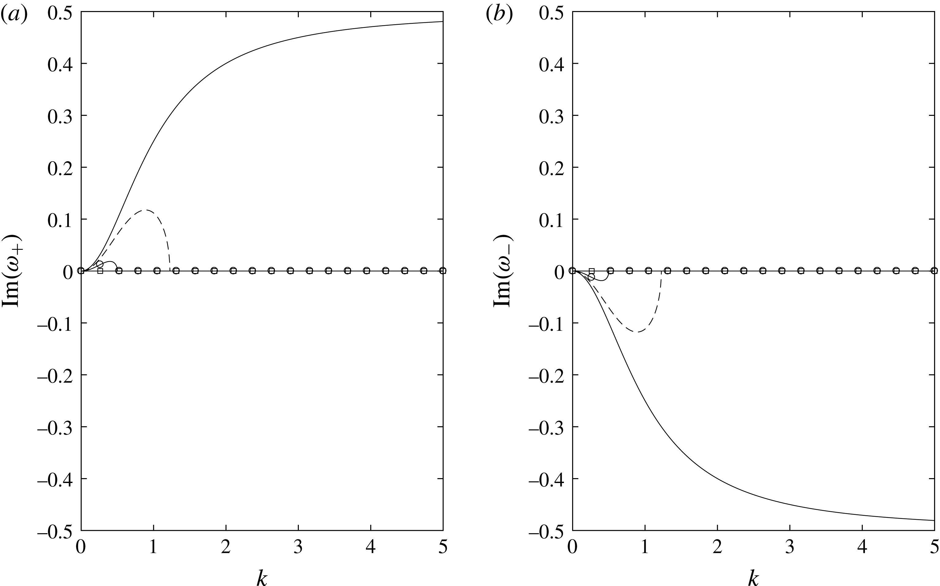
as the critical value of the surface-tension parameter. We plot
 $\text{Im}(\unicode[STIX]{x1D714}_{\pm })$
for
 $\unicode[STIX]{x1D702}=1$
and
 $U_{0}=1/2$
for various values of
 $\unicode[STIX]{x1D6FE}$
in figure 7. We find that, when
 $0<\unicode[STIX]{x1D6FE}<\unicode[STIX]{x1D6FE}_{c}$
, the most unstable wavenumber is given by
 $$\begin{eqnarray}k_{m}=\left(\frac{1}{2\unicode[STIX]{x1D702}}\left(-3+\sqrt{1+\frac{8}{\unicode[STIX]{x1D6FE}}(U_{0}-1)^{2}}\right)\right)^{1/2}.\end{eqnarray}$$
It should be noted that
 $k_{m}\rightarrow 0$
as
 $\unicode[STIX]{x1D6FE}\rightarrow \unicode[STIX]{x1D6FE}_{c}$
. Furthermore, it should be noted that as
 $\unicode[STIX]{x1D6FE}\rightarrow 0$
, the range of unstable wavenumbers gets larger; indeed, if
 $\unicode[STIX]{x1D6FE}=0$
, the jet is unstable to disturbances of all wavelengths. Nevertheless, the growth rate is bounded for arbitrarily short wavelengths in the zero-surface-tension case, with
 $$\begin{eqnarray}\text{Im}(\unicode[STIX]{x1D714}_{+})\sim \sqrt{\frac{1}{\unicode[STIX]{x1D702}}}(U_{0}-1)-\left(\frac{1}{\unicode[STIX]{x1D702}}\right)^{3/2}\frac{U_{0}-1}{k^{2}}+\cdots \quad \text{as}~k\rightarrow \infty .\end{eqnarray}$$
Branches of the dispersion relation for fixed
 $\unicode[STIX]{x1D706}=1$
,
 $\unicode[STIX]{x1D702}=1$
and
 $U_{0}=1/2$
for various values of the inverse Weber number:
 $\unicode[STIX]{x1D6FE}=0$
(solid line),
 $\unicode[STIX]{x1D6FE}=0.1$
(dashed line),
 $\unicode[STIX]{x1D6FE}=0.2$
(circles),
 $\unicode[STIX]{x1D6FE}=0.25$
(squares). It should be noted that
 $\unicode[STIX]{x1D6FE}_{c}=1/4$
for this particular example.

5.3 Discussion
The linear stability analysis indicates that the models derived in §§ 3–4 are sensitive to perturbations to the jet centreline or the air pressure in the cushioning layer. We consider it instructive to consider (5.11), (5.12) and (5.18) in comparison with the bubble rings observed in experiments in Thoraval et al. (Reference Thoraval, Takehara, Etoh and Thoroddsen2013), although any comparisons with experimental observations can only be qualitative due to the fact that liquid–liquid impacts are considered therein.
In Thoraval et al. (Reference Thoraval, Takehara, Etoh and Thoroddsen2013), the authors note that rings of air are entrapped by the advancing ejecta as a water droplet impacts a pool of the same fluid. The average radial spacing of the rings in figure 4(f) of that paper is approximately
 $26~\unicode[STIX]{x03BC}\text{m}$
. In that experiment,
 $\unicode[STIX]{x1D70C}_{l}=10^{3}~\text{kg}~\text{m}^{-3}$
,
 $\unicode[STIX]{x1D70C}_{g}=1~\text{kg}~\text{m}^{-3}$
,
 $\unicode[STIX]{x1D707}_{l}=10^{-3}$
Pa s,
 $\unicode[STIX]{x1D707}_{g}=1.81\times 10^{-3}$
Pa s and
 $\unicode[STIX]{x1D70E}=7.2\times 10^{-2}~\text{N}~\text{m}^{-1}$
. The typical jet velocity is estimated to be close to the tip velocity,
 $20.5~\text{m}~\text{s}^{-1}$
, while the ejecta thickness is estimated using the scaling
 $\sqrt{\unicode[STIX]{x1D708}_{l}t^{\ast }}\approx 4.1\times 10^{-6}$
m derived in Josserand & Zaleski (Reference Josserand and Zaleski2003). It should be noted that in this configuration, since the centreline of the ejecta follows a curved trajectory (cf. figure 11 in that paper), the thin air layer is in fact that trapped between the ejecta and the upper bulk of the droplet. Since it is not possible to get a reliable estimate for the thickness,
 $\ell _{g}$
, of this layer, we calculate the values of
 $\ell _{g}$
that would lead to the reported dominant wavelength of
 $26~\unicode[STIX]{x03BC}\text{m}$
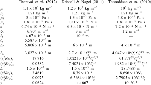
in each of our regimes, and determine that the most reasonable regime is the viscous air limit. Using the above figures,
 $L_{v}\approx 1.75\times 10^{-5}$
m and
 $\ell _{g}=5.3\times 10^{-7}$
m. Thus, if our model is indicative, then the air layer trapped between the ejecta and the bulk of the droplet would need to be comparable to the thickness of the ejecta, of the order of hundreds of nanometres to microns, while the length of the jet should be of the order of tens of microns. These sizes do not seem to be unreasonable for a nascent ejecta near the high-curvature turnover region.
Naturally, this is only a qualitative comparison – a more thorough comparison would need to adapt our models to take into account a large liquid region rather than a substrate (and it is likely that root/tip effects may be important; see § 6) – but it is encouraging to see that the length scales are reasonable. Moreover, it is particularly encouraging to see that
 $\unicode[STIX]{x1D6FE}\approx 0.083\ll 1$
, which not only satisfies (5.9) but also ensures that we are not in the surface-tension-dominated fully coupled regime for which
 $\unicode[STIX]{x1D6FE}=O(\unicode[STIX]{x1D700}_{l}^{-1})$
, discussed in appendix A.
6 Growing jet
We have shown that, provided that the surface-tension coefficient
 $\unicode[STIX]{x1D6FE}$
is sufficiently small, a thin jet riding a thin cushion of air is unstable to small perturbations to its centreline. Although this instability could be a possible mechanism for jet bending or bubble entrapment, as depicted in figures 2–3, we have neglected several important parts of the process in our model. Indeed, Driscoll & Nagel (Reference Driscoll and Nagel2011), Thoroddsen et al. (Reference Thoroddsen, Thoraval, Takehara and Etoh2011), Thoraval et al. (Reference Thoraval, Takehara, Etoh, Popinet, Ray, Josserand, Zaleski and Thoroddsen2012) and Riboux & Gordillo (Reference Riboux and Gordillo2015) all express the view that the air flow near the tip is important in the behaviour of the liquid jet. Moreover, in their analysis for droplet impact onto a solid substrate, Riboux & Gordillo (Reference Riboux and Gordillo2017) show that viscous forces near the root can cause the local flow to be non-parallel (the Wagner jet root predicts parallel flow at leading order). Thus, appropriate boundary conditions would be required to model the effect of an appreciable air-cushioning layer near the root. We note that Riboux & Gordillo (Reference Riboux and Gordillo2017) consider the very early stage of jet detachment, so that air entrainment must also be taken into account. In addition, for jet bending in droplet impact, Thoraval et al. (Reference Thoraval, Takehara, Etoh, Popinet, Ray, Josserand, Zaleski and Thoroddsen2012) comment on the changing angle of the jet root due to vorticity shedding from the locally highly curved free surface, which again highlights that the jet-root boundary conditions may be crucial to jet bending.
6.1 Modelling assumptions
We therefore seek to adapt our model to consider scenarios in which the liquid jet is finite, and return to the configuration depicted in figure 5. A full model has the potential to be extremely complicated, as discussed in detail in Moore (Reference Moore2014). We present a simple first model for a growing jet that applies the analysis of § 4 along with suitable boundary conditions to model the roles played by the jet root and tip. Since it is the simplest regime, we shall look in detail at the case where the reduced Reynolds number in the air is small and that in the jet is large.
In this section, we solve (4.5)–(4.8) with
 $\unicode[STIX]{x1D6FE}=0$
. For (4.5) and (4.6), we prescribe inlet data
 $u=1$
,
 $h=1$
at
 $x=0$
for
 $t>0$
, with the jet having zero length at
 $t=0$
(subject to the aforementioned caveat about neglecting the stage of jet formation in this paper). In the absence of air, the solution must be
 $u=1$
,
 $h=1$
for
 $0<x<t$
; that is, the jet tip does not retract according to the zero-gravity shallow-water equations which do not take account of the effects of surface tension. In appendix C, we show that even in the presence of air, retraction of the jet tip occurs on a much longer time scale provided that
 $0<\unicode[STIX]{x1D6FE}\ll 1$
. We note that in the particular problem of droplet impact, appropriate inlet data for
 $u$
and
 $h$
would vary with time; see, for example, Oliver (Reference Oliver2002) or Riboux & Gordillo (Reference Riboux and Gordillo2015). We have chosen the conditions above simply for illustrative purposes, as in § 5.
We therefore propose the model for the evolution of the jet centreline given by (4.7) and (4.8), with
 $u=1$
,
 $h=1$
and
 $\unicode[STIX]{x1D6FE}=0$
, i.e.
 $$\begin{eqnarray}H_{t}+\left(\frac{H}{2}-\frac{1}{12}(H^{3}P_{x})\right)_{x}=0,\quad H_{xx}+2H_{xt}+H_{tt}=P\quad \text{for}~0<x<t.\end{eqnarray}$$
We must now prescribe appropriate boundary data for (6.1). The simplest way to determine what boundary conditions are sufficient to solve the problem is to rewrite (6.1) in terms of the travelling-wave variable moving with the jet,
 $\unicode[STIX]{x1D709}=x-t$
, so that the jet tip is fixed at
 $\unicode[STIX]{x1D709}=0$
. Under this change of variables, (6.1) becomes
 $$\begin{eqnarray}H_{t}+\left(-\frac{H}{2}-\frac{1}{12}H^{3}P_{\unicode[STIX]{x1D709}}\right)_{\unicode[STIX]{x1D709}}=0,\quad H_{tt}=P\end{eqnarray}$$
for
 $-t<\unicode[STIX]{x1D709}<0$
. We note that, in this particular limit, the jet motion is exactly the same as that of a string above a thin air layer, with the tension of the string being much smaller than its mass. The model also bears similarities to models for flapping flags with small bending rigidity; see, for example, Connell & Yue (Reference Connell and Yue2007) and Shelley & Zhang (Reference Shelley and Zhang2011). Let us view (6.2b
) as an equation for
 $H$
given
 $P$
. The characteristics of (6.2b
) are simply
 $\unicode[STIX]{x1D709}=\text{const.}$
, and (6.2b
) is effectively an ordinary differential equation for
 $H$
given
 $P$
. Thus, we need two boundary conditions at
 $\unicode[STIX]{x1D709}=-t$
. It is also clear from (6.2a
) that we require two further boundary conditions: a third condition at the nozzle and one that is found by noting that the air pressure scale in the tip region is an order of magnitude smaller than that in the main body of the air layer, as described in appendix C. Motivated by the configuration illustrated in figure 5 at the nozzle, we prescribe the jet height,
 $H_{J}(t)$
, the jet angle,
 $G_{J}(t)$
, and zero flux of air back under the nozzle. Thus, returning to the
 $(x,t)$
frame, we solve (6.1) for
 $t>0$
subject to
 $$\begin{eqnarray}H(0,t)=H_{J}(t),\quad H_{x}(0,t)=G_{J}(t),\quad \left.\left(\frac{H}{2}-\frac{1}{12}(H^{3}P_{x})\right)\right|_{(0,t)}=0,\quad P(t,t)=0.\end{eqnarray}$$
In general, we must solve (6.1) numerically subject to (6.3). We do not require initial conditions because the jet has zero length at
 $t=0$
; therefore, to initiate the numerical scheme, we use the small-time solution of (6.1) and (6.3), which we obtain by performing a regular perturbation analysis as
 $t\rightarrow 0^{+}$
. We find that
 $$\begin{eqnarray}\displaystyle & \displaystyle P\sim \frac{6}{H_{J}(0)^{2}}(x-t)+\frac{6}{H_{J}(0)^{2}}(x-t)((x-t){\dot{H}}_{J}(0)-(x+t)G_{J}(0)), & \displaystyle\end{eqnarray}$$
 $$\begin{eqnarray}\displaystyle H & {\sim} & \displaystyle H_{J}(0)+{\dot{H}}_{J}(0)t+G_{J}(0)x-\frac{1}{2}(x-t)((x+t)\ddot{H}_{J}(0)+2x{\dot{G}}_{J}(0))\nonumber\\ \displaystyle & & \displaystyle +\,\frac{3t^{2}}{H_{J}(0)^{2}}(x-t)+t(x-t)^{2}\left(\frac{6}{H_{J}(0)^{2}}+\frac{\ddot{G}_{J}(0)}{2}+\frac{\dddot{H}_{J}(0)}{2}\right)\nonumber\\ \displaystyle & & \displaystyle +\,(x-t)^{3}\left(\frac{3}{H_{J}(0)^{2}}+\frac{\ddot{G}_{J}(0)}{2}+\frac{\dddot{H}_{J}(0)}{3}\right)\end{eqnarray}$$
for
 $0<x<t$
as
 $t\rightarrow 0^{+}$
. When
 $x,t=O(\unicode[STIX]{x1D700}_{l})$
, the leading-order air and liquid flows are more complicated and we do not consider them here, although the early stage of jet formation is an important problem in its own right.
Here, we note that, under the assumptions we made at the start of this section, the jet tip moves ballistically: if the jet tip is defined by
 $N(t)=H(t,t)$
, we have, by (6.1b
) and (6.3a,b,d
),
 $$\begin{eqnarray}\ddot{N}(t)=(H_{xx}+2H_{xt}+H_{tt})|_{(t,t)}=P(t,t)=0,\end{eqnarray}$$
so that
 $$\begin{eqnarray}N(t)=(G_{J}(0)+{\dot{H}}_{J}(0))t+H_{J}(0).\end{eqnarray}$$
Thus, if we were to shoot the jet down at an angle towards the substrate, we would expect it to touch down on the substrate at a finite time
 $t=-H_{J}(0)/(G_{J}(0)+{\dot{H}}_{J}(0))$
, provided that the denominator is negative. In general, however, we are interested in whether the jet can be induced to touch down purely by the action of the pressure jump across it. We shall therefore concentrate on conditions that do not lead to tip touchdown.
Finally, if we had relaxed our choice of
 $\unicode[STIX]{x1D706}=1$
to
 $\unicode[STIX]{x1D706}=O(1)$
when choosing
 $L$
, the pressure term on the right-hand side of (6.2b
) would have had a prefactor
 $\unicode[STIX]{x1D706}$
. Then, the limit in which
 $\unicode[STIX]{x1D706}\rightarrow 0^{+}$
is equivalent to neglecting the air pressure on the length scale
 $L$
(air effects being confined to shorter horizontal length scales). In this small-
 $\unicode[STIX]{x1D706}$
limit, to leading order, the jet particles simply travel ballistically at the height and angle at which they are ejected from the nozzle, so that
 $$\begin{eqnarray}H=H_{J}(t-x)+x({\dot{H}}_{J}(t-x)+G_{J}(t-x)),\end{eqnarray}$$
where a dot indicates differentiation with respect to argument. We shall refer back to (6.8) during our numerical analysis to highlight the influence of the cushioning layer.
6.2 Numerical solution
We have developed two separate codes to solve (6.1) and (6.3) numerically. The first is an implicit Newtonian solver on the growing domain which we describe in detail in § D.1. The second uses the finite element method having mapped to a fixed domain, as discussed in § D.2. The former has the benefit that it is relatively straightforward to implement, while the finite element code is advantageous in that it is readily refined about a given location, which makes investigation of touchdown possible. We validated the two codes, as discussed in § D.1 and Moore (Reference Moore2014), and they give good agreement with each other.
Various aspects of the solution are shown in figure 8 for a jet shot out at a constant height, parallel to the substrate, so that
 $H_{J}(t)=1$
and
 $G_{J}(t)=0$
. By (6.8), if there were no air, the jet would continue from the nozzle in a straight line, so the effect of the cushioning layer is significant. We have plotted on the physical domain
 $0<x<t$
, with the code initiated using the small-time solution (6.4), (6.5) evaluated at
 $t=t_{0}=0.01$
. In figure 8(a), it is clear that the numerical solution agrees well with the small-time solution (6.4), (6.5) for
 $t>t_{0}$
, with the maximum difference between the asymptotic and numerical solutions at, for example,
 $t=0.02$
being approximately
 $3.3\times 10^{-8}$
, which is excellent considering that (6.4) and (6.5) are only accurate up to
 $O(t^{3})$
.
Numerical solution of (6.1) and (6.3), with
 $H_{J}(t)=1$
and
 $G_{J}(t)=0$
. The code is initiated using (6.4) and (6.5) at
 $t=0.01$
. (a) Comparison of the small-time solution (blue thick dashed) and numerical solution (red thin solid) at, from left to right,
 $t=0.011$
, 0.015 and 0.02. The initial jet shape is given by the bold line. (b) Plots of the jet profile for
 $t=0.51,1.01,1.51,\ldots ,3.51,4.01$
. The tip is denoted by a filled circle in each plot, while the bold line corresponds to
 $t=2.51$
. (c) The pressure profile at
 $t=2.51$
. (d) The jet shape and the air streamlines at
 $t=2.51$
.

The lower free surface of the jet is shown at later times in figure 8(b). As time increases, the jet is greatly influenced by the air layer away from the tip. The small trough seen in the small-time solution in figure 8(a) grows and moves upstream, driven by a region of backflow in the air, which is a result of the no-flux condition below the nozzle, as illustrated in figure 8(d). As the free surface approaches the substrate, the air pressure increases. Eventually, we see in figure 8(b) that, at later times, the jet bends further from the nozzle, creating new crests and troughs. The emergence of new troughs may be explained as follows. It should be recalled that in
 $(x,t)$
coordinates the vertical velocity in the air on the free surface is given by
 $$\begin{eqnarray}V=H_{t}+H_{x},\end{eqnarray}$$
since
 $U=1$
on the jet surface at leading order. Upstream of a trough, we have
 $H_{x}<0$
, and, since the air is pulling the jet down (at least for small times),
 $H_{t}<0$
as well. Therefore,
 $V<0$
just upstream of a trough, and the jet continues to move towards the substrate. On the other hand, downstream of the trough,
 $H_{x}>0$
, so that eventually
 $H_{x}$
is larger than
 $H_{t}$
and the vertical velocity changes sign, causing the jet to move away from the substrate. This explains the undulations seen at later times in figure 8(b).
The large pressure variations in the air due to these undulations are depicted at
 $t=2.51$
in figure 8(c). Where the jet is closest to the substrate, the deflection has greatly increased resistance to the air flow, leading to very large pressure peaks. It should be noted that the largest pressure peak in figure 8(c) is relatively thin compared with the jet length, which is why the pressure solution converges more slowly than the free surface solution, as illustrated in figure 13 in § D.1.
We plot the streamlines in the air at
 $t=2.51$
in figure 8(d). Since we have imposed no flux of air back through the inlet at
 $x=0$
, we see some recirculation of air upstream of the first jet trough. Downstream of this trough, the air is flowing out towards the tip of the jet, with variations to the velocity profile caused by the jet shape.
6.3 Touchdown
Of particular interest to our applications is whether the jet touches down on the solid substrate in finite time. As can be seen in figure 8(b), the original trough approaches the substrate quite rapidly, but eventually slows down, with undulations forming further downstream. Other minima develop downstream of the first trough, eventually superseding the first trough in size. The numerical simulations fail to converge once the global minimum of the lower jet surface is predicted to be negative; for the example in figure 8, the code stops running at
 $t=t_{\ast }=4.5975$
, with the jet profile at this time depicted in figure 9. We suggest that this breakdown of the numerical simulation is due to the touchdown of the jet on the solid substrate. As is shown in figure 9, the profile touches down at a station downstream of the original trough that we saw in figure 8(a). It is unclear why the first trough does not touch down and this later one does.
Free surface profile and corresponding air streamlines when the code stops running due to the free surface touching down at
 $t=t_{\ast }$
.

In other two-fluid problems, for example droplet impact onto a deep pool in Smith et al. (Reference Smith, Li and Wu2003) and Purvis & Smith (Reference Purvis and Smith2004) or droplet impact onto a solid in Duchemin & Josserand (Reference Duchemin and Josserand2011), the free surface exhibits similarity behaviour close to touchdown. We have investigated whether this is present here by looking at the location of the free surface minimum at times close to touchdown. We utilise the finite element solver, since it is possible to refine the grid close to the minimum. In order to look at such behaviour, we require an accurate prediction of both the time,
 $t_{c}$
, and location,
 $x_{c}$
, of touchdown. It is somewhat unreliable to use the time at which the code first predicts a negative value of
 $H$
as the touchdown time, since the large pressures and small values of
 $H$
are likely to make the numerics less accurate. Therefore, we isolate the global minimum value of
 $H$
at times close to
 $t_{\ast }$
and use Richardson extrapolation to predict
 $t_{c}$
and
 $x_{c}$
. We depict the behaviour of the minimum air layer thickness and the location of this minimum close to touchdown in figure 10. We have plotted against the time-to-touchdown variable
 $\unicode[STIX]{x1D70F}=t_{c}-t$
. We appear to have the minimum air layer thickness decaying like
 $\unicode[STIX]{x1D70F}^{3/2}$
and the location of the minimum decaying linearly in
 $\unicode[STIX]{x1D70F}$
, although as
 $\unicode[STIX]{x1D70F}$
gets small the resolution of the numerical scheme becomes more unreliable. These scales bear a resemblance to those in Duchemin & Josserand (Reference Duchemin and Josserand2011), although in that paper the lubrication equation in the air layer is coupled to a potential problem in the droplet. Clearly, additional numerical investigation is required to investigate touchdown further, although our preliminary numerical simulations suggest that the interface touches down in finite time, with the pressure becoming singular at the touchdown point.
Log–log plots of the free surface minimum and the location of the minimum close to touchdown as a function of
 $\unicode[STIX]{x1D70F}=t_{c}-t$
, where
 $t_{c}$
is the estimated touchdown time using Richardson extrapolation. The straight lines correspond to
 $\unicode[STIX]{x1D70F}^{3/2}$
and
 $-\unicode[STIX]{x1D70F}$
respectively.

It should be noted that, when the air layer becomes very thin, our assumptions in the derivation of the jet model break down. In particular, the jet is now much thicker than the air layer locally. Furthermore, rapid changes in the centreline curvature may mean that surface tension becomes important close to the minima, which may inhibit or slow touchdown; see Purvis & Smith (Reference Purvis and Smith2004) and Duchemin & Josserand (Reference Duchemin and Josserand2011). Three-dimensional effects may also become important.
6.4 Varying jet angle
Our first example was for a jet shot parallel to a substrate at a fixed height. However, in reality, the inlet conditions are not likely to be so simple in many impact scenarios. Indeed, when considering the examples of droplet impact onto a deep pool as considered in Thoroddsen et al. (Reference Thoroddsen, Thoraval, Takehara and Etoh2011) and Thoraval et al. (Reference Thoraval, Takehara, Etoh, Popinet, Ray, Josserand, Zaleski and Thoroddsen2012), the ejecta is initially emitted at a shallow angle to the undisturbed pool water line, but this angle increases and the ejecta is eventually emitted almost parallel to the droplet side. In these experiments, it should be noted that the thinnest air layer is that between the ejecta and the drop, so this is the cushioning layer most relevant to our models. In order to model this situation, we now consider the following boundary conditions:
 $$\begin{eqnarray}H_{J}(t)=1,\quad G_{J}(t)=\text{e}^{-5t}.\end{eqnarray}$$
In (6.10), while the nozzle height is fixed, the angle varies such that the jet is initially aimed away from the substrate, but as
 $t$
increases, it approaches the horizontal.
We plot our numerical results in figure 11. Following (6.7), the jet tip increases linearly in time, moving further away from the substrate. However, due to the action of the air layer, the jet eventually begins to bend towards the substrate, eventually touching down at
 $x_{c}\approx 2.7285$
at time
 $t_{c}\approx 5.2919$
. In figure 11(b), we also plot a dashed line corresponding to the solution when the air is neglected, (6.8). From this, one can clearly see the influence of the cushioning layer in inducing the ‘S’-like shapes seen in the evolution of ejecta in, for example, the frames at
 $t=80$
and
 $130~\unicode[STIX]{x03BC}\text{s}$
in figure 2 in Thoraval et al. (Reference Thoraval, Takehara, Etoh, Popinet, Ray, Josserand, Zaleski and Thoroddsen2012). While our results can only be qualitative due to the fact that our model has a substrate rather than a liquid bulk, our reduced model predicts that an air-cushioning layer can cause a thin liquid sheet to bend and touch down, even if the jet is initially shot away from the substrate.
Numerical results with inlet conditions given in (6.10). The code is again initiated at
 $t=0.01$
. (a) Comparison of the small-time solution (blue dashed) and numerical solution (red) at, from left to right,
 $t=0.011$
, 0.015 and 0.02. The initial jet shape is given by the bold black line. (b) Plots of the jet profile at time intervals of 0.5 from 0.51 to 5.01. The bold line corresponds to
 $t=2.51$
while the dashed line indicates the no-air solution given by (6.8) at
 $t=2.51$
. (c) The pressure profile at
 $t=2.51$
. (d) The jet shape and the air streamlines at
 $t=2.51$
.

6.5 Summary
We have shown that the centreline of a thin liquid jet can bend due to its interaction with a thin air-cushioning layer. Furthermore, we have given evidence that these jets can be affected to such an extent that they can touch down on the solid substrate upstream of the jet tip. This is reminiscent of what is seen in the experiments of Thoroddsen et al. (Reference Thoroddsen, Thoraval, Takehara and Etoh2011) (cf. figure 2) and the simulations of Thoraval et al. (Reference Thoraval, Takehara, Etoh, Popinet, Ray, Josserand, Zaleski and Thoroddsen2012). The ejecta bends and eventually touches down on the large liquid bulk, with fluid ligaments then being flung away from the impacting drop as satellite droplets. As mentioned previously, in the context of the current analysis, the thin air-cushioning layer should be taken to be that trapped between the ejecta and the upper bulk of the droplet, i.e. the thinnest air layer. Noticeably in, for example, the frames at
 $t=80$
and
 $130~\unicode[STIX]{x03BC}\text{s}$
in figure 2 in Thoraval et al. (Reference Thoraval, Takehara, Etoh, Popinet, Ray, Josserand, Zaleski and Thoroddsen2012), we see that the ejecta bends towards the upper bulk of the drop, and indeed the presence of an air bubble at
 $130~\unicode[STIX]{x03BC}\text{s}$
indicates that a touchdown event has recently occurred. A similar bubble entrapment is seen in figure 13(c) of Thoraval et al. (Reference Thoraval, Takehara, Etoh and Thoroddsen2013). Here, we have presented, albeit in the context of a solid substrate as opposed to a large liquid bulk, preliminary numerical evidence for finite-time touchdown caused by the air pressure jump across a thin jet, although we do not speculate on what happens to the jet after it touches the substrate.
The main aim of this section has been to show that a thin air-cushioning layer beneath a thin jet provides a mechanism for bending the jet centreline, which may eventually lead to touchdown. Naturally, given the approximations involved in the jet-root and jet-tip regions, our analysis is only indicative, but we have derived a toolbox of models that can be readily adapted to help to analyse a range of impact scenarios. Clearly, future work needs to investigate the behaviour close to touchdown in more detail, in particular concentrating on what physical effects may come back into the model when the air layer becomes sufficiently thin or the jet curvature becomes sufficiently large. Furthermore, it would be beneficial to use more general jet-inlet boundary conditions to see how this affects the jet evolution; certainly (6.1a,b ) becomes much more complicated for non-constant jet thicknesses and speeds.
7 Discussion and summary
7.1 Applicability of the model
While we have already discussed the results of our modelling in comparison with experimental data in §§ 5.3 and 6.5, we now wish to consider explicitly the key length scales given by (3.2) and (3.4). Since the models we have derived in this paper are meant to provide a toolbox for adaptation to particular impact scenarios, it is vital to establish the applicability of (3.2) and (3.4).
To this end, we shall consider three examples from the literature and compare the available parameters with those in our model. At the outset, we highlight two points. First, it has been difficult to find information on the typical thickness of the air layers trapped beneath splash jets and droplet lamellae. This is both because these layers are very thin, and hence hard to measure, and also because they may not have been the main object of interest in the study. Second, Thoraval et al. (Reference Thoraval, Takehara, Etoh, Popinet, Ray, Josserand, Zaleski and Thoroddsen2012), which we use as one of our examples (specifically because it is possible to estimate
 $\ell _{g}$
in this paper), is concerned with droplet impact on liquid pools in which there may be thin lubricating layers both above and below the jet at early times, which means that our model can only give a qualitative prediction for jet growth when one layer dominates the effect of the other.
Notwithstanding these concerns, we present in table 2 a list of values of the experimental/numerical data from the examples, where
 $L_{J}$
is a typical jet/lamella length. Furthermore, we use these data to calculate the relevant model parameters, leaving
 $\ell _{j}$
,
 $j=l,g$
, as unknowns when they are not given. The model parameters in table 2 should be interpreted as follows: parameters with a subscript
 $v$
correspond to values calculated assuming that the air layer is viscous – i.e.
 $L$
calculated from (3.2) – while parameters with a subscript
 $i$
correspond to values calculated assuming that the air layer is inviscid – i.e.
 $L$
calculated from (3.4). For each example, we aim to decide which regime is more appropriate: recall that if we take
 $L$
from (3.2), we require that
 $\unicode[STIX]{x1D700}_{g}^{2}\,\mathit{Re}_{g}=O(1)$
, while if we take
 $L$
from (3.4), we must have
 $\unicode[STIX]{x1D700}_{g}^{2}\,\mathit{Re}_{g}\gg 1$
.
Experimental and numerical data from the three papers concerning impact problems and our model parameters calculated using the data. It should be noted that a subscript
 $v$
(respectively
 $i$
) indicates estimates made using the deflection length scale for a viscous (respectively inviscid) air layer.
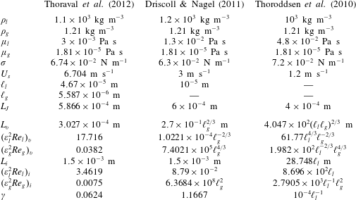
For our first example, we consider a simulation of droplet impact onto a deep pool given in Thoraval et al. (Reference Thoraval, Takehara, Etoh, Popinet, Ray, Josserand, Zaleski and Thoroddsen2012), where we have estimated
 $\ell _{l}$
,
 $\ell _{g}$
and
 $L_{J}$
from the
 $80~\unicode[STIX]{x03BC}\text{s}$
image in figure 2 in that paper. The reader should recall our comment in § 6.5 that the thin air layer here is the upper layer. Using these figures, we see from table 2 that the sensible choice is to model the air as viscous, so that
 $L$
is given by (3.4) and the reduced Reynolds number in the air is
 $\unicode[STIX]{x1D700}_{g}^{2}\mathit{Re}_{g}\sim 0.0382$
. In this regime, we find that
 $\unicode[STIX]{x1D700}_{l}^{2}\mathit{Re}_{l}\sim 17.716$
, so that the analysis for viscous air and inviscid jets in § 4.4 is most appropriate, although it is possible that this experiment falls into the regime in which the boundary layer equations hold in the jet. It should be noted that the surface-tension parameter,
 $\unicode[STIX]{x1D6FE}$
, is small in the experiments of Thoraval et al. (Reference Thoraval, Takehara, Etoh, Popinet, Ray, Josserand, Zaleski and Thoroddsen2012). This is encouraging as it suggests that we were correct to ignore surface-tension effects at leading order in the centreline equation (4.8); moreover, as discussed in appendix C, this also implies that tip retraction occurs on a longer time scale than jet growth.
Driscoll & Nagel (Reference Driscoll and Nagel2011) present a series of experiments in which a droplet spreads on a solid substrate and ejects a thin sheet from the front of the spreading lamella. Using measurements of the intensity of light emitted from an LED, the authors show that a layer of air persists between this sheet and the substrate. Here, we use the results associated with their figure 1(b). Although no estimates of the thickness of the air layer are given, the authors state that the air layer is thicker than the ejected sheet. No explicit estimate of
 $U_{s}$
is given in Driscoll & Nagel (Reference Driscoll and Nagel2011), but in Driscoll et al. (Reference Driscoll, Stevens and Nagel2010) they perform similar experiments for which the speed of the lamella at the moment when the thin sheet is ejected from the front of the lamella (cf. figure 3) is approximately
 $3~\text{m}~\text{s}^{-1}$
. Using the estimates in table 2, we see that for air layers that are much thicker than
 $\ell _{c}\sim 3.963\times 10^{-5}$
, the reduced Reynolds number in the air is large and
 $L$
is given by (3.4), which means that
 $\unicode[STIX]{x1D700}_{l}^{2}\,\mathit{Re}_{l}\ll 8.79\times 10^{-2}$
. Therefore, we would expect the analysis in the inviscid air and viscous jet regime given in § 4.2 to be the most relevant. On the other hand, for air layers much thinner than
 $\ell _{c}$
, the reduced Reynolds number in the air is small and
 $L$
is given by (3.2), so that
 $\unicode[STIX]{x1D700}_{l}^{2}\,\mathit{Re}_{l}\sim 8.79\times 10^{-2}$
. Therefore, the viscous air and viscous jet limit described in § 4.1 is the appropriate model. We note that regardless of the value of
 $\ell _{g}$
, the surface-tension parameter
 $\unicode[STIX]{x1D6FE}$
is
 $O(1)$
, which again supports our decision to neglect surface tension in the leading-order jet motion in §§ 3–4. However, in this example, surface tension will have a role in the leading-order evolution of the centreline and the retraction of the jet tip in the growing-jet model. We shall discuss this further in § 7.2.
Our third and final example concerns the spreading of a viscous droplet on a solid substrate as described in Thoroddsen et al. (Reference Thoroddsen, Takehara and Etoh2010). The authors perform several experiments and note that as the droplet spreads, air bubbles become entrained under the lamella. They show that after a certain time, the lamella detaches from the substrate and rides on a layer of air that is thinner than the lamella itself. The lower free surface of the lamella can touch down on the substrate. We take our parameter estimates from figure 2(d) in that paper, although, as shown in table 2, we do not have concrete values for either
 $\ell _{l}$
or
 $\ell _{g}$
in this example. However, given that the air layer is suggested to be much thinner than the lamella, we postulate that the viscous air regime might be most appropriate, and can therefore compare
 $L$
calculated using (3.2) with
 $L_{J}$
and check the size of the resulting reduced Reynolds number in the air. For the air to be viscous, we require
 $$\begin{eqnarray}L_{J}>L\approx (4.05\times 10^{2})(\ell _{l}\ell _{g})^{2/3}~\text{m}\end{eqnarray}$$
and
 $$\begin{eqnarray}1\gg \unicode[STIX]{x1D700}_{g}^{2}\,\mathit{Re}_{g}=(1.982\times 10^{2})\frac{\ell _{g}^{4/3}}{\ell _{l}^{2/3}}.\end{eqnarray}$$
If the lamella had thickness
 $\ell _{l}\sim 10^{-4}$
m, an air layer thickness of
 $\ell _{g}\sim 10^{-5}$
m would satisfy (7.1) and (7.2), which does not seem to be implausible. In such an example, the reduced Reynolds number in the jet would also be small, so that the model in § 4.1 would be the most appropriate regime.
Although it would be desirable to have more data to compare with, there is good evidence that the length scales given by (3.2) and (3.4) are suitable for a range of scenarios, and, in addition, each of the regimes presented in §§ 4.1–4.4 may be relevant in different splashing/impact problems.
7.2 Summary
In this paper, we have presented models that investigate the role of an air-cushioning layer on the evolution of a liquid jet. Inspired by the splash jets produced in impact problems, as depicted in figures 2–3, we considered a long thin jet of liquid moving over a solid substrate with a thin layer of air cushioning it from the solid. Above the jet is a larger unbounded air region. In each model, we considered the limit in which deflections to the jet centreline are driven by the jump in air pressure across the jet. We looked at various regimes depending on the size of the reduced Reynolds number in each phase. The appropriate horizontal length scale of such deflections is given by
 $$\begin{eqnarray}L=L_{v}=\left(\frac{\unicode[STIX]{x1D70C}_{l}U_{s}\ell _{l}^{2}\ell _{g}^{2}}{\unicode[STIX]{x1D707}_{g}}\right)^{1/3}\end{eqnarray}$$
when the reduced Reynolds number in the air is small, so that viscous forces dominate, and by
 $$\begin{eqnarray}L=L_{i}=\frac{\ell _{l}\unicode[STIX]{x1D70C}_{l}^{1/2}}{\unicode[STIX]{x1D70C}_{g}^{1/2}}\end{eqnarray}$$
when the reduced Reynolds number is large, so that inertial forces dominate.
We considered the stability to small perturbations of an infinitely long constant-speed, constant-thickness liquid jet travelling over a constant-thickness air layer. We showed that the centreline of such a jet is destabilised by the pressure jump across it provided that the surface tension is sufficiently small. This is true both when the air is viscous dominated and when it is inertia dominated, and in each case we derived the wavenumber of the fastest-growing mode, given by (5.11) and (5.12) for the viscous air case and by (5.18) for the inviscid case. While comparisons were purely qualitative, we demonstrated that the experiments in Thoraval et al. (Reference Thoraval, Takehara, Etoh and Thoroddsen2013) fell into the viscous gas regime, so that ejecta instability could potentially be a mechanism for air bubble entrapment.
In § 6, we moved on to consider a jet emitted from a nozzle, concentrating on the regime in which the reduced Reynolds number in the air layer is small, so that the jet length scale is given by (7.3). We considered a constant-speed, constant-thickness jet shooting from a fixed orifice over a thin air cushion. After discussing the relevant scalings in the tip region in appendix C, we considered the particular regime in which retraction of the jet tip due to the action of surface tension happens on a longer time scale than the jet growth. By making a change of variables, we showed how the resulting equations can be related to the motion of a string on top of a thin air layer, and used this to motivate the boundary and initial conditions required to close the problem. When the surface tension is small, we only require one boundary condition at the jet tip: we imposed atmospheric air pressure motivated by the scaling arguments in appendix C. At the nozzle, we imposed boundary conditions fixing the thickness of the air cushion and the angle at which the jet is fired, while allowing no flux of air under the nozzle. By solving the resulting problem numerically, we were able to show that the jet bends as it advances due to the action of the air layer. Furthermore, we gave evidence that the jet can eventually touch the solid substrate away from its tip, which is reminiscent of the onset of droplet sling-shotting seen in droplet impact experiments in Thoraval et al. (Reference Thoraval, Takehara, Etoh, Popinet, Ray, Josserand, Zaleski and Thoroddsen2012); cf. figure 2 (note that, in this figure, the thin layer is between the jet and the main droplet).
Both of these models indicate the regimes in which the jet motion may be heavily influenced by the surrounding air as it grows, and thus it cannot be ignored in any modelling or study of splash jets. In particular, the simultaneous small aspect ratios of the jet and the air layer, as well as the relevance of the substrate in the tip region, are key in the evolution of the jet centreline, and these have often been neglected in existing models. Furthermore, the growing-jet model we considered in § 6 showed qualitatively similar behaviour to splash jets seen in droplet impacts. However, any in-depth comparisons require several further details.
In terms of theory, there are plenty of future areas of interest. There are several simple extensions to cover other scenarios: for example, replacing the solid substrate with a deep liquid pool, which is more relevant in the experiments of Thoraval et al. (Reference Thoraval, Takehara, Etoh, Popinet, Ray, Josserand, Zaleski and Thoroddsen2012) and Agbaglah et al. (Reference Agbaglah, Thoraval, Thoroddsen, Zhang, Fezzaa and Deegan2015); considering limits in which the jet is much thinner than the cushioning layer or vice versa; or considering asymptotic regimes in which the reduced Reynolds numbers in either phase are of order unity.
The touchdown process should also be investigated in more detail. While our zero-surface-tension model predicts a finite-time touchdown, it is well known (see, e.g., Duchemin & Josserand Reference Duchemin and Josserand2011) that surface tension inhibits touchdown in related problems, so a more careful analysis is necessary. Furthermore, for sufficiently thin air layers, it is likely that non-continuum effects will play a role in the evolution through the Knudsen number. Such an analysis is beyond the scope of this paper, but non-continuum effects can be incorporated via an effective slip at the solid–gas and liquid–gas interfaces; see Marchand et al. (Reference Marchand, Chan, Snoeijer and Andreotti2012), Riboux & Gordillo (Reference Riboux and Gordillo2014) and Sprittles (Reference Sprittles2017). This perturbation to the boundary condition alters the local lubrication model in the air layer, which in turn will influence the centreline evolution.
Major areas for future work concern the growing jet: namely the small-time jet growth, the flow around the jet tip and the boundary conditions at the jet root. We shall now discuss these in slightly more detail.
In this paper, we have primarily focused on jets and lamellae that have attained the characteristic small aspect ratio seen in experiments and depicted in figures 2–3. It is therefore important to check whether the earlier dynamics, when the nascent jet or lamella has an order-unity aspect ratio, plays a significant role in the long-time evolution. It is particularly interesting in light of recent experiments by Zhang et al. (Reference Zhang, Toole, Fezzaa and Deegan2012a ,Reference Zhang, Toole, Fezzaa and Deegan b ) and Agbaglah et al. (Reference Agbaglah, Thoraval, Thoroddsen, Zhang, Fezzaa and Deegan2015) that multiple jets can form when a droplet impacts a deep pool. These jets may coalesce with one another, the droplet or the later-emerging lamella, but all are examples of liquid jets moving over a narrow air gap. Moreover, in this early stage of impact, vorticity shedding at the jet root may also be important, as discussed in Thoraval et al. (Reference Thoraval, Takehara, Etoh, Popinet, Ray, Josserand, Zaleski and Thoroddsen2012), Moore et al. (Reference Moore, Ockendon, Ockendon and Oliver2014) and Agbaglah et al. (Reference Agbaglah, Thoraval, Thoroddsen, Zhang, Fezzaa and Deegan2015).
The flow around the jet tip is perhaps the most important outstanding question. Our assumption in this paper has been that the amount of fluid in the jet tip is small compared with that in the bulk of the jet, and that the flow around the tip is well represented by applying an air pressure condition there. However, as discussed in appendix C, for sufficiently large surface tension, tip retraction occurs at leading order in the growing-jet problem considered in § 6, which makes the problem more complicated. In the outer region discussed in § 6.1, the approximation that the jet tip moves ballistically with the initial jet speed is no longer appropriate: the jet loses mass and momentum to the tip, so the tip location needs to be determined as part of the problem. Introduction of surface tension to (6.2) in the
 $(\unicode[STIX]{x1D709},t)$
frame gives
 $$\begin{eqnarray}H_{t}+\left(-\frac{H}{2}-\frac{1}{12}H^{3}P_{\unicode[STIX]{x1D709}}\right)_{\unicode[STIX]{x1D709}}=0,\quad -\unicode[STIX]{x1D6FE}H_{\unicode[STIX]{x1D709}\unicode[STIX]{x1D709}}+H_{tt}=P.\end{eqnarray}$$
To tackle (7.5), we would need to determine whether we need a further boundary condition at the tip. This depends on the speed of tip retraction (see Moore Reference Moore2014), and would involve coupling to an in-depth tip-flow model.
It is possible that some of the ideas from the related field of sheet retraction could be employed in modelling of the tip in such cases; see, for example, Erneux & Davis (Reference Erneux and Davis1993), Savva & Bush (Reference Savva and Bush2009), Gordillo et al. (Reference Gordillo, Agbaglah, Duchemin and Josserand2011) and the references therein. When a thin liquid sheet is punctured, it can either retract or work to close up the resulting hole. Typical models derive a thin-film approximation in the main part of the sheet, similar to our models in § 4. However, despite the lack of asymptotic robustness, use of the same thin-film approximation in the rim is shown to give surprisingly accurate results to full numerical simulations; see, for example, Gordillo et al. (Reference Gordillo, Agbaglah, Duchemin and Josserand2011). A similar ad hoc approach may bear fruit in our growing-jet model. Similarly, vertical and horizontal force balances akin to those in Riboux & Gordillo (Reference Riboux and Gordillo2015) could also be used as approximations to the tip dynamics, although the role of the solid substrate must be taken into account when the tip is sufficiently close to the substrate.
At the jet root, it is probable that we need to think more closely about the flow in both the liquid and the air. A possible approach would be to match the jet to a Wagner-type inner region, as discussed in Howison et al. (Reference Howison, Ockendon and Wilson1991) or Moore et al. (Reference Moore, Ockendon and Oliver2013) with surrounding air. It is also possible to account for the role of viscous forces in the jet-root region; see, for example, Riboux & Gordillo (Reference Riboux and Gordillo2015). Moreover, as mentioned previously, there is strong evidence that vorticity accumulates and can shed from the base of splash jets, so it is likely that this needs to be taken into account in any modelling.
At a more basic level, all of our analysis in this paper has been restricted to two dimensions, whereas three-dimensional effects may be important in describing some of the phenomena seen in the aforementioned experiments. Fortunately, it is relatively straightforward to extend our jet models to three dimensions, as reported in Moore (Reference Moore2014).
In this paper, we have presented several possible models to describe the evolution of liquid jets in the presence of a thin cushioning air layer. We have identified the governing physics of the problem, deriving the crucial length scales involved for different regimes. Moreover, we have shown that the resulting models are unstable to small perturbations of the jet centreline and the air pressure, and that it is possible to make the jet centreline bend purely due to the action of an air pressure jump. This indicates that the presence of a thin layer of air can be a mechanism for the bending and touchdown of splash jets, or the instability of a lamella that has become detached from a substrate. The models here are intended to be useful tools for future studies of impact problems. The equations of motion can be coupled with more sophisticated models of the flow behaviour near the jet root and jet tip (such as those in Riboux & Gordillo Reference Riboux and Gordillo2015), or adapted for different geometries. The key results are the systematic derivation of reduced models governing the evolution of the jet centreline when it is deflected by an air-cushioning layer and the fact that the resulting motion leads to potential new mechanisms for jet touchdown and air entrapment.
Acknowledgements
The authors would like to thank M.-J. Thoraval, S. T. Thoroddsen, A. A. Korobkin and S. J. Chapman for helpful comments in the course of this work. M.R.M. is grateful to the EPSRC for a studentship that he received while working on part of this study. This publication was based on work supported in part by award no. KUK-C1-013-04, made by King Abdullah University of Science and Technology (KAUST). The authors are grateful to the anonymous referees whose comments improved this paper significantly.
Appendix A. Stronger surface tension
Thus far we have taken surface-tension effects to be small, specifically,
 $\mathit{We}=O(1/\unicode[STIX]{x1D700}_{l})$
. However, taking inspiration from Howell (Reference Howell1996), it is worth noting how the model changes for smaller values of the Weber number. We shall concentrate on the viscous air and viscous jet case described in § 4.1, but the ideas extend readily. We define a new surface-tension parameter,
 $$\begin{eqnarray}\bar{\unicode[STIX]{x1D6FE}}=\frac{2\unicode[STIX]{x1D700}_{l}}{\mathit{We}}=O(1),\end{eqnarray}$$
so that surface tension enters the leading-order dynamic boundary conditions. In order to retain the air pressure in the leading-order model, we find that
 $L$
is slightly different from the deflection length scale for viscous air (3.2), since we must balance the air pressure with the large-surface-tension term in the normal stress condition on the lower free surface (2.15). Thus, we require that
 $\unicode[STIX]{x1D706}=O(1/\unicode[STIX]{x1D700}_{l}^{2})$
, and therefore
 $$\begin{eqnarray}L=\frac{\unicode[STIX]{x1D70C}_{l}\ell _{g}^{2}U_{s}}{\unicode[STIX]{x1D707}_{g}}\end{eqnarray}$$
is the appropriate deflection length scale in this large-surface-tension regime. In general, this is longer than the length scales given in (3.2) and (3.4).
With these assumptions, and proceeding as in § 4.1, to leading order, conservation of mass in the jet gives (4.1). However, since we require the leading-order jet pressure to be constant across the jet, the dynamic boundary conditions (2.14) and (2.15) imply that
 $$\begin{eqnarray}\bar{\unicode[STIX]{x1D6FE}}\left(\unicode[STIX]{x1D702}H_{xx}+\frac{h_{xx}}{2}\right)+P=0,\end{eqnarray}$$
where the leading-order air pressure satisfies the lubrication equation (4.2). Without the air pressure term, (A 3) simply states that the curvature of the centreline does not vary to leading order; cf. Howell (Reference Howell1994). Thus, the leading-order jet pressure is given by
 $$\begin{eqnarray}p=-\frac{2}{\mathit{Re}_{l}}u_{x}+P+\frac{\bar{\unicode[STIX]{x1D6FE}}\unicode[STIX]{x1D702}}{2}H_{xx},\end{eqnarray}$$
so that, proceeding to
 $O(\unicode[STIX]{x1D700}_{l}^{2})$
in the analysis, we derive the extensional flow equation
 $$\begin{eqnarray}h(u_{t}+uu_{x})=\frac{4}{\mathit{Re}_{l}}(hu_{x})_{x}+\frac{\bar{\unicode[STIX]{x1D6FE}}}{4}hh_{xxx}-\frac{hP_{x}}{2}.\end{eqnarray}$$
Therefore, for larger surface tension, the jet and air motions are coupled and governed by (4.1), (4.2), (A 3) and (A 5). It should be noted that we can use (A 3) to eliminate
 $H$
from (4.2) and solve for
 $u$
,
 $h$
and
 $P$
from (4.1) and (4.2) combined with (A 5). We shall not attempt to solve this coupled system in this paper.
Appendix B. Derivation of the pressure-jump equation
We present here a derivation of the centreline deflection equation in the viscous air and viscous liquid regime (4.4). To leading order, we know that
 $$\begin{eqnarray}u=u(x,t),\quad v=-u_{x}\bar{y}+\unicode[STIX]{x1D702}(H_{t}+(uH)_{x}).\end{eqnarray}$$
Thus, utilising the extensional flow equation (4.3), the
 $O(\unicode[STIX]{x1D700}_{l}^{2})$
correction to the tangential jet velocity,
 $u^{(1)}$
, must satisfy
 $$\begin{eqnarray}u_{\bar{y}\bar{y}}^{(1)}=\frac{4}{h}(hu_{x})_{x}-3u_{xx},\end{eqnarray}$$
subject to the shear stress conditions
 $$\begin{eqnarray}\displaystyle & u_{\bar{y}}^{(1)}=4(\unicode[STIX]{x1D702}H_{x}+h_{x})-v_{x}\quad \text{on}~\bar{y}=\unicode[STIX]{x1D702}H+h, & \displaystyle\end{eqnarray}$$
 $$\begin{eqnarray}\displaystyle & u_{\bar{y}}^{(1)}=4\unicode[STIX]{x1D702}H_{x}-v_{x}\quad \text{on}~\bar{y}=\unicode[STIX]{x1D702}H, & \displaystyle\end{eqnarray}$$
giving
 $$\begin{eqnarray}[u_{\bar{y}}^{(1)}]_{\bar{y}=\unicode[STIX]{x1D702}H}^{\bar{y}=\unicode[STIX]{x1D702}H+h}=4h_{x}u_{x}+hu_{xx}\end{eqnarray}$$
and
 $$\begin{eqnarray}\displaystyle [u_{x}^{(1)}]_{\bar{y}=\unicode[STIX]{x1D702}H}^{\bar{y}=\unicode[STIX]{x1D702}H+h} & = & \displaystyle \left(\frac{4h_{x}u_{x}}{h}+u_{xx}\right)_{x}\frac{h^{2}}{2}-\unicode[STIX]{x1D702}H_{x}h\left(\frac{4h_{x}u_{x}}{h}+u_{xx}\right)\nonumber\\ \displaystyle & & \displaystyle +\,h(4\unicode[STIX]{x1D702}H_{x}u_{x}+\unicode[STIX]{x1D702}Hu_{xx}-\unicode[STIX]{x1D702}(H_{tx}+(uH)_{xx}))_{x}.\end{eqnarray}$$
At
 $O(\unicode[STIX]{x1D700}_{l}^{2})$
, the normal stress conditions (2.14) and (2.15) give
 $$\begin{eqnarray}p=-\frac{\unicode[STIX]{x1D6FE}}{2}(\unicode[STIX]{x1D702}H_{xx}+h_{xx})+\frac{2}{\mathit{Re}_{l}}[2(\unicode[STIX]{x1D702}H_{x}+h_{x})^{2}u_{x}-u_{x}^{(1)}-(\unicode[STIX]{x1D702}H_{x}+h_{x})(u_{\bar{y}}^{(1)}+v_{x})]\end{eqnarray}$$
on
 $\bar{y}=\unicode[STIX]{x1D702}H+h$
and
 $$\begin{eqnarray}p=\unicode[STIX]{x1D706}P+\frac{\unicode[STIX]{x1D6FE}}{2}\unicode[STIX]{x1D702}H_{xx}+\frac{2}{\mathit{Re}_{l}}[2\unicode[STIX]{x1D702}^{2}H_{x}^{2}u_{x}-u_{x}^{(1)}-\unicode[STIX]{x1D702}H_{x}(u_{\bar{y}}^{(1)}+v_{x})]\end{eqnarray}$$
on
 $\bar{y}=\unicode[STIX]{x1D702}H$
.
Now, at second order, the vertical component of the Navier–Stokes momentum equation (2.2) is given by
 $$\begin{eqnarray}\mathit{Re}_{l}(v_{t}+uv_{x}+vv_{\bar{y}})=-\mathit{Re}_{l}\,p_{\bar{y}}^{(1)}+v_{xx}+v_{\bar{y}\bar{y}}^{(1)}-\mathit{Re}_{l}\,{\mathcal{F}}.\end{eqnarray}$$
Upon integrating across the layer, the left-hand side of (B 9) becomes
 $$\begin{eqnarray}\mathit{Re}_{l}[\bar{v}_{t}+u\bar{v}_{x}-\bar{v}u_{x}-(\unicode[STIX]{x1D702}(H_{t}+uH_{x})+h_{t}+uh_{x})^{2}+\unicode[STIX]{x1D702}^{2}(H_{t}+uH_{x})^{2}],\end{eqnarray}$$
where
 $$\begin{eqnarray}\bar{v}=\int _{\unicode[STIX]{x1D702}H}^{\unicode[STIX]{x1D702}H+h}v\,\text{d}\bar{y}=h\left(-\frac{hu_{x}}{2}+\unicode[STIX]{x1D702}(H_{t}+uH_{x})\right).\end{eqnarray}$$
Thus, the left-hand side of (B 9) becomes
 $$\begin{eqnarray}\mathit{Re}_{l}\left[h^{2}u_{x}^{2}+\unicode[STIX]{x1D702}h(u^{2}H_{xx}+2uH_{xt}+H_{tt})-\frac{h^{2}}{2}\left(\frac{4(hu_{x})_{x}}{h}\right)_{x}+4\unicode[STIX]{x1D702}H_{x}(hu_{x})_{x}\right].\end{eqnarray}$$
Similarly, utilising (B 5)–(B 8), the right-hand side of (B 9) is given by
 $$\begin{eqnarray}\unicode[STIX]{x1D706}\,\mathit{Re}_{l}\,P+\unicode[STIX]{x1D6FE}\,\mathit{Re}_{l}\left(\unicode[STIX]{x1D702}H_{xx}+\frac{h_{xx}}{2}\right)-\mathit{Re}_{l}\,{\mathcal{F}}h+2(hh_{x}u_{x})_{x}+4\unicode[STIX]{x1D702}(hH_{x}u_{x})_{x}.\end{eqnarray}$$
Appendix C. Tip region for a growing jet
At the end of the jet, the free surface of the liquid turns over, forming a tip surrounded by air, in an inner region of size of
 $O(\unicode[STIX]{x1D700}_{l})$
, at least for times of order unity, as depicted in figure 12. The key difference from Riboux & Gordillo (Reference Riboux and Gordillo2014, Reference Riboux and Gordillo2015) is the presence of the solid base, which must be important in the tip motion when the air gap thickness is comparable to the size of the tip. For ease of matching back to the outer region, we shall continue to use
 $H^{\ast }$
and
 $h^{\ast }$
to denote the lower air layer thickness and jet thickness respectively. Clearly,
 $h^{\ast }$
vanishes at the tip itself.
Local to the jet tip, the free surface becomes rounded due to the action of surface tension and/or the air, meaning that the tip location as predicted by the outer region (i.e. the region discussed in § 6) in the absence of surface tension,
 $x^{\ast }=U_{s}t^{\ast }$
, is not applicable. We consider a region with order-unity aspect ratio about
 $x^{\ast }=U_{s}t^{\ast }$
to investigate tip retraction.

In this appendix, we shall concentrate on the regime in which the reduced Reynolds number in the outer air region is small, so that the Reynolds lubrication equation (4.2) holds in the lower air layer of the ‘outer’ region described in § 6. This means that upstream in the lower air layer in the tip region, there is an
 $O(U_{s})$
variation in the air speed from the no-slip condition on the substrate to the continuity of velocity condition on the lower free surface. We also continue to assume that
 $\unicode[STIX]{x1D702}=O(1)$
, and we stress that the tip region for cases where
 $\unicode[STIX]{x1D702}\rightarrow 0$
or
 $\unicode[STIX]{x1D702}\rightarrow \infty$
will be markedly different.
Assuming for the time being that the tip does not retract back into the jet and that it is of size
 $O(1)$
, we consider a frame that moves with the location of the jet tip in the absence of surface tension by setting
 $$\begin{eqnarray}x^{\ast }=U_{s}t^{\ast }+\ell _{l}\tilde{x},\quad y^{\ast }=\ell _{l}{\tilde{y}},\quad t^{\ast }=\frac{L}{U_{s}}t.\end{eqnarray}$$
The air layer thickness and jet thickness scale, as before, with
 $$\begin{eqnarray}H^{\ast }=\ell _{g}\tilde{H},\quad h^{\ast }=\ell _{l}\tilde{h}.\end{eqnarray}$$
As discussed above, the velocity scales in the air are given by
 $$\begin{eqnarray}U^{\ast }=U_{s}\tilde{U} ,\quad V^{\ast }=U_{s}\tilde{V},\quad P^{\ast }={\mathcal{P}}_{t}\tilde{P},\end{eqnarray}$$
while the appropriate pressure scale
 ${\mathcal{P}}_{t}$
is chosen to maintain a leading-order balance in the horizontal momentum Navier–Stokes equation (2.4): when
 $\unicode[STIX]{x1D700}_{g}Re_{g}=O(1)$
, we must set
 ${\mathcal{P}}_{t}=\unicode[STIX]{x1D707}_{g}U_{s}/\ell _{l}$
, while when
 $\unicode[STIX]{x1D700}_{g}Re_{g}\gg 1$
, we must set
 ${\mathcal{P}}_{t}=\unicode[STIX]{x1D70C}_{g}U_{s}^{2}$
.
The jet pressure is taken to balance the term due to surface tension in the normal stress boundary condition (2.14), so we take
 $$\begin{eqnarray}p^{\ast }=\frac{\unicode[STIX]{x1D70E}}{\ell _{l}}\tilde{p}.\end{eqnarray}$$
It should be noted that for very small
 $\unicode[STIX]{x1D70E}$
(equivalent to
 $\unicode[STIX]{x1D6FE}\ll \unicode[STIX]{x1D700}_{l}^{3}$
), this scaling is invalid since the surface tension is so small that the jet motion in the tip region is driven by the air. We shall ignore this possibility here, since this involves values of
 $\unicode[STIX]{x1D6FE}$
that are not realistic for the various experiments we consider in § 7.1.
The appropriate scaling for the jet velocity is determined from the horizontal momentum Navier–Stokes equation (2.1) and depends on the size of
 $\unicode[STIX]{x1D6FE}$
and the pressure scale
 ${\mathcal{P}}_{t}$
. We shall discuss the case in which
 ${\mathcal{P}}_{t}=\unicode[STIX]{x1D707}_{g}U_{s}/\ell _{l}$
in detail here, but the analysis is readily extended to cases in which we choose the inertial scale. For
 $\unicode[STIX]{x1D700}_{l}^{3}\leqslant \unicode[STIX]{x1D6FE}\leqslant \unicode[STIX]{x1D700}_{l}^{2}$
, we take the velocity scale to be
 $\unicode[STIX]{x1D6FE}U_{s}/(2\unicode[STIX]{x1D700}_{l})$
. Clearly, this is much less than
 $U_{s}$
, so that the retraction of the tip is small on the jet growth time scale. For
 $\unicode[STIX]{x1D700}_{l}^{2}\leqslant \unicode[STIX]{x1D6FE}\leqslant 1$
, we take the Taylor–Culick scale
 $\sqrt{\unicode[STIX]{x1D6FE}/2}U_{s}$
. Hence, the liquid velocity scale is smaller than the air velocity scale when
 $\unicode[STIX]{x1D6FE}=o(1)$
.
Thus, we only see leading-order retraction when
 $\unicode[STIX]{x1D6FE}=O(1)$
, while, for
 $\unicode[STIX]{x1D6FE}\ll 1$
, we can effectively ignore the retraction of the tip due to the effects of surface tension and air flow around the tip. In the outer region, this means that
 $x=t$
is the correct leading-order approximation for the tip location when
 $\unicode[STIX]{x1D6FE}\ll 1$
. Moreover, since the pressure scale is an order of magnitude smaller than the outer pressure scale (3.1), the appropriate matching condition for the leading-order air pressure in the outer region is given by (6.3d
), as discussed in § 6.1.
Appendix D. Numerical methods
In this appendix, we outline the two numerical schemes that we used to compute solutions of (6.1) subject to (6.3).
D.1 Implicit Euler solver
Making the coordinate transformation
 $\unicode[STIX]{x1D709}=x-t$
, we seek to solve
 $$\begin{eqnarray}V-\frac{H_{\unicode[STIX]{x1D709}}}{2}=Q_{\unicode[STIX]{x1D709}},\quad V_{t}=P,\quad V=H_{t},\quad Q=\frac{H^{3}P_{\unicode[STIX]{x1D709}}}{12}\end{eqnarray}$$
on
 $-t<\unicode[STIX]{x1D709}<0$
,
 $t>0$
subject to
 $$\begin{eqnarray}H(-t,t)=H_{J}(t),\quad V(-t,t)={\dot{H}}_{J}(t)+G_{J}(t),\quad Q(-t,t)=\frac{H_{J}(t)}{2},\quad P(0,t)=0,\end{eqnarray}$$
where we have introduced the dependent variables
 $V$
and
 $Q$
so that all of the derivatives are first order in (D 1). We fix an initial time station,
 $t=t_{0}$
, and discretise the spatial domain as follows:
 $-t_{0}=\unicode[STIX]{x1D709}_{1}<\unicode[STIX]{x1D709}_{2}<\cdots <\unicode[STIX]{x1D709}_{M}=0$
, where the uniform spacing is given by
 $\unicode[STIX]{x0394}\unicode[STIX]{x1D709}$
. We use (6.4) and (6.5) to calculate our initial solution on this grid.
At time
 $t=t_{1}=t_{0}+\unicode[STIX]{x0394}\unicode[STIX]{x1D709}$
, we introduce the new point
 $\unicode[STIX]{x1D709}_{0}=-t_{1}$
, at which we know
 $H$
,
 $V$
and
 $Q$
from the boundary data (D 2). We also know
 $P=0$
at
 $\unicode[STIX]{x1D709}=0$
. We discretise (D 1) using an implicit Euler scheme and solve the resulting nonlinear system using Newton’s method (see, for example, Süli & Mayers Reference Süli and Mayers2003) until we achieve the required tolerance. The procedure is repeated at each time step.
A log–log plot showing the convergence of
 $H$
and
 $P$
as we decrease
 $\unicode[STIX]{x0394}\unicode[STIX]{x1D709}$
, to the solution
 $H_{0.0001}$
,
 $P_{0.0001}$
for
 $\unicode[STIX]{x0394}\unicode[STIX]{x1D709}=0.0001$
at a fixed time before touchdown.

In figure 13, we compare the numerical results for the jet height and air pressure at a fixed time before touchdown for a range of values of
 $\unicode[STIX]{x0394}\unicode[STIX]{x1D709}$
against the solution on a very fine grid, where
 $\unicode[STIX]{x0394}\unicode[STIX]{x1D709}=10^{-4}$
. We have again chosen
 $H_{J}(t)=1$
and
 $G_{J}(t)=0$
. Specifically, we take
 $\unicode[STIX]{x0394}\unicode[STIX]{x1D709}=0.01$
, 0.005, 0.002, 0.001 and 0.0005. The solution converges as we decrease the spatial step size, although the pressure solution converges more slowly. This is as a result of the large pressure peaks that form underneath the minima on the jet, as can be seen in figure 8(c). Nonetheless, we have good evidence that the code is producing the correct solution. In addition, there is good comparison with the small-time solution (6.4), (6.5), as we see in figure 8(a).
D.2 Finite element solution of (6.1) and (6.3)
We calculate a numerical solution of (6.1) and (6.3) by first transforming to the fixed domain
 $0<X<1$
using the change of variable
 $X=x/t$
. The differential equations (6.1) then become
 $$\begin{eqnarray}\displaystyle & \displaystyle H_{t}-\frac{2X-1}{2t}H_{X}=\left(\frac{H^{3}}{12t^{2}}P_{X}\right)_{X}, & \displaystyle\end{eqnarray}$$
 $$\begin{eqnarray}\displaystyle & \displaystyle H_{tt}-\frac{2(X-1)}{t}H_{Xt}+\frac{(X-1)^{2}}{t^{2}}H_{XX}+\frac{2(X-1)}{t^{2}}H_{X}=P & \displaystyle\end{eqnarray}$$
and the boundary conditions (6.3) become
 $$\begin{eqnarray}\displaystyle & H(0,t)=H_{J}(t), & \displaystyle\end{eqnarray}$$
 $$\begin{eqnarray}\displaystyle & H_{X}(0,t)=tG_{J}(t), & \displaystyle\end{eqnarray}$$
 $$\begin{eqnarray}\displaystyle & \displaystyle P_{X}(0,t)=\frac{6t}{(H_{J}(t))^{2}}, & \displaystyle\end{eqnarray}$$
 $$\begin{eqnarray}\displaystyle & P(1,t)=0. & \displaystyle\end{eqnarray}$$
We may solve (D 3) as an equation for
 $P$
, with boundary conditions given by (D 7) and (D 8). By introducing a new variable
 $q(X,t)$
, we may decompose (D 4) into the system of first-order hyperbolic equations
 $$\begin{eqnarray}\displaystyle & \displaystyle H_{t}+\left(\frac{1-X}{t}H\right)_{X}=q, & \displaystyle\end{eqnarray}$$
 $$\begin{eqnarray}\displaystyle & \displaystyle q_{t}+\left(\frac{1-X}{t}q\right)_{X}=P-\frac{2q}{t}. & \displaystyle\end{eqnarray}$$
The only inflow boundary conditions for (D 9) and (D 10) are at
 $X=0$
. The boundary condition given by (D 5) may be used as a boundary condition for (D 9) at
 $X=0$
. By using (D 5), (D 6) and (D 9), we may deduce a boundary condition for (D 10) at
 $X=0$
, given by
 $$\begin{eqnarray}q(0,t)=\frac{\text{d}H_{J}}{\text{d}t}-\frac{H_{J}(t)}{t}+G_{J}(t).\end{eqnarray}$$
A numerical solution of the system of equations discussed above was calculated using the continuous Galerkin finite element method; see, for example, Eriksson et al. (Reference Eriksson, Estep, Hansbo and Johnson1996). The domain
 $0<X<1$
was discretised into
 $N$
elements, and a constant time step
 $\unicode[STIX]{x0394}t$
was used to progress the solution in time. A linear approximation was made to
 $H$
,
 $P$
and
 $q$
on each element, and an implicit approximation was made to all time derivatives. The discretised system of nonlinear algebraic equations arising from this discretisation on each time step was solved using Newton’s method. Both the element length and the time step were reduced until the solution was sufficiently accurate, and results were compared with both the small-time solution (6.4), (6.5) and the implicit Euler solver described in § D.1 to check validity, as discussed in Moore (Reference Moore2014).