1 Introduction
Droplet shape deformations have been extensively studied in many different contexts, both at the fundamental level and also for specific applications with industrial and biomedical relevance that require a good understanding of how droplets deform. Starting from the pioneering work of Taylor (Reference Taylor1934), deformation of fluid drops by shear flows of Newtonian (Cox Reference Cox1969; Schmitz & Felderhof Reference Schmitz and Felderhof1982; Rallison Reference Rallison1984; Tretheway & Leal Reference Tretheway and Leal2001) and complex (Chilcott & Rallison Reference Chilcott and Rallison1988; Ramaswamy & Leal Reference Ramaswamy and Leal1999; Zhou et al. Reference Zhou, Yue, Feng, Ollivier-Gooch and Hu2010) fluids has been extensively studied. These studies have important implications for several problems, such as emulsion flows as well as many industrial applications, including food processing, pharmaceutical manufacturing, etc. (Nielloud & Marti-Mestres Reference Nielloud and Marti-Mestres2000; Friberg, Larsson & Sjoblom Reference Friberg, Larsson and Sjoblom2003; Sjoblom Reference Sjoblom2005). In addition to the studies of droplet deformation and dynamics in shear flows, various works have focused on drop deformations generated by body forces, including drops deformed under the action of electric (Allan & Mason Reference Allan and Mason1962; Taylor Reference Taylor1964; Rosenkilde Reference Rosenkilde1969; Miksis Reference Miksis1981; Wohlhuter & Basaran Reference Wohlhuter and Basaran1992) and magnetic (Bacri & Salin Reference Bacri and Salin1982; Sero-Guillaume et al. Reference Sero-Guillaume, Zouaoui, Bernardin and Brancher1992) fields.
The theoretical study of drop deformation under an applied electric field for nearly spherical drops (Allan & Mason Reference Allan and Mason1962) provided important insights into the subject. Equilibrium deformation and stability of conducting (Taylor Reference Taylor1964) and linear dielectric (Rosenkilde Reference Rosenkilde1969) drops under an electric field were then studied assuming ellipsoidal drop shapes for small to moderate deformations. Relaxing the ellipsoidal shapes assumption, the axisymmetric shapes and stability of linear (Miksis Reference Miksis1981; Wohlhuter & Basaran Reference Wohlhuter and Basaran1992) and nonlinear (Basaran & Wohlhuter Reference Basaran and Wohlhuter1992; Wohlhuter & Basaran Reference Wohlhuter and Basaran1993) dielectric drops were studied numerically. All these works reported bistable drop shapes (Bacri & Salin Reference Bacri and Salin1982) above a certain threshold of relative permittivity of drops to the surrounding media.
Described by equations mathematically equivalent to those governing uncharged dielectric drops, the deformations of ferrofluid drops (Rosensweig Reference Rosensweig2013) under the effect of magnetic fields have also been independently studied. Deformation of linear ferrofluid drops was studied for small (Arkhipenko, Barkov & Bashtovoi Reference Arkhipenko, Barkov and Bashtovoi1979; Tsebers Reference Tsebers1985) and finite (Afkhami et al. Reference Afkhami, Tyler, Renardy, Renardy, St Pierre, Woodward and Riffle2010) deformations by assuming ellipsoidal shapes. The exact equilibrium shapes of linear ferrofluid drops under the action of a magnetic field were then obtained numerically, and large mean curvature at the tips compared to that of ellipsoids was reported (Sero-Guillaume et al. Reference Sero-Guillaume, Zouaoui, Bernardin and Brancher1992). The exact equilibrium shapes of linear ferrofluid on a solid surface were also studied experimentally (Zhu et al. Reference Zhu, Nguyen, Ramanujan and Huang2011). The bistability of equilibrium drop shapes above a certain ferrofluid susceptibility, which was first observed by Bacri & Salin (Reference Bacri and Salin1982) for ferrofluid drops, was later observed also for dielectric drops. This observed bistability in ferrofluid drop equilibrium shapes was studied numerically for linear ferrofluid drops (Lavrova et al. Reference Lavrova, Matthies, Polevikov and Tobiska2004, Reference Lavrova, Matthies, Mitkova, Polevikov and Tobiska2006).
The dynamics and stability of dielectric and magnetic fluids have been studied under diverse conditions. Destabilization of the interface between a ferrofluid and a non-magnetic fluid was discussed first by Boudouvis et al. (Reference Boudouvis, Puchalla, Scriven and Rosensweig1987), and explored further by Engel, Langer & Chetverikov (Reference Engel, Langer and Chetverikov1999), Abou, Wesfreid & Roux (Reference Abou, Wesfreid and Roux2000), Lavrova et al. (Reference Lavrova, Matthies, Mitkova, Polevikov and Tobiska2006), Gollwitzer et al. (Reference Gollwitzer, Matthies, Richter, Rehberg and Tobiska2007), Chen & Cheng (Reference Chen and Cheng2008), Mizuta (Reference Mizuta2011) and Cao & Ding (Reference Cao and Ding2014). Multiple works studied the breakup of drops under electric (Sherwood Reference Sherwood1988; Basaran et al. Reference Basaran, Patzek, Benner and Scriven1995; Lac & Homsy Reference Lac and Homsy2007; Deshmukh & Thaokar Reference Deshmukh and Thaokar2012; Paknemat, Pishevar & Pournaderi Reference Paknemat, Pishevar and Pournaderi2012; Karyappa, Naik & Thaokar Reference Karyappa, Naik and Thaokar2015) or magnetic (Potts, Barrett & Diver Reference Potts, Barrett and Diver2001; Afkhami et al. Reference Afkhami, Renardy, Renardy, Riffle and St Pierre2008) fields, as well as the breakup of jets under electric fields (Collins, Harris & Basaran Reference Collins, Harris and Basaran2007). Drop formation facilitated by electric (Notz & Basaran Reference Notz and Basaran1999) and magnetic (Chen, Chen & Lee Reference Chen, Chen and Lee2009) fields, and dynamics and instabilities of pendent drops under an electric field (Acero et al. Reference Acero, Ferrera, Montanero, Herrada and López-Herrera2013; Ferrera et al. Reference Ferrera, López-Herrera, Herrada, Montanero and Acero2013; Corson et al. Reference Corson, Tsakonas, Duffy, Mottram, Sage, Brown and Wilson2014) were also explored. Other works addressed simultaneous motion and deformation of free drops under magnetic fields (Nguyen, Ng & Huang Reference Nguyen, Ng and Huang2006; Shi, Bi & Zhou Reference Shi, Bi and Zhou2014), electrified drops in a microfluidic channel (Wehking & Kumar Reference Wehking and Kumar2015), and drops on a solid surface by electric (Datta, Das & Das Reference Datta, Das and Das2015) and rotating magnetic (Zakinyan, Nechaeva & Dikansky Reference Zakinyan, Nechaeva and Dikansky2012) fields. The response of free ferrofluid drops to rotating magnetic fields (Bacri, Cebers & Perzynski Reference Bacri, Cebers and Perzynski1994; Rhodes et al. Reference Rhodes, He, Elborai, Lee and Zahn2006; Cebers & Kalis Reference Cebers and Kalis2012), and the formation of complex drop shapes due to AC and rotating magnetic fields (Rhodes et al. Reference Rhodes, He, Elborai, Lee and Zahn2006) were also considered.
While most works on electrically deformed dielectric drops assume dielectric surrounding media (with a few exceptions, which consider non-polarizable surrounding media (Pillai et al. Reference Pillai, Berry, Harvie and Davidson2015)), the vast majority of theoretical and numerical studies of free ferrofluid drops have focused on the limit of non-magnetic surrounding media. The relative simplicity of the stress equations in this limit, and its wide applicability in the case of ferrofluid drops due to the weak magnetic response of most fluids, make the limit of non-magnetic surrounding media very interesting in many practical cases. In addition, this limit affects the stability conditions of the drops. In the case of dielectric media, drops become unstable for large enough electric fields (Taylor Reference Taylor1964; Rosenkilde Reference Rosenkilde1969; Miksis Reference Miksis1981; Wohlhuter & Basaran Reference Wohlhuter and Basaran1992) above a threshold of relative permittivity (different from the bistability threshold). The instability is due to the development of sharp conical tips at the drop poles (Sherwood Reference Sherwood1991; Li, Halsey & Lobkovsky Reference Li, Halsey and Lobkovsky1994; Stone, Lister & Brenner Reference Stone, Lister and Brenner1999), which form due to the divergence of the electric field at the tips and cause the ejection of jets from those ends (Taylor Reference Taylor1964; Collins et al. Reference Collins, Harris and Basaran2007; Ferrera et al. Reference Ferrera, López-Herrera, Herrada, Montanero and Acero2013). In the limit of non-magnetic (non-polarizable) media, conical shapes and resulting instabilities appear only under extreme conditions, where the field at the poles becomes so large that the magnetization (polarization) of the medium at the poles cannot be neglected any more. For ferrofluid drops in external media with negligible magnetic response, as is the case in most practical conditions, this instability does not occur.
Despite the variety of studies on drop deformations and dynamics so far, there are only a handful of works that consider drop actuation under uniform electric fields. Specifically, Basaran et al. (Reference Basaran, Patzek, Benner and Scriven1995) and Feng & Scott (Reference Feng and Scott1996) studied the dynamics of drops subject to instantaneous increase or decrease, as well as oscillations, of electric fields, and Feng & Scott (Reference Feng and Scott1996) studied the fluid flow inside and outside drops under electric fields. Esmaeeli & Sharifi (Reference Esmaeeli and Sharifi2011a ,Reference Esmaeeli and Sharifi b ) found the actuation time scale for small deformations, and Mandal, Chaudhury & Chakraborty (Reference Mandal, Chaudhury and Chakraborty2014) studied how the actuation time scale was affected by charge accumulation on the drop surface. In contrast to electric actuation of droplets, the dynamics of ferrofluid drops in non-magnetic external media actuated by uniform magnetic fields have not been studied before, even though it has implications for an increasing number of modern biomedical applications (Gupta & Gupta Reference Gupta and Gupta2005; Kumar & Mohammad Reference Kumar and Mohammad2011; Laurent et al. Reference Laurent, Dutz, Häfeli and Mahmoudi2011; Bychkova et al. Reference Bychkova, Sorokina, Rosenfeld and Kovarski2012; Shapiro et al. Reference Shapiro, Kulkarni, Nacev, Muro, Stepanov and Weinberg2015).
The goal of the present work is to systematically study the dynamics of a Newtonian ferrofluid drop suspended in an immiscible, non-magnetic and viscous Newtonian medium when actuated by a spatially uniform magnetic field at low Reynolds numbers. To put our results in perspective, we first obtain numerically the equilibrium drop shapes for finite drop deformations and arbitrary ferrofluids (both linear and nonlinear ferrofluids) as a function of the only relevant dimensionless parameter, namely the ratio of magnetic to capillary stresses. We show that equilibrium drop shapes differ significantly from ellipsoidal shapes when magnetic stresses are large compared to capillary stresses, and investigate the deviation from ellipsoidal shapes numerically and also analytically, by expanding the shapes in terms of spherical harmonics. We derive the region of the parameter space with drop shape bistability, and show that there exists a minimal magnetic susceptibility below which shape bistability is never observed. We then study the dynamics of drop relaxation and actuation by an external uniform magnetic field in nonlinear ferrofluid regimes and for finite drop deformations. We show that, for small drop deformations, the time scale of drop deformation upon actuation with a uniform magnetic field is the same as the relaxation time scale of an initially deformed drop driven by capillary stresses. For larger deformations, the actuation time differs from the relaxation time by a numerical factor, which depends on the ratio of drop to medium viscosities and the ratio of magnetic to capillary stresses, but is largely independent of the nature of the ferrofluid. Importantly, we develop a computational scheme using COMSOL Multiphysics V5.0 (www.comsol.com) that allows computationally efficient simulations of drops deformed by stresses acting at the drop interface, as is the case for drops actuated by electric and magnetic fields as well as drops deformed by active surrounding media. We believe this computational scheme will benefit basic and applied research, which require fast and accurate simulations of drops deformed by stresses acting at the drop interface.
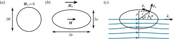
Sketch of a ferrofluid drop in the absence (a) and presence (b) of an external uniform magnetic field
 $\boldsymbol{H}_{0}$
. The drop elongates axisymmetrically along the direction of
 $\boldsymbol{H}_{0}$
. (c) Magnetic field lines around the deformed ferrofluid drop (lower half), and parametrization of the drop shape (top half).

2 Theoretical description
We consider a Newtonian and incompressible ferrofluid drop of radius
 $R$
and viscosity
 $\unicode[STIX]{x1D702}_{d}$
immersed in a Newtonian and incompressible fluid of viscosity
 $\unicode[STIX]{x1D702}_{m}$
. For simplicity, we assume any anisotropy in ferrofluid viscosity to be negligible, which is the case in most ferrofluids at low enough ferromagnetic nanoparticle concentrations (Shliomis Reference Shliomis1972). Upon the application of a spatially uniform external magnetic field
 $\boldsymbol{H}_{0}=H_{0}\hat{\boldsymbol{e}}_{z}$
, the ferrofluid drop magnetizes and deforms axisymmetrically along the direction of the applied field (figure 1). We parametrize the axisymmetric drop shape using cylindrical coordinates and the angle
 $\unicode[STIX]{x1D6FC}$
of the outward normal
 $\hat{\boldsymbol{e}}_{n}$
to the drop surface with the axis of symmetry (
 $\cos \unicode[STIX]{x1D6FC}=\hat{\boldsymbol{e}}_{n}\boldsymbol{\cdot }\hat{\boldsymbol{e}}_{z}$
; figure 1
c). Defining
 $s$
as the arclength along the drop interface, the principle curvatures of the drop interface
 $\unicode[STIX]{x1D705}_{s}$
and
 $\unicode[STIX]{x1D705}_{\unicode[STIX]{x1D719}}$
along the directions
 $\hat{\boldsymbol{e}}_{s}$
and
 $\hat{\boldsymbol{e}}_{\unicode[STIX]{x1D719}}$
read
 $\unicode[STIX]{x1D705}_{s}=\text{d}\unicode[STIX]{x1D6FC}/\text{d}s=\cos \unicode[STIX]{x1D6FC}\,\text{d}\unicode[STIX]{x1D6FC}/\text{d}\unicode[STIX]{x1D70C}$
and
 $\unicode[STIX]{x1D705}_{\unicode[STIX]{x1D719}}=\sin \unicode[STIX]{x1D6FC}/\unicode[STIX]{x1D70C}$
, respectively.
In the low-Reynolds-number limit considered here, the shape and dynamics of the drop result from local stress balance, fluid incompressibility in the bulk and the evolution of the magnetic field
 $\boldsymbol{H}$
, together with boundary conditions for the hydrodynamic and magnetic fields at the drop interface. Local stress balance and fluid incompressibility read
 $$\begin{eqnarray}\displaystyle \unicode[STIX]{x1D735}\boldsymbol{\cdot }(\unicode[STIX]{x1D748}^{h}+\unicode[STIX]{x1D748}^{m})=0,\quad \unicode[STIX]{x1D735}\boldsymbol{\cdot }\boldsymbol{u}=0, & & \displaystyle\end{eqnarray}$$
where
 $\unicode[STIX]{x1D748}^{h}$
and
 $\unicode[STIX]{x1D748}^{m}$
are the hydrodynamic and magnetic stress tensors (defined below), respectively, and
 $\boldsymbol{u}$
is the fluid velocity field. Assuming that the magnetic field relaxes much faster than any other dynamical processes in the system (magnetostatic approximation, valid for dilute ferrofluids), the magnetic field
 $\boldsymbol{H}$
and magnetic flux density
 $\boldsymbol{B}$
follow the magnetostatic equations, namely
 $$\begin{eqnarray}\displaystyle \unicode[STIX]{x1D735}\boldsymbol{\cdot }\boldsymbol{B}=0,\quad \unicode[STIX]{x1D735}\times \boldsymbol{H}=0. & & \displaystyle\end{eqnarray}$$
Stress balance and continuity of velocity, tangential magnetic field and normal magnetic flux density at the drop interface impose the following boundary conditions:
 $$\begin{eqnarray}\displaystyle & \displaystyle [[\hat{\boldsymbol{e}}_{n}\boldsymbol{\cdot }(\unicode[STIX]{x1D748}^{h}+\unicode[STIX]{x1D748}^{m})\boldsymbol{\cdot }\hat{\boldsymbol{e}}_{n}]]=\unicode[STIX]{x1D6FE}(\unicode[STIX]{x1D705}_{s}+\unicode[STIX]{x1D705}_{\unicode[STIX]{x1D719}}), & \displaystyle\end{eqnarray}$$
 $$\begin{eqnarray}\displaystyle & \displaystyle [[\hat{\boldsymbol{e}}_{s}\boldsymbol{\cdot }(\unicode[STIX]{x1D748}^{h}+\unicode[STIX]{x1D748}^{m})\boldsymbol{\cdot }\hat{\boldsymbol{e}}_{n}]]=0, & \displaystyle\end{eqnarray}$$
 $$\begin{eqnarray}\displaystyle & \displaystyle [[\boldsymbol{u}]]=0,\quad \boldsymbol{u}_{int}=(\hat{\boldsymbol{e}}_{n}\boldsymbol{\cdot }\boldsymbol{u})\hat{\boldsymbol{e}}_{n}, & \displaystyle\end{eqnarray}$$
 $$\begin{eqnarray}\displaystyle & \displaystyle [[\boldsymbol{H}\boldsymbol{\cdot }\hat{\boldsymbol{e}}_{s}]]=0,\quad [[\boldsymbol{B}\boldsymbol{\cdot }\hat{\boldsymbol{e}}_{n}]]=0, & \displaystyle\end{eqnarray}$$
where
 $\unicode[STIX]{x1D6FE}$
is the interfacial tension between the ferrofluid and its surrounding medium,
 $\boldsymbol{u}_{int}$
is the interface velocity, and the notation
 $[[x]]\equiv x_{out}-x_{in}$
indicates the discontinuity of the quantity
 $x$
at the interface. The continuity of tangential magnetic field and normal magnetic flux density (2.6) is due to the magnetostatic approximation (no
 $\unicode[STIX]{x1D719}$
component considered due to the axial symmetry).
Given that both the ferrofluid drop and the continuous medium surrounding it are Newtonian fluids, the hydrodynamic stress tensor reads
 $$\begin{eqnarray}\displaystyle \unicode[STIX]{x1D748}^{h}=-P\unicode[STIX]{x1D644}+\unicode[STIX]{x1D702}\dot{\unicode[STIX]{x1D750}}, & & \displaystyle\end{eqnarray}$$
where
 $\unicode[STIX]{x1D644}$
is the unit tensor,
 $P$
the hydrostatic pressure,
 $\unicode[STIX]{x1D702}$
the fluid viscosity (
 $\unicode[STIX]{x1D702}=\unicode[STIX]{x1D702}_{d}$
for the drop and
 $\unicode[STIX]{x1D702}=\unicode[STIX]{x1D702}_{m}$
for the external medium) and
 $\dot{\unicode[STIX]{x1D750}}=(\unicode[STIX]{x1D735}\boldsymbol{u}+\unicode[STIX]{x1D735}\boldsymbol{u}^{\text{T}})/2$
the strain-rate tensor. In the magnetostatic approximation, the magnetic stress inside the ferrofluid drop is given by (Stierstadt & Liu Reference Stierstadt and Liu2015)
 $$\begin{eqnarray}\displaystyle \unicode[STIX]{x1D748}^{m}=-\unicode[STIX]{x1D707}_{0}\left(\frac{1}{2}\boldsymbol{H}^{2}+\int _{0}^{H}\boldsymbol{M}(\boldsymbol{H})\boldsymbol{\cdot }\text{d}\boldsymbol{H}\right)\unicode[STIX]{x1D644}+\boldsymbol{H}\otimes \boldsymbol{B}, & & \displaystyle\end{eqnarray}$$
where
 $\unicode[STIX]{x1D707}_{0}$
is the vacuum magnetic permeability and
 $\boldsymbol{M}$
is the drop magnetization.
Both in the external non-magnetic medium and inside the ferrofluid drop,
 $\unicode[STIX]{x1D735}\boldsymbol{\cdot }\unicode[STIX]{x1D748}^{m}=0$
. In the non-magnetic external medium,
 $\unicode[STIX]{x1D735}\boldsymbol{\cdot }\unicode[STIX]{x1D748}^{m}=-\unicode[STIX]{x1D735}B^{2}/(2\unicode[STIX]{x1D707}_{0})+(\boldsymbol{B}\boldsymbol{\cdot }\unicode[STIX]{x1D735})\boldsymbol{B}/\unicode[STIX]{x1D707}_{0}$
, which vanishes because
 $\unicode[STIX]{x1D735}\times \boldsymbol{B}=0$
. Inside the drop, the term vanishes because the ferrofluid contains dispersed mobile ferromagnetic particles that impose uniform magnetic field and magnetization inside the drop. Furthermore, the magnetic shear stress at the interface, which reads
 $[[\hat{\boldsymbol{e}}_{s}\boldsymbol{\cdot }\unicode[STIX]{x1D748}^{m}\boldsymbol{\cdot }\hat{\boldsymbol{e}}_{n}]]=[[(\boldsymbol{H}\boldsymbol{\cdot }\hat{\boldsymbol{e}}_{s})(\boldsymbol{B}\boldsymbol{\cdot }\hat{\boldsymbol{e}}_{n})]]$
, vanishes because the tangential component of
 $\boldsymbol{H}$
and the normal component of
 $\boldsymbol{B}$
are continuous at the drop interface (2.6). In contrast to ferrofluid drops, in which the normal component of the magnetic flux density is always continuous at the drop interface due to the non-existence of magnetic charges, the analogous continuity is not satisfied for weakly conducting (leaky) dielectric drops under electric fields because of electric charge accumulation at the interface (see Melcher & Taylor (Reference Melcher and Taylor1969) and Saville (Reference Saville1997) for reviews). Under those conditions, the electric shear stress on the interface does not vanish, which results in fluid flows and affects the drop shapes (Lac & Homsy Reference Lac and Homsy2007; Salipante & Vlahovska Reference Salipante and Vlahovska2010; Lanauze, Walker & Khair Reference Lanauze, Walker and Khair2015).
Using the expressions (2.7) and (2.8) for the hydrodynamic and magnetic stress tensors as well as the simplifications described above, equations (2.3) and (2.4) reduce to
 $$\begin{eqnarray}\displaystyle & \displaystyle [[\hat{\boldsymbol{e}}_{n}\boldsymbol{\cdot }\unicode[STIX]{x1D748}^{m}\boldsymbol{\cdot }\hat{\boldsymbol{e}}_{n}]]-[[P]]+[[\unicode[STIX]{x1D702}\hat{\boldsymbol{e}}_{n}\boldsymbol{\cdot }\dot{\unicode[STIX]{x1D750}}\boldsymbol{\cdot }\hat{\boldsymbol{e}}_{n}]]=\unicode[STIX]{x1D6FE}(\unicode[STIX]{x1D705}_{s}+\unicode[STIX]{x1D705}_{\unicode[STIX]{x1D719}}), & \displaystyle\end{eqnarray}$$
 $$\begin{eqnarray}\displaystyle & \displaystyle [[\unicode[STIX]{x1D702}\hat{\boldsymbol{e}}_{s}\boldsymbol{\cdot }\dot{\unicode[STIX]{x1D750}}\boldsymbol{\cdot }\hat{\boldsymbol{e}}_{n}]]=0. & \displaystyle\end{eqnarray}$$
2.1 Scales and dimensionless parameters
We scale all length scales with the radius
 $R$
of the initial undeformed drop, all stresses with the capillary stress scale
 $\unicode[STIX]{x1D70E}_{c}=\unicode[STIX]{x1D6FE}/R$
, and time with the relaxation time scale
 $\unicode[STIX]{x1D70F}_{m}\equiv \unicode[STIX]{x1D702}_{m}/\unicode[STIX]{x1D70E}_{c}$
. Equation (2.9), which embodies the local normal stress balance at the drop interface, can then be expanded and rewritten in the following dimensionless form:
 $$\begin{eqnarray}\displaystyle \unicode[STIX]{x1D6FD}\cos ^{2}\unicode[STIX]{x1D6FC}+Q(\tilde{\unicode[STIX]{x1D70C}})+\hat{\boldsymbol{e}}_{n}\boldsymbol{\cdot }\dot{\tilde{\unicode[STIX]{x1D750}}}_{m}\boldsymbol{\cdot }\hat{\boldsymbol{e}}_{n}-\unicode[STIX]{x1D706}\,\hat{\boldsymbol{e}}_{n}\boldsymbol{\cdot }\dot{\tilde{\unicode[STIX]{x1D750}}}_{d}\boldsymbol{\cdot }\hat{\boldsymbol{e}}_{n}=\frac{\text{d}\unicode[STIX]{x1D6FC}}{\text{d}\tilde{\unicode[STIX]{x1D70C}}}\cos \unicode[STIX]{x1D6FC}+\frac{\sin \unicode[STIX]{x1D6FC}}{\tilde{\unicode[STIX]{x1D70C}}}, & & \displaystyle\end{eqnarray}$$
where the ratio
 $\unicode[STIX]{x1D6FD}\equiv \unicode[STIX]{x1D70E}_{m}/\unicode[STIX]{x1D70E}_{c}$
of the magnetic stress scale
 $\unicode[STIX]{x1D70E}_{m}\equiv \unicode[STIX]{x1D707}_{0}M^{2}(H)/2$
to the capillary stress scale, and the ratio
 $\unicode[STIX]{x1D706}\equiv \unicode[STIX]{x1D702}_{d}/\unicode[STIX]{x1D702}_{m}$
of the fluid viscosities inside and outside the drop, are the only dimensionless parameters in the problem and fully determine its solutions. The variable
 $Q\equiv (\unicode[STIX]{x1D70E}_{i}-[[P]])/\unicode[STIX]{x1D70E}_{c}$
, which corresponds to the normalized sum of the hydrostatic pressure discontinuity at the interface and an isotropic magnetic stress term
 $\unicode[STIX]{x1D70E}_{i}\equiv \unicode[STIX]{x1D707}_{0}\int _{0}^{H}M\,\text{d}H$
, is determined by imposing drop volume conservation and is thus a function of
 $\unicode[STIX]{x1D6FD}$
and
 $\unicode[STIX]{x1D706}$
. Because the surrounding medium is non-magnetic, the magnetic stress,
 $\unicode[STIX]{x1D70E}_{m}$
, depends only on the uniform magnetization and magnetic field inside the drop.
3 Exact equilibrium drop shapes
In equilibrium, the fluid flows inside and outside the drop vanish and the pressure equilibrates inside and outside the drop. In these conditions, equation (2.11) reduces to
 $$\begin{eqnarray}\displaystyle \unicode[STIX]{x1D6FD}\cos ^{2}\unicode[STIX]{x1D6FC}+Q=\frac{\text{d}\unicode[STIX]{x1D6FC}}{\text{d}\tilde{\unicode[STIX]{x1D70C}}}\cos \unicode[STIX]{x1D6FC}+\frac{\sin \unicode[STIX]{x1D6FC}}{\tilde{\unicode[STIX]{x1D70C}}}. & & \displaystyle\end{eqnarray}$$
Solutions of (3.1) depend solely on
 $\unicode[STIX]{x1D6FD}$
, as the viscosity ratio
 $\unicode[STIX]{x1D706}$
does not play any role in the absence of fluid flows. The variable
 $Q$
, now uniform along the interface, is a parameter determined by imposing drop volume conservation and depends only on
 $\unicode[STIX]{x1D6FD}$
.
We obtain the exact equilibrium shapes of the drop for different values of
 $\unicode[STIX]{x1D6FD}$
by numerically integrating (3.1). Starting from nearly spherical shapes for
 $\unicode[STIX]{x1D6FD}\ll 1$
, drops become increasingly deformed as
 $\unicode[STIX]{x1D6FD}$
increases and take approximately ellipsoidal shapes for small to moderate deformations. For large values of
 $\unicode[STIX]{x1D6FD}$
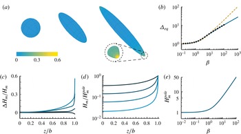
, corresponding to large drop deformations (figure 2
a), drops increasingly deviate from ellipsoidal shapes, especially at their poles, as reported by Sero-Guillaume et al. (Reference Sero-Guillaume, Zouaoui, Bernardin and Brancher1992). We analyse this deviation by calculating the difference
 $\unicode[STIX]{x0394}H_{m}=H_{m}-H_{m}^{ell}$
between the local mean curvature
 $H_{m}$
of the exact equilibrium drop shape and the mean curvature
 $H_{m}^{ell}$
of an ellipsoid with the same semiaxes (figure 2
c). The spatial dependence of the mean curvature and its value at the pole
 $H_{m}^{pole}$
as a function of
 $\unicode[STIX]{x1D6FD}$
are also given in figures 2(d) and 2(e), respectively.
The equilibrium aspect ratio
 $\unicode[STIX]{x1D6E5}_{eq}\equiv b/a$
of the drops, with
 $b$
and
 $a$
being the major and minor semiaxes, respectively, is shown in figure 2(b). These results are in agreement with recent works on electrically deformed drops (Pillai et al.
Reference Pillai, Berry, Harvie and Davidson2015) and show that assuming ellipsoidal drop shapes (dashed line in figures 2
b) results in a significant overestimation of aspect ratio for moderate to large values of
 $\unicode[STIX]{x1D6FD}$
, namely
 $\unicode[STIX]{x1D6FD}\gtrsim 10$
(or aspect ratios
 $\unicode[STIX]{x1D6E5}_{eq}\gtrsim 4$
).
(a) Equilibrium drop shapes for
 $\unicode[STIX]{x1D6FD}=0,10,100$
(left, middle, right). (b) Aspect ratio of equilibrium drop shapes,
 $\unicode[STIX]{x1D6E5}_{eq}$
, as a function of
 $\unicode[STIX]{x1D6FD}$
for the numerically obtained exact drop shapes (solid blue line), assuming an ellipsoidal drop shapes (dashed yellow line), and for the drop shape obtained from simulations (black dots, see next section). (c) Relative deviation
 $\unicode[STIX]{x0394}H_{m}/H_{m}$
of local mean curvature
 $H_{m}$
from that of an ellipsoid for
 $\unicode[STIX]{x1D6FD}=3,10,30,100$
(dark to light), which also corresponds to the colour coding of the drop surface in (a). (d) Spatial dependence of the local mean curvature
 $H_{m}$
normalized by the mean curvature
 $H_{m}^{pole}$
at the pole (
 $z/b=1$
) for
 $\unicode[STIX]{x1D6FD}=3,10,30,100$
(dark to light). (e) Mean curvature at the pole,
 $H_{m}^{pole}$
, as a function of
 $\unicode[STIX]{x1D6FD}$
. For large
 $\unicode[STIX]{x1D6FD}$
,
 $H_{m}^{pole}\approx \unicode[STIX]{x1D6FD}/2$
.

Important insight on how close the exact equilibrium drop shapes are to ellipsoids for small and moderate values of
 $\unicode[STIX]{x1D6FD}\gtrsim 1$
, analysed above numerically by considering the differences in local curvatures, can be gained by analytical analysis. Specifically, we expand the shape function
 $\tilde{r}$
in terms of the spherical harmonics
 $Y_{\ell }^{m}(\unicode[STIX]{x1D703},\unicode[STIX]{x1D719})$
, where
 $\tilde{r}\equiv r/R$
,
 $\unicode[STIX]{x1D703}$
and
 $\unicode[STIX]{x1D719}$
are the dimensionless radial distance, polar angle and azimuthal angle, with respect to the centre of the drop. Such expansions have been employed in previous works to study the dynamics of drops under sudden increase or decrease, as well as oscillations, of electric fields (Basaran et al.
Reference Basaran, Patzek, Benner and Scriven1995), the motion of bubbles in inviscid fluids (Meiron Reference Meiron1989; Kushch et al.
Reference Kushch, Sangani, Spelt and Koch2002) and the stability of bubbles under electric fields (Shaw & Spelt Reference Shaw and Spelt2009). Owing to the axial and mirror symmetry of the drop, the expansion must be
 $\unicode[STIX]{x1D719}$
-independent, and consist only of
 $m=0$
and even
 $\ell =2j$
modes, where
 $j$
is a non-negative integer. Therefore,
 $\tilde{r}(\unicode[STIX]{x1D703})=1+\sum _{j=0}^{\infty }y_{2j}(\unicode[STIX]{x1D6FD})Y_{2j}^{0}(\unicode[STIX]{x1D703})$
, where the coefficients
 $y_{2j}$
are zero when
 $\unicode[STIX]{x1D6FD}=0$
. Truncating the series at
 $j=3$
and expanding the coefficients
 $y_{2j}(\unicode[STIX]{x1D6FD})$
up to third order in
 $\unicode[STIX]{x1D6FD}$
, the normal stress balance (equation (3.1) rewritten in spherical coordinates) and drop volume conservation yield
 $$\begin{eqnarray}\displaystyle \tilde{r}(\unicode[STIX]{x1D703}) & \simeq & \displaystyle 1+\frac{\sqrt{\unicode[STIX]{x03C0}}}{90}\left(-\unicode[STIX]{x1D6FD}^{2}+\frac{2}{63}\unicode[STIX]{x1D6FD}^{3}\right)Y_{0}^{0}(\unicode[STIX]{x1D703})+\frac{1}{3}\sqrt{\frac{\unicode[STIX]{x03C0}}{5}}\left(\unicode[STIX]{x1D6FD}-\frac{1}{42}\unicode[STIX]{x1D6FD}^{2}-\frac{8}{315}\unicode[STIX]{x1D6FD}^{3}\right)Y_{2}^{0}(\unicode[STIX]{x1D703})\nonumber\\ \displaystyle & & \displaystyle +\,\frac{13\sqrt{\unicode[STIX]{x03C0}}}{945}\left(\unicode[STIX]{x1D6FD}^{2}-\frac{9}{286}\unicode[STIX]{x1D6FD}^{3}\right)Y_{4}^{0}(\unicode[STIX]{x1D703})+\left(\sqrt{\frac{\unicode[STIX]{x03C0}}{13}}\frac{197}{41\,580}\unicode[STIX]{x1D6FD}^{3}\right)Y_{6}^{0}(\unicode[STIX]{x1D703}).\end{eqnarray}$$
All spherical harmonics up to order
 $\ell =6$
have amplitudes of order
 $\unicode[STIX]{x1D6FD}^{2}$
or higher with small numerical coefficients, except for the ellipsoidal mode
 $\ell =2$
, which has an amplitude of order
 $\unicode[STIX]{x1D6FD}$
. Comparison of the
 $\unicode[STIX]{x1D6FD}$
-dependent coefficients (up to
 $\ell =6$
) indicates that it is safe to assume ellipsoidal drop shapes for
 $\unicode[STIX]{x1D6FD}\lesssim 5$
. Major deviations of the ellipsoidal shape start occurring at
 $\unicode[STIX]{x1D6FD}\simeq 10$
(corresponding to aspect ratios
 ${\sim}4$
), which agrees with our numerical calculations and simulations (figure 2
c).
3.1 Equilibrium drop shape as a function of the externally applied magnetic field
So far we have discussed the equilibrium drop shapes as a function of
 $\unicode[STIX]{x1D6FD}$
, the ratio of magnetic stress to the capillary stress scale. This analysis is generic, as it does not involve the specific magnetic properties of the ferrofluid. However, some interesting aspects of drop deformations are revealed when drop deformations are analysed as a function of the experimentally controlled external magnetic field
 $H_{0}$
and the specific magnetic properties of the ferrofluid. It is known, for instance, that above a certain threshold of relative magnetic permeability (permittivity) of the drop to the medium, drop shapes become bistable for a range of magnetic (electric) fields (Taylor Reference Taylor1964; Rosenkilde Reference Rosenkilde1969; Miksis Reference Miksis1981; Bacri & Salin Reference Bacri and Salin1982; Wohlhuter & Basaran Reference Wohlhuter and Basaran1992). These studies also show that, for dielectric drops, equilibrium solutions cease to exist altogether above a certain threshold of relative permittivity and electric field, effectively making large deformations unstable for drops with high permittivity. This instability results from the formation of conical poles (Sherwood Reference Sherwood1991; Li et al.
Reference Li, Halsey and Lobkovsky1994; Stone et al.
Reference Stone, Lister and Brenner1999) due to the divergence of the electric field just outside the drop at the poles.
To study these effects in magnetically actuated ferrofluid drops, we analyse the deformations of nonlinear ferrofluid drops as a function of the externally applied uniform magnetic field. In order to obtain the equilibrium drop shapes as a function of the applied field, it is necessary to know the dependence of the magnetization
 $M$
of the specific ferrofluid used on the applied magnetic field. The ferromagnetic properties of the ferrofluid depend on the physicochemical properties of the magnetic nanoparticles dispersed in the drop phase. In the absence of hysteresis (small interaction energy between nanoparticles), the ferrofluid drop can be effectively described by its magnetization
 $M(H)=M_{s}\,\mathscr{L}(H/H_{c})$
, where
 $H$
is the magnetic field inside the drop and
 $M_{s}$
and
 $H_{c}$
are the saturation magnetization and the saturating field, respectively. In what follows, we assume Langevin magnetization,
 $\mathscr{L}(x)\equiv \coth x-1/x$
(Rosensweig Reference Rosensweig2013), which describes accurately ferrofluids with monodisperse magnetic particles. This function also captures qualitatively the behaviour of more general cases of polydisperse magnetic particles, where the magnetization relation is found by integrating over multiple Langevin functions, which correspond to the particle sizes present in the ferrofluid (Zimny et al.
Reference Zimny, Mascaro, Brunet, Poncelet, Aristégui, Leng, Sandre and Mondain-Monval2014). As the volume fraction of particles and the interaction energy per volume between particles increase, hysteresis effects appear and the applicability of the Langevin model becomes more limited. The effects of hysteresis in the ferrofluid magnetization on the drop shapes and dynamics are not studied here and are left to future work.
The magnetization
 $M$
of the drop is a function of the magnetic field
 $H=H_{0}+H_{in}$
inside the drop, where the induced magnetic field
 $H_{in}=-kM$
depends on the magnetic field
 $H$
via
 $M$
and the drop shape-dependent demagnetization factor
 $k$
, which is maximal (
 $k=1/3$
) for spherical drops and decreases monotonically for increasing drop deformations. The magnetic field in the drop,
 $H=H_{0}-kM_{s}\,\mathscr{L}(H/H_{c})$
, is thus given implicitly as a function of the external magnetic field
 $H_{0}$
and the demagnetization factor
 $k$
, which we have calculated numerically for the exact equilibrium drop shapes using standard methods (Landau, Pitaevskii & Lifshitz Reference Landau, Pitaevskii and Lifshitz1984). This implicit relation introduces a dimensionless parameter
 $\unicode[STIX]{x1D707}\equiv M_{s}/H_{c}$
, which depends only on the properties of the ferrofluid. While equilibrium drop shapes depend uniquely on
 $\unicode[STIX]{x1D6FD}$
, relating these shapes to
 $H_{0}$
requires two parameters, namely,
 $\unicode[STIX]{x1D707}$
and
 $\unicode[STIX]{x1D6FD}_{s}\equiv \unicode[STIX]{x1D707}_{0}M_{s}^{2}R/2\unicode[STIX]{x1D6FE}$
, where
 $\unicode[STIX]{x1D6FD}_{s}$
is the maximal value of
 $\unicode[STIX]{x1D6FD}=\unicode[STIX]{x1D6FD}_{s}\,\mathscr{L}^{2}(H/H_{c})$
at the saturation magnetization of the ferrofluid.
Equilibrium aspect ratio
 $\unicode[STIX]{x1D6E5}_{eq}$
as a function of
 $H_{0}/H_{c}$
for
 $\unicode[STIX]{x1D707}=1,10,100,1000$
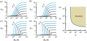
(a, b, c, d, respectively), where
 $\unicode[STIX]{x1D707}=M_{s}/H_{c}$
is the ratio of saturation magnetization to saturation field. For each value of
 $\unicode[STIX]{x1D707}$
, solutions for values of
 $\unicode[STIX]{x1D6FD}_{s}=3,10,30,100,300,1000$
are shown, with the lower curves corresponding to smaller
 $\unicode[STIX]{x1D6FD}_{s}$
. (e) Parameter space indicating the region of drop shape bistability.

In figure 3 we show the dependence of the equilibrium drop aspect ratio on the externally applied magnetic field
 $H_{0}$
for different values of
 $\unicode[STIX]{x1D707}$
and
 $\unicode[STIX]{x1D6FD}_{s}$
. For small enough values of
 $\unicode[STIX]{x1D707}$
(figure 3
a,b), the aspect ratio increases monotonically with the applied magnetic field
 $H_{0}$
, and saturates for large values of
 $H_{0}/H_{c}$
, as the magnetization saturates in this limit and so does the magnetic stress. As
 $\unicode[STIX]{x1D707}$
is increased above a critical value, there exist values of
 $\unicode[STIX]{x1D6FD}_{s}$
for which there is a bistability of drop shapes within a range of values of the applied magnetic field
 $H_{0}$
(figure 3
c,d). The range of the parameters
 $\unicode[STIX]{x1D707}$
and
 $\unicode[STIX]{x1D6FD}_{s}$
for which drop shape bistability occurs is shown in figure 3(e). No shape bistability exists below a critical value of
 $\unicode[STIX]{x1D707}$
. While there are qualitative differences between the linear and nonlinear ferrofluid regimes (as also noted by Basaran & Wohlhuter (Reference Basaran and Wohlhuter1992)), the bistability threshold of
 $\unicode[STIX]{x1D707}$
is analogous to the bistability threshold of permeability and permittivity for linear ferrofluid (Bacri & Salin Reference Bacri and Salin1982) and dielectric (Rosenkilde Reference Rosenkilde1969; Miksis Reference Miksis1981; Wohlhuter & Basaran Reference Wohlhuter and Basaran1992) drops, respectively.
The shape bistability diagram in figure 3(e) can be explored experimentally using ferrofluids composed of monodisperse magnetic nanoparticles. Varying the size and volume fraction of the nanoparticles enables controlled changes of the parameter
 $\unicode[STIX]{x1D707}$
through its dependence on
 $H_{c}$
and
 $M_{s}$
, respectively (see Rosensweig (Reference Rosensweig2013) for more details on the Langevin ferrofluid parameters). The parameter
 $\unicode[STIX]{x1D6FD}_{s}$
can be varied independently of
 $\unicode[STIX]{x1D707}$
by changing the radius
 $R$
of the drop, without changing the properties of the ferrofluid.
Regardless of the specific ferrofluid used, no instability due to sharp conical tips is observed in our solutions. This is because, in the limit of non-magnetic media considered here, the magnetic stress is independent of the large field outside the drop at the poles and remains finite (see (3.1)). However, dynamic Rayleigh-type instabilities may cause drop breakups when deformations are large (Sherwood Reference Sherwood1988; Basaran et al. Reference Basaran, Patzek, Benner and Scriven1995; Potts et al. Reference Potts, Barrett and Diver2001; Lac & Homsy Reference Lac and Homsy2007; Afkhami et al. Reference Afkhami, Renardy, Renardy, Riffle and St Pierre2008; Paknemat et al. Reference Paknemat, Pishevar and Pournaderi2012). Also, the drop–medium interface may be destabilized for large enough magnetic fields (Boudouvis et al. Reference Boudouvis, Puchalla, Scriven and Rosensweig1987). We have not studied these instabilities in this work.
Dependence of the equilibrium drop aspect ratio on the externally applied field
 $H_{0}$
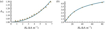
for low (a) and high (b) magnetic fields. Triangles show the measured values obtained by Afkhami et al. (Reference Afkhami, Tyler, Renardy, Renardy, St Pierre, Woodward and Riffle2010) and solid curves show fits to these data obtained from our theoretical analysis (solutions of (3.1)), using the magnetization curves reported in Afkhami et al. (Reference Afkhami, Tyler, Renardy, Renardy, St Pierre, Woodward and Riffle2010) (
 $M=0.8903H+0.1634$
for the linear magnetization regime (a) and
 $M=4.8568\ln (H)-3.956$
for the nonlinear magnetization regime (b), both in
 $\text{kA}~\text{m}^{-1}$
). Using the unperturbed drop radius
 $R=1.291~\text{mm}$
reported by Afkhami et al. (Reference Afkhami, Tyler, Renardy, Renardy, St Pierre, Woodward and Riffle2010), the values of interfacial tension obtained from the fits are
 $\unicode[STIX]{x1D6FE}=18.2~\text{mN}~\text{m}^{-1}$
and
 $\unicode[STIX]{x1D6FE}=17.5~\text{mN}~\text{m}^{-1}$
for the low (a) and high (b) magnetic fields.

3.2 Comparison of equilibrium deformations with previous experiments
Various experimental works have studied the deformation of ferrofluid drops as a function of experimentally controlled parameters, such as the applied magnetic field. To explore the importance of considering the exact drop shapes and also to address discrepancies between previous theoretical and experimental results, we compare our numerical predictions to experimental observations of equilibrium drop deformation in both linear and nonlinear ferrofluid regimes by Afkhami et al. (Reference Afkhami, Tyler, Renardy, Renardy, St Pierre, Woodward and Riffle2010). The theoretical description in Afkhami et al. (Reference Afkhami, Tyler, Renardy, Renardy, St Pierre, Woodward and Riffle2010) was able to accurately reproduce the observed dependence of the drop aspect ratio with the applied magnetic field for small magnetic fields (small deformations) assuming ellipsoidal drop shapes. However, for large magnetic fields (large deformations), the measured dependence of the drop aspect ratio on the applied magnetic field could not be explained by the theoretical or numerical results of that work, even when ad hoc assumptions, such as a field-dependent interfacial tension
 $\unicode[STIX]{x1D6FE}$
, were considered. We re-evaluate this discrepancy in Afkhami et al. (Reference Afkhami, Tyler, Renardy, Renardy, St Pierre, Woodward and Riffle2010) using our theoretical description, which does not assume ellipsoidal drop shapes and accounts for the exact drop shape.
Figures 4(a) and 4(b) show the dependence of the drop aspect ratio on the applied magnetic field measured by Afkhami et al. (Reference Afkhami, Tyler, Renardy, Renardy, St Pierre, Woodward and Riffle2010), together with our numerical results, which were computed using the magnetization curves measured in Afkhami et al. (Reference Afkhami, Tyler, Renardy, Renardy, St Pierre, Woodward and Riffle2010). Importantly, fitting the experimental data independently in the linear and nonlinear regimes of the ferrofluid (using the value of unperturbed drop radius reported in Afkhami et al. (Reference Afkhami, Tyler, Renardy, Renardy, St Pierre, Woodward and Riffle2010)), we obtain the same value of the drop interfacial tension. Specifically, the values of the interfacial tension obtained from the fits are
 $\unicode[STIX]{x1D6FE}=18.2~\text{mN}~\text{m}^{-1}$
and
 $\unicode[STIX]{x1D6FE}=17.5~\text{mN}~\text{m}^{-1}$
for the low- and high-magnetic-field regimes, respectively, which differ by roughly
 $3\,\%$
and are well within the experimental errors in Afkhami et al. (Reference Afkhami, Tyler, Renardy, Renardy, St Pierre, Woodward and Riffle2010). Our theoretical description is thus able to reproduce the experimental data for both low and high magnetic fields (linear and nonlinear magnetization regimes) using a single value of the interfacial tension. Our analysis indicates that the discrepancy between theoretical predictions and observations at large values of the magnetic field in Afkhami et al. (Reference Afkhami, Tyler, Renardy, Renardy, St Pierre, Woodward and Riffle2010) was due to the ellipsoidal shape approximation.
4 Dynamics of ferrofluid drop deformation
In contrast to the equilibrium drop shapes, the dynamics of ferrofluid drop deformations involves fluid flows inside and outside the drop and, therefore, it depends on both
 $\unicode[STIX]{x1D6FD}$
and the viscosity ratio
 $\unicode[STIX]{x1D706}$
. The equations that govern the dynamics of drop shape deformation and fluid flows in the system were derived in § 2 ((2.1)–(2.5)). Analytical treatment of this free boundary problem is complex and only possible in some limiting regimes. Instead, we numerically integrate them using the Two Phase Fluid Moving Mesh module of COMSOL Multiphysics V5.0. We use a hybrid approach and solve numerically only for the hydrodynamic fields by including the analytical values of the magnetic stresses
 $\unicode[STIX]{x1D70E}_{m}\cos ^{2}\unicode[STIX]{x1D6FC}$
and
 $\unicode[STIX]{x1D70E}_{i}$
(see § 2) as normal stresses at the drop interface. We have checked that this hybrid method yields the same results as the full numerical solution including both magnetic and hydrodynamic fields, but it is considerably better in terms of computational efficiency. In addition to significantly reducing the simulation time, this approach also reduces numerical errors and instabilities by using a smooth analytical function for the magnetic stress at the drop interface.
4.1 Dynamics of drop relaxation
We consider first an initially deformed drop that relaxes towards its final equilibrium spherical shape. Such drop relaxation in the absence of any magnetic field corresponds to
 $\unicode[STIX]{x1D6FD}=0$
and, therefore, relaxation dynamics depends solely on the viscosity ratio
 $\unicode[STIX]{x1D706}$
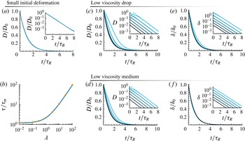
. To allow meaningful comparisons with previous theoretical works, which assumed ellipsoidal drop shapes (Rallison Reference Rallison1984), we consider, in this section, the drop relaxation from an ellipsoidal shape. We have checked that the results shown below do not change qualitatively if the initial drop shape is set to its exact equilibrium shape (under a magnetic field) instead of an ellipsoid. In particular, the changes are negligible for small and moderate values of
 $\unicode[STIX]{x1D6FD}$
, as the equilibrium drop shapes are close to ellipsoids in this limit (figure 2).
(a) Time evolution of the deformation factor
 $D(t)$
for a drop relaxing towards its final spherical state starting from a barely deformed initial ellipsoidal drop (
 $D_{0}\approx 0.091$
or
 $\unicode[STIX]{x1D6E5}_{0}=1.2$
) for viscosity ratio
 $\unicode[STIX]{x1D706}=10^{-2}{-}10^{2}$
, and (b) their decay time scales
 $\unicode[STIX]{x1D70F}$
as a function of
 $\unicode[STIX]{x1D706}$
. Solid line and points in (b) correspond to the theoretical result (
 $\unicode[STIX]{x1D70F}_{R}=\unicode[STIX]{x1D70F}_{m}(2\unicode[STIX]{x1D706}+3)(19\unicode[STIX]{x1D706}+16)/(40(\unicode[STIX]{x1D706}+1))$
; Rallison (Reference Rallison1984)), and our numerical value of
 $\unicode[STIX]{x1D70F}$
, respectively. (c,d) Plots of
 $D(t)$
for finite initial deformations:
 $D_{0}\approx 0.007{-}0.47$
for (c)
 $\unicode[STIX]{x1D706}\ll 1$
and (d)
 $\unicode[STIX]{x1D706}\gg 1$
. (e,f) Plots of
 $\unicode[STIX]{x1D6FF}(t)$
of the same simulations as in (c) and (d) with initial values
 $\unicode[STIX]{x1D6FF}_{0}\approx 0.014{-}3.5$
for (e)
 $\unicode[STIX]{x1D706}\ll 1$
and (f)
 $\unicode[STIX]{x1D706}\gg 1$
.

Figure 5 shows the time evolution of the drop deformation, quantified by their deformation factor
 $D\equiv (b-a)/(b+a)$
(Rallison Reference Rallison1984), during relaxation towards the spherical equilibrium shape, for different values of initial deformation
 $D_{0}$
and
 $\unicode[STIX]{x1D706}$
. For small initial drop deformations (figure 5
a), the deformation factor
 $D$
decays exponentially with a
 $\unicode[STIX]{x1D706}$
-dependent relaxation time scale
 $\unicode[STIX]{x1D70F}_{R}$
(figure 5
b). Our numerical results agree perfectly with the analytical prediction
 $\unicode[STIX]{x1D70F}_{R}(\unicode[STIX]{x1D706})=\unicode[STIX]{x1D70F}_{m}(2\unicode[STIX]{x1D706}+3)(19\unicode[STIX]{x1D706}+16)/(40(\unicode[STIX]{x1D706}+1))$
for drop relaxation from small initial deformations (Rallison Reference Rallison1984, figure 5
b). As the initial drop deformation becomes finite, the decay of deformation factor
 $D(t)$
deviates from the exponential decay as long as the drop shape deformations remain finite. Once drop deformation reaches small enough values,
 $D(t)$
decays exponentially with the same
 $D_{0}$
-independent time scale
 $\unicode[STIX]{x1D70F}_{R}$
(figure 5
c,d, insets). While
 $D(t)$
deviates substantially from a single-exponential decay for even mild deformations (
 $D\gtrsim 0.1$
or
 $\unicode[STIX]{x1D6E5}\gtrsim 1.2$
), the quantity
 $\unicode[STIX]{x1D6FF}\equiv b/a-1$
displays an exponential decay with the same characteristic time scale
 $\unicode[STIX]{x1D70F}_{R}$
for significantly larger initial drop deformations (figure 5
e,f), especially for relatively low-viscosity external media (
 $\unicode[STIX]{x1D706}\gg 1$
).
4.2 Dynamics of drop deformation from an initially undeformed spherical shape
We simulate an initially undeformed spherical ferrofluid drop actuated at time
 $t=0$
with a spatially uniform magnetic field and analyse the dynamics of its deformation towards its equilibrium deformed shape (equilibrium deformation obtained in simulations shown as black dots in figure 2
c). The actuation dynamics, which we analyse below using the quantity
 $\unicode[STIX]{x1D6FF}(t)$
(equivalent to the drop aspect ratio), depends on both
 $\unicode[STIX]{x1D6FD}$
and
 $\unicode[STIX]{x1D706}$
.
For small values of
 $\unicode[STIX]{x1D6FD}$
, corresponding to small final (equilibrium) drop deformations, the dynamics of drop deformation is exponential, namely
 $\unicode[STIX]{x1D6FF}(t)\simeq (\unicode[STIX]{x1D6FD}/4)(1-\exp (t/\unicode[STIX]{x1D70F}_{R}))$
, where
 $\unicode[STIX]{x1D70F}_{R}$
is the
 $\unicode[STIX]{x1D6FD}$
-independent relaxation time scale obtained previously for drop relaxations (figure 5
b), and
 $\unicode[STIX]{x1D6FD}/4$
is the equilibrium deformation for small values of
 $\unicode[STIX]{x1D6FD}$
(from (3.2) or from Tsebers (Reference Tsebers1985)). This is due to a negligible change in the magnetic stress during deformation, time reversibility of Stokes flow and the nearly spherical final drop shape for small applied magnetic field (small
 $\unicode[STIX]{x1D6FD}$
).
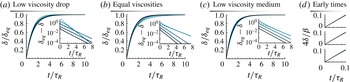
Time evolution of
 $\unicode[STIX]{x1D6FF}(t)$
in the saturation magnetization regime for various values of
 $\unicode[STIX]{x1D6FD}_{s}=0.28,~0.80,~2.3,~9.1$
(darker colour corresponds to smaller
 $\unicode[STIX]{x1D6FD}_{s}$
) and (a)
 $\unicode[STIX]{x1D706}\ll 1$
, (b)
 $\unicode[STIX]{x1D706}=1$
and (c)
 $\unicode[STIX]{x1D706}\gg 1$
. The insets show
 $\unicode[STIX]{x1D6FF}_{eq}-\unicode[STIX]{x1D6FF}(t)$
versus time in log scale with the fitted exponentials at long times (dashed lines). (d) Same
 $\unicode[STIX]{x1D6FF}(t)$
curves normalized with
 $\unicode[STIX]{x1D6FD}_{s}/4$
at early times
 $t\ll \unicode[STIX]{x1D70F}_{R}$
.

For larger values of
 $\unicode[STIX]{x1D6FD}$
, the exponential relation above only holds for
 $t\ll \unicode[STIX]{x1D70F}_{R}$
(while the drop deformations are still relatively small), leading to the linear relation
 $\unicode[STIX]{x1D6FF}(t)\simeq (\unicode[STIX]{x1D6FD}/4)(t/\unicode[STIX]{x1D70F}_{R})$
at early times (figure 6
d). Specifically,
 $$\begin{eqnarray}\displaystyle \unicode[STIX]{x1D6FF}(t)\simeq \frac{10(\unicode[STIX]{x1D706}+1)}{(2\unicode[STIX]{x1D706}+3)(19\unicode[STIX]{x1D706}+16)}\frac{t}{(\unicode[STIX]{x1D702}_{m}/\unicode[STIX]{x1D70E}_{m})}, & & \displaystyle\end{eqnarray}$$
which is independent of the capillary stresses because the drop deformation is much smaller than its equilibrium value
 $\unicode[STIX]{x1D6FF}_{eq}$
at these early times, and the restoring capillary stresses are small compared to the magnetic stresses. As time goes on, the droplet gets increasingly deformed and
 $\unicode[STIX]{x1D6FF}(t)$
crosses over to another exponential regime with a
 $\unicode[STIX]{x1D6FD}$
- and
 $\unicode[STIX]{x1D706}$
-dependent time scale
 $\unicode[STIX]{x1D70F}$
as it approaches its (final) equilibrium state (figure 6, insets). The time scale
 $\unicode[STIX]{x1D70F}$
of this final exponential approach depends on both
 $\unicode[STIX]{x1D706}$
and
 $\unicode[STIX]{x1D6FD}$
only for large
 $\unicode[STIX]{x1D6FD}$
and, therefore,
 $\unicode[STIX]{x1D70F}$
deviates from
 $\unicode[STIX]{x1D70F}_{R}$
only when the final equilibrium drop shape deviates substantially from spherical. To analyse the changes of the time scale
 $\unicode[STIX]{x1D70F}$
to reach the final equilibrium drop shape, we study the ratio
 $\unicode[STIX]{x1D70F}/\unicode[STIX]{x1D70F}_{R}$
for distinct regimes of the ferrofluid and limiting viscosity ratios
 $\unicode[STIX]{x1D706}$
(figure 7).
As mentioned in § 3.1, the relation between the magnetization of a Langevin ferrofluid and the applied field
 $H_{0}$
involves two dimensionless parameters, namely,
 $\unicode[STIX]{x1D6FD}_{s}=\unicode[STIX]{x1D707}_{0}M_{s}^{2}R/2\unicode[STIX]{x1D6FE}$
and
 $\unicode[STIX]{x1D707}=M_{s}/H_{c}$
. Therefore, for an arbitrary field, which can span the full nonlinear regime of the magnetization curve of the ferrofluid, the dynamics of drop deformation is controlled by all the dimensionless parameters
 $\unicode[STIX]{x1D706}$
,
 $\unicode[STIX]{x1D6FD}_{s}$
and
 $\unicode[STIX]{x1D707}$
, as well as by the value of the external magnetic field
 $H_{0}$
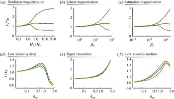
. Figure 7(a) shows the dependence of the normalized time scale
 $\unicode[STIX]{x1D70F}/\unicode[STIX]{x1D70F}_{R}$
on the applied magnetic field
 $H_{0}$
, for different values of
 $\unicode[STIX]{x1D707}$
and
 $\unicode[STIX]{x1D6FD}_{s}$
and limiting regimes of
 $\unicode[STIX]{x1D706}$
. We restrict our analysis to a fixed value
 $\unicode[STIX]{x1D707}\sim 1$
for simplicity and to avoid complications due to the bistability of equilibrium shapes (see § 3.1). We have checked that the results are qualitatively the same for other values of
 $\unicode[STIX]{x1D707}$
, as long as
 $\unicode[STIX]{x1D707}\sim 1$
.
(a–c) Normalized time scale
 $\unicode[STIX]{x1D70F}/\unicode[STIX]{x1D70F}_{R}$
of the final approach of the drops to their deformed equilibrium shapes as a function of
 $H_{0}/H_{c}$
,
 $\unicode[STIX]{x1D6FD}_{0}$
and
 $\unicode[STIX]{x1D6FD}_{s}$
for (a) nonlinear, (b) linear and (c) saturation ferrofluid regimes, and
 $\unicode[STIX]{x1D706}\ll 1$
(squares),
 $\unicode[STIX]{x1D706}=1$
(triangles) and
 $\unicode[STIX]{x1D706}\gg 1$
(circles). A smooth cubic spline curve passes through the points. (d–f) Normalized time scale
 $\unicode[STIX]{x1D70F}/\unicode[STIX]{x1D70F}_{R}$
as a function of the final equilibrium drop deformation
 $\unicode[STIX]{x1D6FF}_{eq}$
for the limiting cases (d)
 $\unicode[STIX]{x1D706}\ll 1$
, (e)
 $\unicode[STIX]{x1D706}=1$
and (f)
 $\unicode[STIX]{x1D706}\gg 1$
. Saturation, linear and nonlinear ferrofluid regimes correspond to squares, triangles and circles, respectively.

For small enough applied magnetic fields (
 $H_{0}\ll H_{c}$
), the drop magnetization
 $M=\unicode[STIX]{x1D712}H$
increases linearly with the magnetic field
 $H$
in the drop (and consequently with the applied field
 $H_{0}$
), where
 $\unicode[STIX]{x1D712}=\unicode[STIX]{x1D707}/3$
is the magnetic susceptibility. In this linear regime, the dynamics of drop deformation depends only on
 $\unicode[STIX]{x1D706}$
,
 $\unicode[STIX]{x1D707}=3\unicode[STIX]{x1D712}$
and the ‘Bond number’
 $\unicode[STIX]{x1D6FD}_{0}\equiv \unicode[STIX]{x1D707}_{0}H_{0}^{2}R/2\unicode[STIX]{x1D6FE}$
(Afkhami et al.
Reference Afkhami, Tyler, Renardy, Renardy, St Pierre, Woodward and Riffle2010), which is equivalent to the applied field
 $H_{0}$
. Figure 7(b) shows the dependence of
 $\unicode[STIX]{x1D70F}/\unicode[STIX]{x1D70F}_{R}$
on
 $\unicode[STIX]{x1D6FD}_{0}$
for limiting cases of
 $\unicode[STIX]{x1D706}$
and fixed
 $\unicode[STIX]{x1D707}\sim 1$
.
For large applied magnetic fields (
 $H_{0}\gg H_{c}$
), the drop magnetization saturates to the value
 $M_{s}$
and remains constant during the drop deformation. In this saturation regime, the time scale
 $\unicode[STIX]{x1D70F}$
is independent of
 $H_{0}$
and depends only on
 $\unicode[STIX]{x1D706}$
and
 $\unicode[STIX]{x1D6FD}_{s}$
. Figure 7(c) shows the dependence of
 $\unicode[STIX]{x1D70F}/\unicode[STIX]{x1D70F}_{R}$
on
 $\unicode[STIX]{x1D6FD}_{s}$
for different limiting cases of the viscosity ratio
 $\unicode[STIX]{x1D706}$
.
In all ferrofluid regimes (saturation, linear and nonlinear), the deviation of
 $\unicode[STIX]{x1D70F}$
from
 $\unicode[STIX]{x1D70F}_{R}$
is of order one for a wide range of equilibrium drop deformations and viscosity ratios
 $\unicode[STIX]{x1D706}$
, indicating that the characteristic time scale of drop deformation towards the equilibrium shape is essentially determined by
 $\unicode[STIX]{x1D70F}_{R}$
. In the cases where either the drop or the external medium have relatively low viscosity (figure 7
d,f), the deviation of
 $\unicode[STIX]{x1D70F}$
from
 $\unicode[STIX]{x1D70F}_{R}$
is smallest, whereas in the intermediate regime (figure 7
e), in which the two fluids have the same viscosity (
 $\unicode[STIX]{x1D706}=1$
), the deviations are largest. The time scale
 $\unicode[STIX]{x1D70F}$
depends only weakly on the specific ferrofluid regime and is essentially determined by the final deformation
 $\unicode[STIX]{x1D6FF}_{eq}$
of the drop, which is controlled by the ratio of magnetic to capillary stresses
 $\unicode[STIX]{x1D6FD}_{s}$
and the value of the magnetic field, as described above(figure 7
d–f).
5 Discussion
In this work, we provided a systematic analysis of the deformation dynamics of a Newtonian ferrofluid drop in a viscous fluid when actuated by spatially uniform magnetic fields. We solved for the exact equilibrium drop shapes as a function of the only relevant dimensionless parameter in the problem, namely the ratio
 $\unicode[STIX]{x1D6FD}$
of magnetic to capillary stresses, for arbitrary physicochemical properties of the ferrofluids. We showed that drop shapes are nearly ellipsoidal for small to intermediate values of
 $\unicode[STIX]{x1D6FD}$
, but that these deviate significantly from ellipsoidal shapes as
 $\unicode[STIX]{x1D6FD}$
is increased, specially at the drop tips. We also showed that the dependence of the equilibrium drop shape on the externally applied magnetic field shows a shape bistability, as previously reported, but only for highly susceptible ferrofluids that are rarely used in most practical applications. In addition, we solve the dynamics of ferrofluid drop deformations in viscous Newtonian fluids when actuated by uniform magnetic fields. The dynamics is obtained for arbitrary ferrofluids (nonlinear and linear magnetizations) as well as for finite drop deformations. We show that the dynamics of drop deformation by an applied uniform magnetic field is controlled by the same time scale as the drop relaxation in the absence of magnetic field, up to a numerical factor that essentially depends on the viscosity ratio and the ratio of magnetic stress to capillary stress. These results were obtained with a computational scheme that we developed using COMSOL Multiphysics V5.0 and allows computationally efficient simulations of the drop dynamics under various conditions. The versatility of this computational scheme will enable the study of ferrofluid drop actuation in a wide range of situations, from viscoelastic fluids to diverse temporal magnetic actuations of the drops.
Our results can be used for many practical applications requiring a detailed understanding of ferrofluid drop dynamics, including biomedical applications such as drug delivery (Gupta & Gupta Reference Gupta and Gupta2005; Bychkova et al. Reference Bychkova, Sorokina, Rosenfeld and Kovarski2012), where shape-dependent particle uptake has been observed (Champion & Mitragotri Reference Champion and Mitragotri2006). Also, precise measurements of the drop dynamics and equilibrium shapes would enable precise local measurements of both the viscosity of the external medium (or the drop) and the drop interfacial tension.
Acknowledgements
We thank G. Leal for fruitful discussions. P.R. thanks the Santa Barbara Foundation and the Errett Fisher Foundation for financial support.