1. INTRODUCTION
Accurate positioning of surface and airborne vehicles such as ships and airplanes is possible using Global Navigation Satellite Systems (GNSS) such as the Global Positioning System (GPS) (Grenon et al., Reference Grenon, An, Smith and Healy2001). However, since GPS signals do not penetrate beneath the water, this system cannot be used in underwater vehicles (Yun et al., Reference Yun, Bachmann, McGhee, Whalen, Roberts, Knapp, Healey and Zyda1999; Vasilijevic et al., Reference Vasilijevic, Borovic and Vukic2012). For this reason, Inertial Navigation Systems (INS) are utilised as an alternative solution in many underwater applications (Titterton and Weston, Reference Titterton and Weston2004). The INS computes attitude, velocity and position of the vehicle using an Inertial Measurement Unit (IMU) which consists of three orthogonal accelerometers and three orthogonal gyroscopes (Xian et al., Reference Xian, Hu and Lian2014; Kaygisiz and Sen, Reference Kaygisiz and Sen2015; Wang et al., Reference Wang, Li and Niu2016). In order to reduce the accumulative error of an INS, some auxiliary sensors are normally used (Shabani et al., Reference Shabani, Gholami, Davari and Emami2013). In underwater applications, a Doppler Velocity Log (DVL) is usually utilised as an auxiliary sensor (Kinsey et al., Reference Kinsey, Eustice and Whitcomb2006; Farrell, Reference Farrell2008). Incorporation of INS information with DVL measurements plays an important role in limiting INS errors (Shabani and Gholami, Reference Shabani and Gholami2016). In underwater integrated navigation systems, a Kalman Filter (KF) is the conventional approach for data incorporation. This algorithm is a powerful and effective approach for incorporating noisy measurements of multiple sensors used for estimating the state of a time-varying system (Grewal et al., Reference Grewal, Weill and Andrews2007). To date, numerous studies have utilised the KF for incorporating a DVL with an INS DVL (McEwen et al., Reference McEwen, Thomas, Weber and Psota2005; Lee et al., Reference Lee, Jun, Kim, Lee, Aoki and Hyakudome2007; Miller et al., Reference Miller, Farrell, Zhao and Djapic2010; Hegrenaes and Hallingstad, Reference Hegrenaes and Hallingstad2011; Shabani et al., Reference Shabani, Gholami and Davari2015; Gao et al., Reference Gao, Li, Zhou and Li2015). Although the development of processor technology enables the implementation of KF-based INS/DVL integration, a reduction of computation load can facilitate the selection of processor type and thereby, reduce costs.
In most AUVs and embedded systems, like decoys (deceptive AUVs designed to counter torpedoes) and some oceanographic AUVs, simplicity is one of the most important aspects in designing and implementing processing algorithms. For example, the conventional KF algorithm has not been wildly used in such embedded systems due to its intrinsic computational complexity (Valade et al., Reference Valade, Acco, Grabolosa and Fourniols2017).
There are many features that can restrict the designer in choosing the processor type. Simplifying the algorithm can overcome some of the limitations such as performance (Floating Point Operations Per Second - FLOPS), power consumption and heat loss. In this paper, the KF equations used in navigation have been simplified such that the navigation algorithm can be implemented on a simple microcontroller.
In conventional INS/DVL systems, three mutually orthogonal accelerometers, three mutually orthogonal gyroscopes and a Three-Dimensional (3D) DVL are utilised. In practice, fewer sensors may be used depending on the type of vehicle used and the missions defined for it (Brandt and Gardner, Reference Brandt and Gardner1996; Iqbal et al., Reference Iqbal, Karamat, Okou and Noureldin2009; Georgy et al., Reference Georgy, Noureldin, Korenberg and Bayoumi2010). Underwater vehicles usually move with only small roll and pitch motions, and the vehicle's depth is measured through a pressure sensor. In addition, the sensitivity of navigation equations with respect to depth variation is very low. Therefore, in this work, the roll and pitch quantities were withdrawn from the navigation equations. In the proposed system, a two-axis accelerometer, a single-axis gyroscope, and a two-dimensional DVL have been utilised. Although the Coriolis effect makes the velocity equation nonlinear, in this work, this effect has been ignored because the discussed vehicles have low speed. This allows the velocity equation to be linearized; hence, it is not necessary to calculate Jacobian matrices.
Recently, the computational burden of integrated navigation systems has decreased through reducing the number of inertial sensors and simplifying the INS equations. For instance, Brandt and Gardner (Reference Brandt and Gardner1996) reduced the number of inertial sensors required for navigating a land vehicle by defining some constraints on vehicle motion. In their system, a single-axis accelerometer, a three-axis gyroscope and an odometer were used for estimating the vehicle's speed. Iqbal et al. (Reference Iqbal, Okou and Noureldin2008) proposed a low-cost navigation system for land vehicles including a single-axis gyroscope and a two-axis accelerometer accompanying a GPS receiver and an odometer. Hoshizaki and Tashiro (Reference Hoshizaki and Tashiro2009) decreased the computational burden of a Micro-Electromechanical System (MEMS) INS by considering the Earth to be flat and ignoring the Earth's rotation and the rotation of the local tangent plane with respect to the Earth. Moreover, they assumed the pitch and roll angles of vehicles to be less than 90°. Zhang et al. (Reference Zhang, Niu, Zhang and Shi2013) proposed a simplified INS/GPS algorithm where the Coriolis acceleration in the velocity equation and rotation correction were disregarded. Furthermore, the sampling frequency of inertial sensors and the number of system states were reduced.
Another way to simplify an INS is to reduce the complexity of the KF algorithm. In a conventional KF, compared to a fully integrated navigation system, matrix multiplications and matrix inversions are executed. In this paper, by using some assumptions, the KF equations have been simplified such that the computational burden has been significantly decreased compared with the conventional algorithm.
In order to assess the proposed system, a sea test was conducted using an Autonomous Underwater Vehicle (AUV). Experimental results illustrate that despite a considerable reduction of computational load, the accuracy of the proposed system does not noticeably decrease compared with that of a more conventional system. The structure of the paper is as follows. In Section 2, the conventional INS/DVL integrated navigation system is reviewed. In Section 3, the proposed algorithm will be presented. The results of the experimental test are presented in Section 4. Finally, the paper is concluded in Section 5.
2. CONVENTIONAL INTEGRATED NAVIGATION SYSTEM
In this section, first, the dynamic equations of the system and measurement for the INS/DVL integrated navigation system are introduced. Then, we review the KF equations based on our model.
2.1. System dynamic equations
The total state vector of the system includes position, velocity and orientation (roll, pitch and heading) vectors. In general, the dynamic equations of the navigation system are nonlinear. The general form of the continuous-time nonlinear state-space model is defined by (Simon, Reference Simon2006):
 $$\dot{\bf{x}} = {\bf f}\lpar {\bf x}, {\bf u}, {\bf w}\rpar $$
where  ${\bf x} = \left[ {\matrix{ {{{\rm (}{\bf p}^n{\rm )}}^T} & {{\left( {{\bf v}^n} \right)}^T} & {{\left( {\bf \zeta } \right)}^T} \cr } } \right]^T$ is the system state vector;
 ${\bf p}^n = \left[ {\matrix{ L & l & d \cr } } \right]^T$,
 ${\bf v}^n = \left[ {\matrix{ {v_N} & {v_E} & {v_D} \cr } } \right]^T$ and
 ${\bf \zeta } = \left[ {\matrix{ \phi & \theta & \psi \cr } } \right]^T$ are position, velocity and orientation vectors; L, l and d are latitude, longitude and depth; v N, v E and v D are velocity components in the north, east and down directions and ϕ, θ and ψ are roll, pitch and heading angles, respectively. u is the control input vector and is given as
 ${\bf u} = \left[ {\matrix{ {{\left( {{\bf f}^{{\kern 1pt} b}} \right)}^T} & {{\left( {{\bf \omega }_{ib}^b } \right)}^T} \cr } } \right]^{\bi T}$ where
 ${\bf f}^{{\kern 1pt} b} = \left[ {\matrix{ {f_x} & {f_y} & {f_z} \cr } } \right]^T$ is the vehicle's specific force vector with respect to the inertial frame resolved in the body frame and
 ${\bf \omega }_{ib}^b = \left[ {\matrix{ {\omega _x} & {\omega _y} & {\omega _z} \cr } } \right]^T$ is the vehicle's angular rate relative to the inertial frame represented in the body frame. w is the process noise caused by uncertainty in u. The process noise contains a fixed (or slowly time-varying) bias and a zero-mean white noise. Bias of the sensors can be estimated before movement of the AUV by the method stated in Farrell (Reference Farrell2008). In other words, the bias in navigation equations can be assumed to be definite and omitted after receiving the measurements of the accelerometer and gyroscope. So, w can be defined as:
 $${\bf w} = \left[ {\matrix{ {{\bf w}_a^T } & {{\bf w}_g^T } \cr } } \right]^T$$
where  ${\bf w}_a = \left[ {\matrix{ {w_{ax}} & {w_{ay}} & {w_{az}} \cr } } \right]^T$ and
 ${\bf w}_g = \left[ {\matrix{ {w_{gx}} & {w_{gy}} & {w_{gz}} \cr } } \right]^T$$ are zero mean white noise components of the accelerometer and gyroscope measurements. Hence w is a 6x1 vector with Power Spectral Density (PSD) matrix
 ${\bf Q}_{c}$ which is formed as a diagonal matrix:
 $${\bf Q}_c = \left[ {\matrix{ {\sigma _a^2 {\bf I}_3} & {{\bf 0}_3} \cr {{\bf 0}_3} & {\sigma _g^2 {\bf I}_3} \cr } } \right]$$
where σa and σg are the standard deviations of the accelerometer and gyroscope noises, respectively. I3 and 03 are two 3 × 3 identity and zero matrices, respectively. The dynamic equation of state space, f, is a nonlinear vector function and is given as (Titterton and Weston, Reference Titterton and Weston2004):
 $${\bf f}({\bf x},{\bf u},{\bf w}{\rm )} = \left[ {\matrix{ {{\bf \Gamma }{\bf v}^{\bf n}} \cr {{\bf C}_b^{\bf n} {\rm (}{\bf f}^{{\kern 1pt} b} + {\bf w}_a{\rm )} - {\rm (}2{\bf \omega }_{ie}^n + {\bf \omega }_{en}^n {\rm )} \times {\bf v}^n + {\bf g}^n} \cr {{\bf A}^{ - 1}{\bf \omega }_{nb}^b } \cr } } \right]$$
where
 $${\bf \Gamma } = \left[ {\matrix{ {\displaystyle{1 \over {R_N + d}}} & 0 & 0 \cr 0 & {\displaystyle{{secL} \over {R_E + d}}} & 0 \cr 0 & 0 & 1 \cr } } \right]$$
 $${\bf A} = \left[ {\matrix{ 1 & 0 & { - sin\theta } \cr 0 & {cos\phi } & {sin\phi cos\theta } \cr 0 & {sin\phi } & {cos\phi cos\theta } \cr } } \right]$$
 $${\bf \omega }_{nb}^b = {\bf \omega }_{ib}^b + {\bf w}_g - {\bf \omega }_{in}^b $$
 $${\bf \omega }_{ie}^n = \left[ {\matrix{ {\Omega cosL} & 0 & { - sinL} \cr } } \right]^T$$
 $${\bf \omega }_{en}^n = \left[ {\displaystyle{{v_E} \over {R_E + d}} - \displaystyle{{v_N} \over {R_N + d}} - \displaystyle{{v_E} \over {R_E + d}}tanL} \right]^T$$
 $$R_N = \displaystyle{{R(1 - e^2)} \over {{(1 - e^2sin^2L_k)}^{1\cdot 5}}},R_E = \displaystyle{R \over {{(1 - e^2sin^2L_k)}^{0\cdot 5}}}$$
where R = 6378137m, e = 0·0818191908425 and Ω = 7·292115 × 10−5 rad/s are the length of the semi major axis of the Earth, the major eccentricity of the ellipsoid of the Earth, and the Earth angular rate, respectively.  ${\bf C}_{b}^{{\bf n}}$ is the transformation matrix from the body frame to the navigation frame as:
 $${\bf C}_b^n = \left[ {\matrix{ {cos\theta cos\psi } & { - cos\phi sin\psi + sin\phi sin\theta cos\psi } & {sin\phi sin\psi + cos\phi sin\theta cos\psi } \cr {cos\theta sin\psi } & {cos\phi cos\psi + sin\phi sin\theta sin\psi } & { - sin\phi cos\psi + cos\phi sin\theta sin\psi } \cr { - sin\theta } & {sin\phi cos\theta } & {cos\phi cos\theta } \cr } } \right]$$
Moreover,  ${\bf g}^n = \left[ {\matrix{ 0 & 0 & g \cr } } \right]^T$ is the gravity vector represented in the navigation frame, and g is defined by:
 $$g = \displaystyle{{g_0} \over {{\left( {1 + \displaystyle{d \over {R_0}}} \right)}^2}}$$
 $$\matrix{ {g_0 = 9\cdot 780318 \times (1 + 5\cdot 3024 \times {10}^{ - 3}sin^2L - 5\cdot 9 \times {10}^{ - 6}sin^22L)} \cr {R_0 = \sqrt {R_NR_E} } \cr } $$
where L and R 0 are the latitude and the mean radius of curvature.
2.2. Measurement equations
In the proposed system, the measurements of the DVL are considered as auxiliary signals which have a nonlinear relationship with the system states. The measurement model may be expressed as follows:
 $${\bf v}^{b} = {\bf h}\lpar {\bf x}\rpar + {\bf \upsilon}_{\bf{v}} = \lpar {\bf C}_{b}^{\bi{n}}\rpar ^{-{\bf 1}}{\bf v}^{n} + {\bf \upsilon}_{\bf{v}}$$
where  ${\bf v}^b = \left[ {\matrix{ {v_x} & {v_y} & {v_z} \cr } } \right]^T$ is the measurement vector of the DVL represented in the body frame and
 ${\bf \upsilon }_v = \left[ {\matrix{ {\upsilon _x} & {\upsilon _y} & {\upsilon _z} \cr } } \right]^T$ is the noise vector of the DVL measurements which is modelled as a white noise vector with zero mean and covariance matrix R as:
 $${\bf R} = \left[ {\matrix{ {\sigma _{v_x}^2 } & 0 & 0 \cr 0 & {\sigma _{v_y}^2 } & 0 \cr 0 & 0 & {\sigma _{v_z}^2 } \cr } } \right]$$
where  $\sigma_{v_{x}}^{2}$,
 $\sigma_{v_{y}}^{2}$ and
 $\sigma_{v_{z}}^{2}$ are the variances of the DVL measurements.
2.3. Data integration
It is not possible to use a linear KF in an INS/DVL integrated navigation, since the navigation equation are non-linear. In such cases, the Extended Kalman Filter (EKF) is utilised for data incorporation. The EKF functions in two stages, the prediction and correction steps, which are described in the following sections. We have considered the system in discrete time form in which k denotes the present time t k.
2.3.1. Prediction step
In the prediction procedure, the system state is predicted as (Sarkka, Reference Sarkka2013):
 $$\hat{{\bf x}}_{k}^{-} = \int\limits_{t_{k-1}}^{t_{k}} {\bf f}\lpar \hat{{\bf x}}_{k-1}^{+}, {\bf u}_{k-1}, 0\rpar dt$$
 $${\bf P}_{k}^{-} = {\bf A}_{k - 1} {\bf P}_{k - 1}^{+} {\bf A}_{k - 1}^{T} + {\bf Q}_{k - 1}$$
where  $\hat{{\bf x}}_{k}^{-}$ and
 $\hat{{\bf x}}_{k}^{+}$ are the state estimates in prediction and correction steps;
 ${\bf P}_{k}^{-}$ and
 ${\bf P}_{k}^{+}$ are the covariance matrices of state estimates in prediction and correction steps, respectively, and dt is the sampling time of the inertial sensors. Discretised matrices Ak and Qk at time t k are computed as (Maybeck, Reference Maybeck1979):
 $${\bf A}_k = e^{({\bf F}_k.dt)} \approx {\bf I} + {\bf F}_kdt$$
 $${\bf Q}_k \approx {\bf G}_k{\bf Q}_k{\bf G}_k^T dt^2$$
where Jacobian matrices Fk and Gk are computed as follows:
 $${\bf F}_k = \left[ {\displaystyle{{\partial {\bf f}} \over {\partial {\bf x}}}} \right]_{\hat{{\bf x}}_k^ - },{\bf G}_k = \left[ {\displaystyle{{\partial {\bf f}} \over {\partial {\bf w}}}} \right]_{\hat{{\bf x}}_k^ - }$$
The prediction Equation (15) can easily be approximated as the follows:
 $$\hat{{\bf x}}_k^ - = \hat{{\bf x}}_{k - 1}^ + + \Delta {\bf x}_1$$
 $$\Delta {\bf x}_1 = {\bf f}{\rm }\left( {\hat{{\bf x}}_{k - 1}^ + ,{\bf u}_{k - 1},0} \right)dt$$
2.3.2. Correction Step
By receiving new auxiliary data from the DVL, the navigation state and its covariance matrix at time t k are corrected by the following equations (Sarkka, Reference Sarkka2013):
 $${\bf K}_k = {\bf P}_k^ - {\bf H}_k^T {\rm (}{\bf H}_k{\bf P}_k^ - {\bf H}_k^T + {\bf R}{\rm )}^{ - 1}$$
 $$\hat{{\bf x}}_k^ + = \hat{{\bf x}}_k^ - + {\bf K}_k{\rm (}{\bf v}^b - {\bf h}\hat{{({\bf x}}}_k^ - {\rm ))}$$
 $${\bf P}_k^ + = {\rm (}{\bf I} - {\bf K}_k{\bf H}_k{\rm )}{\bf P}_k^ - $$
where Kk is the Kalman gain; I is the identity matrix; and measurement output matrix Hk is computed through linearizing Equation (13) as:
 $${\bf H}_k = \left. {\displaystyle{{\partial \left( {{({\bf C}_b^{\bf n} {\rm )}}^{ - {\bf 1}}{\bf v}^n} \right){\rm }} \over {\partial {\bf x}}}} \right \vert _{\hat{{\bf x}}_k^ - }$$
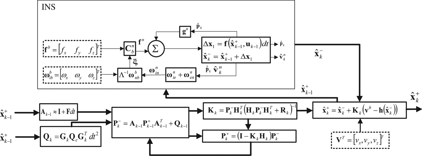
The block diagram of the conventional INS/DVL integrated navigation system is illustrated in Figure 1.

3. PROPOSED INTEGRATED NAVIGATION SYSTEM
In underwater vehicles, depth may be measured by a pressure sensor. In addition, in cruise conditions, the vehicle maintains a state of equilibrium, that is the vehicle's roll and pitch are small. Furthermore, the vertical component of the vehicle's velocity is usually small. This means that, in the proposed system, the required computations might be reduced to Two-Dimensional (2D) space. Hence, the transformation matrix  ${\bf C}_{b}^{n}$ would change to
 $${\bf C}_b^{\bf n} = \left[ {\matrix{ {cos\psi } & { - sin\psi } \cr {sin\psi } & {cos\psi } \cr } } \right]$$
In the proposed system, the state vector contains vehicle velocities in the north and east directions as  ${\bf v}^n = \left[ {\matrix{ {v_N} & {v_E} \cr } } \right]^T$, and the velocity measured by DVL
 ${\bf v}^b = \left[ {\matrix{ {v_x} & {v_y} \cr } } \right]^T$ is considered as an auxiliary measurement. After estimating the state vector, latitude and longitude are calculated through a Dead Reckoning (DR) algorithm. Assuming the vehicle has low velocity, the Coriolis effect
 $\lpar 2{\bi \omega}_{ie}^{n} + {\bi \omega}_{en}^{n}\rpar \times {\bf v}^{n}$ is always small and may be ignored and then the velocity equation can be rewritten as follows:
 $${\dot {\bf v}}^n = {\bf C}_b^n {\bf f}^{{\kern 1pt} b} + {\bf C}_b^n {\bf w}_a,{\bf f}^{{\kern 1pt} b} = \left[ {\matrix{ {f_{\bf x}} & {f_{\bf y}} \cr } } \right]^T$$
In the proposed system, the matrices Fk, Ak and Gk, and are obtained from Equation (27) as follows:
 $${\bf F}_k = {\bf 0},{\bf A}_k = {\bf I},{\bf G}_k = {\bf C}_b^n $$
where I and 0 are 2 × 2 identity and zero matrices. By assuming similar and independent accelerometers, Qk is computed as follows:
 $${\bf Q}_k \approx {\bf C}_b^n {\bf Q}_c{\rm (}{\bf C}_b^n {\rm )}^Tdt^2 = \sigma _a^2 {\bf I}dt^2$$
which shows that Qk is a diagonal matrix with the same elements at all time steps. Matrix H is computed from Equation (25) as follows:
 $${\bf H} = {\rm (}{\bf C}_b^n {\rm )}^{ - 1}$$
By assuming DVL measurements have independent and identically distributed noise in x and y directions, Equation (16) may be rewritten according to Equations (22) and (24) as:
 $${\bf P}_k^ - = {\bf P}_{k - 1}^ - - {\bf P}_{k - 1}^ - {\bf H}_{k - 1}^T {\rm (}{\bf H}_{k - 1}{\bf P}_{k - 1}^ - {\bf H}_{k - 1}^T + \sigma _v^2 {\bf I}{\rm )}^{ - 1}{\bf H}_{k - 1}{\bf P}_{k - 1}^ - + \sigma _a^2 {\bf I}dt^{\bf 2}$$
Since  ${\bf H}_{k}{\bf H}_{k}^{T} = {\bf I}$ and
 ${\bf P}_{k}^{-}$ is assumed to be a zero matrix at k = 0,
 ${\bf P}_{k}^{-}$ at k = 1 is given by the equation:
 $${\bf P}_1^ - = \sigma _a^2 {\bf I}dt^{\bf 2} = P_1{\bf I}$$
In other words,  ${\bf P}_{1}^{-}$ is a diagonal matrix with equal elements. Similarly, according to Equations (29) and (32),
 ${\bf P}_{2}^{-}$ may be given as follows:
 $$\matrix{ {{\bf P}_2^ - } \hfill & { = P_1{\bf I} - P_1{\bf H}_1^T {{\rm (}P_1{\bf H}_1{\bf H}_1^T {\bf I} + \sigma _v^2 {\bf I}{\rm )}}^{ - 1}{\bf H}_1P_1{\bf I} + \sigma _a^2 {\bf I}dt^{\bf 2}} \hfill \cr {} \hfill & { = P_1{\bf I} - \displaystyle{{P_1^2 } \over {P_1 + \sigma _v^2 }}{\bf I} + \sigma _a^2 {\bf I}dt^{\bf 2} = P_2{\bf I}} \hfill \cr } $$
The above equation shows that  ${\bf P}_{2}^{-}$ is also a diagonal matrix with equal elements. By generalising the above procedure, it can easily be shown that
 ${\bf P}_{k}^{-}$ is a diagonal matrix with the same elements at all time steps as
 ${\bf P}_{k}^{-} = P_{k}{\bf I}$. Generally, Equation (31) can be rewritten as:
 $$\matrix{ {{\bf P}_k^ - } \hfill & { = P_{k - 1}{\bf I} - P_{k - 1}{\bf H}_{k - 1}^T {{\rm (}P_{k - 1}{\bf H}_{k - 1}{\bf H}_{k - 1}^T {\bf I} + \sigma _v^2 {\bf I}{\rm )}}^{ - 1}{\bf H}_{k - 1}P_{k - 1}{\bf I} + \sigma _a^2 {\bf I}dt^{\bf 2}} \hfill \cr {} \hfill & { = \left( {\displaystyle{{\sigma _v^2 P_{{\rm k} - 1}} \over {P_{{\rm k} - 1} + \sigma _v^2 }} + \sigma _a^2 dt^{\bf 2}} \right){\bf I} = \left[ {\matrix{ {P_{\rm k}} & 0 \cr 0 & {P_{\rm k}} \cr } } \right] = P_k{\bf I}} \hfill \cr } $$
Although the model of the navigation problem is a time-varying model, it is possible to prove by mathematical induction that P k in Equation (34) is an asymptotic ascendant function which becomes equal to the constant value P:
 $$P = \displaystyle{{\sigma _a^2 dt^{\bf 2} + \sqrt {{\left( {\sigma _a^2 dt^{\bf 2}} \right)}^2 + 4\sigma _v^2 \sigma _a^2 dt^{\bf 2}} } \over 2}$$
If the vehicle is kept motionless for long enough before starting navigation, it can be assumed that P k equates to P from the first step time of navigation. In other words, from the instant of starting navigation, the constant value P can be used instead of P k. Therefore, Equation (22) may be changed to:
 $${\bf K}_k = \displaystyle{P \over {P + \sigma _v^2 }}{\bf C}_b^n $$
According to Equation (27),  $\hat{{\bf x}}_{k}^{-}$ is expressed as follows:
 $$\hat{{\bf x}}_k^ - = \hat{{\bf x}}_{k - 1}^ + + {\bf C}_b^n {\bf f}^{{\kern 1pt} b} dt$$
Using Equations (30), (36) and (37), Equation (23) may be expressed as:
 $$\eqalign{& d\hat{{\bf x}}_k^ + = \hat{{\bf x}}_k^ - + \displaystyle{P \over {P + \sigma _v^2 }}{\bf C}_b^n \left( {{\bf v}^b - {({\bf C}_b^n {\rm )}}^{ - 1}\hat{{\bf x}}_k^ - } \right) \cr & = \displaystyle{{\sigma _v^2 } \over {P + \sigma _v^2 }}\hat{{\bf x}}_{k - 1}^ + + {\bf C}_b^{\bf n} \left[ {\displaystyle{P \over {P + \sigma _v^2 }}{\bf v}^b + \displaystyle{{\sigma _v^2 dt} \over {P + \sigma _v^2 }}{\bf f}^{{\kern 1pt} b}} \right] \cr & = A\hat{{\bf x}}_{k - 1}^ + + {\bf C}_b^{\bf n} \left[ {B{\bf v}^b + C{\bf f}^{{\kern 1pt} b}} \right]} $$
The scalar coefficients A, B and C in Equation (38) can be computed off-line and it is not necessary to recalculate them during system operation.
After estimating the velocity components in the north and east directions, the latitude and longitude are computed by the following equations:
 $$L_k = L_{k - 1} + dt\displaystyle{{v_N} \over {R_N}},l_k = l_{k - 1} + dt\displaystyle{{v_EsecL_{k - 1}} \over {R_E}}$$
In Equation (38),  ${\bf C}_{b}^{{\bi n}}$ must be computed at each iteration. However, calculation of sine and cosine functions is not required for this purpose. The reason is that these functions may be expressed as follows:
 $$\left\{ {\matrix{ {\displaystyle{{d\left( {sin\psi } \right)} \over {dt}} = \dot \psi cos\psi } & {\buildrel {\dot \psi = \omega _{z,k}} \over \longrightarrow {\left( {sin\psi } \right)}_k = {\left( {sin\psi } \right)}_{k - 1} + \omega _{z,k}{\mkern 1mu} dt{\left( {cos\psi } \right)}_k} \cr {\displaystyle{{d\left( {cos\psi } \right)} \over {dt}} = - \dot \psi sin\psi } & {{\left( {cos\psi } \right)}_k = {\left( {cos\psi } \right)}_{k - 1} + \omega _{z,k}{\mkern 1mu} dt{\left( {sin\psi } \right)}_k{\rm }} \cr } } \right.$$
where ωz, k is the third component of the vehicle's angular velocity vector with respect to the navigation frame represented in the body frame  ${\bi \omega}_{nb}^{b}$, and is calculated as follows in the proposed system:
 $$\omega _{z,k} = r_k + \Omega sinL_k + v_{E,k}\displaystyle{{tanL_k} \over {R_E}}$$
where r k is the third component of the angular velocity vector  ${\bi \omega}_{ib}^{b}$ at time step k. So, Equation (40) may be expressed as follows:
 $$\left\{ {\matrix{ {C_{1,k} = {\left( {cos\psi } \right)}_k} & {\buildrel {\dot \psi = \omega _{z,k}} \over \longrightarrow C_{1,k} = C_{1,(k - 1)} + \omega _{z,k}dtC_{2,k}{\rm }} \cr {C_{2,k} = {\left( {sin\psi } \right)}_k} & {C_{2,k} = C_{2,(k - 1)} + \omega _{z,k}dtC_{1,k}} \cr } } \right.$$
Therefore, according to Equation (26), the transformation matrix at time step k is expressed as follows:
 $${\bf C}_{b,k}^n = \left[ {\matrix{ {C_{1,k}} & { - C_{2,k}} \cr {C_{2,k}} & {C_{1,k}} \cr } } \right]$$
From Equation (42) we see that the value of C 2, k has not yet been specified for computing C 1, k. To remedy this problem, the value C 2, (k−1) has been used instead of C 2, k. Accordingly, by using Equation (26) instead of Equation (42), we can reduce the computational load through omitting the calculation of sine and cosine functions.
4. EXPERIMENTAL RESULTS
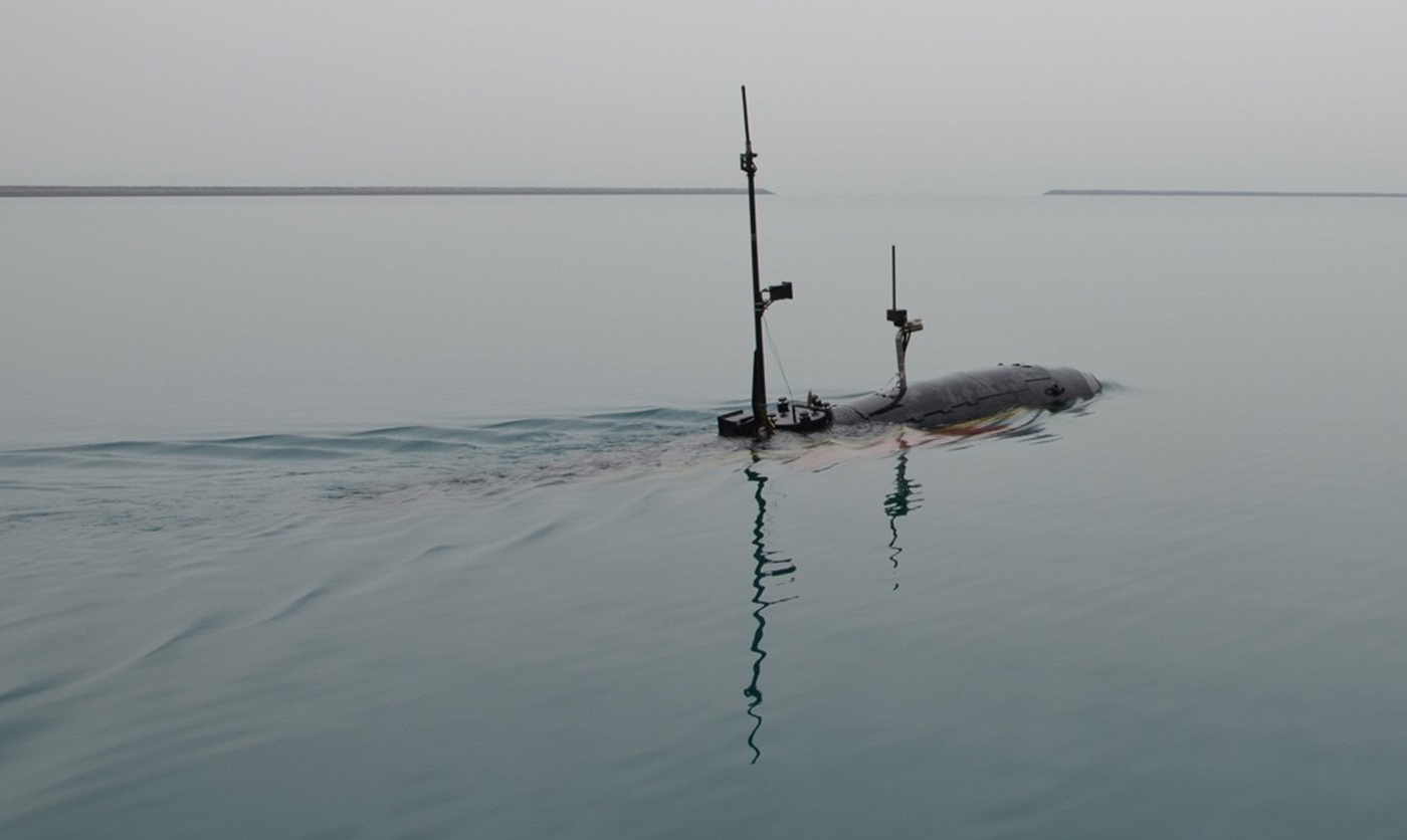
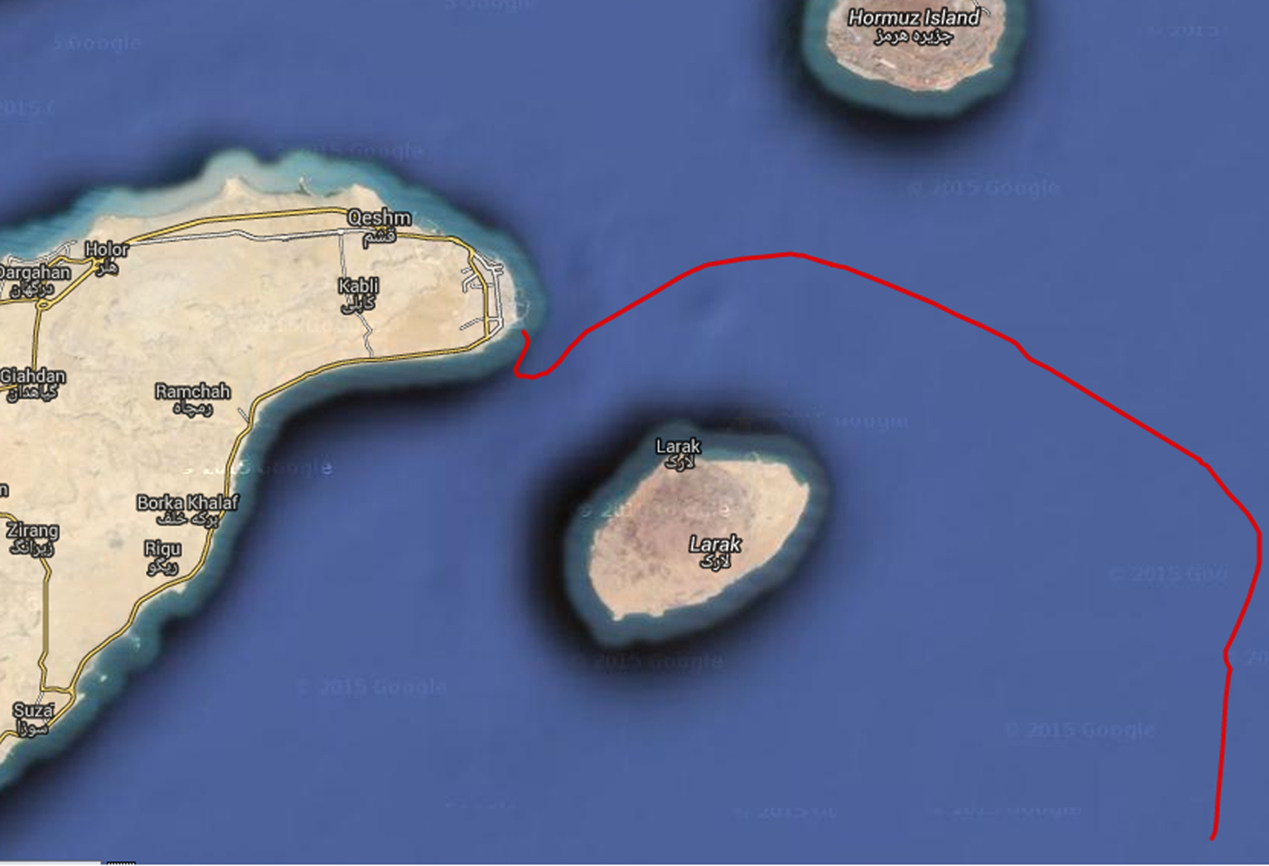
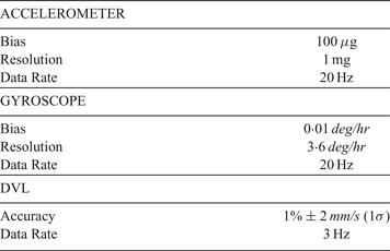
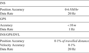
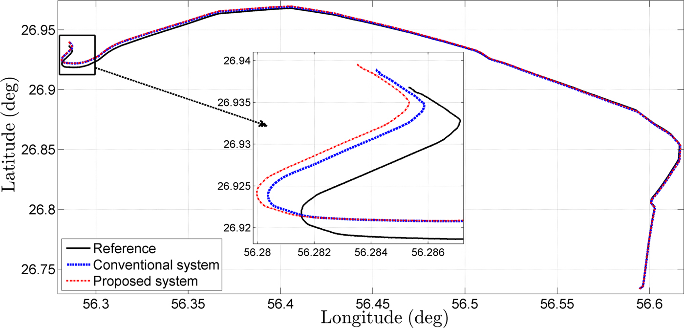
In this section, the performance of the proposed integrated navigation system is evaluated. For this purpose, a sea test was conducted using an AUV as shown in Figure 2. In this test, an Inertial Measurement Unit (IMU) and a DVL were utilised for navigation. A GPS and a high performance INS were used as the reference systems. In order to evaluate system accuracy, the position and velocity estimated by the proposed system are compared with those of a high performance INS/GPS/DVL integrated system. The technical specifications of the navigation and reference sensors are given in Tables 1 and 2, respectively. The trajectory travelled in the test is shown in Figure 3, in which the distance travelled and time are about 55·8 km and 4 hours, respectively.
The AUV used in the sea test.

Travelled trajectory in the sea test: In this test, approximately 55·8 km was travelled in 4 hours.

Technical specifications of the main instruments.

Technical specifications of the reference instruments.

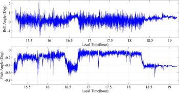
According to the dynamic equations given in Section 2.1, the depth variable is added in addition to the radius of the Earth. As submarines and AUVs usually move in depths less than 500 m, the depth is small compared with the radius of the Earth and drawing out the depth from the equations has no effect on the position accuracy. Moreover, as shown in Figure 4 the maximum values of roll and pitch angles of the AUV are 2 · 03° and 0 · 9° respectively and fluctuate around zero. Therefore, eliminating them from the navigation equations has minimal effect on the position accuracy.
Changes of roll and pitch during the test.

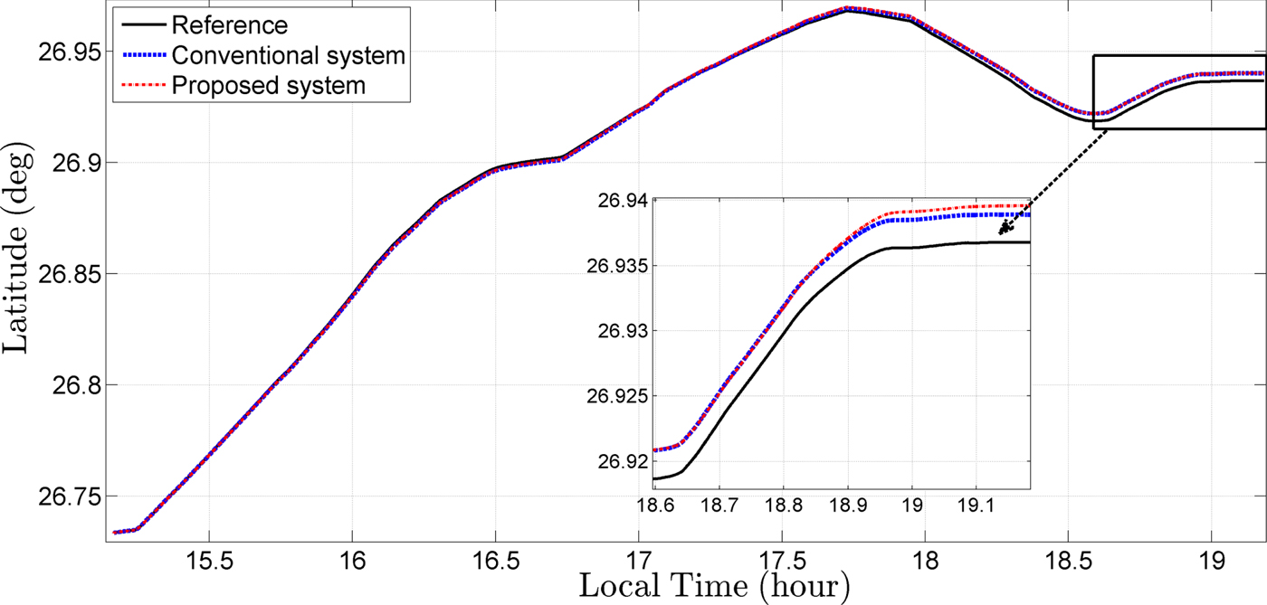
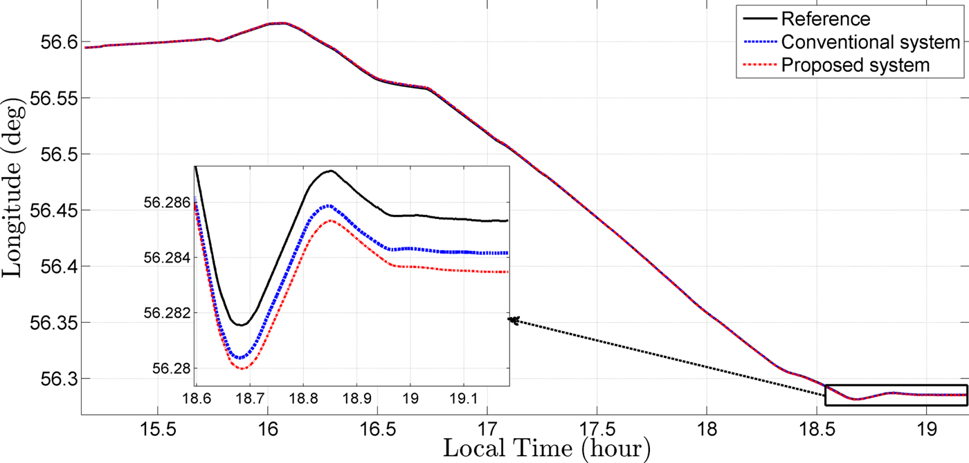
In Figures 5–7, the latitude, longitude and horizontal positions estimated by the proposed and conventional systems are shown. The position results imply that the accuracy of the proposed system is approximately equal to the conventional system. Note that the proposed method considerably reduces the computational burden.
Comparison of latitudes estimated by proposed, conventional and reference systems.

Comparison of longitudes estimated by proposed, conventional and reference systems.

Comparison of horizontal positions estimated by proposed, conventional and reference systems.

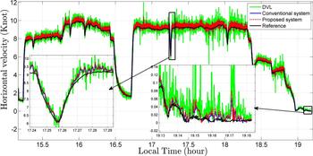
In order to validate the estimated velocity, the horizontal velocity is utilised and the curves of the horizontal velocity measured by the DVL and estimated by the navigation algorithms are compared with each other. The horizontal velocity in Knots is computed as follows:
 $$v_{h} = \left.\sqrt{v_{x}^{2} + v_{y}^{2}}\right/0{\cdot}5144$$
where v x and v y in m/s are the velocity components in the x and y directions. In Figure 8, the curves of the horizontal velocity estimated by the proposed and conventional systems are shown compared with the reference system.
Comparison of horizontal velocity estimated by the proposed, conventional and reference systems.

Although equations indicate that the Coriolis acceleration affects the speed of the AUV, the figures show that eliminating Coriolis acceleration does not have a great effect on the speed. This is due to the low speed of the AUV. The results of the estimated velocity also imply that the accuracy of the proposed system is identical to the conventional system.
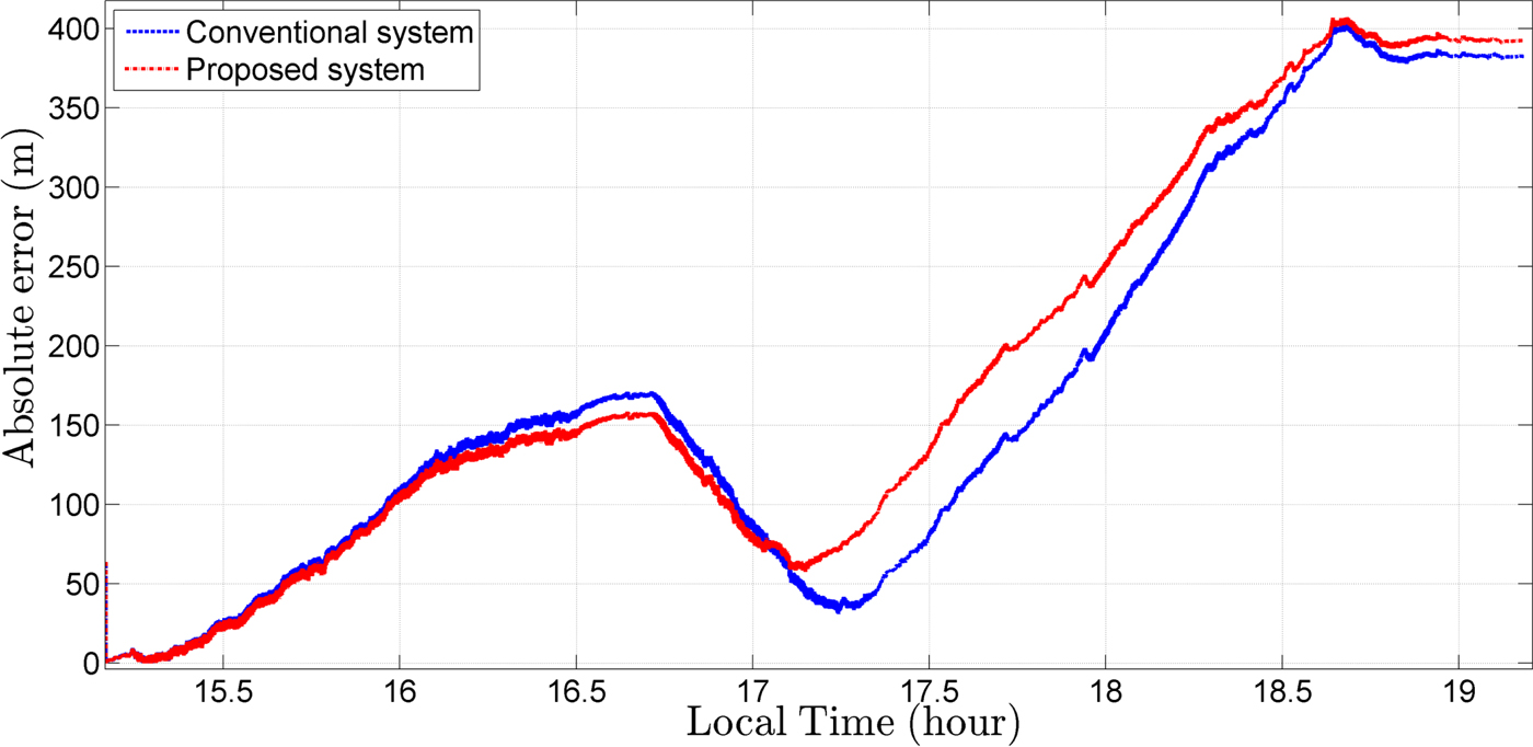
In order to evaluate the performance of the proposed system, the measure of absolute error of the estimated position can be used. The absolute error at time step k is denoted by:
 $$e_k = \left \vert {\displaystyle{{R\left( {L_{e,k} - L_{r,k}} \right)} \over {cos\alpha _k}}} \right \vert $$
where L e, k and L r, k are the estimated and the reference latitudes at time step k, respectively, and angle αk is obtained as follows (Forssell, Reference Forssell2008):
 $$\alpha _k = arctan\displaystyle{{l_{e,k} - l_{r,k}} \over {ln\left( {\displaystyle{{tan\left( {\displaystyle{{L_{e,k}} \over 2} - \displaystyle{\pi \over 4}} \right)} \over {tan\left( {\displaystyle{{L_{r,k}} \over 2} - \displaystyle{\pi \over 4}} \right)}}} \right)}}$$
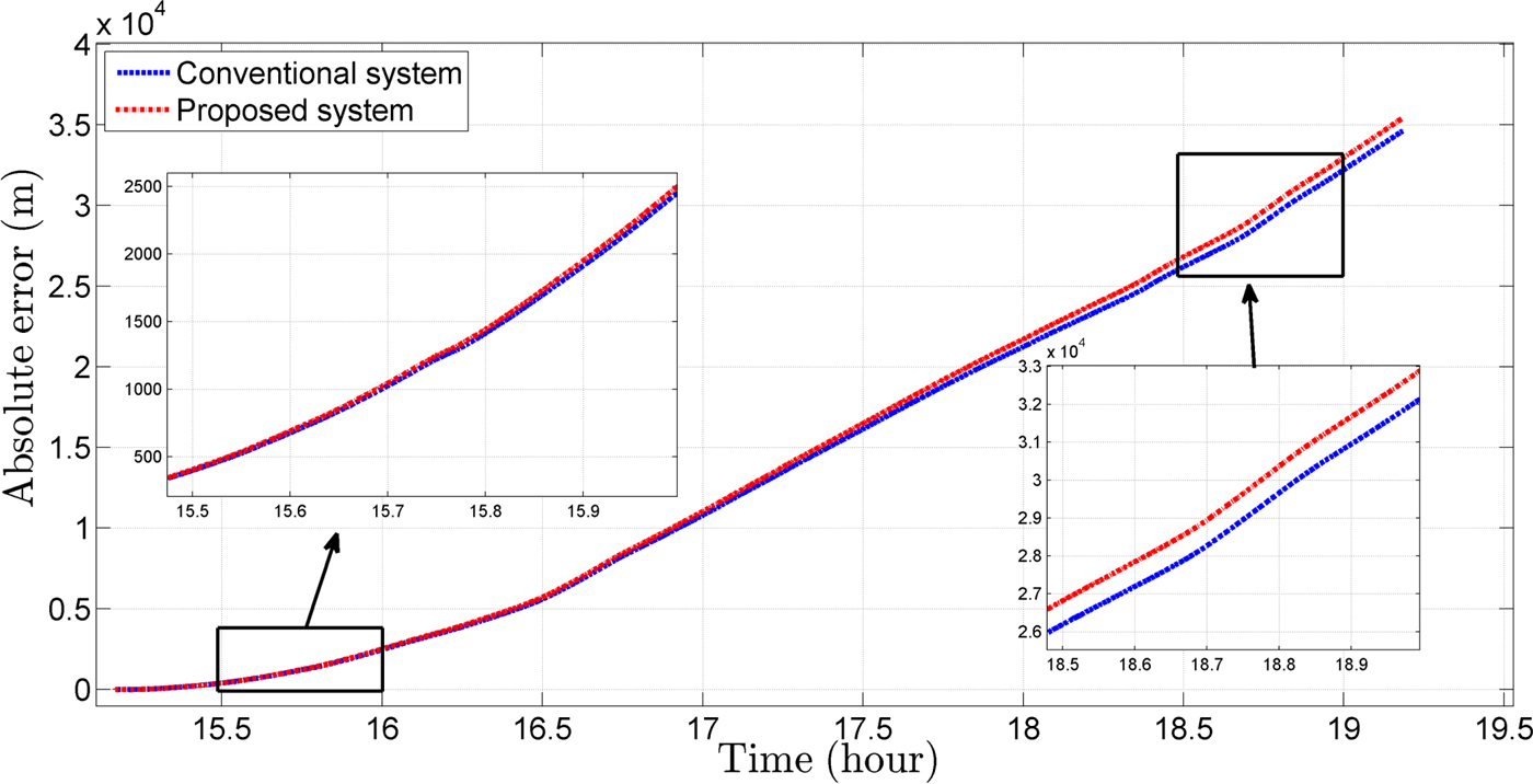
where l e, k and l r, k are the estimated and reference longitudes at time step k respectively. In Figure 9, curves of the absolute error of estimated position corresponding to the proposed and conventional systems are compared. It can be seen that the performances are close together. In pure inertial mode, Equation (38) changes to:
 $$\hat{{\bf x}}_k^ + = \hat{{\bf x}}_{k - 1}^ + + {\bf C}_b^{\bf n} {\bf f}^{{\kern 1pt} b}dt$$
In Figure 10, curves of the absolute error of the estimated position corresponding to the proposed and conventional systems in pure inertial mode are compared. Results show that, after about four hours, the proposed algorithm has increased the error to only 800 m, while the computational burden has significantly decreased compared with the conventional algorithm.
Comparison of the absolute error related to the position estimated by the proposed and conventional systems.

Comparison of the pure inertial absolute error related to the position estimated by the proposed and conventional systems.

In order to quantitatively compare the proposed system with a more conventional system, Root Mean Square Error (RMSE) is used for position and velocity estimations defined by the following equations:
 $$Position \,RMSE = sqrt\left( {mean(e_k^2 )} \right)$$
 $$Relative \, RMSE = \displaystyle{{RMSE} \over {Travelled \, Distance}} \times 100$$
 $$Velocity\, RMSE = sqrt\left( {mean\left( {{\left( {v_{h,r} - v_{h,e}} \right)}^2} \right)} \right)$$
where v h, r and v h, e are the reference and the estimated horizontal velocity. In the performed test, the RMSE values of position estimated by the proposed and conventional systems are 223 m and 211 m, respectively, and their relative values are 0·4% and 0·38%, respectively. The RMSE of velocity estimated by the proposed and conventional systems are 0·214 Knots and 0·192 Knots, respectively.
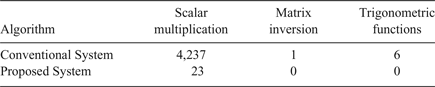
The point to be focused on here is that the superiority of the proposed system is in having a low computational load. In order to evaluate the computational complexity, the number of operations including the scalar multiplication, matrix inversion and trigonometric functions are compared in both the proposed and conventional systems. The conventional system needs 4,237 scalar multiplications, one matrix inversion and six trigonometric calculations while in the proposed system only 23 scalar multiplications are executed.
In order to compare the computational load of the algorithms, the conventional and proposed algorithms were implemented on an Intel Core2Duo CPU (E7300, 2·66GHz). It can do 2·9 Giga Floating point Operations Per Second (2·9 GFLOPS). Experimental results show that each time step of the conventional algorithm takes 0·2 ms on this CPU, while the proposed algorithm takes 0·015 ms. In other words, the conventional algorithm requires an execution time 13 times longer than that of proposed algorithm to achieve the same precision. This shows a significant decrease in the computational load.
A summary of the field results and a comparison of the number of computational operations are given in Tables 3 and 4.
Summary of the performance evaluation for the proposed and conventional systems in the field tests.

Comparison of the computational operations in the proposed and the conventional systems.

5. CONCLUSION
The objective of this study was a reduction of the computational burden in a conventional underwater integrated navigation system. The conventional systems consist of a 3D INS and a 3D DVL, and in these systems, data incorporation is performed by a Kalman filter, that is by a 3D form of computations. In the proposed system, assuming only small variations of roll and pitch angles and depth being available through a pressure sensor, computations were performed in a 2D form. The nonlinear model of the system was also simplified to a linear model due to the low speed of the test vehicle. Furthermore, a low complexity KF algorithm was proposed according to the simplifications of the state covariance matrix. In order to evaluate the performance of the proposed system, a sea test was conducted. Results demonstrate that the proposed system can have a performance similar to a conventional system, while considerably reducing the computational burden.