2. PROBE AND ADJUST

An individual probes by just trying an act at random, and then adjusts by:

1. (i) adopting the new act if it has a higher payoff than the old one

2. (ii) going back to the old act if the new one got a lower payoff or

3. (iii) flipping a coin to decide if they are equal.

In a repeated choice situation an individual probes and adjusts with small probability, e, and just chooses the same as last time with probability (1-e). We start the process by just choosing at random.

We illustrate by applying probe and adjust dynamics to a one-person decision problem: a bandit problem. You have two slot machines, R; L, each of which pays off with a different unknown probability. (Trials are independent and identically distributed, and are independent between machines.) Can you learn to play the optimal machine?

In probe-and-adjust learning, nothing happens except when there is a probe. We can analyze it by looking only at pre-probe and post-probe states. This embedded sequence is a Markov chain. We can analyze as follows. Suppose bandit L pays off with probability p and bandit R pays off with probability q. The state of playing bandit R transitions to that of playing bandit L with probability:

Likewise, L transitions to R with probability:

The matrix of transition probabilities is shown in Table 1. Obviously, this is an ergodic Markov chain. That is to say no matter where you start, you get to an invariant probability distribution. In this case, you get there immediately. It is:

Table 1.

The Matrix of Transition Probabilities

If, for instance, R pays off 90% of the time and L 50%, probe and adjust plays R 70% of the time + some correction for probes, depending on the probe probability. If probes are infrequent, this is close to the actual play frequency. Probe and adjust favors the higher paying bandit, but does not learn optimal play.

In the special case where p + q = 1, the invariant distribution of the embedded pre-probe, post-probe Markov chain is:

With infrequent probes, a machine is played with the probability close to its payoff. This is some version of what psychologists call ‘probability matching’. It has been frequently observed in human learning experiments, and discussions of its robustness have generated a large and sometimes contentious literature in psychology and economics (Vulkan Reference Vulkan2000).

3. SIGNALING GAMES

Sender–Receiver signaling games were first introduced by David Lewis in Convention (Reference Lewis1969). There are two players, a sender and a receiver. The sender observes a situation, which nature chooses at random. She chooses a signal, conditional on the situation observed. The receiver observes the signal, and chooses an act, conditional on the signal observed. Payoffs for sender and receiver are determined by the combination of signal and situation. Signals are cost-free and sender and receiver have pure common interest. In the simplest case, there is an act that is ‘right’ for each situation in that if that act is done in that situation both sender and receiver get a payoff of 1, and otherwise they get a payoff of 0. For simplicity, we can index that situations and acts such that the joint payoff on 1 occurs just in case act A_i is done in situation S_i. (Situations are also called ‘states’, but we use ‘situation’ where there could be confusion with the state of a Markov chain.)

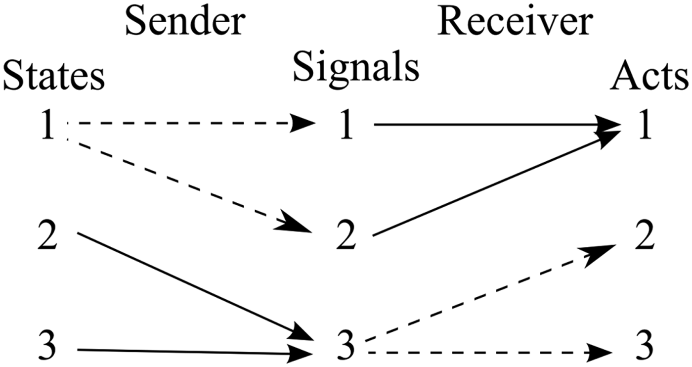
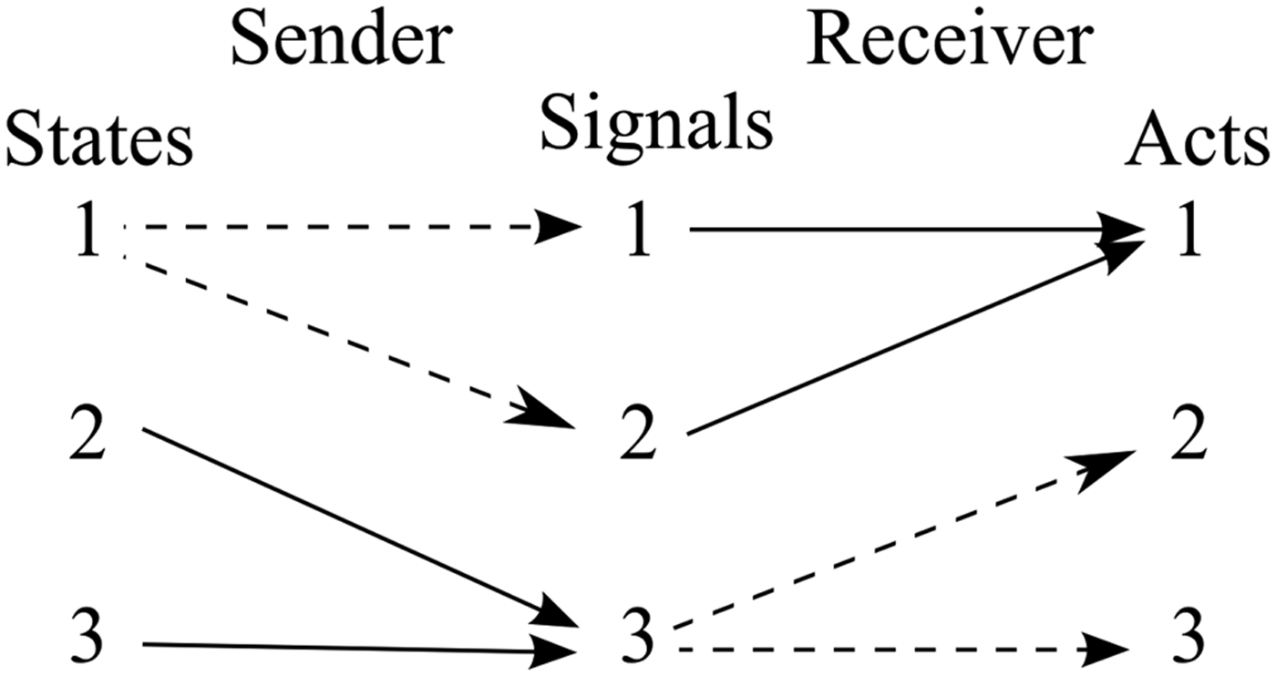
Lewis calls an equilibrium in which players always receive a payoff of 1 a signaling system equilibrium. There are other equilibria. If the sender sends signals with probabilities independent of the situation and the receiver chooses acts independent of the signals, we have a total pooling equilibrium. All the situations are pooled, in that the signal sent carries no information about the situation. It is an equilibrium in that neither sender nor receiver can improve her payoff by changing her behavior. If there are more than two situations, there may be partial pooling equilibria in which some but not all states are pooled. For example, suppose there are three situations, three signals and three acts, and that the sender sends:

and the receiver does:

This is a partial pooling equilibrium in which situations 1 and 2 are pooled. See Figure 1. Many generalizations and variations are of interest, but here we concentrate on the basic signaling game.

Fig. 1.

A Partial Pooling Equilibrium

4. LEARNING TO SIGNAL WITH PROBE AND ADJUST: THE SIMPLEST CASE

There are two situations, two signals and two acts. Nature flips a fair coin to choose a situation {1 or 2}, the sender observes the situation and chooses a signal {A or B} and the receiver observes the signal and chooses one of two acts {1 or 2}.

Consider probe and adjust learning applied to this signaling game. We assume that each sender treats each situation as a separate choice stimulus. Each receiver treats each signal received as a separate choice stimulus. In order to apply probe and adjust, individuals must remember not just what happened last time, but what happened last time for each stimulus. So the sender remembers what he did the last time he was confronted with situation 1 and the payoff he received and likewise for situation 2. The receiver remembers what he did last time and the payoff received when observing signal 1 and likewise for signal 2. Memory requirements are still quite modest.

Most of the time agents just repeat what they did last time for the same stimulus. Every once in a while an agent probes and adjusts. We assume here that only one agent probes and adjusts at a time. The other agent keeps doing the same thing during the probe-and-adjust process. Now we can again find an embedded Markov chain that consists of pre- and post-probe-and-adjust transitions. Here the state of the system of both players consists of a pair: a map from situations to signals for the sender and a map from signals to acts for the receiver. This is just the memory of what they did last given the respective stimuli. (Note that this system state enables us to calculate the payoffs that they got last time they did something.)

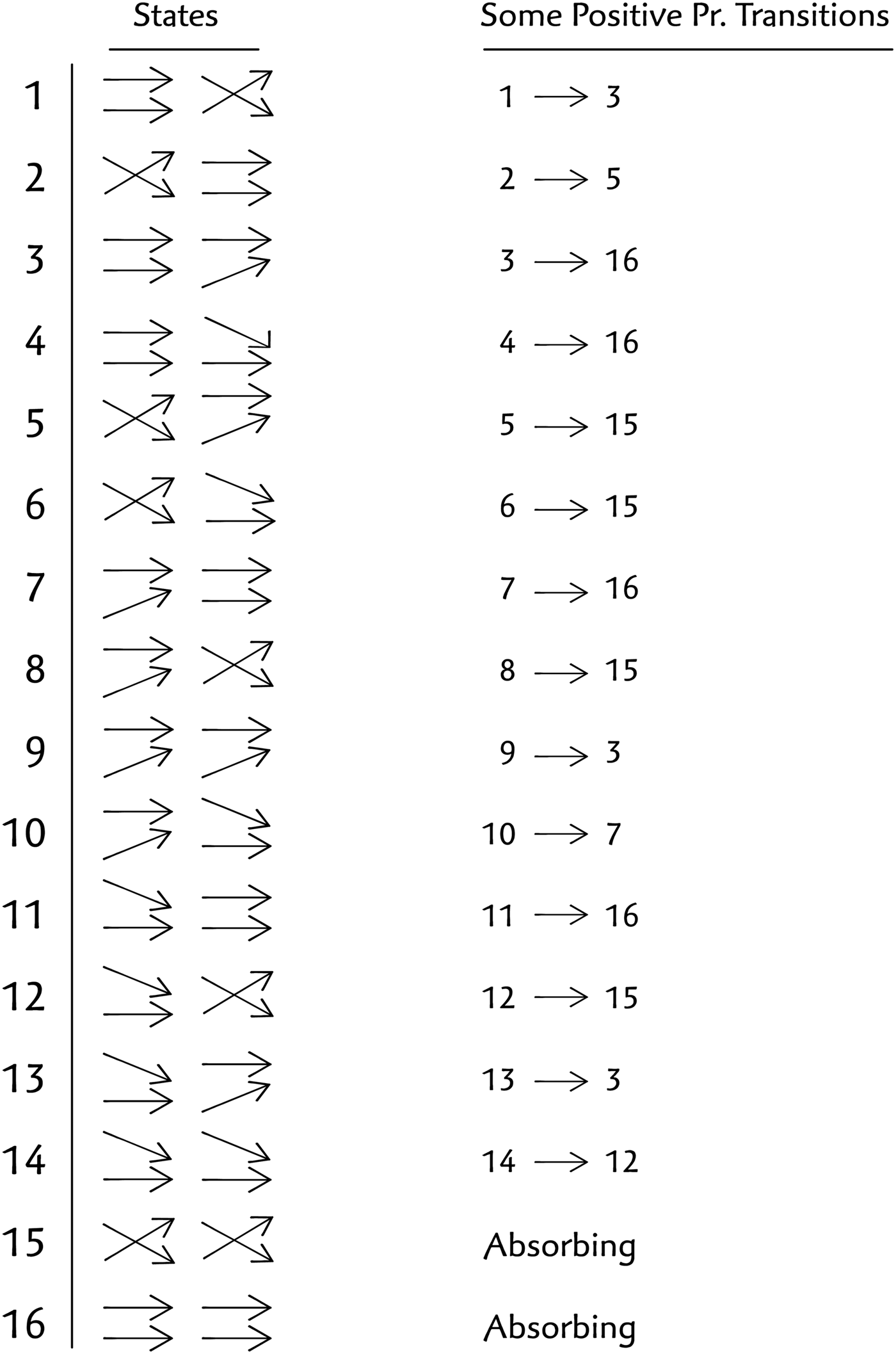
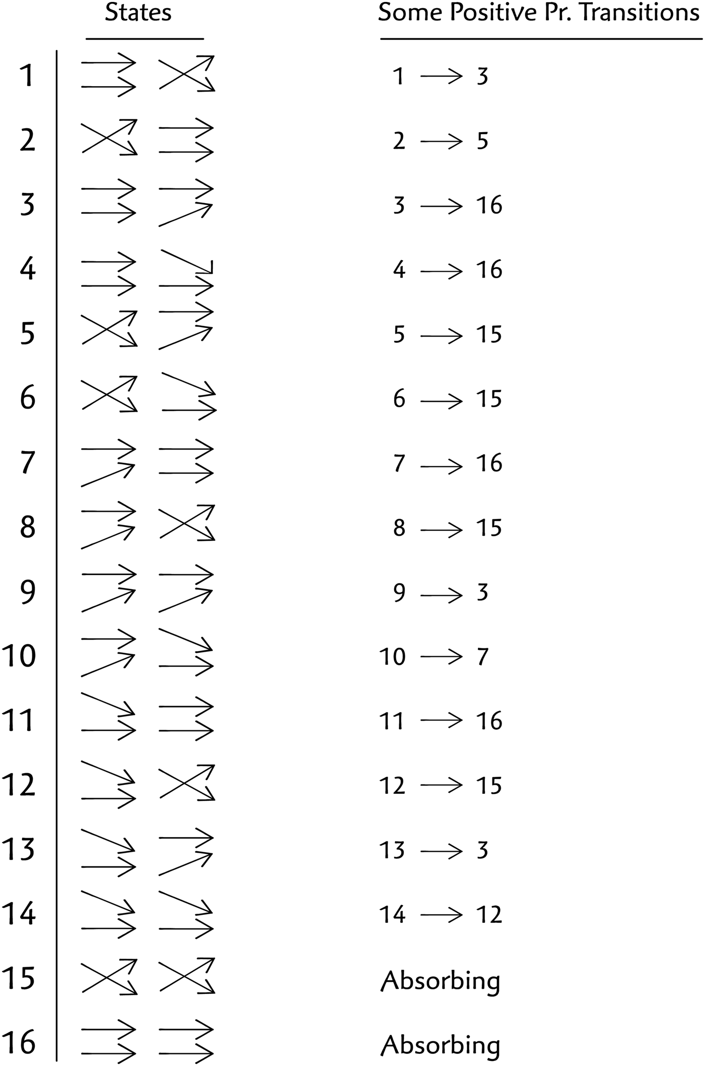
There are four possible sender configurations and four receiver configurations, so there are sixteen possible states of the system as shown in Figure 2.

Fig. 2.

States and Transitions 2 situations / 2 signals / 2 acts

The transition probabilities are calculated as follows. Nature chooses the sender or receiver to probe by flipping a fair coin. Nature chooses a situation by flipping a fair coin. If sender is chosen sender probes a new signal for the situation chosen. If receiver is chosen, sender sends the old signal for the situation and receiver probes a new act for the signal. Then if the probe gave a higher payoff the new configuration is adopted; if it gave the same payoff the new configuration is adopted with probability ½; if it gave a lesser payoff the system remains in the original state.

This Markov chain, unlike that for the bandit problem, is not ergodic. States 15 and 16, which correspond to the two signaling systems, are absorbing states. Once entered the Markov chain will not leave them. Any probe will get a smaller payoff, and the agents will adjust back to the original state. Furthermore, as we will see, they are the only absorbing states. If the agents enter one of these states, we will say that they have learned to signal. This means that they will continue in the signaling system except for occasional fruitless probes that will lead them to return to it. Figure 2 shows some (not all) positive probability transitions between states.

States 15 and 16 are signaling systems. States 3, 4, 5, 6, 7, 8, 11 and 12 can move to a signaling system with one probe. Each of the other states can move to one of these (States 3, 4, 5, 6, 7, 8, 11 or 12) with one probe. Thus, from any state there is a (short) positive probability path to a signaling system. It follows that with probability one, probe and adjust learns to signal. We will investigate how this logic generalizes.

5. PROBE AND ADJUST: N EQUIPROBABLE SITUATIONS, N SIGNALS, N ACTS

As in the simplest case, when we consider transitions between pre-probe-adjust states and post-probe-adjust states, we have an embedded Markov chain. The state of the system for this chain consists of a record of what was done last in each situation by the sender and last for each signal by the receiver. It is thus a pair of sender and receiver functions, <f, g>. These are functions since each only remembers what she last did in the each decision situation. These need not be one to one, as the sender may have sent the same signals in multiple situations and the receiver may have done the same act on receiving multiple signals.

The analysis of the simplest game generalizes. Specifically:

1. (1) Signaling systems are absorbing states of the Markov chain.

2. (2) Signaling systems are the unique absorbing states.

3. (3) From any state, there is a positive probability path to a signaling system.

For (1):

For (2):

For (3):

The Markov chain always reaches an absorbing state.

One might ask how individuals begin to learn. In defining the states of the Markov chain, we assumed there was always a history. Shouldn't we redo the Markov analysis allowing partial functions for sender and receiver histories, and allowing random choices when a new stimulus with no prior history is reached? This doesn't really change anything. We treat undefined functions just like failures for the purposes of probe and adjust. Then the foregoing algorithm works the same way. There is still a positive probability path from any state to a signaling system. Agents always learn to signal perfectly. Here probe and adjust learning always achieves optimal signaling.

6. EXTRA SIGNALS: N EQUIPROBABLE SITUATIONS, M SIGNALS, N ACTS (M > N)

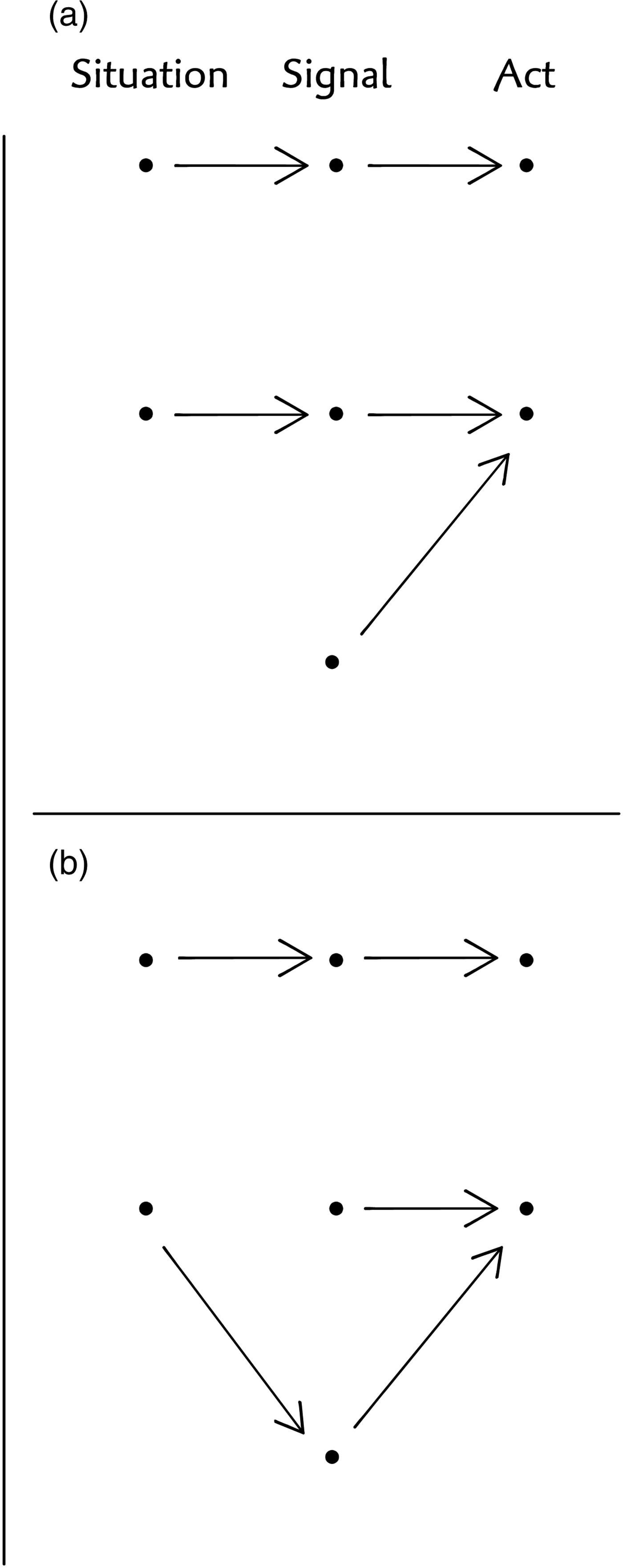
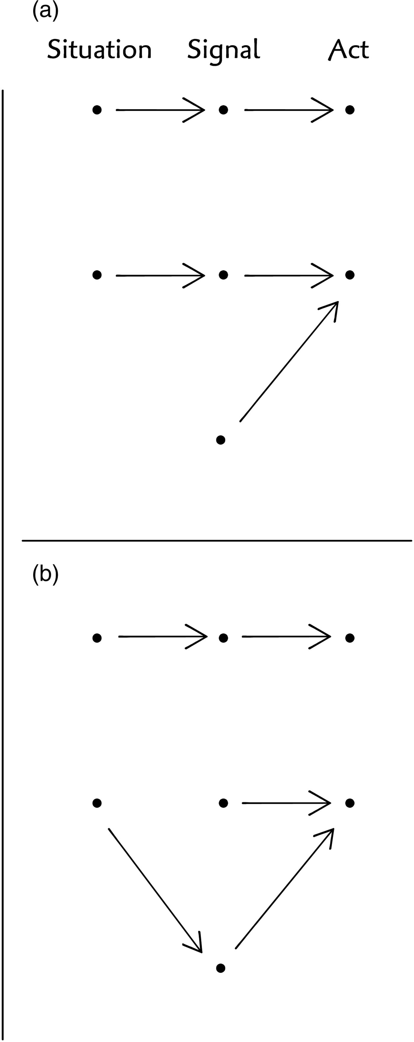
If we have excess signals, the picture changes. The embedded Markov chain generated by probe and adjust no longer has any absorbing states. Efficient states – those where g(f(s)) is the identity – of the system consist of an N by N by N signaling system together with M-N signals that are not sent. These signals are mapped onto some acts by the receiver's memory. Suppose some unused signal is mapped onto A_i. If the sender probes by sending the unused signal instead of the signal he usually sends in S_i, then the probe does not change his payoff. Then with some probability he adjusts by retaining the new signal in place of the old. (A receiver cannot probe changing an unused signal, since a receiver is not probing a new function, g, but only what to do if confronted with a signal. If a signal is unused, a receiver is not confronted with it.)

For example, in Figure 3, probe and adjust can lead from state A to B and state B to A but not outside the set. Check all other possible probes. They don't lead anywhere. This is an absorbing set (an ergodic set). Within the set, signals 2 and 3 can be thought of as sequential synonyms. One is used for situation 2 for a while and then the other is. After the system has been absorbed into this set, there is a long-term invariant distribution within the set. Signals 2 and 3 are each used half the time for situation 2. There are lots of such ergodic efficient sets.

Fig. 3.

An absorbing set with sequential synonyms.

It is still true that from any state there is a positive probability path to an efficient ergodic set. The same algorithm as before works for the same reasons. Applying the algorithm until one runs out of states gives a path to a member of an efficient ergodic set. Probe and adjust still learns to signal with probability one.

7. TOO FEW SIGNALS: N EQUIPROBABLE SITUATIONS, M SIGNALS, N ACTS (M < N)

In this case, partial pooling is the best that can be done. There are not enough signals for a signaling system to map each state onto the appropriate act. The best average payoff achievable is (M/N), gotten when for each signal, s, g(s) in f⁻¹(s). The structure of these efficient signaling equilibria is investigated in Donaldson et al. (Reference Donaldson, Lachmann and Bergstrom2007). Consider the case of M = 2, N = 3. In the efficient equilibria the sender pools two situations. There are three choices of situations to pool. For each, there is a choice of which signal to assign to the pooled states. So there are six sender's strategies that are components of efficient equilibria. On the receiver's side, for such a sender's strategy there are two situations pooled, so it makes no payoff difference if the receiver does the right act for one or for the other. Thus two receiver's strategies pair with each of the six sender's strategies to make twelve optimal equilibria. This is shown in Figure 4.

Fig. 4.

12 equilibria. From Donaldson, et. al.

Probe and adjust can move from one of these equilibria to another. Adopting the notation of the figure (s for situation, t for signal, a for act), suppose that we start at:

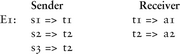
The sender pools situations 2 and 3. Suppose nature chooses s3, sender sends t2 and receiver probes a3. Receiver gets a payoff of 1, which, at worst, ties previous payoff for doing a2 upon seeing t2. So with positive probability receiver switches, taking us to:

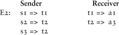
This step is reversible; a probe can take us back to E1.

Now the receiver never does a2, so it doesn't matter if the sender pools s2 with s1 or with s3. Suppose nature chooses s2, and sender probes t1. This leads to 0 payoff, which matches sender's previous payoff in s2, so with positive probability sender switches, leading to:

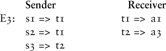
(This step is also reversible.) But now sender is pooling s1 and s2, so by the same logic as before a receiver's probe can lead to:

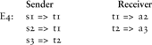
And now receiver never does a1, in turn setting up a sender's probe that can lead to:

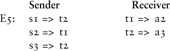
The process continues through a cycle of the twelve efficient equilibria. All these efficient states form one ergodic set. As probe and adjust moves through this set, signals shift their meaning. To show that there is a positive probability path from any state to a state in the efficient ergodic set, use the same algorithm as before. When you run out of signals you are done. Probe and adjust leads to efficient signaling.

8. SITUATIONS WITH UNEQUAL PROBABILITIES

So far, states have been supposed to have equal probabilities. There is to date no rigorous analysis of reinforcement learning in situations with unequal probabilities. But preliminary analyses and computer simulations point to the conclusion that in this case reinforcement learning can lead to total pooling equilibria. Consider the case of two situations, signals and acts in which situation 1 is highly probable. Then a total pooling equilibrium in which the receiver just does act 1 and ignores the signals, and the sender ignores the state and always sends the same signal, is not so implausible. Players usually get paid off without bothering much with signaling. Simulations show reinforcement learning sometimes converging to a signaling system, sometimes to total pooling.

How does Probe and Adjust do with unequal probabilities? Notice that none of our foregoing analysis made use of the assumption of equal situation probabilities. We only need that situation probabilities are all positive in order to construct the positive probability paths leading to absorbing sets or states. Probe and adjust dynamics learns to signal perfectly in N situation, M signal, N act signaling games when there are enough signals (M > = N).

In the case where there are too few signals, M < N, efficiency imposes an extra requirement. Since there are not enough signals, states have to be pooled. In an efficient configuration, the highest probability states must be serviced in a way that maximizes expected payoff.

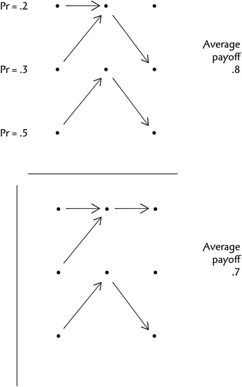
For example, suppose that M = 2, N = 3, and states 1, 2, 3 have probabilities .2, .3, .5 respectively. One efficient configuration will have the sender map states 1 and 2 onto one signal that the receiver maps to state 2, and have the sender map state 3 onto the other signal, which the receiver maps to act 3. Then the average payoff is .8. But probe and adjust may lead from this efficient state to an inefficient one, as shown in Figure 5.

Fig. 5.

Efficient and inefficient members of the ergodic set.

In situation 1 sender sends signal 1 and receiver probes act 1. This gets a payoff of 1, which matches the receiver's memory of a payoff of 1 for doing act 2 on receiving signal 1. The tie is broken by a coin flip, so with some probability, receiver stays with the probe. The receiver has no memory of the frequencies of payoffs – only of the magnitude of the last payoff. Probe and adjust can move around the whole ergodic set of the preceding section. This weakness of probe and adjust here is just the other side of the coin from its strength. Absorption to an ergodic set is what allows it to so reliably learn to signal with situations of unequal probabilities.

We do not always learn to signal efficiently, but we always learn to signal. That is, of course, with the proviso that ‘learning to signal’ always includes occasional probes away from a signaling system.

9. PAYOFF-DEPENDENT PROBE PROBABILITIES

Probe and adjust has a constant probability of probing. A natural modification makes the probability of probes payoff-dependent: the worse the payoff, the more likely a probe. One special case deserves note. Suppose that our trial and error learner has an idea of an optimal payoff. Then she may not probe at all if the last payoff was optimal.

In our signaling games, suppose a player does not probe at all if the last trial was a success, but probes with some probability (greater than 0 and less than 1) if the last trial was a failure. (Compare Barrett and Zollman (Reference Barrett and Zollman2009).) Then the positive results of the preceding discussion are retained, but residual probing is eliminated. (And it is no longer necessary to include the assumption that there are no simultaneous probes.) These agents always find a signaling system by trial and error, and then stick to it.

10. RELATED WORK

The need for low rationality game theory is emphasized in Roth and Erev (Reference Roth and Erev1995), Erev and Roth (Reference Erev and Roth1998), Fudenberg and Levine (1998), and Young (Reference Young2004, Reference Young2009). Probe and adjust can be seen as a version of the one-element stimulus sampling model of Estes (Reference Estes1950). Estes learning theory was applied to game theory in the pioneering work of Suppes and Atkinson (Reference Suppes and Atkinson1960). There are more complicated versions of probe and adjust type learning, with more memory and payoff dependent probes, which perform well very generally (Marden et al. Reference Marden, Young, Arslan and Shamma2009; Young Reference Young2009).

Equilibrium structure of signaling games with many or few signals is analyzed in Donaldson et al. (Reference Donaldson, Lachmann and Bergstrom2007). Two-population replicator dynamics of a two situation, two signal, two act signaling game where the situations have unequal probabilities is analyzed, with and without mutation, in Hofbauer and Huttegger (Reference Hofbauer and Huttegger2008).