1 Introduction
Particle-laden fluid flows arise in a diverse range of industrial and geophysical problems including slurry pipelines for transporting oil or coal, mining and milling operations, stimulation of unconventional geo-energy resources (e.g. use of proppants in hydraulic fracturing), fluidized beds, abrasive water jet machining, debris flows, landslides and sediment transport. In some of these flows, solid-phase impacts may deform or erode a solid surface, like a pipe wall, a rock surface or a stream bed (e.g. Clark (Reference Clark1991), Sklar & Dietrich (Reference Sklar and Dietrich2001)). The wear can lead to failure of equipment, leaks in pipelines or changes in stream beds and rock masses. Within these applications, there is often a need to predict the erosion or wear rate for a given flow, where the erosion rate is typically defined in terms of the mass or volume change in a given time or for a given mass of particle moving along or towards a surface.
Some erosion models are based on the plasticity theory that predicts the size of a crater formed from an individual particle impact, either normal or oblique (e.g. Finnie (Reference Finnie1960, Reference Finnie1972), Bitter (Reference Bitter1963a ,Reference Bitter b ), Hutchings (Reference Hutchings1981)). In these plasticity studies, the volume of material removed due to particle impacts depends on the impact angle and the kinetic energy of the impacting particle and on the material properties. Other factors, such as the relative hardness of the surface to the impactor, surface treatments or work hardening effects, also affect the erosion process (Bitter Reference Bitter1963a ,Reference Bitter b ). Models have been developed to predict the erosion rate of a surface given the flow characteristics by using plasticity analysis to compute the volume removed during a single impact and then multiplying it by a representative number of collisions in a given time and area (Sklar & Dietrich Reference Sklar and Dietrich2004; Lamb, Dietrich & Sklar Reference Lamb, Dietrich and Sklar2008; Chatanantavet & Parker Reference Chatanantavet and Parker2009). The representative number of collisions depends on characteristics of the flow, such as the flow Reynolds numbers, shear stress along the bed, particle concentration, grain size distribution and the flow rate. Other models use an empirical approach to relate the mass or volume loss to the velocity of solid particles, mean particle diameter, impact angle and the hardness of materials. As described in Desale, Gandhi & Jain (Reference Desale, Gandhi and Jain2011), the parameters used in erosion correlations vary widely because of the range of materials, fluids properties and flow conditions under which the correlations have been developed. The recent review by Parsi et al. (Reference Parsi, Najmi, Najafifard, Hassani, McLaury and Shirazi2014) on slurry erosion in oil and gas wells and pipelines lists approximately 30 different parameters that have been used to predict the material loss for a wide range of impact conditions.
The focus of the current work is to measure the coefficient of restitution and the crater dimensions for normal particle–wall impacts over a range of impact speeds, different interstitial fluids and impacted metals. In addition, the paper develops models that are compared with the measurements to predict the size of the craters and the rebound speeds. In debris or slurry flows, the speeds of the particles can be of the order of centimetres to several metres per second. For metal surfaces, used in this study, these speeds correspond to impacts within the elastic–plastic range, which is more complex to model than the pure elastic or pure plastic collisions because of the uncertainty regarding the relationship between force and material deformation (Thornton Reference Thornton1997; Jackson, Green & Marghitu Reference Jackson, Green and Marghitu2010; Wang, Geubelle & Lambros Reference Wang, Geubelle and Lambros2013; Burgoyne & Daraio Reference Burgoyne and Daraio2014). The experiments conducted in this work fall in the elastic and elastic–plastic ranges. The particle Reynolds numbers vary from 5 to 2500, where
 $Re=2R\unicode[STIX]{x1D70C}_{f}u_{o}/\unicode[STIX]{x1D707}$
; R is the particle radius,
 $\unicode[STIX]{x1D70C}_{f}$
and
 $\unicode[STIX]{x1D707}$
are the density and dynamic viscosity of the fluid and
 $u_{o}$
is the particle velocity just before the impact. The Stokes numbers vary from 2 to
 $3\times 10^{5}$
, where
 $St=2R\unicode[STIX]{x1D70C}u_{o}/(9\unicode[STIX]{x1D707})$
and
 $\unicode[STIX]{x1D70C}$
is the particle density. In this range, both viscous and inertial effects are important in considering the approach and rebound of the particle. These impact conditions were also considered by Ruiz-Angulo & Hunt (Reference Ruiz-Angulo and Hunt2010); different from this prior study, however, the current work includes measurements of the crater dimensions. Also, an analytical relation is developed for the coefficient of restitution in terms of the properties of the fluid and solid, which agrees well with the experimental data acquired in this study. The crater dimensions are used to validate the analytical relations developed here based on elastic and plastic theories and energy balance considerations.
As background, the next section describes the impact and rebound process for elastic, plastic and mixed elastic–plastic collisions, and the effect of a viscous fluid on the collision process. Additional details on the analysis of elastic–plastic deformations are given in appendix A.
2 Theory
2.1 Models of a particle impacting a surface
2.1.1 Pure elastic collisions
The analysis based on the Hertz (Reference Hertz1881) theory of elasticity is briefly summarized here. Consider an elastic sphere with modulus of elasticity
 $E_{1}$
, Poisson’s ratio
 $\unicode[STIX]{x1D708}_{1}$
and radius
 $R$
impacting normal to a smooth elastic half-plane with modulus of elasticity
 $E_{2}$
and Poisson’s ratio
 $\unicode[STIX]{x1D708}_{2}$
. From elasticity theory, the elastic contact radius,
 $a_{e}$
, and the indentation depth,
 $\unicode[STIX]{x1D6FF}_{e}$
, are
 $$\begin{eqnarray}\displaystyle & \displaystyle a_{e}=\frac{\unicode[STIX]{x03C0}}{2}\frac{P_{o}}{E^{\ast }}R, & \displaystyle\end{eqnarray}$$
 $$\begin{eqnarray}\displaystyle & \displaystyle \unicode[STIX]{x1D6FF}_{e}=\frac{\unicode[STIX]{x03C0}}{2}\frac{P_{o}}{E^{\ast }}a_{e}, & \displaystyle\end{eqnarray}$$
 $E^{\ast }=[(1-\unicode[STIX]{x1D708}_{1}^{2})/E_{1}+(1-\unicode[STIX]{x1D708}_{2}^{2})/E_{2}]^{-1}$
, and
 $P_{o}$
is the maximum stress at the contact. The normal stress distribution during contact with respect to the radial distance from the crater centre
 $r$
is
 $P(r)=P_{o}(1-r^{2}/a_{e}^{2})^{1/2}$
, from which the mean elastic force acting during the deformation,
 $F_{e}$
, is calculated as
 $F_{e}=2/3\unicode[STIX]{x03C0}a_{e}^{2}P_{o}$
. Note that for elastic contact,
 $\unicode[STIX]{x1D6FF}_{e}=a_{e}^{2}/R$
, which accounts for the deformation of both the impactor and the half-space. By eliminating
 $P_{o}$
, the force can also be written in terms of
 $\unicode[STIX]{x1D6FF}_{e}$
as
 $F_{e}=4/3E^{\ast }R^{1/2}\unicode[STIX]{x1D6FF}_{e}^{3/2}$
, which shows that the force increases with
 $\unicode[STIX]{x1D6FF}_{e}$
to the
 $3/2$
power. The work during compression
 $W_{c}$
can be computed by integrating the imposed force from the surface to the maximum indentation depth,
 $\unicode[STIX]{x1D6FF}_{e}$
, i.e.
 $W_{c}(\unicode[STIX]{x1D6FF})=\int _{0}^{\unicode[STIX]{x1D6FF}_{e}}F(\unicode[STIX]{x1D6FF})\,\text{d}\unicode[STIX]{x1D6FF}$
, where
 $\unicode[STIX]{x1D6FF}$
is measured from the undeformed surface. For a particle impacting an undeformed surface at speed
 $u_{i}$
, the compression work is equal to the impact kinetic energy. For purely elastic impact, the compression work is
 $$\begin{eqnarray}W_{c}=\int _{0}^{\unicode[STIX]{x1D6FF}_{e}}\frac{4}{3}E^{\ast }R^{1/2}\unicode[STIX]{x1D6FF}^{3/2}\,\text{d}\unicode[STIX]{x1D6FF}=\frac{8}{15}E^{\ast }R^{1/2}\unicode[STIX]{x1D6FF}_{e}^{5/2}=\frac{1}{2}mu_{i}^{2}=\frac{3}{10}\frac{F_{e}^{2}}{E^{\ast }a_{e}}.\end{eqnarray}$$
Equation (2.2) provides an expression for the elastic force as a function of the impact kinetic energy; by combining that expression with (2.1a ) and (2.1b ) the dimensionless radius and depth of deformation are
 $$\begin{eqnarray}\displaystyle & \displaystyle \frac{a_{e}}{\displaystyle R}=\left(\frac{\displaystyle 5\unicode[STIX]{x03C0}}{\displaystyle 4}\frac{\displaystyle \unicode[STIX]{x1D70C}u_{i}^{2}}{\displaystyle E^{\ast }}\right)^{1/5}, & \displaystyle\end{eqnarray}$$
 $$\begin{eqnarray}\displaystyle & \displaystyle \frac{\displaystyle \unicode[STIX]{x1D6FF}_{e}}{\displaystyle R}=\left(\frac{\displaystyle 5\unicode[STIX]{x03C0}}{\displaystyle 4}\frac{\displaystyle \unicode[STIX]{x1D70C}u_{i}^{2}}{\displaystyle E^{\ast }}\right)^{2/5}. & \displaystyle\end{eqnarray}$$
The maximum velocity for an elastic impact, or yield velocity, occurs when the maximum contact stress equals the yield stress,
 $P_{o}=\unicode[STIX]{x1D70E}_{el}$
, which is proportional to the yield strength of the material as captured in the von Mises yield criterion,
 $\unicode[STIX]{x1D70E}_{el}=C_{y}Y$
. The constant
 $C_{y}$
depends on the Poisson’s ratio,
 $\unicode[STIX]{x1D708}$
. Using this yield criterion and the expression for
 $F_{e}$
, equation (2.2) can be used to determine the impact velocity at which the onset of yielding begins,
 $$\begin{eqnarray}u_{y}=\displaystyle \frac{\displaystyle \unicode[STIX]{x03C0}^{2}}{\displaystyle 2}\frac{\displaystyle \unicode[STIX]{x1D70E}_{el}^{5/2}}{\displaystyle E^{\ast 2}\sqrt{10\unicode[STIX]{x1D70C}}}.\end{eqnarray}$$
Using the above equations, the dimensionless indentation depth and radius at yield are
 $$\begin{eqnarray}\displaystyle & \displaystyle \frac{\displaystyle a_{y}}{\displaystyle R}=\left(\frac{\displaystyle 5\unicode[STIX]{x03C0}}{\displaystyle 4}\frac{\displaystyle \unicode[STIX]{x1D70C}u_{y}^{2}}{\displaystyle E^{\ast }}\right)^{1/5}=\frac{\displaystyle \unicode[STIX]{x03C0}}{\displaystyle 2}\frac{\displaystyle \unicode[STIX]{x1D70E}_{el}}{\displaystyle E^{\ast }}, & \displaystyle\end{eqnarray}$$
 $$\begin{eqnarray}\displaystyle & \displaystyle \frac{\displaystyle \unicode[STIX]{x1D6FF}_{y}}{\displaystyle R}=\left(\frac{\displaystyle 5\unicode[STIX]{x03C0}}{\displaystyle 4}\frac{\displaystyle \unicode[STIX]{x1D70C}u_{y}^{2}}{\displaystyle E^{\ast }}\right)^{2/5}=\left(\frac{\displaystyle \unicode[STIX]{x03C0}}{\displaystyle 2}\frac{\displaystyle \unicode[STIX]{x1D70E}_{el}}{\displaystyle E^{\ast }}\right)^{2}. & \displaystyle\end{eqnarray}$$
Note that (2.5a
) and (2.5b
) are simplified using
 $\unicode[STIX]{x1D70C}u_{y}^{2}/E^{\ast }=\unicode[STIX]{x03C0}^{4}\unicode[STIX]{x1D70E}_{el}^{5}/(40E^{\ast 5})$
; hence, the dimensionless characteristic lengths
 $a_{y}/R$
and
 $\unicode[STIX]{x1D6FF}_{y}/R$
depend only on the material properties,
 $\unicode[STIX]{x1D70E}_{el}/E^{\ast }=C_{y}Y/E^{\ast }$
. Moreover, using
 $U^{\ast }=u_{i}/u_{y}$
and normalizing the indentation depth and area by the values at yield results in the following expressions:
 $$\begin{eqnarray}\displaystyle & \displaystyle \frac{a_{e}}{a_{y}}=U^{\ast 2/5}, & \displaystyle\end{eqnarray}$$
 $$\begin{eqnarray}\displaystyle & \displaystyle \frac{\displaystyle \unicode[STIX]{x1D6FF}_{e}}{\displaystyle \unicode[STIX]{x1D6FF}_{y}}=U^{\ast 4/5}. & \displaystyle\end{eqnarray}$$
For the unloading process after collision, the work stored in the elastic deformation is converted into the kinetic energy to rebound the particle with velocity
 $u_{r}$
, i.e.
 $-W_{u}=(1/2)mu_{r}^{2}$
. For an elastic collision without losses, the work during compression equals the work during unloading,
 $W_{c}=-W_{u}$
. The coefficient of restitution, defined as the ratio of the rebound velocity to impact velocity, therefore, is unity for elastic collisions,
 $u_{i}<u_{y}$
:
 $e=-u_{r}/u_{i}=(-W_{u}/W_{c})^{1/2}=1$
. The negative signs are used to account for the opposite directions of impact and rebound velocities and of the work.
The collision time,
 $\unicode[STIX]{x1D70F}_{e}$
, can also be estimated for an elastic collision,
 $$\begin{eqnarray}\displaystyle \unicode[STIX]{x1D70F}_{e}=2.87\left(\frac{\displaystyle m^{2}}{\displaystyle RE^{\ast 2}u_{i}}\right)^{1/5}.\end{eqnarray}$$
2.1.2 Pure plastic collisions
The analysis for pure plastic impacts, based on the work by Johnson (Reference Johnson1985), assumes that the mean contact stress is constant and equal to the dynamic stress
 $P_{d}$
over a contact area with radius
 $a_{p}$
. The force during plastic deformation is computed as,
 $F_{p}=\unicode[STIX]{x03C0}a_{p}^{2}P_{d}$
. The dynamic stress is assumed to depend on the yield strength,
 $P_{d}=\unicode[STIX]{x1D713}Y$
, where
 $\unicode[STIX]{x1D713}=[2.8\,3.0]$
for the fully plastic condition. The total indentation depth in the plastic phase,
 $\unicode[STIX]{x1D6FF}_{p}$
, approximates the geometry of the spherical indentor with
 $\unicode[STIX]{x1D6FF}_{p}\approx a_{p}^{2}/2R$
. For plastic impacts, the force increases linearly with indentation depth,
 $F_{p}=2\unicode[STIX]{x03C0}RP_{d}\unicode[STIX]{x1D6FF}_{p}$
and the incoming kinetic energy is related to the plastic compression work as follows:
 $$\begin{eqnarray}W_{c}=\displaystyle \int _{0}^{\displaystyle \unicode[STIX]{x1D6FF}_{p}}\unicode[STIX]{x03C0}a_{p}^{2}P_{d}\,\text{d}\unicode[STIX]{x1D6FF}=\frac{\displaystyle \unicode[STIX]{x03C0}}{\displaystyle 4}\frac{\displaystyle P_{d}a_{p}^{4}}{\displaystyle R}=\frac{\displaystyle 1}{\displaystyle 2}mu_{i}^{2}.\end{eqnarray}$$
Based on quasi-static behaviour, the onset of fully plastic behaviour occurs when
 $F_{p}/F_{y}\approx 400$
with
 $a_{p}=\unicode[STIX]{x1D700}a_{y}$
, where the value of
 $\unicode[STIX]{x1D700}$
is in the range of 13–20 (Johnson Reference Johnson1985). The impact velocity at the onset of fully plastic deformation,
 $u_{p}$
, can be estimated as
 $$\begin{eqnarray}u_{p}=\left(\frac{\displaystyle 3}{\displaystyle 8}\frac{\displaystyle P_{d}}{\displaystyle \unicode[STIX]{x1D70C}}\right)^{1/2}\left(\frac{\displaystyle a_{p}}{\displaystyle R}\right)^{2}=\left(\frac{\displaystyle 3}{\displaystyle 8}\frac{\displaystyle P_{d}}{\displaystyle \unicode[STIX]{x1D70C}}\right)^{1/2}\left(\frac{\displaystyle \unicode[STIX]{x03C0}}{\displaystyle 2}\frac{\displaystyle \unicode[STIX]{x1D700}\unicode[STIX]{x1D70E}_{el}}{\displaystyle E^{\ast }}\right)^{2}.\end{eqnarray}$$
For impact speeds beyond
 $u_{p}$
, the resulting crater diameter at the onset of fully plastic phase is found from (2.9):
 $a_{p}/R=[2mu_{i}^{2}/(\unicode[STIX]{x03C0}P_{d}R^{3})]^{1/4}$
. Furthermore, from the definition of
 $u_{y}$
(equation (2.4) and assuming
 $\unicode[STIX]{x1D6FF}_{p}=a_{p}^{2}/(2R)$
), results in
 $$\begin{eqnarray}\displaystyle & \displaystyle \frac{\displaystyle a_{p}}{\displaystyle R}=\left(\frac{\displaystyle 2}{\displaystyle \unicode[STIX]{x03C0}}\frac{\displaystyle mu_{i}^{2}}{\displaystyle P_{d}R^{3}}\right)^{1/4}=\left(\frac{\displaystyle 8}{\displaystyle 3}\frac{\displaystyle \unicode[STIX]{x1D70C}u_{y}^{2}}{P_{d}}\right)^{1/4}{U^{\ast }}^{1/2}, & \displaystyle\end{eqnarray}$$
 $$\begin{eqnarray}\displaystyle & \displaystyle \displaystyle \frac{\unicode[STIX]{x1D6FF}_{p}}{R}=\frac{1}{2}\left(\frac{a_{p}}{R}\right)^{2}=\left(2\frac{\unicode[STIX]{x1D70C}u_{y}^{2}}{P_{d}}\right)^{1/2}U^{\ast }. & \displaystyle\end{eqnarray}$$
Given
 $P_{d}=\unicode[STIX]{x1D713}Y$
, the indentation radius and depth during fully plastic deformation, scaled by the values at yield, are found as
 $$\begin{eqnarray}\displaystyle & \displaystyle \frac{\displaystyle a_{p}}{\displaystyle a_{y}}=\left(\frac{\displaystyle 16}{\displaystyle 15}\frac{\displaystyle \unicode[STIX]{x1D70E}_{el}}{\displaystyle P_{d}}\right)^{1/4}U^{\ast 1/2}=\left(\frac{\displaystyle 16}{\displaystyle 15}\frac{\displaystyle C_{y}}{\displaystyle \unicode[STIX]{x1D713}}\right)^{1/4}U^{\ast 1/2}, & \displaystyle\end{eqnarray}$$
 $$\begin{eqnarray}\displaystyle & \displaystyle \frac{\displaystyle \unicode[STIX]{x1D6FF}_{p}}{\displaystyle \unicode[STIX]{x1D6FF}_{y}}=\left(\frac{\displaystyle 1}{\displaystyle 10}\frac{\displaystyle \unicode[STIX]{x1D70E}_{el}}{\displaystyle P_{d}}\right)^{1/2}U^{\ast }=\left(\frac{\displaystyle C_{y}}{\displaystyle 10\unicode[STIX]{x1D713}}\right)^{1/2}U^{\ast }. & \displaystyle\end{eqnarray}$$
The characteristic dimensions of the deformation, radius and indentation depth, increase faster with
 $U^{\ast }$
for plastic impacts than those for elastic impacts, as shown by (2.6a
), (2.6b
) and (2.11a
), (2.11b
).
After the deformation the particle comes to rest and the unloading process begins, which is assumed to be fully elastic. Using the relation for elastic work,
 $$\begin{eqnarray}-W_{u}=\displaystyle \frac{3}{10}\frac{F_{p}^{2}}{E^{\ast }a_{p}}.\end{eqnarray}$$
The work associated with unloading,
 $W_{u}$
, or restitution, equation (2.12), is equated to the rebound kinetic energy,
 $-W_{u}=(1/2)mu_{r}^{2}$
, and the rebound velocity is obtained,
 $$\begin{eqnarray}u_{r}=\frac{\displaystyle 3\sqrt{\unicode[STIX]{x03C0}}}{\displaystyle 2\sqrt{5}}\left(\frac{\displaystyle P_{d}^{2}}{\displaystyle E^{\ast }\unicode[STIX]{x1D70C}}\right)^{1/2}\left(\frac{\displaystyle a_{p}}{\displaystyle R}\right)^{3/2}.\end{eqnarray}$$
Using (2.9), (2.10a ), (2.10b ) and (2.13), the coefficient of restitution for plastic deformations can be found as
 $$\begin{eqnarray}e=-\frac{\displaystyle u_{r}}{\displaystyle u_{i}}=\left(\frac{\displaystyle 6\unicode[STIX]{x03C0}}{\displaystyle 5}\frac{\displaystyle P_{d}R}{\displaystyle E^{\ast }a_{p}}\right)^{1/2}=\left(\frac{\displaystyle 3}{\displaystyle 5}\right)^{1/2}6^{1/8}\left(\frac{\displaystyle P_{d}^{5}}{\displaystyle E^{\ast 4}\unicode[STIX]{x1D70C}u_{y}^{2}}\right)^{1/8}U^{\ast -1/4}=K_{J}\left(\frac{\unicode[STIX]{x1D713}}{C_{y}}\right)^{5/8}U^{\ast -1/4},\end{eqnarray}$$
where the constant
 $K_{J}=240^{1/8}\sqrt{3/(5\unicode[STIX]{x03C0})}\approx 0.867$
.
2.1.3 Elastic–plastic collisions
For collisions with impacts at speeds between the elastic and plastic regimes,
 $u_{y}<u_{i}<u_{p}$
, the elastic–plastic indentation process can be modelled by establishing a relationship between the mixed impact force
 $F_{m}$
and the indentation depth
 $\unicode[STIX]{x1D6FF}$
, where
 $\unicode[STIX]{x1D6FF}_{y}<\unicode[STIX]{x1D6FF}<\unicode[STIX]{x1D6FF}_{p}$
. Recent studies of elastic–plastic contact models incorporate strain-rate dependence and work hardening into the quasi-static relation between force and displacement (Wang et al.
Reference Wang, Geubelle and Lambros2013; Burgoyne & Daraio Reference Burgoyne and Daraio2014; Ma & Liu Reference Ma and Liu2015). By assuming a relation for
 $F_{m}(\unicode[STIX]{x1D6FF})$
, the input kinetic energy can be related to the compression work, as done in the pure elastic and pure plastic analyses. Because the unloading process is assumed to be elastic, the elastic relations can also be used to estimate the elastic reversible indentation,
 $\unicode[STIX]{x1D6FF}^{\prime }$
, which is defined as the difference between the total indentation
 $\unicode[STIX]{x1D6FF}$
and the residual crater depth
 $\unicode[STIX]{x1D6FF}_{r}$
, i.e.
 $\unicode[STIX]{x1D6FF}^{\prime }=\unicode[STIX]{x1D6FF}-\unicode[STIX]{x1D6FF}_{r}$
. The residual crater is permanent after the collision due to plastic deformation. Because the restitution is considered elastic, the force and work are computed using the Hertz solution by replacing
 $\unicode[STIX]{x1D6FF}$
by
 $\unicode[STIX]{x1D6FF}^{\prime }$
and
 $R$
by
 $R^{e}$
, where
 $R^{e}$
is the effective radius of the contact curvature after deformation. Hence, the unloading normal force and work are
 $$\begin{eqnarray}\displaystyle & \displaystyle F_{u}={\textstyle \frac{4}{3}}E^{\ast }(R^{e})^{1/2}\unicode[STIX]{x1D6FF}^{\prime 3/2}, & \displaystyle\end{eqnarray}$$
 $$\begin{eqnarray}\displaystyle & \displaystyle -W_{u}={\textstyle \frac{8}{15}}E^{\ast }(R^{e})^{1/2}\unicode[STIX]{x1D6FF}^{\prime 5/2}. & \displaystyle\end{eqnarray}$$
Stronge (Reference Stronge2000) argues that the changes in the geometry of the contact region during elastic unloading are geometrically similar to the elastic loading, i.e.
 $\unicode[STIX]{x1D6FF}_{y}/R=\unicode[STIX]{x1D6FF}^{\prime }/R^{e}$
. The rebound kinetic energy, therefore, is
 $$\begin{eqnarray}-W_{u}=\frac{\displaystyle 1}{\displaystyle 2}mu_{r}^{2}=\frac{\displaystyle 8}{\displaystyle 15}E^{\ast }R^{e1/2}\unicode[STIX]{x1D6FF}^{\prime 5/2}=\frac{\displaystyle 8}{\displaystyle 15}E^{\ast }\left(\frac{\displaystyle R}{\displaystyle \unicode[STIX]{x1D6FF}_{y}}\right)^{1/2}\unicode[STIX]{x1D6FF}^{\prime 3}.\end{eqnarray}$$
Recent work by Ma & Liu (Reference Ma and Liu2015) models the force-indentation relation in the mixed elastic–plastic regime as follows:
 $$\begin{eqnarray}F_{m}=\unicode[STIX]{x1D6FF}\left[c_{1}+c_{2}\ln \left(\frac{\displaystyle \unicode[STIX]{x1D6FF}}{\displaystyle \unicode[STIX]{x1D6FF}_{y}}\right)\right]+c_{3},\end{eqnarray}$$
where the coefficients
 $c_{1}$
,
 $c_{2}$
and
 $c_{3}$
can be determined by ensuring force continuity at the end of elastic phase and at the beginning of the plastic phase. These conditions introduce two dimensionless parameters,
 $\unicode[STIX]{x1D713}$
and
 $\unicode[STIX]{x1D700}$
, that are defined at the onset of fully plastic deformation as
 $\unicode[STIX]{x1D713}=P_{d}/Y$
and
 $\unicode[STIX]{x1D716}=a_{p}/a_{y}$
. The authors also assumed that
 $a_{r}=[(2\unicode[STIX]{x1D6FF}-\unicode[STIX]{x1D6FF}_{y})R]^{1/2}$
, which corresponds to the elastic result at
 $\unicode[STIX]{x1D6FF}=\unicode[STIX]{x1D6FF}_{y}$
where
 $a_{y}=(\unicode[STIX]{x1D6FF}_{y}R)^{1/2}$
and with the plastic result when
 $\unicode[STIX]{x1D6FF}=\unicode[STIX]{x1D6FF}_{p}$
where
 $a_{p}=(2\unicode[STIX]{x1D6FF}_{p}R)^{1/2}$
using
 $\unicode[STIX]{x1D6FF}_{p}\gg \unicode[STIX]{x1D6FF}_{y}$
. Appendix A contains the details on the determination of these coefficients along with the computation of the residual depth and area based on the work by Ma & Liu (Reference Ma and Liu2015).
2.2 Viscous losses during particle–wall collisions
The problem of a particle falling in a viscous liquid towards a wall has been studied extensively for low Reynolds number particle sedimentation processes (e.g. Brenner (Reference Brenner1961), Cox & Brenner (Reference Cox and Brenner1967a
,Reference Cox and Brenner
b
)). As a rigid spherical particle approaches a flat rigid wall, the drag force increases because of the increase in the pressure between the surfaces (Brenner Reference Brenner1961). The drag force is
 $F_{d}=6\unicode[STIX]{x03C0}\unicode[STIX]{x1D707}u_{o}R^{2}/x$
, where
 $x$
is the distance between the surfaces, and
 $u_{o}$
is the particle velocity before the impact at distance
 $x_{o}$
. For perfectly smooth, rigid surfaces, the particle does not reach the surface because the kinetic energy is dissipated by the drag force. Davis, Serayssol & Hinch (Reference Davis, Serayssol and Hinch1986) examined a similar problem but allowed for elastic deformations in both the sphere and the impacted surface. For small deformations, they used a momentum balance on the particle to find a logarithmic variation of the particle velocity as a function of distance between the surfaces,
 $u(x)$
,
 $$\begin{eqnarray}\frac{\displaystyle u(x)}{\displaystyle u_{o}}=1-\frac{\displaystyle 6\unicode[STIX]{x03C0}\unicode[STIX]{x1D707}R^{2}}{\displaystyle mu_{o}}\ln \left(\frac{\displaystyle x_{o}}{\displaystyle x}\right)=1-\frac{\displaystyle \ln \displaystyle \left(x_{o}/x\right)}{\displaystyle St}.\end{eqnarray}$$
The distance
 $x_{o}$
from the wall is typically taken as 0.01 of the particle radius (Joseph et al.
Reference Joseph, Zenit, Hunt and Rosenwinkel2001; Zhao & Davis Reference Zhao and Davis2002; Yang & Hunt Reference Yang and Hunt2008). The Stokes number at
 $x_{o}$
is
 $St=mu_{o}/(6\unicode[STIX]{x03C0}\unicode[STIX]{x1D707}R^{2})$
is the ratio of the inertia of the particle prior to hitting the surface to the inelastic work expended in squeezing the fluid out of the gap; as
 $St$
increases the normalized velocity approaches 1. Davis et al. (Reference Davis, Serayssol and Hinch1986) also considered elastohydrodynamic conditions in which the smooth surfaces deform due to the increase in fluid pressure in the gap between the surfaces. Because of the elasticity of the materials, some of the incoming kinetic energy is converted to elastic strain energy, which can result in a particle rebound. By including the elasticity of the solid objects, they showed that the rebound of a particle is possible provided that the Stokes number was greater than a critical value,
 $St_{c}$
. The magnitude of
 $St_{c}$
depends on the elasticity parameter
 $\unicode[STIX]{x1D700}_{e}$
, which is a ratio of the inelastic work in squeezing the fluid film and the elastic work stored in the compression of the solid,
 $\unicode[STIX]{x1D700}_{e}=4\unicode[STIX]{x1D707}u_{o}R^{3/2}/(\unicode[STIX]{x03C0}E^{\ast }x_{o}^{5/2})$
. For
 $St>St_{c}$
, the particle rebounds from the surface back to position
 $x_{o}$
with velocity
 $u_{r}$
. The coefficient of restitution is calculated as
 $e=-u_{r}/u_{o}$
, and it accounts for the viscous losses in the thin layer near the wall as the particle is colliding with the surface. The particle and the surface are never in physical contact because of the thin liquid layer between them. From their analysis, this minimum gap during collision and rebound,
 $x_{m}$
, can be estimated as
 $x_{m}\approx (1/4)x_{o}\unicode[STIX]{x1D700}_{e}^{2/5}$
for
 $St>8$
.
In terms of experimental measurements, the work by Joseph et al. (Reference Joseph, Zenit, Hunt and Rosenwinkel2001) found that the critical Stokes number below which the particle did not rebound from the surface ranged from 10 to 20. For Stokes numbers greater than approximately 1000, the coefficient of restitution is approximately one, and the kinetic energy during impact velocity is not diminished by the viscous losses. Joseph et al. (Reference Joseph, Zenit, Hunt and Rosenwinkel2001) also showed that surface roughness can have significant impact on the rebound speed for Stokes numbers between 10 and 100. Although they used a range of materials, the elastic properties of the materials had a minimal effect on the particle rebound because their target was a hard, non-deformable, glass-like material. To compare their results with theoretical predictions, they used the expression for
 $u(x)$
from (2.18) at the critical distance
 $x_{c}$
, where the lubrication approximation breaks down due to surface roughness, i.e.
 $u_{c}/u_{o}=1-\ln (x_{o}/x_{c})/St_{o}$
. At
 $x_{c}$
, the particle rebounds instantaneously with velocity
 $-e_{p}u_{c}$
, where
 $e_{p}$
accounts for losses due to the inelasticity of the materials. The rebound velocity as the particle returns to the position,
 $x_{o}$
, then becomes,
 $u_{r}=e_{p}u_{c}-u_{o}\ln (x_{o}/x_{c})/St$
. Using the earlier expression for
 $u_{c}$
, the coefficient of restitution can be determined as
 $$\begin{eqnarray}e=e_{p}-\left(1+e_{p}\right)\displaystyle \frac{\ln \left(x_{o}/x_{c}\right)}{St}.\end{eqnarray}$$
Joseph et al. (Reference Joseph, Zenit, Hunt and Rosenwinkel2001) assumed a value of 1000 for the ratio of
 $x_{o}/x_{c}$
corresponding to a roughness of
 $0.1~\unicode[STIX]{x03BC}\text{m}$
on a 1 cm radius particle and using
 $x_{o}=0.01R$
. Based on that assumption, the critical Stokes number at which
 $e=0$
is
 $St_{c}\approx 2\ln (x_{o}/x_{c})\approx 14$
. In their experiments, the value of
 $e_{p}$
did not vary with impact speed and was approximately 0.98 for the tested materials.
Ruiz-Angulo & Hunt (Reference Ruiz-Angulo and Hunt2010) explored the combined effects of inelasticity and viscous dissipation for a rigid particle impacting a deformable surface in a liquid. For collisions in which the inelasticity of the materials are neglected, the coefficient of restitution was modelled using the following expression,
 $e=1-8.75/St^{0.75}$
resulting in a critical Stokes number at which
 $e=0$
of
 $St_{c}\approx 18$
. For conditions involving viscous dissipation and inelasticity, the coefficient of restitution depends on both the Stokes number and the velocity ratio,
 $U^{\ast }$
. Their work, however, did not provide an expression for the coefficient of restitution that combines these effects, and it did not include results for the crater dimensions. These topics are addressed in the current work.
3 Experimental set-up, materials and test procedure
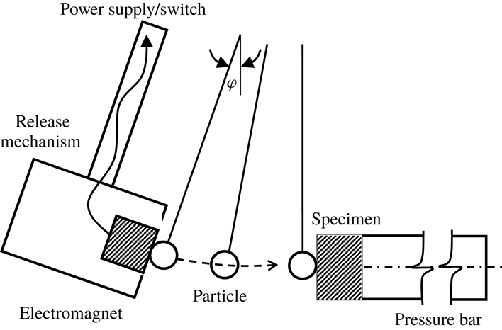
The experimental set-up shown in figure 1 is similar to that used by Ruiz-Angulo & Hunt (Reference Ruiz-Angulo and Hunt2010). The experiments are designed to measure the surface deformation (residual crater diameter and depth) and rebound velocity of a single particle impacting a wall. The collisions occur in air and in six different water–glycerol mixtures. A glass tank contains the fluid, the particle release mechanism, the impact sample and the pressure bar.
Schematic representation of the experimental apparatus (after Ruiz-Angulo & Hunt (Reference Ruiz-Angulo and Hunt2010)).

The impact speed is varied by changing the particle release angle
 $\unicode[STIX]{x1D711}$
; the particle follows a pendulum-like trajectory with negligible rotation impacting perpendicular to the impact surface. The impact velocities range from approximately
 $1~\text{cm}~\text{s}^{-1}$
in the most viscous fluid up to approximately
 $45~\text{cm}~\text{s}^{-1}$
in air. The particle trajectory is recorded with a high-speed camera with recording rates ranging from 500 to 1000 frames per second. The images are post-processed to track the particle trajectories and estimate the impact and rebound velocities (
 $u_{i}$
and
 $u_{r}$
) for each collision, which are used to compute the coefficient of restitution,
 $e=-u_{r}/u_{i}$
. As a note, the velocity variation due to particle impact can occur over time scales that are smaller than can be resolved by the camera.
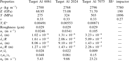
The impact particle is a highly spherical, hard stainless steel sphere with diameter 12.7 mm. Relative to the impactor, the three impact surfaces are softer aluminium alloys (6061, 2024 and 7075). Table 1 lists properties of the particle and impact surfaces (
 $\unicode[STIX]{x1D70C}$
,
 $E$
,
 $Y$
and
 $\unicode[STIX]{x1D708}$
) and the root mean square (r.m.s.) surface roughness. The values of the yield speeds for each alloy and the corresponding depth and radius of the indentation at yield (
 $\unicode[STIX]{x1D6FF}_{y}$
and
 $a_{y}$
) are found in table 1, as well as their values normalized by the particle radius (
 $\unicode[STIX]{x1D6FF}_{y}/R$
and
 $a_{y}/R$
). Yielding is assumed to occur when
 $\unicode[STIX]{x1D70E}_{el}=C_{y}Y$
, where
 $C_{y}$
is a constant determined from von Mises yield criterion; here,
 $C_{y}=1.65$
for three alloys with
 $\unicode[STIX]{x1D708}=0.33$
(Jackson & Green Reference Jackson and Green2005). The yield speed is the largest for the 7075 alloy, which has the largest ratio of
 $Y/E^{\ast }$
as found in table 1. Also listed is an estimate of the impact velocity that corresponds to the onset of plastic deformations,
 $u_{p}$
, assuming that
 $P_{d}=2.8Y$
and
 $\unicode[STIX]{x1D700}=a_{p}/a_{y}=13$
. In addition, table 1 includes the ratio of the surface roughness to
 $\unicode[STIX]{x1D6FF}_{y}$
for each of the alloys, showing that the roughness is much smaller than the indentation depth at the critical yield speed.
Mechanical properties of target surfaces, the spherical impactor, the r.m.s. height of surface roughness for impacted surface and calculated properties at yield and the onset of plastic deformation;
 $^{+}$
SS stands for stainless steel.

The elastic collision time can be estimated from (2.7) and ranges from
 $19\times 10^{-6}$
to
 $26\times 10^{-6}$
s for
 $u_{i}=u_{y}$
for the 7075 and 6061 alloys, respectively. Table 1 lists the elastic collision time normalized by a hydrodynamic transit time,
 $\unicode[STIX]{x1D70F}_{e}/(x_{o}/u_{y})$
, using the yield speed. The transit time is estimated from the time required for a particle to move a distance
 $x_{o}$
at a constant speed. This time is considerably shorter than the fluid contact times that include fluid inertia or viscous drag as proposed by Legendre et al. (Reference Legendre, Zenit, Daniel and Guiraud2006) and Kempe & Frohlich (Reference Kempe and Frohlich2014); hence, the transit time provides a lower bound for the time constant associated with the fluid effects. As found in the table for the 6061 and 2024 alloys, the elastic collision time is significantly shorter than the transit time; for the 7075 alloy the two times are closer because of the larger value of
 $u_{y}$
.
The experiments involve a split-Hopkinson–Kolsky pressure bar arrangement in which a cylindrical impact specimen (2.54 cm diameter and 12.7 mm thickness) is attached to a long pressure bar. The bar (approximately 30 cm) is long enough that the contact time between the particle and the specimen is shorter than the time an elastic wave takes to travel the bar length back and forth (propagation and reflection) to the point of impact. Prior to each experiment, the samples are firmly attached to the transmission bar using a glycerin-based lubricant between the sample and the transmission bar to mechanically couple the two. The plane wave propagates without distortion through the sample and the bar. In preliminary experiments, a force sensor was used to monitor the contact force and contact time between the particle and the bar with and without the sample. Those experiments showed that the collision time did not change with the presence of the sample (Ruiz-Angulo & Hunt Reference Ruiz-Angulo and Hunt2010).
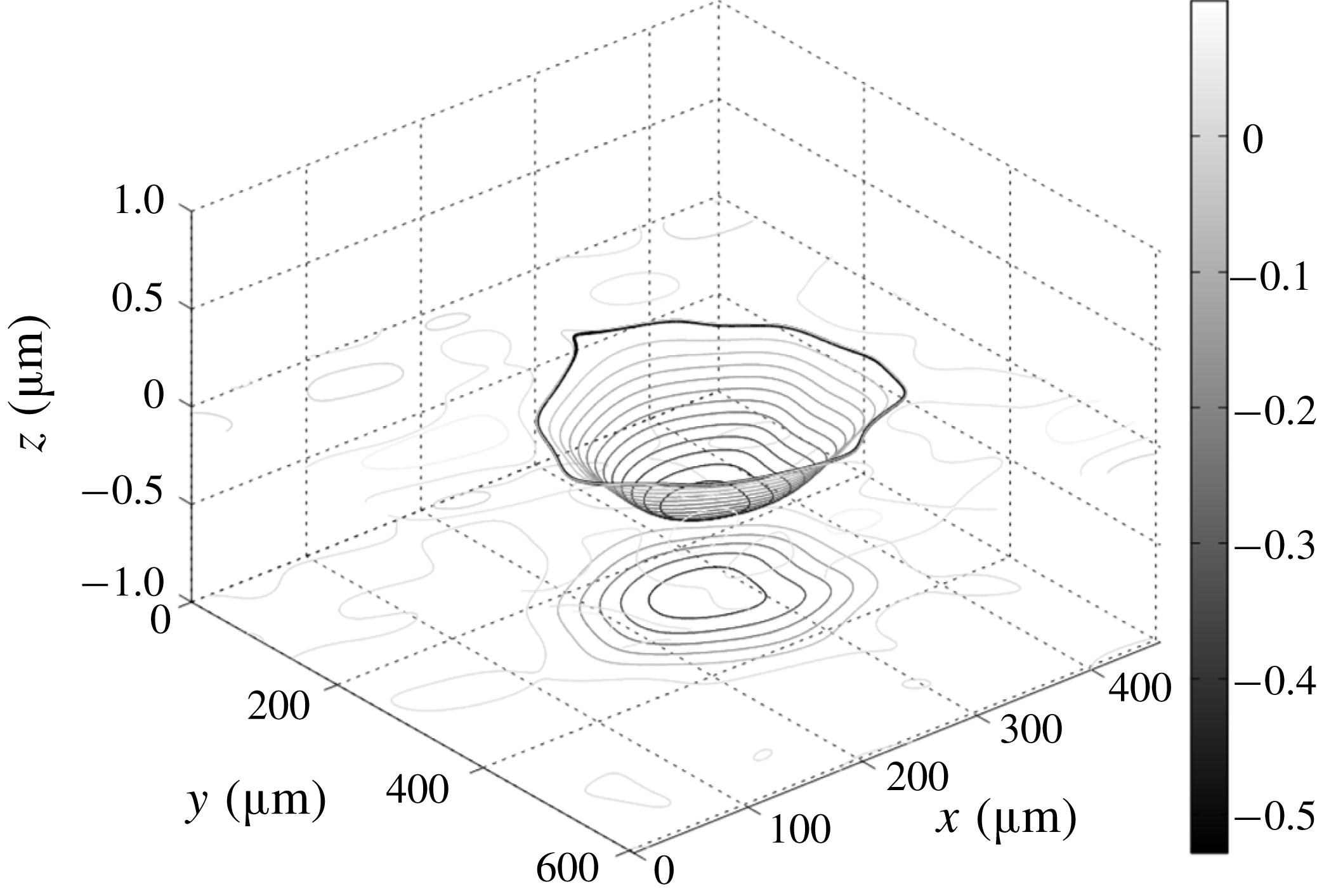
Three-dimensional contours and their respective
 $x$
–
 $y$
projections for the indentation corresponding to a 6061 aluminium alloy specimen impacted at a speed of
 $0.179~\text{m}~\text{s}^{-1}$
by the stainless steel particle while submerged in fluid WG6. The thick black curves represent the best-fitted contours.

Before running each experiment, the impact sample is ground and polished using water-based suspensions of polycrystalline diamond. The impact surfaces have a mirror finish with roughness of
 $0.029~\unicode[STIX]{x03BC}\text{m}$
and root mean square variation of
 $0.028~\unicode[STIX]{x03BC}\text{m}$
, as measured with the profilometer. Each experiment uses a new impact sample. After each collision, the sample is removed from the pressure bar and the deformed surface is analysed using a WYKO optical profilometer. The three-dimensional surface profiles are low pass filtered to remove the roughness. The indentations are then fitted with curves to determine the residual crater diameter
 $d_{r}$
and the residual crater depth
 $\unicode[STIX]{x1D6FF}_{r}$
. The errors in the measurements of the indentation parameters are associated with the difference between the filtered contours and the idealized geometry to which the crater diameter was optimally fitted. Figure 2 shows an example of the three-dimensional contours that are fitted to the crater formed after the sphere impacted the 6061 alloy at a speed of
 $0.179~\text{m}~\text{s}^{-1}$
in the WG6 fluid. For this case, the measured depth is
 $0.584~\unicode[STIX]{x03BC}\text{m}$
, the diameter is
 $260~\unicode[STIX]{x03BC}\text{m}$
and the corresponding coefficient of restitution is 0.32.
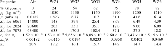
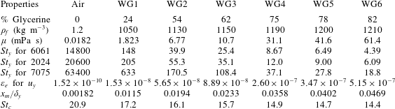
The collision experiments were performed in air and in six different aqueous–glycerol solutions ranging from 24 % glycerol and 76 % water (based on mass and labelled WG1) to 82 % glycerol and 18 % water (labelled WG6). Table 2 includes the values of density and dynamic viscosity of these fluids along with the Stokes number at the yield speed,
 $St_{y}=2R\unicode[STIX]{x1D70C}u_{y}/(9\unicode[STIX]{x1D707})$
, for all alloys in each of the fluids. Also included in table 2 is the minimum distance of approach to the wall normalized by the yield crater depth, as estimated from
 $x_{m}\approx (1/4)x_{o}\unicode[STIX]{x1D700}_{e}^{2/5}$
using
 $x_{o}=R/100$
and
 $u_{o}=u_{y}$
for aluminium 6061. For this case and other collisions, the minimum distance of approach is considerably smaller than
 $\unicode[STIX]{x1D6FF}_{y}$
; hence, the thickness of the lubrication layer is small relative to the indentation depth for the 6061 alloy as well as the 2024 and 7075 alloys. The table also includes an estimate for the critical Stokes number for the 6061 alloy using
 $St_{c}=2\ln (x_{o}/x_{m})$
. The estimated values for
 $St_{c}$
for all of the alloys are in the range from 14 to 20 and are consistent with prior experimental measurements (Joseph et al.
Reference Joseph, Zenit, Hunt and Rosenwinkel2001).
Physical properties for the fluids used in this study and the Stokes number at the yield speed for all alloys. The value of
 $\unicode[STIX]{x1D700}_{e}$
, the minimum distance between the impacting particle and the surface and an estimate of the critical Stokes number based on the minimum distance of approach are evaluated for the 6061 alloy.
4 Experimental results and discussion
4.1 Results of collisions without viscous losses (in air)
Before examining collisions with a liquid, it is useful to examine the collision process in air with negligible viscous loss. Figure 3 shows the coefficient of restitution for all alloys as a function of
 $U^{\ast }=u_{i}/u_{y}$
. For each alloy, the impact speed varies over a similar range (roughly
 $0.02~\text{m}~\text{s}^{-1}$
to
 $0.5~\text{m}~\text{s}^{-1}$
). Because of the different values of
 $u_{y}$
, the range of
 $U^{\ast }$
is lower for the harder 7075 aluminium alloy than for the softer 6061 aluminium alloy.
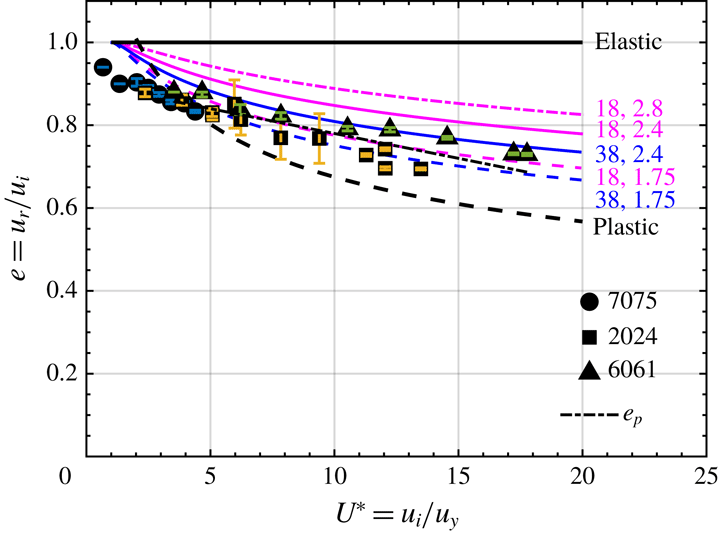
The coefficient of restitution decreases from unity (elastic collisions) with increasing
 $U^{\ast }$
. Ruiz-Angulo & Hunt (Reference Ruiz-Angulo and Hunt2010) report the estimated errors in measuring the coefficient of restitution. As shown in figure 3, the fully plastic model (dashed black),
 $e=1.2U^{\ast -1/4}$
, overestimates the drop in
 $e$
for most of the impact speeds. The factor 1.2 is obtained from (2.13) with
 $\unicode[STIX]{x1D713}=2.8$
and
 $C_{y}=1.65$
. It is noteworthy that the ratio of
 $u_{p}/u_{y}$
is roughly 250 for all alloys; hence, the impact speeds in these experiments (with
 $U^{\ast }<20$
) are in the elastic and elastic–plastic regimes and correspond to impact speeds considerably smaller than those required for fully plastic impacts.
Coefficient of restitution versus impact velocity normalized by the yield velocity in air. Data points are from this study on three aluminium alloys. Curves are the model suggested by Ma & Liu (Reference Ma and Liu2015) with five sets of
 $\unicode[STIX]{x1D713}$
and
 $\unicode[STIX]{x1D700}$
. Trends for collisions involving elastic (
 $e=1$
), plastic (
 $e=1.2U^{\ast -1/4}$
) and the best fit curve (
 $e=0.9{-}0.012U^{\ast }$
) are shown. The size of error bars is smaller than the size of symbols on the majority of data points.

The coefficient of restitution based on the elastic–plastic models of Ma & Liu (Reference Ma and Liu2015) is also shown in figure 3 for five different combinations of parameters
 $\unicode[STIX]{x1D700}=\{18,38\}$
and
 $\unicode[STIX]{x1D713}=\{1.75,2.4,2.8\}$
. The experimental results fit best by the curve associated with
 $\unicode[STIX]{x1D700}=18$
and
 $\unicode[STIX]{x1D713}=1.75$
. These values correspond to large areas (
 $\unicode[STIX]{x1D700}=a_{p}/a_{y}:[13-20]$
) and lower hardness (
 $\unicode[STIX]{x1D713}=1.75\ll 2.8{-}3$
) than typically used to model elastic–plastic behaviour. The work by Ma & Liu (Reference Ma and Liu2015) also used larger values for
 $\unicode[STIX]{x1D700}$
when the two bodies had very different yield strengths, as is the case in the present experiments. Note that the yield strength of the impactor is 4–7 times large than that of the target alloys. Although not shown, the results were also compared to the elastic–plastic model by Stronge (Reference Stronge2000), which assumed a fully plastic collision equivalent to
 $\unicode[STIX]{x1D700}=13$
and
 $\unicode[STIX]{x1D713}=2.8$
; these results did not capture the variation in the coefficient of restitution as a function of
 $U^{\ast }$
as measured in this study.
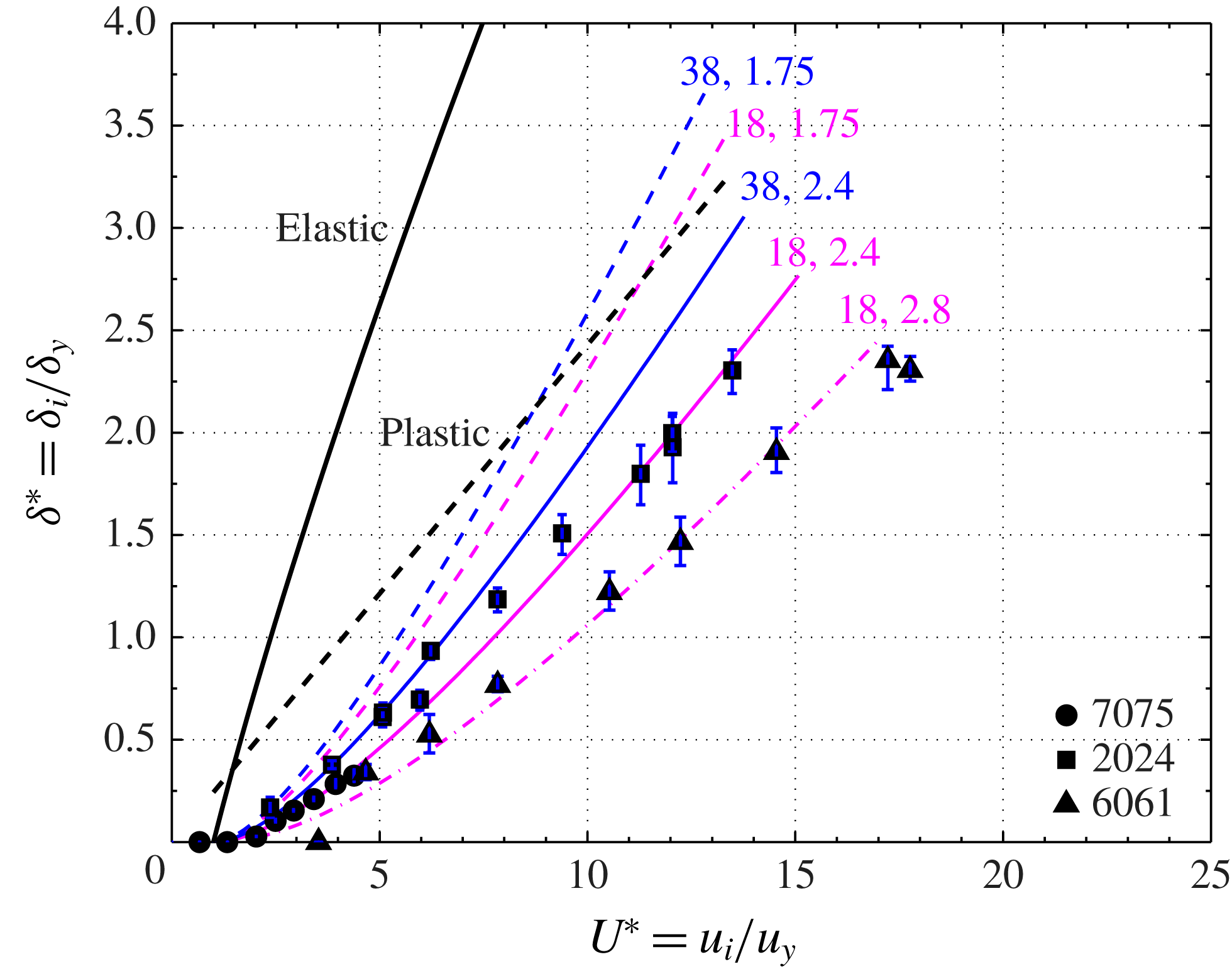
Residual crater depth normalized by the yield depth versus impact velocity normalized by the yield velocity (2.4). Data points are from this study corresponding to collisions against three different aluminium alloys in air. Coloured curves correspond to the model developed by Ma & Liu (Reference Ma and Liu2015) labelled with five sets of parameters
 $\unicode[STIX]{x1D700}=\{18,38\}$
and
 $\unicode[STIX]{x1D713}=\{1.75,2.4,2.8\}$
. Solid and dashed black lines show the elastic and plastic deformations resulting from equations (2.6) and (2.10), respectively. The size of error bars is smaller than the size of symbols on the majority of data points.

Figures 4 and 5 show the measured residual indentation depth and diameter normalized by the values at the onset of yielding, respectively, in terms of the normalized impact velocity,
 $U^{\ast }$
, for the three alloys colliding in air. As shown in both figures, the measurements for 6061 and 7075 alloys collapse along similar trends with slightly higher values for the 2024 alloy, especially, for the residual indentation depth. From the figures, the lowest impact speed for a measurable crater is at
 $U^{\ast }\approx 2$
, which is at a speed roughly twice the yield speed. This onset of an observable crater formation agrees with the elastic–plastic numerical simulations by Jackson & Green (Reference Jackson and Green2005), showing that the onset of plastic deformation initiates below the surface at
 $U^{\ast }\approx 1$
and appears at the surface for
 $U^{\ast }\geqslant 2$
.
The Ma & Liu (Reference Ma and Liu2015) prediction for
 $\unicode[STIX]{x1D713}=2.4$
and
 $\unicode[STIX]{x1D700}=18$
is closer to the experimental data in figure 4. However, that combination of parameters did not adequately capture the variation for the coefficient of restitution (figure 3). It is unclear why different parameters are needed to fit these two different sets of experiments. The Ma & Liu (Reference Ma and Liu2015) study was used to predict coefficients of rebound; this study did not compare predictions with residual crater dimensions from experiments. Other recent studies on elasto–plastic behaviour of materials suggest that other factors (such as strain-rate-dependent properties and work hardening) may need to be incorporated in elasto–plastic contact laws to adequately predict experimental data (Wang et al.
Reference Wang, Geubelle and Lambros2013; Burgoyne & Daraio Reference Burgoyne and Daraio2014). In figure 4, the elastic line corresponds to
 $\unicode[STIX]{x1D6FF}_{e}/\unicode[STIX]{x1D6FF}_{y}-1=U^{\ast 4/5}-1$
, which extrapolates the scaling from the elastic regime into the elastic–plastic regime and forces
 $\unicode[STIX]{x1D6FF}_{e}/\unicode[STIX]{x1D6FF}_{y}=1$
(or
 $\unicode[STIX]{x1D6FF}_{r}=0$
) at
 $U^{\ast }=1$
. The plastic curve corresponds to
 $\unicode[STIX]{x1D6FF}_{p}/\unicode[STIX]{x1D6FF}_{y}=[C_{y}/(10\unicode[STIX]{x1D713})]^{1/2}U^{\ast }$
with
 $\unicode[STIX]{x1D713}=2.8$
and
 $C_{y}=1.65$
. Both the elastic and plastic scalings overestimate the measured residual crater depth.
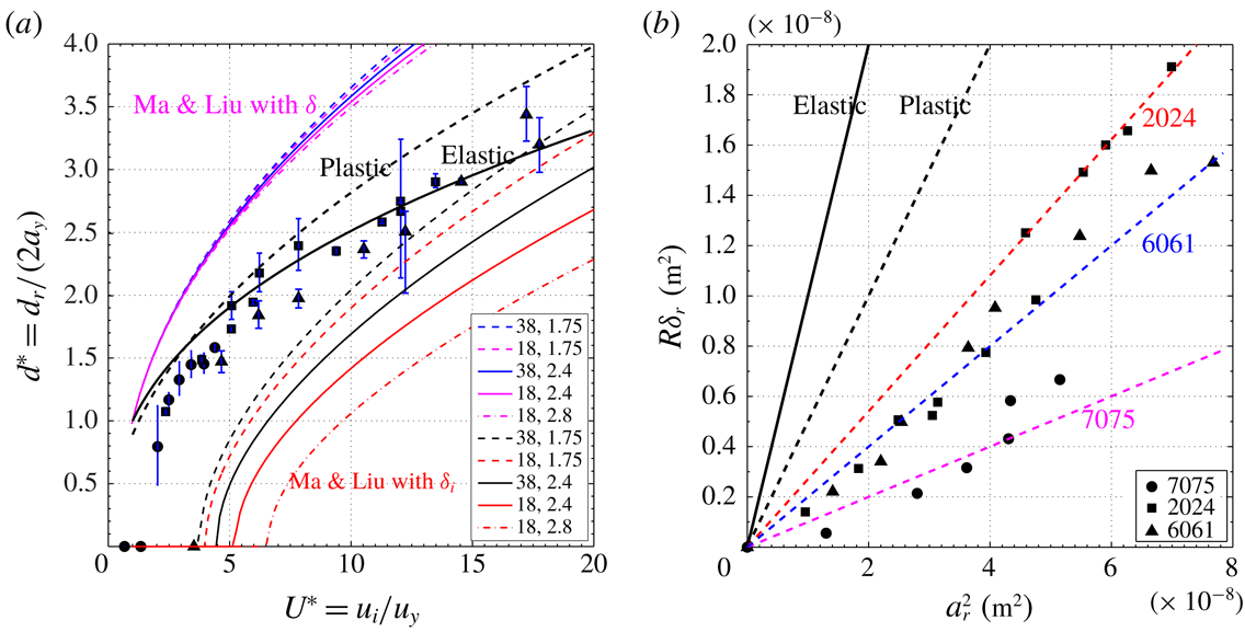
In figure 5, the normalized crater diameters are captured best by the curve that extrapolates the linear elasticity results beyond
 $U^{\ast }=1$
with
 $d_{e}/(2a_{y})=U^{\ast 2/5}$
. The curve for plastic behaviour corresponding to
 $d_{r}/(2a_{y})=[16C_{y}/(15\unicode[STIX]{x1D713})]^{1/4}U^{\ast 1/2}$
(with
 $\unicode[STIX]{x1D713}=2.8$
and
 $C_{y}=1.65$
) overestimates the experimental data. Ma and Liu assumed the relation,
 $a_{r}=[(2\unicode[STIX]{x1D6FF}-\unicode[STIX]{x1D6FF}_{y})R]^{1/2}$
. Using this expression, the predicted crater diameter does not correspond well with the experimental measurements in figure 5(a) using the same set of parameters,
 $\unicode[STIX]{x1D713}$
and
 $\unicode[STIX]{x1D700}$
, as used in figures 3 and 4. A second set of curves is also shown using
 $a_{r}=[(2\unicode[STIX]{x1D6FF}_{r}-\unicode[STIX]{x1D6FF}_{y})R]^{1/2}$
. Note that in the second set of curves (plotted lower in the graph), the residual crater depth is used to obtain the residual crater diameter, but in the first set (upper plots in the graph), the total depth is used. Both sets of curves fall outside the elastic and plastic trends and off the experimental data acquired in this study for collisions in air.
Figure 5(b) shows the residual crater depth multiplied by the particle radius
 $R\unicode[STIX]{x1D6FF}_{r}$
versus the residual crater radius squared
 $a_{r}^{2}$
. The measured values for collisions in air follow neither the elastic (slope of 1) nor the plastic (slope of
 $1/2$
) trends. Instead, the measurements show lower slopes with a slope of
 $1/10$
for 7075,
 $1/5$
for 6061, and
 $1/3.7$
for 2024. A line fitted to all the data has a slope of
 $1/4$
. If the craters are assumed to result from a spherical impactor, the effective radius of the impactor,
 $R_{i}$
, can be estimated as
 $R_{i}=(\unicode[STIX]{x1D6FF}_{r}^{2}+a_{r}^{2})/2\unicode[STIX]{x1D6FF}_{r}$
. Using
 $R\unicode[STIX]{x1D6FF}_{r}=Aa_{r}^{2}$
where
 $A$
is the slope found in figure 5(b), the effective radius of the impactor is
 $R_{i}/R=1/(2A)$
, which gives
 $R_{i}/R=5$
for the 7075 alloy, 2.5 for the 6061 alloy and 1.85 for the 2024 alloy. Hence for these elastic–plastic collisions the steel impactor produces craters significantly shallower than expected from pure plasticity theory or extrapolated from Hertz theory. As a note the experiments by Wang et al. (Reference Wang, Geubelle and Lambros2013) also found that the residual crater depth increases linearly with the residual crater area; the slope of the data varied with material and was also significantly smaller than predicted by a Hertz model. As described in Johnson (Reference Johnson1985) for a hard impactor hitting a softer target, the indentation under load can have a higher effective radius because of the elastic compression of the impactor; when the load is removed the indentation shallows due to elastic recovery so the curvature of the residual crater is greater than the radius of the impactor.
The uncertainly in the measured depth and diameter are determined from the quality of the fit of the measured shape to the idealized form including a threshold that could underestimate the measurement. The deviation of the fitted shape to a spherical surface could be up to ten per cent of the reported diameter of the crater and approximately five per cent of the reported depth.
(a) Residual crater diameter (
 $d_{r}$
) normalized by the yield diameter (
 $2a_{y}$
) versus impact velocity (
 $u_{i}$
) normalized by the yield velocity (
 $u_{y}$
). Data points are from this study for three different aluminium alloys collided with by the particle while surrounded by air. Coloured curves correspond to the model proposed by Ma & Liu (Reference Ma and Liu2015) labelled accordingly with the sets of parameters
 $\unicode[STIX]{x1D700}=\{18,38\}$
and
 $\unicode[STIX]{x1D713}=\{1.75,2.4,2.8\}$
shown in the legend. The lower set of curves located are calculated with the residual crater depth; the upper set of curves are calculated with the total crater depth. Trends for collisions involving elastic and plastic deformations, equations (2.6a
) and (2.11a
), are the solid and dashed black curves, respectively. The size of error bars is smaller than the size of symbols for the majority of data points. (b) Elastic and plastic expressions for residual crater depth (
 $\unicode[STIX]{x1D6FF}_{r}$
) times the particle radius (
 $R$
) as a function of the residual crater radius squared and experimental measurements for collisions in air. The slopes of the lines are
 $1/3.7$
,
 $1/4$
and
 $1/10$
.

4.2 Results of collisions with viscous losses (in a liquid)
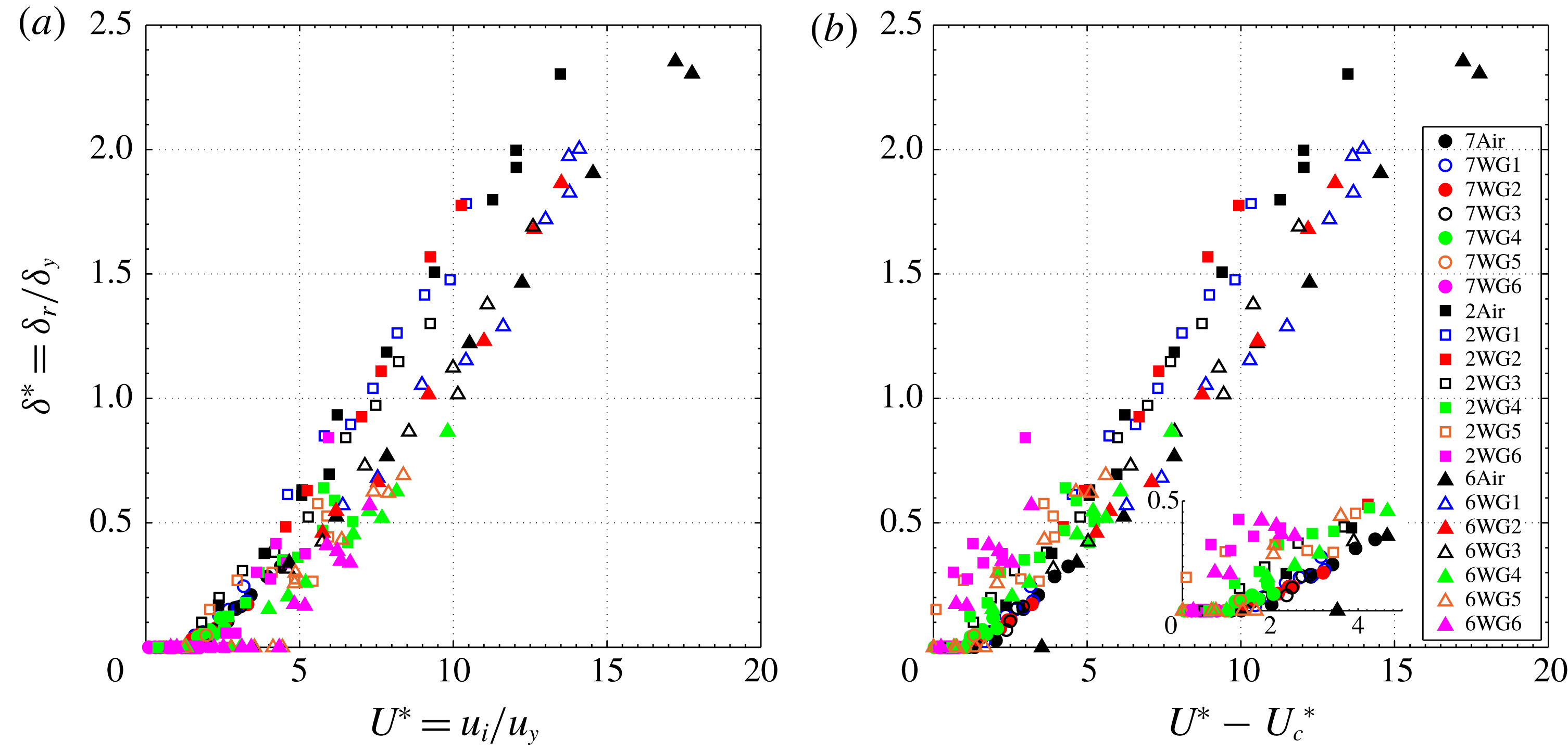
As described earlier, the experiments were also conducted with six different glycerin–water mixtures (labelled WG1 to WG6) to provide a range of fluid properties as found in table 2. Figure 6(a) shows the measurements for the normalized residual depth of the crater as a function of
 $U^{\ast }$
for all alloys in the six different liquids. For comparison, the data for collisions in air are also shown. The results show that the viscous fluid does not have a significant effect on the crater dimensions as all the data follow a similar trend. As mentioned earlier, the minimum approach distance at the yield speed and the surface roughness compared to the yield crater depth,
 $x_{m}/\unicode[STIX]{x1D6FF}_{y}$
and
 $\unicode[STIX]{x1D70E}/\unicode[STIX]{x1D6FF}_{y}$
(table 2), are much less than 1. Although the current experiments do not determine whether there is direct solid-to-solid impact between the surfaces, these length scales suggest that the fluid volume between the particle and the wall at the closest approach or at the roughness height is significantly smaller than the volume of the indentation. As a result, the surrounding fluid has minimal impact on the size of the crater.
(a) Normalized crater depth versus normalized impact velocity,
 $U^{\ast }$
, for collisions in seven different fluids. (b) Normalized crater depth plotted as a function of reduced velocity
 $U^{\ast }-U_{c}^{\ast }$
using
 $St_{c}=18$
. Note: in the legend, the alloys are represented by the first number in their names: 7 for 7075, 2 for 2014 and 6 for 6061.

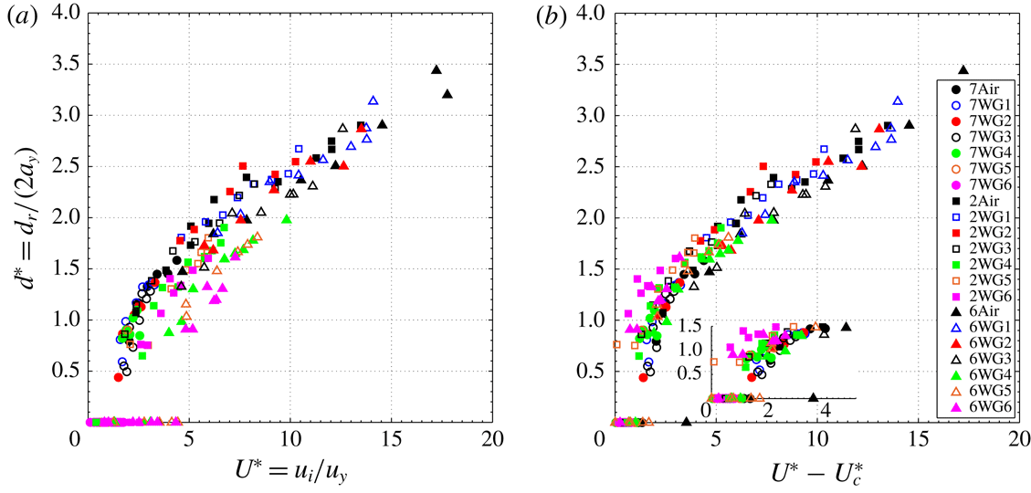
Figure 7(a) shows the measured normalized crater diameters for all alloys versus
 $U^{\ast }$
. Consistent with figure 6(a), the trends do not vary significantly with the surrounding fluid. At these speeds, the crater diameters are slightly smaller than that calculated from Hertz theory. Like the collisions in air, the diameters increase with impact speed at approximately
 $U^{\ast 2/5}$
(similar to the elastic trend), especially at the higher speeds. At the lower speeds, the collisions for alloys 6061 and 2024 in the more viscous fluids (WG5 and WG6) have slightly smaller diameters than found for the less viscous fluids. For the harder 7075 alloy, there were no measurable craters for the WG6 experiments and only one experiment produced a crater in WG5.
(a) Normalized crater diameter versus normalized impact velocity,
 $U^{\ast }$
, for all the collisions in the different fluids. (b) Normalized crater diameter plotted as a function of reduced velocity
 $U^{\ast }-U_{c}^{\ast }$
using
 $St_{c}=18$
.

The speed at which a permanent crater first appears depends on the combination of materials. For the hardest material (Al-7075), cratering begins at
 $U^{\ast }\approx 2$
, consistent with the results for air. Cratering begins at
 $U^{\ast }\approx 3$
for the 2024 alloy and at
 $U^{\ast }\approx 4$
for 6061 alloy. The differences for the onset is linked to the impact velocity and the yield velocity. Using
 $U^{\ast }$
, the Stokes number for a given experiment can be calculated from the value of
 $St_{y}$
(found in table 2) as
 $St=St_{y}U^{\ast }$
. As previously discussed, the critical Stokes number,
 $St_{c}$
has been used to determine when a particle has sufficient incoming kinetic energy to overcome viscous losses during an elastic collision and rebound from the surface. Moreover, if
 $St<St_{c}$
, the particle does not have sufficient kinetic energy to cause plastic deformation. In the prior work by Ruiz-Angulo & Hunt (Reference Ruiz-Angulo and Hunt2010), they assumed that the critical Stokes number was
 $St_{c}\approx 18$
for all three alloys. For the 7075 alloy and the WG6 fluid, the Stokes number at yield is
 $St_{y}=18.8$
(see table 2). Hence, for
 $U^{\ast }=2$
,
 $St=37.6$
, which is greater than
 $St_{c}$
; as a result, a particle at
 $U^{\ast }=2$
has enough kinetic energy to overcome viscous losses during impact and potentially enough to leave a crater on the 7075 alloy. For the 6061 and the 2024 alloys at
 $U^{\ast }=2$
, the corresponding Stokes numbers for WG6 are
 $St=8.8$
and
 $St=12.2$
, respectively, both below
 $St_{c}$
. As a result, these impacts are not expected to generate a crater during impact, and they did not. With these considerations, the data found in figures 6(a) and 7(a) are represented in terms of
 $U^{\ast }-U_{c}^{\ast }=U^{\ast }-St_{c}/St_{y}$
in figures 6(b) and 7(b). The re-scaling brings the data closer together, such that the experiments without crater formation correspond to
 $U^{\ast }-U_{c}^{\ast }<2$
or as
 $St-St_{c}<2St_{y}$
; this scaling demonstrates that the impact kinetic energy is reduced because of the viscous losses during the approach of the particle to the surface. The value of
 $U_{c}^{\ast }$
for all three alloys and all fluid uses
 $St_{c}=18$
.
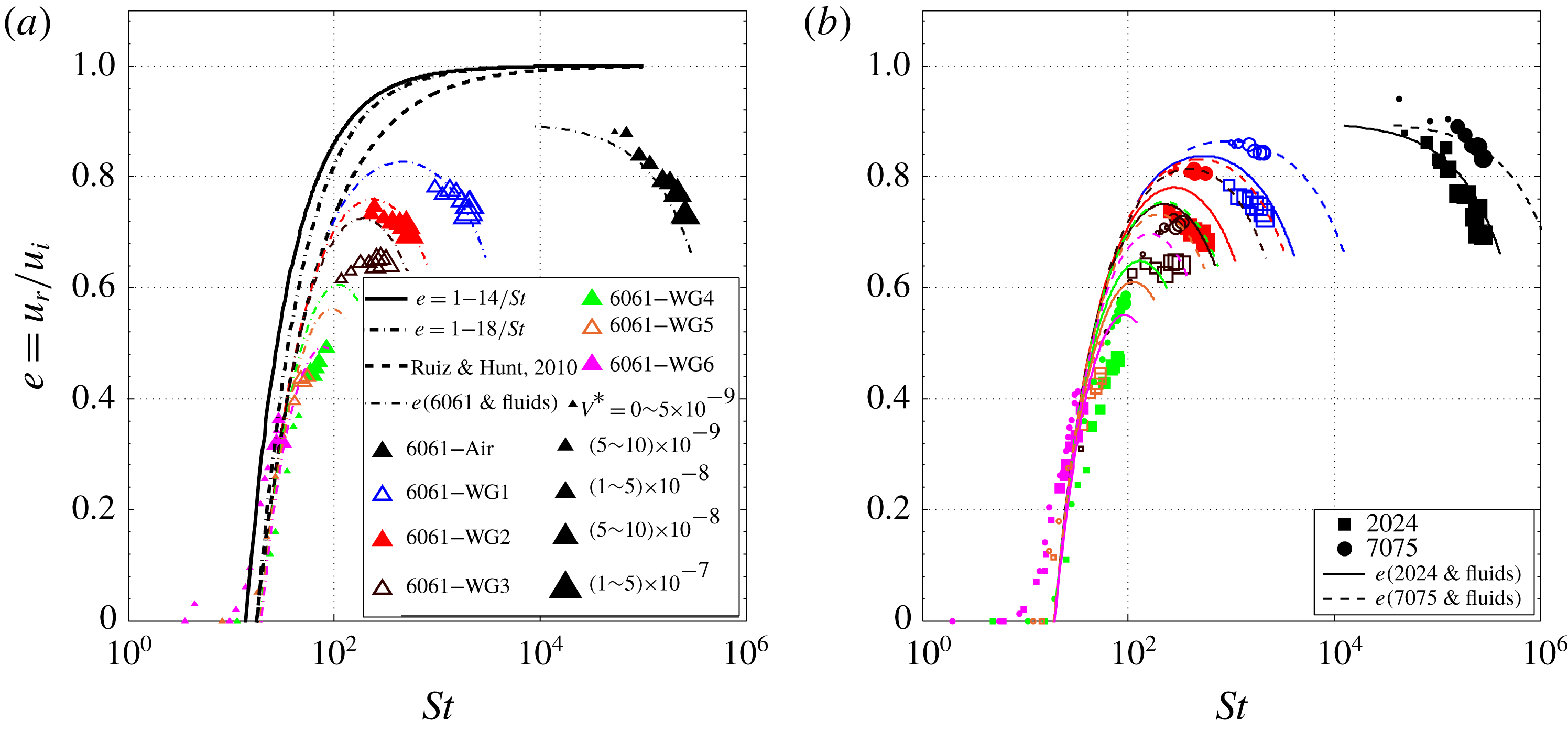
Figure 8(a) presents the measured coefficients of restitution as a function of Stokes number for the Al-6061 alloy in all fluids. The coefficient of restitution increases with Stokes number up to a maximum value that depends on the fluid and then decreases due to plasticity effects. The size of the symbols is proportional to the crater volume normalized by the particle volume,
 $V^{\ast }=V_{r}/V_{s}$
. The thick black solid and dash-dotted lines correspond to
 $e=1-St_{c}/St$
and using
 $St_{c}=14$
and
 $18$
, respectively. The thick dashed line represents the expression developed by Ruiz-Angulo & Hunt (Reference Ruiz-Angulo and Hunt2010) that also neglects the particle inelasticity:
 $e=1-8.75/St^{0.75}$
. For relatively high Stokes numbers, the experimental data points fall away from these curves, especially as the plasticity effects become important, as quantified by the size of the crater. The thin coloured dash-dotted curves in figure 8(a) include the inelasticity of the impacting objects, using a modified version of (2.19) and allowing the value of
 $e_{p}$
to depend on the value of
 $U^{\ast }$
,
 $$\begin{eqnarray}e=e_{p}-(1+e_{p})\frac{St_{c}}{2St}.\end{eqnarray}$$
The value of 2 is included in the denominator so that
 $e=0$
when
 $St=St_{c}$
and
 $e_{p}=1$
. For each fluid, the value of
 $e_{p}$
can be calculated based on the measurements in air, which depend on the value of
 $U^{\ast }=St/St_{y}$
. To simplify the evaluation of
 $e_{p}$
, a linear curve was fit to the data of
 $e_{p}$
for the three alloys colliding in air as found in figure 3 with
 $e_{p}=0.9{-}0.012U^{\ast }$
. As shown in figure 8, the curves roughly capture the data for each fluid, especially for the less viscous fluids such as WG1, WG2 and WG3. The Stokes number that corresponds with the maximum coefficient of restitution can be estimated by using the equation,
 $e=(0.9-0.012U^{\ast })-(1.9-0.012U^{\ast })St_{c}/(2St_{y}U^{\ast })$
, differentiating with respect to
 $U^{\ast }$
and setting the derivative equal to 0. The maximum coefficient of restitution occurs at
 $St=8.9(St_{c}\times St_{y})^{0.5}$
, which is approximately 460 for WG1, 240 for WG2, 190 for WG3, 110 for WG4, 96 for WG5 and 79 for WG6. As a note, the value of
 $e_{p}$
was also calculated using
 $U^{\ast }-U_{c}$
rather than
 $U^{\ast }$
; this method slightly improves the correspondence with the experimental data. This analysis, which assumes that the plastic deformation occurs instantaneous relative to the viscous dissipation (Birwa et al.
Reference Birwa, Rajalakshmi, Govindarajan and Menon2018), works well at the higher Stokes numbers (corresponding with WG1, WG2 and WG3) but does not capture all of the plastic losses for Stokes numbers near 100 (corresponding with WG4, WG5 and WG6) where the viscous and plasticity effects may be harder to separate.
Coefficient of restitution versus Stokes number for (a) 6061 aluminium alloy. (b) 2024 and 7075 alloys. Experimental data points are represented with triangles for 6061, squares for 2024 and circles for 7075. The size of data symbols is proportional to the crater volume normalized by the particle volume. The colour code is consistent in all alloy–fluid combinations as summarized in the legend. Curves correspond to different fits and proposed models using
 $St_{c}=18$
.

Figure 8(b) shows corresponding data for the 2024 and 7075 alloys using (4.1). Also shown are the predictions for
 $e$
for these alloys. The results for these alloys are similar to those found for the 6061 alloy and the predictions of the measurements correspond best with the results for the higher Stokes numbers.
4.3 Applications to erosion studies
As described in the introduction, the erosion rate is measured in either the volume or the mass lost per unit time or per the number of particle impacts. For a single normal collision, Bitter (Reference Bitter1963a
,Reference Bitter
b
) proposed the following expression for the wear,
 $W_{d}$
, which is the volume loss per particle impact involving a particle of mass
 $m$
colliding with a deformable surface and
 $E_{v}$
is the amount of energy needed to remove one unit of volume:
 $$\begin{eqnarray}W_{d}=\frac{\displaystyle m(u_{i}-u_{y})^{2}}{\displaystyle 2E_{v}}.\end{eqnarray}$$
Here, Bitter argued that
 $E_{v}$
depends on the properties of the impacted surface and reflects the amount of energy per volume required for elastic–plastic deformation. The experiments by Bitter (Reference Bitter1963a
) used hardened steel balls impacting both ductile (low-carbon steel) and brittle (plastics and glass) materials. Bitter (Reference Bitter1963a
,Reference Bitter
b
) argued that
 $E_{v}$
should be proportional to
 $\unicode[STIX]{x1D70E}_{el}^{2}/E^{\ast }$
with
 $\unicode[STIX]{x1D70E}_{el}=C_{y}Y$
and
 $C_{y}$
being between 1.6 to 3.2 depending on the work hardening of the material. Sklar & Dietrich (Reference Sklar and Dietrich2004) modified Bitter’s wear model by writing the right-hand side of (4.2) as
 $((1/2)mu_{i}^{2}-E_{t})/E_{v}$
, where
 $E_{t}$
accounts for the threshold energy that must be exceeded for material detachment to occur. In comparing with experiments involving sediment and water in an abrasion mill, they neglect the
 $E_{t}$
term and experimentally determine appropriate values of
 $E_{v}$
. In the recent studies by Lamb et al. (Reference Lamb, Dietrich and Sklar2008) and Scheingross et al. (Reference Scheingross, Brun, Lo, Omerdin and Lamb2014), the authors used modelling based on Bitter’s analysis and included the effects of viscous damping by selecting a cutoff Stokes number below which erosion did not occur.
In the analysis below, expressions are developed for the residual crater volume normalized by the particle volume based on elastic and plastic theories and from the experimental measurements. By considering a spherical shape for the indentation, its volume can be computed from
 $V_{r}=\unicode[STIX]{x03C0}\unicode[STIX]{x1D6FF}_{r}(3/4d_{r}^{2}+\unicode[STIX]{x1D6FF}_{r}^{2})/6\approx \unicode[STIX]{x03C0}\unicode[STIX]{x1D6FF}_{r}a_{r}^{2}/2$
. For a plastic collision,
 $\unicode[STIX]{x1D6FF}_{p}=a_{p}^{2}/(2R)$
; the residual deformed volume,
 $V_{r}$
, normalized by the volume of a sphere,
 $V_{s}$
, is
 $V^{\ast }=V_{r}/V_{s}\approx 3/4(\unicode[STIX]{x1D6FF}_{r}/R)^{2}$
. For a plastic collision, the volume ratio can be estimated using (2.10b
) as follows:
 $$\begin{eqnarray}\frac{\displaystyle V_{r}}{\displaystyle V_{s}}\approx \frac{\displaystyle 3}{\displaystyle 4}\left(\frac{\displaystyle \unicode[STIX]{x1D6FF}_{p}}{\displaystyle R}\right)^{2}=\frac{\displaystyle 3}{\displaystyle 4}\left(\frac{\displaystyle 2\unicode[STIX]{x1D70C}u_{y}^{2}}{\displaystyle P_{d}}\right)U^{\ast 2}=\frac{\displaystyle 3\unicode[STIX]{x03C0}^{4}}{\displaystyle 80}\frac{\displaystyle C_{y}^{5}}{\displaystyle \unicode[STIX]{x1D713}}\left(\frac{\displaystyle Y}{\displaystyle E^{\ast }}\right)^{4}U^{\ast 2}=15.9\left(\frac{\displaystyle Y}{\displaystyle E^{\ast }}\right)^{4}U^{\ast 2}.\end{eqnarray}$$
A similar expression can be found using the scaling for an elastic collision by estimating the normalized volume as
 $V^{\ast }=V_{r}/V_{s}\approx 3/8(\unicode[STIX]{x1D6FF}_{r}/R)^{2}$
, which uses
 $\unicode[STIX]{x1D6FF}_{e}=a_{e}^{2}/R$
; the volume ratio can be rewritten using (2.3b
) as
 $$\begin{eqnarray}\frac{\displaystyle V_{e}}{\displaystyle V_{s}}\approx \frac{\displaystyle 3}{\displaystyle 8}\left(\frac{\displaystyle \unicode[STIX]{x1D6FF}_{e}}{\displaystyle R}\right)^{2}=\frac{\displaystyle 3}{\displaystyle 8}\left(\frac{\displaystyle 5\unicode[STIX]{x03C0}}{\displaystyle 4}\frac{\displaystyle \unicode[STIX]{x1D70C}u_{i}^{2}}{\displaystyle E^{\ast }}\right)^{4/5}=\frac{\displaystyle \unicode[STIX]{x03C0}C_{y}}{\displaystyle 4}\left(\frac{\displaystyle Y}{\displaystyle E^{\ast }}\right)^{4}U^{\ast 8/5}=1.3\left(\frac{\displaystyle Y}{\displaystyle E^{\ast }}\right)^{4}U^{\ast 8/5}.\end{eqnarray}$$
As found in both (4.3) and (4.4), the scaled volumes from both elasticity and plasticity theories depend on
 $(Y/E^{\ast })^{4}$
, which is a stronger dependence on these material parameters than suggested in the erosion studies by Bitter. Based on elasticity theory, the scaled volume depends on
 $U^{\ast 8/5}$
, while for plasticity theory, the scaled residual volume shows a dependence on
 $U^{\ast 2}$
. The numerical factors on the right-hand sides of (4.2) and (4.3) are computed with
 $C_{y}=1.65$
and
 $\unicode[STIX]{x1D713}=2.8$
.
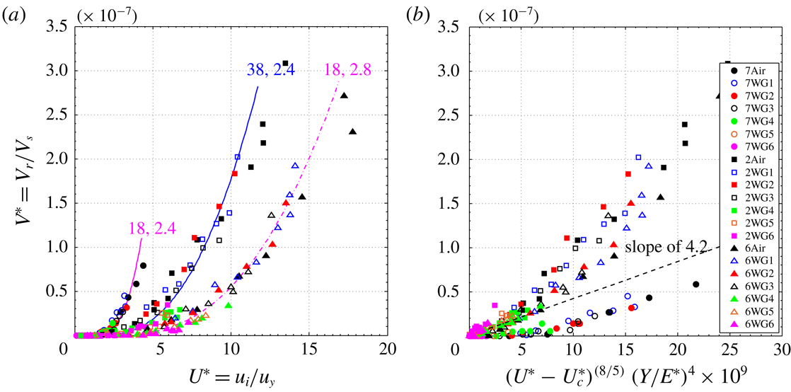
(a) Crater volume normalized by the particle volume versus the normalized velocity,
 $U^{\ast }$
. Coloured curves correspond to the model proposed by Ma & Liu (Reference Ma and Liu2015) labelled accordingly with the sets of parameters
 $\unicode[STIX]{x1D700}=\{18,28,38\}$
and
 $\unicode[STIX]{x1D713}=\{1.75,2.4\}$
shown in the legend. (b) Normalized crater volume versus reduced velocity (using
 $St_{c}=18$
) raised to the
 $8/5$
power multiplied by
 $(Y/E^{\ast })^{4}$
as suggested by (4.6). Note: in the legend, alloys are represented by the first number in their names: 7 for 7075, 2 for 2024 and 6 for 6061.

Figure 9(a) presents the normalized crater volume as a function of
 $U^{\ast }$
. Here, the normalized volume is written as,
 $V^{\ast }=V_{r}/V_{s}=(3A/8)(\unicode[STIX]{x1D6FF}_{r}/R)^{2}$
, which uses the results of figure 5,
 $R\unicode[STIX]{x1D6FF}_{r}=Aa_{r}^{2}$
and the value of
 $A$
taken from the experimental measurements. The elastic–plastic model developed by Ma & Liu (Reference Ma and Liu2015) is used to compute
 $(\unicode[STIX]{x1D6FF}_{r}/R)^{2}$
using the model parameters that fit best to the experimental data and shown on the curves. Using this approach, the predicted scaled volumes correspond to the experimental measurements.
Figure 9(b) presents the normalized crater volumes,
 $V^{\ast }$
in terms of
 $(U^{\ast }-U_{c}^{\ast })^{8/5}\times (Y/E^{\ast })^{4}\times 10^{9}$
. This scaling comes from using
 $V_{r}/V_{s}=3\unicode[STIX]{x1D6FF}_{r}a_{r}^{2}/(8R^{3})$
, substituting
 $\unicode[STIX]{x1D6FF}_{r}=A{a_{r}}^{2}/R$
, writing
 $V^{\ast }=(3A/8)\times (a_{r}/R)^{4}$
, taking
 $a_{r}/a_{y}={U^{\ast }}^{2/5}$
as suggested by the elastic scaling in (2.6a
), and
 $a_{y}/R$
from (2.5a
). Hence,
 $$\begin{eqnarray}\frac{\displaystyle V_{r}}{\displaystyle V_{s}}\approx \frac{\displaystyle 3A}{\displaystyle 8}\left(\frac{\displaystyle a_{r}}{\displaystyle R}\right)^{4}=\frac{\displaystyle 3A}{\displaystyle 8}\left(\frac{\displaystyle C_{y}\unicode[STIX]{x03C0}}{\displaystyle 2}\frac{\displaystyle Y}{\displaystyle E^{\ast }}\right)^{4}U^{\ast 8/5}=16.9A\left(\frac{\displaystyle Y}{\displaystyle E^{\ast }}\right)^{4}U^{\ast 8/5}.\end{eqnarray}$$
As noted earlier, the value of
 $A$
is
 $1/10$
for the 7075 alloy,
 $1/5$
for the 6061 alloy and
 $1/3.7$
for the 2024 alloy; over all of the materials
 $A\approx 1/4$
. If
 $U^{\ast }$
is replaced by
 $U^{\ast }-{U_{c}}^{\ast }$
, the normalized residual volume can be estimated in terms of
 $U^{\ast }$
or in terms of
 $St$
,
 $$\begin{eqnarray}\frac{\displaystyle V_{r}}{\displaystyle V_{s}}=4.2\left(\frac{\displaystyle Y}{\displaystyle E^{\ast }}\right)^{4}(U^{\ast }-{U_{c}}^{\ast })^{8/5}=4.2\left(\frac{\displaystyle Y}{\displaystyle E^{\ast }}\right)^{4}\left(\frac{\displaystyle St-St_{c}}{\displaystyle St_{y}}\right)^{8/5}.\end{eqnarray}$$
This expression is plotted in figure 9(b) and shows a reasonable correspondence with the experimental data. As noted earlier, the variation in the value of
 $A$
for the different alloys may be due to the work hardening or dynamic loading of the material. In addition, the expressions above assume a constant value for
 $C_{y}$
. Prior studies, including the original work by Bitter (Reference Bitter1963a
,Reference Bitter
b
), have suggested that the yield stress may depend on additional parameters and may differ between dynamic and static tests. Hence, it may be possible to improve the predictions by providing a better understanding of dynamic elastic–plastic transition.
5 Conclusions
The experimental measurements, reported in this article, demonstrate the importance of three non-dimensional parameters, the velocity ratio,
 $U^{\ast }=u_{i}/u_{y}$
, the Stokes number based on the yield velocity,
 $St_{y}$
, and the critical Stokes number,
 $St_{c}$
, in determining the mechanics of particle–wall collisions in a fluid. Note that the impact Stokes number can be calculated as,
 $St=U^{\ast }St_{y}$
. Most prior studies involving particle–wall collisions in a liquid have involved cases in which there is negligible plastic deformation,
 $U^{\ast }<1$
. Those studies showed that the coefficient of restitution increases from 0 at
 $St_{c}$
to a value close to one as
 $St$
approaches 1000. For cases in which
 $U\ast >1$
, an energy balance that assumes that the plastic deformation is instantaneous predicts that the coefficient of restitution reaches a maximum at an intermediate Stokes number because the plastic losses increase as
 $U^{\ast }$
and
 $St$
increase. This maximum can be estimated algebraically as a function of
 $U^{\ast }$
. The results agree reasonably well with the experimental measurements.
In terms of the crater dimensions, the surrounding fluid does not have a significant effect, except for collisions in which the Stokes number is close to the critical Stokes number. The results show that craters occur when
 $St-St_{c}>2St_{y}$
. For these conditions, the impacting particle has sufficient kinetic energy to overcome viscous losses and cause permanent damage to the target surface. For
 $St-St_{c}<2St_{y}$
, the impact does not cause damage but it may have enough kinetic energy to rebound from the surface. If the Stokes number is less than
 $St_{c}$
, the particle does not rebound from the surface. In the current experiments, the value of
 $St_{c}$
is taken as 18; however, there may be some variation between alloys.
The experimental results are also useful in developing an understanding of the surface deformation that occurs when a hard sphere collides with a softer wall in air or in a liquid. An expression is developed analytically to predict the dimensionless crater volume,
 $V^{\ast }$
, as a function of
 $St$
,
 $St_{c}$
and the material properties; the analytic expressions developed from elastic and plastic theories provide similar expressions in terms of
 $U^{\ast }$
and
 $Y/E^{\ast }$
. In the current experiments, most of the collisions are beyond the elastic regime and into the elastic–plastic regime, which was modelled using the work of Ma & Liu (Reference Ma and Liu2015). This model depends on two parameters to transition between the regimes, which are fit to the experimental data. The parameters fit to the rebound velocity did not adequately capture the data for the crater dimensions. These results suggest the need for more efforts in modelling dynamic elasto–plastic impacts. As a note, the current experiments involve ductile materials; as a result, the analysis is not directly applicable to brittle materials, such as rocks or glasses. However, the methodology presented here could be extended to these other materials, provided that there is a suitable method to model the impact behaviour of the material. Future experiments should include oblique collisions.
Acknowledgements
This research has been supported by the ACS Petroleum Research Fund through 44857-AC 9 and the National Science Foundation through grant 1706166. We also acknowledge the support of Professors G. Ravichandran and Y. C. Tai for the use of their facilities.
Appendix A
The extended derivation for the proposed formulation by Ma & Liu (Reference Ma and Liu2015) is presented in this section. The mixed elastic–plastic regime is the one that governs most of our experiments. The corresponding force-indentation constitutive relation valid for
 $\unicode[STIX]{x1D6FF}_{y}\leqslant \unicode[STIX]{x1D6FF}\leqslant \unicode[STIX]{x1D6FF}_{p}$
can be expressed as
 $$\begin{eqnarray}F_{m}=\unicode[STIX]{x1D6FF}\left[c_{1}+c_{2}\ln \left(\frac{\displaystyle \unicode[STIX]{x1D6FF}}{\displaystyle \unicode[STIX]{x1D6FF}_{y}}\right)\right]+c_{3},\end{eqnarray}$$
where
 $c_{1}$
,
 $c_{2}$
and
 $c_{3}$
are constants to be determined. The major assumption from this theory relies on the
 $C^{1}$
continuity providing four conditions to determine the interval. For both the lower bound
 $\unicode[STIX]{x1D6FF}=\unicode[STIX]{x1D6FF}_{y}$
(yield point) and the upper bound
 $\unicode[STIX]{x1D6FF}=\unicode[STIX]{x1D6FF}_{p}$
(the onset of plastic deformations) of the mixed regime, the corresponding forces (
 $F_{y}$
and
 $F_{p}$
) and the slope of the force-deflection curves (
 $F_{y}^{\prime }$
and
 $F_{p}^{\prime }$
) must match. By combining with (A 1) and the relations
 $a_{p}=\unicode[STIX]{x1D700}a_{y}$
and
 $\unicode[STIX]{x1D6FF}_{p}=a_{p}^{2}/(2R)$
, relations for the forces and the derivatives of the forces can be written as follows:
 $$\begin{eqnarray}\displaystyle \left.\begin{array}{@{}c@{}}\displaystyle F_{y}={\textstyle \frac{4}{3}}E^{\ast }R^{1/2}\unicode[STIX]{x1D6FF}_{y}^{3/2}=c_{1}\unicode[STIX]{x1D6FF}_{y}+c_{3},\\ \displaystyle F_{y}^{\prime }=\frac{\displaystyle \text{d}F_{y}}{\displaystyle \text{d}\unicode[STIX]{x1D6FF}}=2E^{\ast }\unicode[STIX]{x1D6FF}_{y}^{1/2}R^{1/2}=c_{1}+c_{2},\\ \displaystyle F_{p}=\unicode[STIX]{x1D6FF}_{p}\left[c_{1}+c_{2}\ln \left(\frac{\displaystyle \unicode[STIX]{x1D6FF}_{p}}{\displaystyle \unicode[STIX]{x1D6FF}_{y}}\right)\right]+c_{3}=\frac{\displaystyle \unicode[STIX]{x1D700}^{2}\unicode[STIX]{x1D6FF}_{y}}{\displaystyle 2}\left[c_{1}+c_{2}\ln \left(\frac{\displaystyle \unicode[STIX]{x1D700}^{2}}{\displaystyle 2}\right)\right]+c_{3},\\ \displaystyle F_{p}^{\prime }=\frac{\text{d}F_{p}}{\text{d}\unicode[STIX]{x1D6FF}}=2\unicode[STIX]{x03C0}RP_{p}=2\unicode[STIX]{x03C0}R\unicode[STIX]{x1D713}Y=c_{1}+c_{2}\!\left[\ln \!\left(\frac{\unicode[STIX]{x1D6FF}_{p}}{\unicode[STIX]{x1D6FF}_{y}}\right)+1\right]=c_{1}+c_{2}\!\left[\ln \left(\frac{\unicode[STIX]{x1D700}^{2}}{2}\right)+1\right].\end{array}\right\} & & \displaystyle \nonumber\\ \displaystyle & & \displaystyle\end{eqnarray}$$
The derivatives from the set of equations (A 2) could be set as
 $F_{y}^{\prime }=\unicode[STIX]{x03C0}R\unicode[STIX]{x1D70E}_{el}=\unicode[STIX]{x03C0}RC_{y}Y$
and
 $F_{p}^{\prime }=2\unicode[STIX]{x03C0}RP_{d}=2\unicode[STIX]{x03C0}R\unicode[STIX]{x1D713}Y$
. Then the coefficients become
 $$\begin{eqnarray}\displaystyle \left.\begin{array}{@{}c@{}}\displaystyle c_{2}=\frac{\displaystyle F_{p}^{\prime }-F_{y}^{\prime }}{\displaystyle \ln \left(\frac{\displaystyle \unicode[STIX]{x1D700}^{2}}{\displaystyle 2}\right)}=\frac{\displaystyle \unicode[STIX]{x03C0}RY(2\unicode[STIX]{x1D713}-C_{y})}{\displaystyle \ln \left(\frac{\displaystyle \unicode[STIX]{x1D700}^{2}}{\displaystyle 2}\right)},\\ \displaystyle c_{1}=F_{y}^{\prime }-c_{2},\\ \displaystyle c_{3}=F_{y}-c_{1}\unicode[STIX]{x1D6FF}_{y}.\end{array}\right\} & & \displaystyle\end{eqnarray}$$
This method differs from that elaborated by Stronge (Reference Stronge2000) by allowing the onset of plasticity to be set by the choices of
 $\unicode[STIX]{x1D700}$
and
 $\unicode[STIX]{x1D713}$
. The analysis by Stronge fixed the conditions for plastic collision. The Ma and Liu method enables the determination of the force-indentation curve and predictions of the residual crater diameter and depth along with the coefficient of restitution (COR) for any value of
 $\unicode[STIX]{x1D700}$
and
 $\unicode[STIX]{x1D713}$
. The COR then could be obtained for the three different regimes. The work presented in this manuscript is mainly associated with the mixed elastic–plastic regime, for which the compression work based on Ma & Liu (Reference Ma and Liu2015) can be written as
 $$\begin{eqnarray}W_{c}=W_{y}+\left(\frac{\displaystyle c_{1}}{\displaystyle 2}-\frac{\displaystyle c_{2}}{\displaystyle 4}\right)(\unicode[STIX]{x1D6FF}^{2}-\unicode[STIX]{x1D6FF}_{y}^{2})+\frac{\displaystyle c_{2}}{\displaystyle 2}\unicode[STIX]{x1D6FF}^{2}\ln \left(\frac{\displaystyle \unicode[STIX]{x1D6FF}}{\displaystyle \unicode[STIX]{x1D6FF}_{y}}\right)+c_{3}(\unicode[STIX]{x1D6FF}-\unicode[STIX]{x1D6FF}_{y}).\end{eqnarray}$$
The compression work is equivalent to the contact force at the end of the loading phase:
 $W_{c}=1/2mu_{i}^{2}$
. For the restitution work, Ma & Liu (Reference Ma and Liu2015) suggest
 $$\begin{eqnarray}W_{u}={\textstyle \frac{8}{15}}E^{\ast }R^{1/2}(\unicode[STIX]{x1D6FF}-\unicode[STIX]{x1D6FF}_{r})^{5/2}.\end{eqnarray}$$
Finally, for the elastic–plastic regime, the coefficient of restitution could be estimated as a function of the compression and restitution phases:
 $$\begin{eqnarray}e=\displaystyle \sqrt{\frac{W_{u}}{W_{c}}}=\sqrt{\frac{2W_{u}}{mu_{i}^{2}}}.\end{eqnarray}$$
The impact and rebound velocities and the diameter and depth of craters measured in this study can be found at https://doi.org/10.22002/D1.1151.