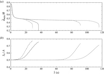
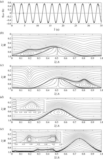
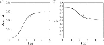
1. Introduction
Axisymmetric two-phase flows within a narrow cylindrical tube of radius
 $R$
and length
 ${\it\Lambda}$
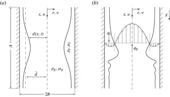
: (a) gravity-free liquid film; (b) gravity-driven liquid film. The subscript
 $g$
refers to the active core phase,
 $d(x,t)$
and
 $\bar{d}$
denote the local instantaneous and mean core radius, while
 $q_{j}$
,
 ${\it\mu}_{j}$
, and
 ${\it\rho}_{j}$
designate the flow rate, dynamic viscosity and density of the respective phases. The core flow can be quiescent, co- or countercurrent in both cases (a,b). Although our model is derived for the most general case in § 2, we apply it only to the gravity-free scenario (a) in this paper (§ 3).

The axisymmetric flow of an annular liquid film/fluid core within a cylindrical tube, as shown in figure 1, can be viewed in different limits. In the simplest case, figure 1(a), the two-phase configuration is not subjected to gravity, which can be achieved either in a microgravity environment or in a very narrow tube. If, in addition, the core phase is quiescent, the film remains ‘static’ in a noise-free environment, but is unstable to long-wave disturbances due to the Plateau–Rayleigh instability (Rayleigh Reference Rayleigh1892; Goren Reference Goren1962), with a dimensionless cutoff wavenumber
 ${\it\alpha}=2{\rm\pi}\bar{d}/{\it\Lambda}=1$
(where
 ${\it\Lambda}$
is the wavelength and
 $\bar{d}$
designates the mean core radius, which is exceptionally dimensional here). Beyond this threshold, the nonlinear evolution of a single-wavelength perturbation leads to one of two final static configurations, depending on the volume contained in the liquid film (Everett & Haynes Reference Everett and Haynes1972): an unduloid for small liquid volumes or a liquid bridge for large ones. In long tubes, where multiple unduloids may form, more complicated dynamics occurs due to interactions between large-amplitude collars and small-amplitude lobes, and the film may take a very long time to reach a final state (Lister et al.
Reference Lister, Rallison, King, Cummings and Jensen2006). The presence of an oscillating core flow can also have an effect as it may be tuned to prevent the formation of liquid bridges (Halpern & Grotberg Reference Halpern and Grotberg2003), occurring when liquid collars grow sufficiently large to occlude the tube cross-section. Prediction of this dynamics with sufficient accuracy at a reasonable computational cost is relevant for two applications: two-phase flow in porous media (Olbricht Reference Olbricht1996), encountered in the process of oil recovery by water injection, and biological films in human pulmonary capillaries and their interaction with the respiratory air flow (Grotberg Reference Grotberg1994, Reference Grotberg2011; Heil & Hazel Reference Heil and Hazel2011).
When axial gravity is added as an external driving force, figure 1(b), the film falls downward and develops long surface waves due to the convective Kapitza instability (Kapitza Reference Kapitza1948; Brooke Benjamin Reference Brooke Benjamin1957), which has been studied extensively with respect to planar falling liquid films (Alekseenko, Nakoryakov & Pokusaev Reference Alekseenko, Nakoryakov and Pokusaev1994; Kalliadasis et al. Reference Kalliadasis, Ruyer-Quil, Scheid and Velarde2012). In our cylindrical case, this dynamics is modified by the Plateau–Rayleigh instability due to azimuthal free-surface curvature (Ruyer-Quil et al. Reference Ruyer-Quil, Trevelyan, Giorgiutti-Dauphine, Duprat and Kalliadasis2008). This introduces the possibility of absolute instability, i.e. temporal growth of localized disturbances, which may explain the occlusion of narrow tubes by wavy falling films (Trifonov Reference Trifonov1992; Dao & Balakotaiah Reference Dao and Balakotaiah2000). Further, the presence of a core (co- or countercurrent) gas flow may alter the dynamics leading to this flooded state, as has been established for planar films in narrow channels (Drosos, Paras & Karabelas Reference Drosos, Paras and Karabelas2006; Trifonov Reference Trifonov2010a ,Reference Trifonov b ; Dietze & Ruyer-Quil Reference Dietze and Ruyer-Quil2013). Prediction and prevention of flooding is crucial for the efficient design and operation of tubular falling film evaporators used, e.g., for milk inspissation (Jebson & Chen Reference Jebson and Chen1997).
When the main driving force results from an imposed pressure difference, one obtains what is conventionally referred to as core–annular flow (Joseph, Chen & Renardy Reference Joseph, Chen and Renardy1997), where both phases are usually cocurrent (technically, figures 1(a,b) also depict core–annular flows). Such flows may occur in lubricated pipelining (Aul & Olbricht Reference Aul and Olbricht1990; Joseph et al. Reference Joseph, Bai, Mata, Sury and Grant1999; Gosh et al. Reference Gosh, Mandal, Das and Das2009) or in human bronchial airways (Camassa et al. Reference Camassa, Forest, Lee, Ogrosky and Olander2012). They are more complicated than the first two scenarios as interfacial waves can result from two additional instabilities: the long-wave Yih instability due to viscosity stratification (Yih Reference Yih1967; Hickox Reference Hickox1971) and a short-wave instability of the Tollmien–Schlichting type (Hu & Joseph Reference Hu and Joseph1989; Preziosi, Chen & Joseph Reference Preziosi, Chen and Joseph1989). Moreover, an absolute instability can occur even in the absence of surface tension, e.g. in miscible liquid/liquid systems (d’Olce et al. Reference d’Olce, Martin, Rakotomalala, Salin and Talon2008, Reference d’Olce, Martin, Rakotomalala, Salin and Talon2009; Selvam et al. Reference Selvam, Talon, Lesshafft and Meiburg2009). These instability mechanisms lead to nonlinear interfacial deformations that significantly alter the flow field (Newhouse & Pozrikidis Reference Newhouse and Pozrikidis1992; Bai, Kelkar & Joseph Reference Bai, Kelkar and Joseph1996; Kouris & Tsamopoulos Reference Kouris and Tsamopoulos2001, Reference Kouris and Tsamopoulos2002; Govindarajan & Sahu Reference Govindarajan and Sahu2014).
In this paper, we introduce a low-dimensional model based on the weighted residual integral boundary layer (WRIBL) method (Ruyer-Quil & Manneville Reference Ruyer-Quil and Manneville2002; Kalliadasis et al. Reference Kalliadasis, Ruyer-Quil, Scheid and Velarde2012) that is capable of accurately predicting the linear and nonlinear dynamics of the three above-discussed long-wave instability mechanisms at low computational cost. We derive this model for the most general case (figure 1), ensuring applicability for all three flow scenarios, yet apply it only to the first scenario, i.e. gravity-free liquid films in interaction with an active fluid core, figure 1(a), leaving investigation of the other scenarios for future work. For reasons that are obvious for applications involving such flows, particular attention is paid to the phenomenon of flooding, when interfacial deformations become so large that they form a liquid bridge occluding the cross-section of the tube.
We proceed next with an account of previous modelling work, before discussing the salient/novel features of our model. Regarding the gravity-free configuration in figure 1(a), early modelling works considered only the liquid film, assuming a passive core fluid, which is valid, e.g., for liquid/gas configurations or liquid/liquid configurations dominated by viscous forces (when the film is significantly more viscous than the core). In this limit, Hammond (Reference Hammond1983) derived an evolution equation for the core radius
 $d$
by applying lubrication theory. This amounts to imposing a locally developed flow at all times and thus neglecting inertia and streamwise viscous diffusion altogether. Additionally, Hammond made the assumption of thin films, i.e.
 $(R-\bar{d})\ll R$
(where
 $\bar{d}$
once again is dimensional). The resulting evolution equation enabled first calculations of nonlinear interfacial deformations, showing the liquid film to organize into ring-shaped collars separated by thin residual film portions or lobes. However, these calculations could not yield insight into the dynamics once the liquid film grows locally thick whilst the lobes drain into the collars. Nonetheless, calculations on long domains by Lister et al. (Reference Lister, Rallison, King, Cummings and Jensen2006), using the same evolution equation, showed that intricate interactions between several neighbouring lobes and collars occur before that limit is reached and drastically slow the drainage of the liquid film. Viscous dissipation in the very thin lobes is decisive for this behaviour, an observation that we will revisit in § 3.3. By relaxing the thin-film hypothesis in the formulation of the interfacial pressure jump, Gauglitz (Reference Gauglitz1988) obtained an evolution equation that can extend beyond thin films and in principle produce the large-amplitude equilibrium shapes of this problem, i.e. stable unduloids and liquid bridges.
A first attempt to account for the effect of an active core fluid was made by Halpern & Grotberg (Reference Halpern and Grotberg2003). Their approach represents the liquid film with a similar evolution equation to Gauglitz (Reference Gauglitz1988), while taking into account the tangential stress and axial pressure gradient exerted at the fluid/fluid interface by the core fluid. These coupling quantities are obtained by solving the core flow under the assumption of a ‘frozen’ film surface. This is valid in the limit of high-frequency core-flow oscillations considered by Halpern & Grotberg (Reference Halpern and Grotberg2003) as a means to prevent flooding. Comparison with experiments and direct numerical simulations (DNS) was subsequently performed in the passive-core limit (Bian et al. Reference Bian, Tai, Halpern, Zheng and Grotberg2010; Tai et al. Reference Tai, Bian, Halpern, Zheng, Filoche and Grotberg2011). We also note that Halpern, Fujioka & Grotberg (Reference Halpern, Fujioka and Grotberg2010) introduced a passive-core lubrication model for viscoelastic liquid films. Elsewhere, modelling has been undertaken to study the pinch-off of a slender cylindrical fluid thread surrounded by a second fluid phase. Such works usually assume inertialess flow (Sierou & Lister Reference Sierou and Lister2003) and are obtained by long-wave asymptotic expansion.
A shortcoming of the above-described modelling approaches is that they do not account for inertia, which limits their applicability to viscosity-dominated flows. For the case of a passive core, Johnson et al. (Reference Johnson, Kamm, Ho, Shapiro and Pedley1991) remedied this using an integral approach, without additionally assuming thin films. By radially integrating the continuity and first-order long-wave Navier–Stokes equations (prescribing an inviscid velocity profile for inertial terms and an inertialess profile for viscous terms) across the liquid film, a two-equation model was obtained. Comparisons with exact linear stability calculations showed good agreement in the inviscid and inertialess limits, and less good agreement when both inertia and viscosity are relevant. For the case of a mucus-film/passive-core configuration, the model was shown to capture the formation of unduloids and liquid bridges in accordance with the criterion of Everett & Haynes (Reference Everett and Haynes1972). We note that some works on modelling the pinch-off of slender fluid threads have also accounted for (weak) inertia (Eggers & Dupont Reference Eggers and Dupont1994; Eggers & Villermaux Reference Eggers and Villermaux2008; Wang Reference Wang2013).
Regarding gravity-driven liquid-film/core-fluid configurations, modelling work has primarily focused on a passive core fluid. Trifonov (Reference Trifonov1992) applied the (first-order) long-wave integral boundary layer (IBL) method of Shkadov (Reference Shkadov1967) to falling films flowing within cylindrical tubes (and on cylindrical wires). Another approach was applied by Jensen (Reference Jensen2000), who derived evolution equations for different portions of the wavy liquid film. Modelling work accounting for an active core fluid (to the best of our knowledge) has been very scarce. Only recently, Mehidi & Amatousse (Reference Mehidi and Amatousse2009) derived a fully coupled liquid-film/core-fluid model by applying the WRIBL approach to the case of exclusively gravity-driven core–annular flow, i.e. in the absence of any axial pressure difference. However, this work was limited to linear stability calculations. We also note that a number of works have focused on the related situation of a liquid film flowing down a cylindrical fibre in a passive atmosphere (Quéré Reference Quéré1999). For instance, Novbari & Oron (Reference Novbari and Oron2009, Reference Novbari and Oron2011) used the energy integral method (EIM), akin to the WRIBL method, to derive a first-order model. Later, Ruyer-Quil et al. (Reference Ruyer-Quil, Trevelyan, Giorgiutti-Dauphine, Duprat and Kalliadasis2008) and Ruyer-Quil & Kalliadasis (Reference Ruyer-Quil and Kalliadasis2012) obtained a second-order WRIBL model and showed that accounting for streamwise viscous diffusion significantly improves linear and nonlinear predictions. We also note the work of Wray (Reference Wray2013), who derived a thin-film model for electrolyte films in annular gaps.
Regarding pressure-driven core–annular flow, we only briefly mention three modelling works dealing with thin films, referring the reader to Chen & Joseph (Reference Chen and Joseph1991) for more information. Frenkel et al. (Reference Frenkel, Babchin, Levich, Shlang and Sivashinsky1987) derived a lubrication model for the case of equal densities and viscosities and showed that the presence of a mean flow could saturate interfacial waves resulting from the Plateau–Rayleigh instability. Similarly, Papageorgiou, Maldarelli & Rumschitzki (Reference Papageorgiou, Maldarelli and Rumschitzki1990) derived a weakly nonlinear model that allows for disparate viscosities in the film and core. Later, Kerchman (Reference Kerchman1995) derived a thin-film evolution equation by asymptotic expansion, while taking into account the interfacial shear stress exerted on the liquid film by the core flow. Nonlinear simulations using this model were shown to be in good agreement with experiments by Aul & Olbricht (Reference Aul and Olbricht1990).
The model introduced in this paper mitigates some of the above-discussed shortcomings of previous modelling works. It is obtained by applying the WRIBL approach to both fluid phases, while fully taking into account interphase coupling. In that sense, it is a cylindrical extension of the planar two-phase model of Dietze & Ruyer-Quil (Reference Dietze and Ruyer-Quil2013). The underlying assumptions are that interfacial deformations remain long compared with the radial extent of the respective phases, which we express in terms of the long-wave parameter
 ${\it\epsilon}=R/{\it\Lambda}\ll 1$
, that the characteristic Reynolds number is moderate in both phases (inertial effects are moderate) and that the Weber number, relating inertia to capillary forces, is small (capillary effects are important). Our model is based on a second-order development in the long-wave parameter
 ${\it\epsilon}$
so that inertia, streamwise viscous diffusion and viscous stresses in the interphase coupling conditions are taken into account.
In particular, this leads to the following salient/novel features. (a) By design, the model analytically yields the asymptotic growth rates and wave speeds of long-wave instabilities in core–annular flow (Hickox Reference Hickox1971). Further, the short-wave linear cutoff wavelength for the gravity-free scenario (Plateau–Rayleigh instability) is recovered analytically. (b) By accounting for inertia, the model allows us to treat situations that do not satisfy the creeping-flow assumption. For example, we show in § 3.1 that this is the case for liquid-bridge formation in a gravity-free water/air system. In contrast to lubrication theory models, our model can accurately predict the time to flooding even in such situations. Further, the WRIBL approach applies a consistent base velocity profile when integrating the boundary layer equations, as opposed to Johnson et al. (Reference Johnson, Kamm, Ho, Shapiro and Pedley1991), who used different approximations (inviscid, inertialess) for different terms in the governing equations (inertial, viscous). This improves the consistency of linear instability predictions when inertial and viscous effects are relevant. We also point out that accounting for inertia is a basic requirement to capture surface waves in falling liquid films. (c) The model treats both phases equally and fully accounts for interphase coupling, without imposing any restrictions on the fluid combination. As opposed to passive core models (Johnson et al. Reference Johnson, Kamm, Ho, Shapiro and Pedley1991; Trifonov Reference Trifonov1992), it can thus treat fluid combinations where the film viscosity is not dominant, e.g. water/silicone oil. Further, it allows us to fully reconstruct the velocity field in both phases and is not limited to high-frequency core-flow oscillations, as opposed to the model by Halpern & Grotberg (Reference Halpern and Grotberg2003). (d) Our model includes an additional equation for the axial derivative of the interfacial core-fluid pressure, enabling us to predict the pressure drop in the case of imposed flow rate or to impose a driving pressure difference. This allows us to consider different types of driving force. In particular, the three scenarios encompassed by figure 1 can be recovered, i.e. gravity-free and gravity-driven liquid films in interaction with an active co- or countercurrent core flow and pressure-driven core–annular flows. By contrast, Mehidi & Amatousse (Reference Mehidi and Amatousse2009) assume a zero pressure drop in their model, which is thus limited to exclusively gravity-driven cocurrent two-phase flow. (e) Our model does not assume thin films in relation to the tube radius and can thus predict large-amplitude interfacial deformations up to the point of flooding, when the cross-section of the tube is obstructed. ( f) By accounting for streamwise viscous diffusion (in both phases), our model can accurately predict the dynamics of very thin films developing capillary waves or bulges. For example, we show in § 3.3 that this is essential to accurately capture the long-time behaviour of thin gravity-free films. Also, it is essential to describe capillary waves in falling liquid films. (g) Finally, our model allows calculations at drastically reduced computational cost in comparison to full DNS.
The remainder of the paper is structured as follows. We derive our WRIBL model from first principles in § 2 for the most general case (figure 1), i.e. without distinguishing between the scenarios of gravity-free/gravity-driven films and pressure-driven core–annular flows. Therein, specific care is taken to write mathematical expressions in a succinct form, in order to allow reuse of the model by others. In § 3, we apply our model to gravity-free liquid films in interaction with an active fluid core, figure 1(a).
Specific attention is paid to the phenomenon of flooding, which occurs when liquid collars grow sufficiently large to form a liquid bridge occluding the tube cross-section. We start in § 3.1 by validating model calculations with Navier–Stokes calculations of linear stability and nonlinear two-phase flow dynamics. In §§ 3.2–3.4, we then focus on a number of novel/salient features which we have found for this declaredly well studied flow scenario thanks to the advantages/improvements contained in our model. First (§ 3.2), we have found that accounting for inertia as well as full coupling between the liquid film and the fluid core is essential to accurately predict the flooding dynamics for fluid pairings that are not dominated by viscosity, e.g. water/air and water/silicone oil. Second, § 3.3 concerns an interesting phenomenon we have observed in liquid films that are rather thin, yet too thick to develop an unduloid and must thus eventually evolve towards a liquid bridge. We have found that this transition is drastically slowed and effectively halted due to a viscous-blocking mechanism that intervenes once the thin residual film between two liquid collars has buckled. Only at very large times does flooding eventually occur, when symmetry breaking in the buckled residual film (due to small perturbations) produces a sliding motion that reinitiates growth of the liquid collars. Importantly, streamwise viscous diffusion is essential to accurately predict this mechanism. Finally, § 3.4 investigates the effect of a low-frequency oscillating core flow, such as may occur in human pulmonary capillaries. Interestingly, we find that such oscillations accelerate the above-described sliding-induced flooding mechanism. In §§ 3.3 and 3.4, we also show the occurrence of intricate vorticity-carrying structures in the two-phase flow. Conclusions are drawn in § 4 and the paper is completed by appendices succinctly summarizing mathematical expressions intervening in § 2 (appendices A–C) and presenting supplementary validation results (appendix D).
2. Model formulation
We consider the laminar axisymmetric flow of two immiscible continuous and constant-property Newtonian fluid phases within a cylindrical tube, as sketched in figure 1. The inner phase of this core–annular flow arrangement is referred to with subscript ‘
 $g$
’, while the phase lining the tube wall is indexed with ‘
 $l$
’. In subsequent sections, we will consider a specific subscenario, i.e. gravity-free liquid films subjected to an active gas or liquid core, where the relative orientation of the flow rates
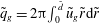 $\tilde{q}_{g}=2{\rm\pi}\!\int _{0}^{\tilde{d}}\tilde{u} _{g}\tilde{r}\text{d}\tilde{r}$
and
 $\tilde{q}_{l}=2{\rm\pi}\!\int _{\tilde{d}}^{R}\tilde{u} _{l}\tilde{r}\text{d}\tilde{r}$
varies. In the current section, we make assumptions neither about this nor about the nature of the driving force and consider the most general case. We also note that the tilde symbol is used to distinguish dimensional quantities throughout.
2.1. Governing equations truncated in the long-wave limit
Our study is focused on wavy core–annular flows displaying wavelengths much larger than the radius of the tube, i.e.
 ${\it\epsilon}=R/{\it\Lambda}\ll 1$
. We invoke this long-wave assumption to truncate the governing equations at
 $O({\it\epsilon}^{2})$
, following Dietze & Ruyer-Quil (Reference Dietze and Ruyer-Quil2013), who derived a similar model for two-phase flow through a rectangular channel. From the axial and radial Navier–Stokes equations, one thus obtains the
 $O({\it\epsilon}^{2})$
-consistent boundary layer equations for the respective phases, written here in non-dimensional notation (
 $j=l,g$
):
 $$\begin{eqnarray}\mathit{Re}_{j}\left[\partial _{t}u_{j}+u_{j}\partial _{x}u_{j}+v_{j}\partial _{r}u_{j}\right]=-\mathit{Re}_{j}\partial _{x}\left(p_{j}|_{r=d}\right)+\frac{\mathit{Re}_{j}}{\mathit{Fr}^{2}}+\mathscr{L}(u_{j})+2\partial _{xx}u_{j}-\partial _{x}(\partial _{x}u_{j}|_{r=d}),\end{eqnarray}$$
where lengths have been non-dimensionalized with the tube radius
 $R$
, velocities with a characteristic velocity
 $U$
, pressure with the corresponding dynamic pressure
 ${\it\rho}_{j}U^{2}$
and time using
 $R/U$
. Non-dimensional variables are denoted using regular symbols, i.e. without any attributes, as opposed to dimensional quantities which will be distinguished with a tilde. The dimensionless groups appearing in the above equations are the Reynolds numbers
 $\mathit{Re}_{j}=UR{\it\rho}_{j}/{\it\mu}_{j}$
and the Froude number
 $\mathit{Fr}=U/(gR)^{1/2}$
. We note that the same velocity scale
 $U$
is chosen for both phases in order to ensure consistent time scales. If the flow rates in the annular and/or core phase are imposed,
 $U$
may be chosen as one of the superficial velocities, while, in the case of a static film/core arrangement, an internal velocity scale such as that obtained by balancing capillary and viscous forces, i.e.
 $U={\it\sigma}/{\it\mu}_{l}$
, may be chosen. In (2.1a
),
 $\mathscr{L}$
refers to the Laplacian radial operator in axisymmetric geometries, i.e.
 $\mathscr{L}({\it\phi})\equiv (1/r)(\partial /\partial r)(r(\partial {\it\phi}/\partial r))$
. In (2.1a
), the free-surface terms
 $\partial _{x}(p_{j}|_{r=d})$
and
 $\partial _{x}(\partial _{x}u_{j}|_{r=d})$
were substituted for the pressure derivative
 $\partial _{x}p_{j}$
in the axial momentum equation as a result of integrating the radial momentum equation from
 $r$
to
 $d$
. Meanwhile, the continuity equation is written as
 $$\begin{eqnarray}\frac{1}{r}\frac{\partial }{\partial r}\left(rv_{j}\right)+\partial _{x}u_{j}=0.\end{eqnarray}$$
Equations (2.1a
) and (2.1b
) are completed by the
 $O({\it\epsilon}^{2})$
interphase coupling conditions for normal and tangential stresses at
 $r=d$
:
 $$\begin{eqnarray}\displaystyle \mathit{Re}_{l}\left(p_{l}-{\it\Pi}_{{\it\rho}}p_{g}\right) & = & \displaystyle \mathit{We}^{-1}\mathit{Re}_{l}{\it\kappa}+2\left[\partial _{r}v_{l}-\partial _{x}d\partial _{r}u_{l}\right]-2{\it\Pi}_{{\it\mu}}[\partial _{r}v_{g}-\partial _{x}d\partial _{r}u_{g}],\end{eqnarray}$$
 $$\begin{eqnarray}\displaystyle \partial _{r}u_{l}-{\it\Pi}_{{\it\mu}}\partial _{r}u_{g} & = & \displaystyle 2\partial _{x}d\left(\partial _{x}u_{l}-\partial _{r}v_{l}\right)-\partial _{x}v_{l}-{\it\Pi}_{{\it\mu}}\left[2\partial _{x}d\left(\partial _{x}u_{g}-\partial _{r}v_{g}\right)-\partial _{x}v_{g}\right]\!,\end{eqnarray}$$
where
 $\mathit{We}=({\it\rho}_{l}RU_{l}^{2})/{\it\sigma}$
is the Weber number (it should be noted that, in the literature on falling liquid films,
 $\mathit{We}$
is written as the inverse of this definition),
 ${\it\Pi}_{{\it\mu}}={\it\mu}_{g}/{\it\mu}_{l}$
and
 ${\it\Pi}_{{\it\rho}}={\it\rho}_{g}/{\it\rho}_{l}$
designate the viscosity and density ratios, and
 ${\it\kappa}$
represents the free-surface curvature truncated at
 $O({\it\epsilon}^{2})$
:
 $$\begin{eqnarray}{\it\kappa}=\partial _{xx}d-\frac{1}{d}\left[1-\frac{1}{2}\left(\partial _{x}d\right)^{2}\right],\end{eqnarray}$$
as well as the continuity for the velocity components:
 $$\begin{eqnarray}u_{l}|_{r=d}=u_{g}|_{r=d},\quad v_{l}|_{r=d}=v_{g}|_{r=d}.\end{eqnarray}$$
The system is completed by the no-slip condition at the tube wall and the symmetry condition at the centreline:
 $$\begin{eqnarray}u_{l}|_{r=1}=v_{l}|_{r=1}=0,\quad \partial _{r}u_{g}|_{r=0}=v_{g}|_{r=0}=0.\end{eqnarray}$$
2.2. Weighted integral approach
Following Dietze & Ruyer-Quil (Reference Dietze and Ruyer-Quil2013), we obtain our model equations by weighted integration of (2.1a
) across the respective phases. Formally, we introduce the scalar product
 $\langle A|B\rangle =2{\rm\pi}({\it\Pi}_{{\it\mu}}\int _{0}^{d}A_{g}B_{g}r\text{d}r+\int _{d}^{1}A_{l}B_{l}r\text{d}r)$
, where the choice of a factor
 ${\it\Pi}_{{\it\mu}}$
in front of the integral in the gas phase is a direct consequence of the continuity of tangential stresses (2.1d
). Writing the boundary layer equations (2.1a
) as
 $\mathit{BLE}_{j}$
, we introduce the weight functions
 $w_{j}(r)$
and evaluate the residual
 $\langle \mathit{BLE}|w\rangle$
. This will lead to two dynamic model equations derived in the following subsections. In addition, two kinematic equations are obtained by integrating (2.1b
) across the respective phases (
 $j=l,g$
):
 $$\begin{eqnarray}\partial _{x}q_{j}-{\it\varepsilon}_{j}2{\rm\pi}d\partial _{t}d=0,\end{eqnarray}$$
where the kinematic condition
 $v_{j}|_{r=d}=\partial _{t}d+u_{j}|_{r=d}\partial _{x}d$
was employed and
 ${\it\varepsilon}_{l}=1$
,
 ${\it\varepsilon}_{g}=-1$
.
2.3. Decomposition of the velocity field
To evaluate
 $\langle \mathit{BLE}|w\rangle$
, we decompose the streamwise velocity component into an
 $O(1)$
and an
 $O({\it\epsilon})$
contribution:
 $$\begin{eqnarray}u_{j}(x,r,t)=\underbrace{\hat{u} _{j}(x,r,t)}_{O(1)}+\underbrace{u_{j}^{(1)}(x,r,t)}_{O\left({\it\epsilon}\right)}.\end{eqnarray}$$
The leading-order profile
 $\hat{u} _{j}(x,r,t)$
satisfies the governing equations (2.1) truncated at
 $O(1)$
and is additionally required to yield the local and instantaneous flow rates in the respective phases, i.e.
 $$\begin{eqnarray}q_{l}=2{\rm\pi}\int _{d}^{1}\hat{u} _{l}r\text{d}r,\quad q_{g}=2{\rm\pi}\int _{0}^{d}\hat{u} _{g}r\text{d}r,\end{eqnarray}$$
which amounts to imposing a gauge condition on the
 $O({\it\epsilon})$
corrections
 $u^{(1)}$
:
 $$\begin{eqnarray}\int _{0}^{d}u_{g}^{(1)}r\text{d}r=\int _{d}^{1}u_{l}^{(1)}r\text{d}r=0.\end{eqnarray}$$
This ensures that
 $\hat{u} _{j}$
is sufficiently close to the real profile (as evidenced by the flow field comparisons in figures 4, 7
a,b) so that the separation of scales (2.3) remains satisfied. It turns out that
 $\hat{u} _{j}(x,r,t)$
can then be written as
 $$\begin{eqnarray}\hat{u} _{j}(x,r,t)=q_{i}(x,t)f_{ij}(r;d),\end{eqnarray}$$
where, once again,
 $j=l,g$
distinguishes the two phases and the explicit dependence on the core radius
 $d$
is emphasized by the notation
 $f_{ij}(r;d)$
. Also, Einstein’s notation has been used so that
 $q_{i}(x,t)f_{ij}(r;d)$
is to be read as the sum
 $q_{g}(x,t)f_{gj}(r;d)+q_{l}(x,t)f_{lj}(r;d)$
. The formulation in (2.6) will help in deriving the model equations in a succinct form. Agreement of the ansatz (2.6) with the base state requires that the functions
 $f_{ij}$
satisfy
 $$\begin{eqnarray}\mathscr{L}\left(f_{ij}\right)\equiv \frac{1}{r}\frac{\partial }{\partial r}\left(r\frac{\partial f_{ij}}{\partial r}\right)=C_{ij},\end{eqnarray}$$
with the boundary conditions
 $$\begin{eqnarray}\left.\begin{array}{@{}l@{}}f_{il}|_{r=d}=f_{ig}|_{r=d},\quad \partial _{r}f_{il}|_{r=d}={\it\Pi}_{{\it\mu}}\partial _{r}f_{ig}|_{r=d},\\ f_{il}|_{r=1}=0\quad \text{and}\quad \partial _{r}f_{ig}|_{r=0}=0.\end{array}\!\!\right\}\end{eqnarray}$$
The solutions to this boundary value problem (2.7) are as follows:
 $$\begin{eqnarray}\displaystyle \left.\begin{array}{@{}l@{}}\displaystyle f_{jl}(r;d)=\frac{C_{jl}}{4}\left(r^{2}-1\right)+D_{jl}\ln (r)\quad \text{with }D_{jl}=\frac{d^{2}}{2}\left({\it\Pi}_{{\it\mu}}C_{jg}-C_{jl}\right),\\ \displaystyle f_{jg}(r;d)=\frac{C_{jg}}{4}\left(r^{2}-d^{2}\right)+f_{jl}(d;d)\quad \text{with }f_{jl}(d;d)=\frac{1}{4}C_{jl}(d^{2}-1)+D_{jl}\ln (d),\end{array}\!\!\right\} & & \displaystyle \nonumber\\ \displaystyle & & \displaystyle\end{eqnarray}$$
wherein the constants
 $C_{ij}$
are determined by the integral constraints resulting from (2.4):
 $$\begin{eqnarray}2{\rm\pi}\int _{0}^{d}f_{ig}r\text{d}r={\it\delta}_{ig}\quad \text{and}\quad 2{\rm\pi}\int _{d}^{1}f_{il}r\text{d}r={\it\delta}_{il},\end{eqnarray}$$
and
 ${\it\delta}_{ij}$
is the usual Kronecker symbol.
The radial velocity component
 $v$
is computed from the continuity equation (2.1b
), using the no-penetration condition at the wall
 $v_{l}|_{r=1}=0$
and the symmetry condition
 $v_{g}|_{r=0}=0$
on the centreline:
 $$\begin{eqnarray}v_{g}=-\frac{1}{r}\int _{0}^{r}\partial _{x}u_{g}r\text{d}r\quad \text{and}\quad v_{l}=-\frac{1}{r}\int _{1}^{r}\partial _{x}u_{l}r\text{d}r.\end{eqnarray}$$
Later, it will become necessary to compute the derivatives of
 $\hat{u} (x,r,t)$
with respect to the core radius
 $d$
. We introduce a simplified notation for these derivatives here. The first derivatives
 $\partial _{d}\,f_{ij}=\lim _{{\it\delta}d\rightarrow 0}\{(f_{ij}(r;d+{\it\delta}d)-f_{ij}(r;d))/{\it\delta}d\}$
are solutions to
 $\mathscr{L}(\partial _{d}\,f_{ij})=\partial _{d}C_{ij}$
in addition to verifying the integral constraints
 $$\begin{eqnarray}\int _{0}^{d}\partial _{d}\,f_{ig}r\text{d}r+df_{ig}|_{r=d}=0,\quad \int _{d}^{1}\partial _{d}\,f_{il}r\text{d}r-df_{ig}|_{r=d}=0,\end{eqnarray}$$
the boundary conditions (2.7b
) derived with respect to
 $d$
and the coupling conditions at the free surface (
 $r=d$
)
 $$\begin{eqnarray}\partial _{d}\,f_{il}+\partial _{r}f_{il}=\partial _{d}\,f_{ig}+\partial _{r}f_{ig},\quad \partial _{dr}f_{il}+\partial _{rr}f_{il}={\it\Pi}_{{\it\mu}}[\partial _{dr}f_{ig}+\partial _{rr}f_{ig}].\end{eqnarray}$$
Since
 $\partial _{d}\,f_{ij}$
and
 $f_{ij}$
satisfy similar linear boundary value problems, they can be expressed as a linear combination of one another:
 $$\begin{eqnarray}\partial _{d}\,f_{ij}=a_{ijk}f_{kj},\end{eqnarray}$$
wherein the coefficients
 $a_{ijk}$
are functions of
 $f_{il}|_{r=d}$
and
 $\partial _{r}f_{il}|_{r=d}$
, exceptionally denoted
 $f_{il}$
and
 $\partial _{r}f_{il}$
here,
 $$\begin{eqnarray}\displaystyle & a_{ill}=2{\rm\pi}f_{il}d, & \displaystyle\end{eqnarray}$$
 $$\begin{eqnarray}\displaystyle & \displaystyle a_{igl}=a_{ill}+\frac{{\it\Pi}_{{\it\mu}}\,f_{gl}\left[-C_{il}+{\it\Pi}_{{\it\mu}}C_{ig}\right]+\partial _{r}f_{gl}({\it\Pi}_{{\it\mu}}-1)\partial _{r}f_{il}}{{\it\Pi}_{{\it\mu}}D}, & \displaystyle\end{eqnarray}$$
 $$\begin{eqnarray}\displaystyle & a_{igg}=-2{\rm\pi}f_{il}d, & \displaystyle\end{eqnarray}$$
 $$\begin{eqnarray}\displaystyle & \displaystyle a_{ilg}=a_{igg}+\frac{{\it\Pi}_{{\it\mu}}\,f_{ll}\left[-C_{il}+{\it\Pi}_{{\it\mu}}C_{ig}\right]+\partial _{r}f_{ll}({\it\Pi}_{{\it\mu}}-1)\partial _{r}f_{il}}{{\it\Pi}_{{\it\mu}}D}, & \displaystyle\end{eqnarray}$$
 $$\begin{eqnarray}\displaystyle & D=f_{ll}\partial _{r}f_{gl}-f_{gl}\partial _{r}f_{ll}. & \displaystyle\end{eqnarray}$$
 $$\begin{eqnarray}v_{j}=-\frac{1}{r}\left[a_{ijk}q_{i}\partial _{x}dl_{kj}(r;d)+\partial _{x}q_{i}l_{ij}(r;d)\right]+O({\it\epsilon}),\end{eqnarray}$$
where
 $$\begin{eqnarray}\displaystyle l_{ig}(r;d) & \equiv & \displaystyle \int _{0}^{r}f_{ig}r\text{d}r\nonumber\\ \displaystyle & = & \displaystyle \frac{r^{2}}{96}\left\{C_{ig}^{2}r^{4}-3C_{ig}r^{2}\left(C_{ig}d^{2}-4f_{il}(d;d)\right)+3\left(C_{ig}d^{2}-4f_{il}(d;d)\right)^{2}\right\},\nonumber\\ \displaystyle & & \displaystyle\end{eqnarray}$$
 $$\begin{eqnarray}\displaystyle l_{il}(r;d) & \equiv & \displaystyle \int _{1}^{r}f_{il}r\text{d}r\nonumber\\ \displaystyle & = & \displaystyle \frac{1}{96}\left\{(r^{2}-1^{2})\left[C_{il}^{2}(r^{2}-1^{2})^{2}-3C_{il}D_{il}(r^{2}-31^{2})+24D_{il}^{2}\right]\right.\nonumber\\ \displaystyle & & \displaystyle \left.+\,12D_{il}r^{2}\ln (r)\left[C_{il}(r^{2}-2)+4D_{il}\ln (r)\right]\right\}.\end{eqnarray}$$
 $\partial _{dd}\,f_{ij}=b_{ijk}f_{kj}$
, where the coefficients
 $b_{ijk}$
are again functions of
 $f_{il}|_{r=d}$
and
 $\partial _{r}f_{il}|_{r=d}$
, once again denoted
 $f_{il}$
and
 $\partial _{r}f_{il}$
here for simplicity:
 $$\begin{eqnarray}\displaystyle b_{ill} & = & \displaystyle -2{\rm\pi}\left[f_{il}+d\left(\partial _{d}\,f_{il}+\partial _{r}f_{il}\right)\right],\end{eqnarray}$$
 $$\begin{eqnarray}\displaystyle b_{igl} & = & \displaystyle b_{ill}+\left(Dd\right)^{-1}\left\{f_{gl}\left[-C_{il}-2d\partial _{d}C_{il}+{\it\Pi}_{{\it\mu}}C_{ig}+2{\it\Pi}_{{\it\mu}}d\partial _{d}C_{ig}\right]\right.\nonumber\\ \displaystyle & & \displaystyle \left.+\,\partial _{r}f_{gl}\left[d\left(C_{il}-C_{ig}\right)-\partial _{d}\,f_{ig}+\partial _{d}\,f_{il}+2d\left(\partial _{dr}f_{il}-\partial _{dr}f_{ig}\right)\right]\right\},\end{eqnarray}$$
 $$\begin{eqnarray}\displaystyle b_{ilg} & = & \displaystyle b_{igg}+\left(Dd\right)^{-1}\left\{f_{ll}\left[-C_{il}-2d\partial _{d}C_{il}+{\it\Pi}_{{\it\mu}}C_{ig}+2{\it\Pi}_{{\it\mu}}d\partial _{d}C_{ig}\right]\right.\nonumber\\ \displaystyle & & \displaystyle \left.+\,\partial _{r}f_{ll}\left[d\left(C_{il}-C_{ig}\right)-\partial _{d}\,f_{ig}+\partial _{d}\,f_{il}+2d\left(\partial _{dr}f_{il}-\partial _{dr}f_{ig}\right)\right]\right\},\end{eqnarray}$$
 $$\begin{eqnarray}\displaystyle b_{igg} & = & \displaystyle -2{\rm\pi}\left[f_{ig}+d\left(\partial _{d}\,f_{ig}+\partial _{r}f_{ig}\right)\right].\end{eqnarray}$$
2.4. Choice of weight functions
 $w_{j}$
and elimination of velocity corrections
$u_{j}^{(1)}$


For the much simpler case of a liquid film in a passive atmosphere, Ruyer-Quil, Kofman & Chasseur (Reference Ruyer-Quil, Kofman and Chasseur2014) showed that, by substituting (2.3) for
 $u_{j}$
in the governing equations, the correction fields
 $u_{j}^{(1)}$
could be solved recursively as a series in
 ${\it\epsilon}$
. In our case, this would have the form
 $\sum _{k}{\it\epsilon}^{k}u_{jk}^{(1)}(q_{j},d,\partial _{x}p_{j}|_{r=d},r)$
and the gauge conditions (2.5) would yield two dynamic model equations coupling the core radius, flow rates and pressure gradients (related by (2.1c
)). However, this approach would involve cumbersome algebra. The weighted residual method, on the other hand, offers a welcome shortcut to determine the sought model equations. In this method, the weights are adjusted so as to cancel the contributions of the corrections
 $u_{j}^{(1)}$
in the computation of the residuals, as detailed below.
We consider flows of moderate Reynolds number and thus neglect
 $O(\mathit{Re}_{j}{\it\epsilon}^{2})$
inertial terms in
 $\langle \mathit{BLE}|w\rangle$
. Then, the only remaining expression containing the unknown velocity corrections
 $u_{j}^{(1)}$
is
 $\langle \mathscr{L}u|w\rangle$
, which is of
 $O(1)$
. By imposing the same boundary and coupling conditions on the weight functions
 $w_{j}$
as on the leading-order velocity profile
 $\hat{u} _{j}$
,
 $$\begin{eqnarray}w_{l}|_{r=d}=w_{g}|_{r=d},\quad \partial _{r}w_{l}|_{r=d}={\it\Pi}_{{\it\mu}}\partial _{r}w_{l}|_{r=d},\quad w_{l}|_{r=1}=0,\quad \partial _{r}w_{g}|_{r=0}=0,\end{eqnarray}$$
this expression can be recast by two integrations by parts:
 $$\begin{eqnarray}\langle \mathscr{L}u|w\rangle =-2{\rm\pi}dw_{j}|_{r=d}(\partial _{r}u_{l}-{\it\Pi}_{{\it\mu}}\partial _{r}u_{g})|_{r=d}+\langle u|\mathscr{L}w\rangle ,\end{eqnarray}$$
where the stress jump
 $(\partial _{r}u_{l}-{\it\Pi}_{{\it\mu}}\partial _{r}u_{g})|_{r=d}$
, given by the tangential stress balance (2.1d
), is of
 $O({\it\epsilon}^{2})$
and terms containing the first-order corrections
 $u_{j}^{(1)}$
thus drop out. It should be noticed that (2.27) implies that the linear operator
 $\mathscr{L}$
is self-adjoint in the space of functions verifying (2.26) and equipped with the scalar product
 $\langle A|B\rangle$
. The gauge condition (2.5) can then be used to cancel out the remaining first-order corrections
 $\langle u^{(1)}|\mathscr{L}w\rangle$
by choosing
 $w_{j}$
solution to
 $$\begin{eqnarray}\mathscr{L}w_{j}=C_{j}.\end{eqnarray}$$
As a result, our model can account for crosswise viscous diffusion in a manner consistent with the
 $O({\it\epsilon}^{2})$
long-wave approximation. To uniquely define the weight functions, the constants
 $C_{j}$
remain to be specified. By choosing different sets of values for these, we derive two dynamic model equations. The first is obtained by requiring
 $$\begin{eqnarray}\int _{0}^{d}w_{g}r\text{d}r=-\int _{d}^{1}w_{l}r\text{d}r,\end{eqnarray}$$
which allows us to recast the pressure terms appearing in the residual
 $\langle \mathit{BLE}|w\rangle$
:
 $$\begin{eqnarray}\langle -\mathit{Re}\partial _{x}\left(p|_{r=d}\right)|w\rangle =\mathit{Re}_{l}\partial _{x}\left(p_{l}|_{r=d}-{\it\Pi}_{{\it\rho}}p_{g}|_{r=d}\right)2{\rm\pi}\int _{0}^{d}w_{g}r\text{d}r,\end{eqnarray}$$
where we have used the equality
 ${\it\Pi}_{{\it\mu}}\mathit{Re}_{g}={\it\Pi}_{{\it\rho}}\mathit{Re}_{l}$
in the algebra. The pressure jump
 $\mathit{Re}_{l}(p_{l}|_{r=d}-{\it\Pi}_{{\it\rho}}p_{g}|_{r=d})$
is given by (2.1c
) so that the choice (2.29) effectively eliminates the pressure variable from the system of equations. A suitable choice of the weight functions, i.e. satisfying (2.28), (2.26) and (2.29), then is
 $$\begin{eqnarray}w_{j}(r;d)=f_{lj}(r;d)-f_{gj}(r;d),\end{eqnarray}$$
where the subscript
 $j=g,l$
once again refers to either the liquid or the gas phase. With this choice,
 $2{\rm\pi}\int _{0}^{d}w_{g}r\text{d}r=-1$
and
 $2{\rm\pi}\int _{d}^{1}w_{l}r\text{d}r=1$
.
Alternatively, by setting
 $$\begin{eqnarray}w_{j}^{\ast }(r;d)=f_{lj}(r;d)+f_{gj}(r;d),\end{eqnarray}$$
and using (2.1c
) to replace
 $\partial _{x}p_{l}|_{r=d}$
in
 $\langle \mathit{BLE}|w^{\star }\rangle$
, we obtain an equation for the gas-side free-surface pressure
 $p_{g}|_{r=d}$
. The star symbol is employed here to denote the weight functions used to obtain this second dynamic model equation and
 $2{\rm\pi}\int _{0}^{d}w_{g}^{\star }r\text{d}r=2{\rm\pi}\int _{d}^{1}w_{l}^{\star }r\text{d}r=1$
.
2.5. Final model equations
The system of four unknowns,
 $d$
,
 $q_{l}$
,
 $q_{g}$
and
 $p_{g}|_{r=d}$
, is governed by the two kinematic equations (2.2) as well as two dynamic equations. The first is obtained from
 $\langle \mathit{BLE}|w\rangle$
, using the weight functions defined in (2.31):
 $$\begin{eqnarray}\displaystyle \mathit{Re}_{l}\left\{S_{i}\partial _{t}q_{i}+F_{ij}q_{i}\partial _{x}q_{j}+G_{ij}q_{i}q_{j}\partial _{x}d\right\} & = & \displaystyle \mathit{Re}_{l}\mathit{Fr}^{-2}\left(1-{\it\Pi}_{{\it\rho}}\right)-\mathit{We}^{-1}\mathit{Re}_{l}\partial _{x}\left[{\it\kappa}\right]\nonumber\\ \displaystyle & & \displaystyle +\,\left(C_{jl}-{\it\Pi}_{{\it\mu}}C_{jg}\right)q_{j}+J_{j}q_{j}\left(\partial _{x}d\right)^{2}\nonumber\\ \displaystyle & & \displaystyle +\,K_{j}\partial _{x}q_{j}\partial _{x}d+L_{j}q_{j}\partial _{xx}d+M_{j}\partial _{xx}q_{j}.\end{eqnarray}$$
All coefficients therein are functions of
 $d$
and are written out in appendix A. The second is obtained from
 $\langle \mathit{BLE}|w^{\star }\rangle$
, using the weight functions defined in (2.32):
 $$\begin{eqnarray}\displaystyle 2{\it\Pi}_{{\it\rho}}\mathit{Re}_{l}\partial _{x}p_{g}|_{r=d} & = & \displaystyle -\mathit{Re}_{l}\left\{S_{i}^{\star }\partial _{t}q_{i}+F_{ij}^{\star }q_{i}\partial _{x}q_{j}+G_{ij}^{\star }q_{i}q_{j}\partial _{x}d\right\}\nonumber\\ \displaystyle & & \displaystyle +\,\mathit{Re}_{l}\mathit{Fr}^{-2}\left(1+{\it\Pi}_{{\it\rho}}\right)-\mathit{We}^{-1}\mathit{Re}_{l}\partial _{x}\left[{\it\kappa}\right]+\left(C_{jl}+{\it\Pi}_{{\it\mu}}C_{jg}\right)q_{j}\nonumber\\ \displaystyle & & \displaystyle +\,J_{j}^{\star }q_{j}\left(\partial _{x}d\right)^{2}+K_{j}^{\star }\partial _{x}q_{j}\partial _{x}d+L_{j}^{\star }q_{j}\partial _{xx}d+M_{j}^{\star }\partial _{xx}q_{j},\end{eqnarray}$$
and the coefficients for this equation (denoted with a star) are written out in appendix B. A much more succinct formulation of the model coefficients than in Dietze & Ruyer-Quil (Reference Dietze and Ruyer-Quil2013) was achieved as a result of the chosen parametrization of the leading-order velocity profile (2.6). We note that the relation
 ${\it\Pi}_{{\it\mu}}\mathit{Re}_{g}={\it\Pi}_{{\it\rho}}\mathit{Re}_{l}$
was employed once again to write the above equations in terms of the film Reynolds number
 $\mathit{Re}_{l}$
only, thus simplifying the algebra. We also remind the reader that the weighted residual technique enabled us to obtain (2.33) and (2.34) without having to determine the correction fields
 $u_{j}^{(1)}$
, which considerably reduces the necessary algebra.
Equations (2.33) and (2.34) as well as the coefficients contained therein were obtained independently and identically by the two authors of this paper. A further test against derivation errors was performed by verifying that our model analytically recovers the stability results of Hickox (Reference Hickox1971) for axisymmetric core–annular flow in the limit of infinitely long waves, i.e.
 ${\it\epsilon}\rightarrow 0$
. Also, the model analytically predicts the short-wave cutoff for the Plateau–Rayleigh instability in gravity-free liquid films. This follows from retaining the second axial derivative
 $\partial _{xx}d$
in the formulation of the free-surface curvature (2.1e
), as shown, e.g., by Eggers & Dupont (Reference Eggers and Dupont1994) and Timmermans & Lister (Reference Timmermans and Lister2002). This term and the azimuthal term are the only ones subsisting in the linear limit of the perturbation curvature. It is of second order in the long-wave parameter
 ${\it\epsilon}$
(bearing in mind the assumption
 ${\it\epsilon}\mathit{We}^{-1}=O(1)$
, which we have made throughout). As our model retains second-order terms in the truncated governing equations (with the exception of inertial corrections, i.e. terms of type
 ${\it\epsilon}\mathit{Re}_{l}u^{\prime }$
), the stabilizing effect of axial free-surface curvature is thus automatically taken into account in the truncated interphase normal stress balance (2.1c
).
It is also interesting to check our equations in the limit of thin films, i.e.
 $1-d\ll 1$
, to see whether they converge to the evolution equation (3.44) in Hammond (Reference Hammond1983). For this, we must consider our (2.33) in the passive-core (
 ${\it\Pi}_{{\it\rho}},{\it\Pi}_{{\it\mu}}=0$
), gravity-free (
 $1/\mathit{Fr}=0$
) and inertialess (
 $S_{i}=F_{ij}=G_{ij}=0$
) limits and exclude terms linked to streamwise viscous diffusion (
 $J_{j}=K_{j}=L_{j}=M_{j}=0$
). This reduces the right-hand side of (2.33) to the second (capillarity) and third (crosswise viscous diffusion) terms. Now, to obtain a single evolution equation from our two-equation model, (2.33) is differentiated once with respect to
 $x$
and inserted into (2.2). We then substitute
 $d=1-{\it\delta}H$
(using
 $R$
as the length scale), where
 $H$
is the dimensionless film thickness, and consider the thin-film limit by developing the resulting equation in a Taylor series around
 ${\it\delta}=0$
in terms of the small parameter
 ${\it\delta}\ll 1$
. Truncation of this series at fourth order (orders 0–3 yield no spatial derivatives) yields Hammond’s equation exactly, if the appropriate scaling is chosen. Indeed, by setting the velocity scale
 $U={\it\sigma}/{\it\mu}_{l}$
, the coefficient
 $\mathit{We}^{-1}\mathit{Re}_{l}=1$
and we finally obtain
 $$\begin{eqnarray}\partial _{t}H=-{\textstyle \frac{1}{3}}\partial _{x}\left[H^{3}\left(\partial _{xxx}H+\partial _{x}H\right)\right].\end{eqnarray}$$
We continue with a few technical remarks regarding our system of model equations. Equations (2.2) and (2.33) represent a closed system, fully describing the flow in terms of the kinematic unknowns
 $d$
,
 $q_{l}$
and
 $q_{g}$
, for which appropriate boundary and initial conditions need to be specified in order to simulate a particular flow situation. In the case of an open calculation domain, flow conditions are uniquely defined by the in- and outlet conditions for the film thickness and respective flow rates. In the case of a closed calculation domain (periodic boundary conditions), integral conditions on two of these three variables need to be specified in order to fix a particular solution. For instance, the mean flow rates
 $\bar{q}_{l}$
and
 $\bar{q}_{g}$
or the mean core radius
 $\bar{d}$
and
 $\bar{q}_{g}$
(or
 $\bar{q}_{l}$
) can be prescribed. In such cases, (2.34) does not directly enter the solution procedure, but can be employed to calculate the core pressure distribution
 $p_{g}|_{r=d}$
a posteriori. Alternatively, (2.34) can be integrated over the length of the computational domain in order to obtain an integral relation between the axial core pressure drop and the kinematic unknowns. This relation can then be used to prescribe the pressure drop instead of the mean flow rate
 $\bar{q}_{g}$
. In this sense, the pressure equation (2.34) is an adjoined equation. In some studies (Mehidi & Amatousse Reference Mehidi and Amatousse2009), the total flow rate
 $q_{tot}(t)=q_{l}+q_{g}$
is introduced instead of the core flow rate
 $q_{g}$
. This is a matter of preference and has no particular advantage.
We conclude by contrasting our WRIBL method to the classical asymptotic expansion approach often applied to flows with long-wave instabilities. Classical asymptotic expansion necessarily yields an evolution equation for the position of the interface,
 $d$
. This is a consequence of the fact that, in the long-wave limit, the stability of the base flow admits only one zero eigenvalue corresponding to a uniform displacement of the interface. As a result, the velocity field is completely enslaved to the dynamics of
 $d$
. The location of the interface is thus the sole degree of freedom retained by the long-wave theory. In other words, the long-wave theory assumes the dynamics of the flow to be subordinated to the kinematics of the interface. Consequently, long-wave models may exhibit problematic behaviour when inertia effects become more significant. This has been shown, e.g., for falling films, where finite-time blowup has been observed (Pumir, Manneville & Pomeau Reference Pumir, Manneville and Pomeau1983). The WRIBL approach introduces secondary degrees of freedom, the flow rates, and thus relaxes the slaving of the velocity field to the free-surface deformations. Consequently, it remains treatable further into the nonlinear regime. This advantage may be less clear for other scenarios, as inertia (which introduces the high-order nonlinearities) does not play the same role, e.g., for static films as for falling films. However, as we will see later, figure 8 shows that inertia may also significantly affect the nonlinear dynamics of static films. In any case, derivation of a second-order asymptotic model to compare with our WRIBL approach is an interesting suggestion for future work.
3. Results and discussion: gravity-free films with an active fluid core
We demonstrate the capabilities of our WRIBL model by applying it in this section to one of the scenarios encompassed by figure 1. We consider figure 1(a), i.e. a gravity-free liquid film in interaction with an active fluid core that is either quiescent (§§ 3.1–3.3) or oscillating in time (§ 3.4). Investigation of other scenarios is left for future work. We remind the reader that, where dimensional quantities are necessary, they will be denoted with a tilde symbol.
3.1. Validation with Navier–Stokes calculations: linear stability, nonlinear surface deformations and two-phase flow dynamics
We consider the flow scenario depicted in figure 1(a), i.e. a gravity-free liquid film lining the inner wall of a cylindrical tube and surrounding a fluid core. In this case, there is no external velocity scale so that we construct
 $U={\it\sigma}/{\it\mu}_{l}$
by balancing viscous and capillary stresses, while we choose
 $L=R$
as the length scale. These scales are used throughout the section unless otherwise indicated. The resulting dimensionless groups are the density and viscosity ratios
 ${\it\Pi}_{{\it\rho}}$
and
 ${\it\Pi}_{{\it\mu}}$
, the dimensionless mean core radius
 $\bar{d}$
, wavelength
 ${\it\Lambda}/R$
, and initial perturbation
 $\hat{d}_{0}=d_{max}|_{t=0}-\bar{d}$
(3.2), while the inverse Weber number
 $\mathit{We}^{-1}$
, using the internal velocity scale
 $U$
, takes the form
 $\mathit{Oh}^{-2}=\mathit{La}={\it\sigma}{\it\rho}_{l}R/{\it\mu}_{l}^{2}$
. The dimensionless group
 $\mathit{Oh}={\it\mu}_{l}/\sqrt{{\it\sigma}{\it\rho}_{l}R}$
was introduced by von Ohnesorge (von Ohnesorge Reference von Ohnesorge1936; McKinley & Renardy Reference McKinley and Renardy2011) and combines inertia, capillary and viscous forces. However, for ease of comparing conditions with other works, we will use the Laplace number
 $\mathit{La}=\mathit{Oh}^{-2}$
in the remainder of the paper (see table 1). A seventh group intervenes when a pressure difference
 ${\rm\Delta}p$
is applied over the tube, but for now we consider
 ${\rm\Delta}p=0$
.
Dimensionless parameters varied in § 3 (scales:
 $U={\it\sigma}/{\it\mu}_{l}$
;
 $L=R$
).
 $La$
denotes the Laplace number and
 $\hat{d}_{0}$
the initial perturbation amplitude, i.e. the initial difference between the maximal and mean core radii.

We recall that the considered configuration is unstable to the Plateau–Rayleigh mechanism for
 ${\it\Lambda}/R>2{\rm\pi}\bar{d}$
or, in terms of the dimensionless wavenumber
 ${\it\alpha}$
,
 ${\it\alpha}\bar{d}<1$
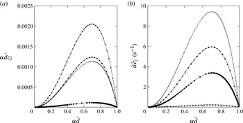
(Rayleigh Reference Rayleigh1892). This can be seen in figure 2, depicting temporal growth rates from linear stability analysis for different parameter configurations (which we will investigate in more detail in this section). Figure 2 shows that our model passes the most basic test, i.e. it accurately predicts the ‘exact’ linear growth rates obtained from the Orr–Sommerfeld problem. In addition to the non-dimensional growth rate in figure 2(a), we have plotted the dimensional one in 2(b) in order to clarify which configuration is the most unstable, as the dimensionless representation is misleading in this respect. Incidentally, it is interesting to note that, although viscous liquids are considered, the most dangerous wavenumber
 ${\it\alpha}_{max}$
corresponds quite closely to the inviscid prediction
 ${\it\alpha}_{max}\bar{d}=2^{-1/2}$
(Rayleigh Reference Rayleigh1892).
Dispersion curves from temporal linear stability analysis. Lines: Orr–Sommerfeld solution; symbols: our model. Gravity-free films in tubes under zero pressure drop for conditions from published work (velocity/length scales:
 $U={\it\sigma}/{\it\mu}_{l}$
;
 $L=R$
). Flow parameters are listed as
 $[\bar{d},\mathit{La}={\it\sigma}{\it\rho}_{l}R/{\it\mu}_{l}^{2},{\it\Pi}_{{\it\rho}},{\it\Pi}_{{\it\mu}}]$
(see also table 2). Here, ●, figure 5(a) Johnson et al. (Reference Johnson, Kamm, Ho, Shapiro and Pedley1991),
 $[0.9,21424,\approx 0,\approx 0]$
;
 $+$
, figure 5(b) Johnson et al. (Reference Johnson, Kamm, Ho, Shapiro and Pedley1991),
 $[0.8,5287,\approx 0,\approx 0]$
; ♦, figure 4(b) Tai et al. (Reference Tai, Bian, Halpern, Zheng, Filoche and Grotberg2011),
 $[0.8,125,\approx 0,\approx 0]$
; ▼, figure 7(b) Tai et al. (Reference Tai, Bian, Halpern, Zheng, Filoche and Grotberg2011),
 $[0.77,0.056,0.95,0.01]$
. (a) Dimensionless growth rate; (b) dimensional growth rate.

Perturbations of the wavenumber
 ${\it\alpha}\bar{d}<1$
may cause an initially smooth liquid film of radius
 $\bar{d}$
to transition towards two distinct deformed equilibrium shapes of constant interfacial curvature (Everett & Haynes Reference Everett and Haynes1972). (i) If the dimensionless liquid volume
 $V_{l}=\tilde{V}_{l}/({\rm\pi}R^{3})=(1-\bar{d}^{2}){\it\Lambda}/R$
is small, the liquid forms a so-called unduloid (Delaunay Reference Delaunay1841). The axial core radius profile
 $d(x)$
of this shape is drawn by the focus of an ellipse with major axis
 $R$
rolled on the tube axis. (ii) If
 $V_{l}>1.73$
, the film forms a liquid bridge, flooding the tube and separating two spherical bubbles (or drops) of the core fluid. The threshold value of
 $V_{l}=1.73$
corresponds to the maximal volume an unduloid can attain and is defined in terms of elliptical integrals in Everett & Haynes (Reference Everett and Haynes1972). Interestingly, and in anticipation of our results, we have found that in thin films that are too thick to form an unduloid (
 $V_{l}>1.73$
), flooding may be significantly delayed (and effectively prevented) due to a buckling mechanism that drastically slows down drainage of the liquid film.
Accurate prediction of flooded states and temporal evolution thitherto is relevant for pulmonary flows in medical science (Grotberg Reference Grotberg1994, Reference Grotberg2011) and water-aided oil recovery from porous rock (Olbricht Reference Olbricht1996). In what follows, we will scrutinize the predictive capabilities of our model in this respect for a variety of fluid combinations. We point out that, in contrast to previous modelling work (Johnson et al. Reference Johnson, Kamm, Ho, Shapiro and Pedley1991; Halpern & Grotberg Reference Halpern and Grotberg2003; Lister et al. Reference Lister, Rallison, King, Cummings and Jensen2006; Halpern et al. Reference Halpern, Fujioka and Grotberg2010), our model takes into account inertia and streamwise viscous diffusion in both phases as well as the full interphase coupling conditions. We will show that these effects are indeed relevant for several realistic fluid pairings.
Figure 3 compares our model predictions for two cases studied by Johnson et al. (Reference Johnson, Kamm, Ho, Shapiro and Pedley1991) (film of mucus liquid in a passive atmosphere) with our own DNS using the VOF (volume of fluid) solver Gerris (Popinet Reference Popinet2009). Therein, the time scale
 ${\it\tau}$
was introduced by Johnson et al. (Reference Johnson, Kamm, Ho, Shapiro and Pedley1991) and is based on an inertialess approximation of the linear temporal growth rate:
 $$\begin{eqnarray}{\it\tau}=6\frac{{\it\mu}_{l}R\bar{d}}{{\it\sigma}}\left[{\it\alpha}^{\ast 4}\left(1/{\it\alpha}^{\ast 2}-1\right)\left(1/\bar{d}-1\right)^{2}\left(1/\bar{d}^{2}-1\right)\right]^{-1},\quad {\it\alpha}^{\ast }={\it\alpha}\bar{d}=\frac{2{\rm\pi}\bar{d}}{{\it\Lambda}/R}.\end{eqnarray}$$
For figures 3(a,b), the liquid volume
 $V_{l}<1.73$
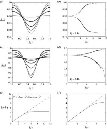
, and indeed both the model and DNS predict the film to evolve towards an unduloid. This is particularly evident in figure 3(b), showing degressive time traces of the minimal and maximal core radii. In figures 3(c,d),
 $V_{l}>1.73$
, and the film evolves towards a liquid bridge, as evidenced by the progressive core-radii time traces. Overall, the agreement in figure 3 between DNS and our model is good. In particular, the evolution of the shape of the film surface (panels a and c) is well predicted. However, the time to flooding (panel d) is slightly underestimated by the model (7 % error). This results from the fact that, with increasing amplitude, the long-wave approximation
 ${\it\Lambda}\gg (1-d)$
is less well fulfilled, explaining why the deviation between model and DNS data gradually increases over time. Meanwhile, figures 3(e,f) show a logarithmic representation of the temporal growth of liquid-collar amplitudes (following Pozrikidis (Reference Pozrikidis1999)) based on the data in figures 3(a,c) respectively. These time traces (solid lines) are compared with a linear growth scenario (dash-dotted lines) based on the temporal growth rate from linear stability analysis (see figure 2). Both lines coincide in the early stages, when the perturbation amplitude is small and growth is governed by linearized mechanics in the vicinity of the base state. At the time point where both curves start to diverge significantly, this linear mechanics no longer holds and a nonlinear description of the film dynamics is necessary. Here, the advantage of the additional complexity of our nonlinear model becomes apparent. Indeed, comparison of figures 3(e,f) with figures 3(b,c) shows that the model yields accurate predictions quite far into the nonlinear growth regime.
Time evolution of annular mucus films in contact with an air core. The parameters correspond to figure 5 in Johnson et al. (Reference Johnson, Kamm, Ho, Shapiro and Pedley1991). (a,b) Formation of a stable unduloid (
 $\bar{d}=0.9$
,
 ${\it\Lambda}/R=6$
,
 $\mathit{La}=2.13\times 10^{4}$
,
 $\hat{d}_{0}=d_{max}|_{t=0}-\bar{d}=0.001$
); (c,d) formation of a liquid bridge (
 $\bar{d}=0.8$
,
 ${\it\Lambda}/R=6$
,
 $\mathit{La}=5.29\times 10^{3}$
,
 $\hat{d}_{0}=0.0025$
). Profiles are displayed at
 $\tilde{t}/{\it\tau}=2,4,5,6,10$
(a) and
 $\tilde{t}/{\it\tau}=1,3,4,5,6,7,7.1$
(c), with
 ${\it\tau}$
according to (3.1) and
 $\mathit{La}=({\it\sigma}R{\it\rho}_{l})/{\it\mu}_{l}^{2}$
. Circles indicate DNS data obtained with the the VOF code Gerris (only available time points are shown in (a) and (c)). Squares highlight the time point displayed in figure 4. (e,f) Logarithmic representation of the linear (dash-dotted line, obtained from stability analysis) and actual (solid line, obtained from the model) growth of interfacial perturbations in (b,d). (a) Film surface evolution; (b) maximal and minimal core radii; (c) film surface evolution; (d) maximal and minimal core radii; (e) linear/nonlinear transition for (b); ( f) linear/nonlinear transition for (d).

Regarding the superposition of model and DNS data in figure 3 and in all subsequent similar figures, a clarification is required. Both simulations were initiated with a sinusoidal perturbation of the core radius
 $d$
at time
 $t=0$
:
 $$\begin{eqnarray}d|_{t=0}=\bar{d}+\hat{d}_{0}\sin (2{\rm\pi}\tilde{x}/{\it\Lambda}).\end{eqnarray}$$
However, the initial perturbation amplitude
 $\hat{d}_{0}$
was chosen differently. To limit the calculation time of our DNS, we imposed a relatively large initial perturbation in these, while our model simulations were initiated with a very small excitation amplitude
 $\hat{d}_{0}$
in order to represent the ‘entire’ time evolution of the flow. In order to compare both time traces, the DNS data were shifted until they matched the model values of the core radii at the first DNS data point. This procedure is only applicable in a time range wherein the interface shape remains close to sinusoidal, which is the case here. We have checked that changing the initial perturbation amplitude
 $\hat{d}_{0}$
of the model calculation to the value of the corresponding DNS produces almost exactly (error
 ${<}1\%$
) the same time traces from there onwards.
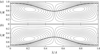
Figure 4 compares the streamlines computed from our model with DNS data for the time point highlighted with a square in figure 3(d). We point out that, in contrast to Johnson et al. (Reference Johnson, Kamm, Ho, Shapiro and Pedley1991), we did not consider a perfectly passive core phase but instead used air in both the model and direct simulations. Indeed, in contrast to previous modelling works, our full account of both fluid phases allows us to obtain the streamlines also in the core phase. Agreement with the DNS data is good, showing that drainage of the liquid film during liquid-bridge formation creates two large counter-rotating vortices, the centre of which is located in the core. The ability to accurately predict these flow structures, which represent an intensification of convective transport, is relevant from the point of view of oxygen transfer in human lung capillaries as well as drying of porous media.
Streamlines in the wall-fixed reference frame obtained from DNS (a) and the WRIBL model (b). Mucus-film/air-core combination. See figure 3(d) and table 2 for the flow conditions and time point (squares in 3(d):
 $\tilde{t}/{\it\tau}=6.1$
). Stream functions are normalized by their maximum and contour line values are identical in both plots, i.e.
 $\pm [0.025,0.1:0.1:0.9]$
.

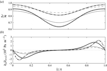
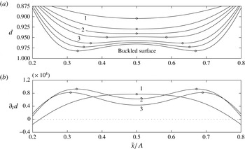
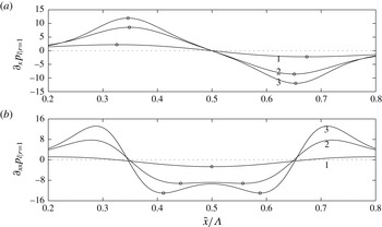
The growth of the collars in figure 3 and the associated vortices in figure 4 are driven by pressure gradients in the liquid that are imposed by variations in free-surface curvature. Figure 5 shows profiles of the axial wall pressure derivative for different time points in figure 3(b,d), i.e. for the unduloid and liquid-bridge scenarios respectively. Circles in this diagram mark DNS data while the dashed (unduloid scenario) and solid (liquid-bridge scenario) lines refer to model predictions. The DNS data are only presented for the latest time point in each case (
 $\tilde{t}/{\it\tau}=5.4,5.6$
) to avoid cluttering the graph. The two earlier time points are included to illustrate the principal difference between the two evolution scenarios. In the liquid-bridge scenario, the pressure derivative increases everywhere as time progresses, constantly increasing the volume of the collar by driving liquid from the film trough. By contrast, the pressure derivative for the unduloid scenario decreases with time in the region of the collar while increasing at the position of the film trough. Comparison of the two time points for this scenario shows that the pressure derivative profile increasingly flattens from within until eventually all pressure variations are nullified and the film reaches the equilibrium shape of an unduloid.
Profiles of the axial wall pressure derivative (b) and the corresponding core-radius distribution (a) for the conditions in figures 3(b) (unduloid scenario:
 $\tilde{t}/{\it\tau}=5.4$
, thick dashed lines) and 3(d) (liquid-bridge scenario:
 $\tilde{t}/{\it\tau}=5.6$
, thick solid lines). Circles mark DNS data and lines model predictions. Thin lines refer to an earlier time point in each case and are not compared with DNS data to avoid cluttering the graph.

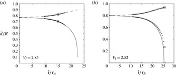
Turning to liquid/liquid film-fluid/core-fluid pairings, figure 6 shows time traces of the extremal core radii for a glycerol/silicone-oil (a) and a water/silicone-oil combination (b). Parameter values are taken from Piroird, Clanet & Quéré (Reference Piroird, Clanet and Quéré2011) and Tai et al. (Reference Tai, Bian, Halpern, Zheng, Filoche and Grotberg2011) respectively. We point out that the time scale in panel (a) is
 ${\it\tau}_{a}={\it\mu}_{l}R/[{\it\sigma}(1-\bar{d})^{3}]$
, chosen to facilitate comparisons with Tai et al. (Reference Tai, Bian, Halpern, Zheng, Filoche and Grotberg2011), while it is defined according to (3.1) in panel (b). In the first case, the film fluid is significantly more viscous than the core fluid, as opposed to the second case where the viscosities are comparable and the viscosity level is lower. In both cases, the liquid volume is sufficiently large to cause flooding and we observe more or less the same evolution as in figure 3(d). Agreement between model and DNS data is again good, the time to flooding being predicted with better accuracy here, due to the fact that
 ${\it\Lambda}/R$
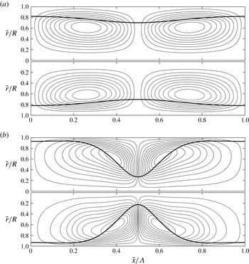
is larger. Figure 7 depicts corresponding streamlines at selected time points and again we remark good agreement between the model and DNS.
Time traces of the minimal and maximal core radii obtained from our model (lines) and DNS (symbols) for two liquid/liquid configurations reported by Piroird et al. (Reference Piroird, Clanet and Quéré2011) and Tai et al. (Reference Tai, Bian, Halpern, Zheng, Filoche and Grotberg2011). (a)
 $\mathit{La}=0.06$
,
 ${\it\Pi}_{{\it\rho}}=0.95$
,
 ${\it\Pi}_{{\it\mu}}=0.01$
,
 $\bar{d}=0.77$
,
 ${\it\Lambda}/R=7.0$
,
 $\hat{d}_{0}=d_{max}|_{t=0}-\bar{d}=0.0023$
; (b)
 $\mathit{La}=66087$
,
 ${\it\Pi}_{{\it\rho}}=1.2$
,
 ${\it\Pi}_{{\it\mu}}=5.6$
,
 $\bar{d}=0.8$
,
 ${\it\Lambda}/R=7.0$
,
 $\hat{d}_{0}=0.0025$
. The Laplace number
 $\mathit{La}={\it\sigma}R{\it\rho}_{l}/{\it\mu}_{l}^{2}$
,
 ${\it\tau}_{a}={\it\mu}_{l}R/[{\it\sigma}(1-\bar{d})^{3}]$
and
 ${\it\tau}_{b}$
according to (3.1). Squares highlight time points considered in figures 7(a,b). (a) Glycerol/silicone oil; (b) water/silicone oil.

Streamlines in the wall-fixed reference frame obtained from DNS (top) and the WRIBL model (bottom). (a) Glycerol/silicone oil:
 $\tilde{t}/{\it\tau}=13.8$
(see the squares in figure 6
a for the time point). (b) Water/silicone oil:
 $\tilde{t}/{\it\tau}=25.6$
(DNS);
 $\tilde{t}/{\it\tau}=25.1$
(WRIBL model) (see the squares in figure 6
b for the DNS time point). Stream functions are normalized by their maximum and contour line values are identical in the DNS and WRIBL plots.

These comparisons give us confidence in the physical soundness of our WRIBL model, which we now employ for a more detailed investigation of the considered gravity-free annular-film/fluid-core arrangement.
3.2. Flooding dynamics: role of inertia and core fluid
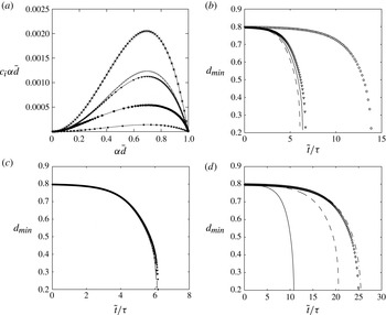
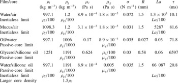
We start by identifying the limits of simplifying assumptions that are frequently made regarding these flows, such as neglecting inertia and considering the core phase as passive. Our results are summarized in figure 8, showing linear growth rates and minimal core-radius time traces for a set of realistic fluid pairings: water/air and mucus/air (b), oil/water and glycerol/silicone oil (c), and water/silicone oil (d). All relevant parameters are quantified in table 3. As a basis for comparison and in contrast to table 2, we have fixed
 $\bar{d}=0.8$
as well as the relative wavelength
 ${\it\Lambda}/(\bar{d}R)$
(by setting
 ${\it\Lambda}$
to the linearly most amplified value). Consequently, the dimensionless liquid volume
 $\tilde{V}_{l}/({\rm\pi}R^{3})$
is constant for all cases. In addition to calculations with realistic parameter values, panels (b–d) also contain results in the inertialess (vanishing fluid densities) and passive-core (
 ${\it\Pi}_{{\it\rho}},{\it\Pi}_{{\it\mu}}\ll 1$
) limits, respectively.
Model predictions of liquid-bridge formation in different limits. (a) Linear dispersion curves obtained from the full model (symbols) and the Orr–Sommerfeld equation (lines) for different fluid pairings given in table 3. Here, ●: water/air; ▼: mucus/air;
 $+$
: oil/water;
 $\star$
: glycerol/silicone oil; ♦: water/silicone oil. (b) Gaseous core (
 ${\it\Pi}_{{\it\rho}},{\it\Pi}_{{\it\mu}}\ll 1$
). Circles (full model) and solid line (inertialess limit): water/air; triangles (full model) and dashed line (inertialess limit): mucus/air. (c) Highly viscous films (
 $\mathit{La},{\it\Pi}_{{\it\mu}}\ll 1$
,
 ${\it\Pi}_{{\it\rho}}\approx 1$
). Stars (full model) and dashed line (passive-core limit): glycerol/silicone oil; pluses (full model) and solid line (passive-core limit): oil/water. (d) Water/silicone oil. Diamonds: full model; solid line: passive core; dashed line: inertialess limit; dot-dashed line: larger core-fluid density.

Parameters from different works used to validate our model. The first two cases correspond to figure 5 in Johnson et al. (Reference Johnson, Kamm, Ho, Shapiro and Pedley1991), who considered a passive core (we use air instead) and specified only dimensionless numbers (we have chosen
 $R$
,
 ${\it\mu}_{l}$
and
 ${\it\rho}_{l}$
as free parameters, assigning plausible values). The last two cases correspond to figures 4(b) and 7(b) in Tai et al. (Reference Tai, Bian, Halpern, Zheng, Filoche and Grotberg2011). Where necessary,
 ${\it\Lambda}/R$
was rounded to the nearest integer to facilitate DNS with Gerris.

Parameters for the liquid-bridge formation scenarios in figure 8:
 $\bar{d}=0.8$
,
 $\mathit{La}={\it\sigma}{\it\rho}_{l}R/{\it\mu}_{l}^{2}$
,
 ${\it\tau}$
according to (3.1). The wavelength in all cases corresponds to the linearly most amplified value in figure 8(a). The values of the Reynolds number
 $\mathit{Re}_{F}={\it\rho}_{l}R^{2}/({\it\mu}_{l}{\it\tau}_{F})$
based on the time to flooding
 ${\it\tau}_{F}$
are 17.8, 1.4 and 4.8 for the water/air, mucus/air and water/silicone-oil scenarios respectively, while
 $\mathit{Re}_{F}\ll 1$
for the highly viscous films.

For the two liquid/gas pairings (b), the core fluid is practically passive in reality so that the passive-core limit need not be investigated further. On the other hand, the Laplace number, which relates inertia and driving capillary to stabilizing viscous forces, is very large here and, consequently, inertia is expected to be relevant. This is confirmed by the core-radius time traces in figure 8(b), showing inertialess predictions to underestimate the time to flooding. For the water/air combination (
 $\mathit{La}\approx 10^{5}$
) the error is significant (
 ${\approx}60~\%$
), while it is smaller (
 ${\approx}10~\%$
) for the mucus/air pairing (
 $\mathit{La}\approx 10^{3}$
). In the inertialess limit, the liquid film reacts immediately to the resulting driving force (difference between capillary-induced pressure gradients and viscous stresses), which is quantified by
 $\mathit{La}$
, and, thus, as
 $\mathit{La}$
increases, the inertialess prediction of the time to flooding is increasingly too short. The relevance of inertia can also be inferred from the Reynolds number
 $\mathit{Re}_{F}={\it\rho}_{l}R^{2}/({\it\mu}_{l}{\it\tau}_{F})$
based on the time to flooding
 ${\it\tau}_{F}$
, which was obtained from figure 8. Indeed, for the water/air, mucus/air and water/silicone-oil scenarios
 $\mathit{Re}_{F}=17.8$
, 1.4 and 4.8 respectively, while
 $\mathit{Re}_{F}\ll 1$
for the highly viscous films.
When the liquid film is very viscous and much more so than the core fluid, as is considered in figure 8(c),
 $\mathit{La}$
is low and inertia is insignificant. In addition, viscous dissipation in the core fluid is negligible compared with the film so that the core phase is effectively passive. This limit is shown to give very precise predictions of the film evolution for the oil/water and glycerol/silicone-oil combinations. Interestingly, all four curves in this plot collapse, due to the choice of the time scale
 ${\it\tau}$
(3.1), which is pertinent in the inertialess passive-core limit (Johnson et al.
Reference Johnson, Kamm, Ho, Shapiro and Pedley1991).
Figure 8(d) concerns a more complicated fluid combination, i.e. a water film and a silicone-oil core. In this case,
 $\mathit{La}$
is large and the densities and viscosities of the two fluids are comparable. Consequently, neither the inertialess (20 % error) nor the passive-core (60 % error) limit predicts the film evolution accurately. As inertia clearly is relevant in this case, we have also checked the influence of the density ratio by increasing the core density by 50 % with respect to the liquid. The resulting time trace in figure 8(d) (dot-dashed line) predicts a longer time to flooding than for the lower density ratio. This excludes any relevance of the Rayleigh–Taylor instability, which would instead increase the growth rate with increasing
 ${\it\Pi}_{{\it\rho}}$
. We thus conclude that the increased physical complexity of our model, i.e. accounting for inertia, an active fluid core and full coupling between the two phases, is indeed useful/necessary to capture the flooding dynamics of real configurations such as core–annular arrangements of water/air and water/silicone oil.
3.3. Delay of flooding by the viscous-blocking mechanism
We turn now to a compelling phenomenon that we have encountered when simulating flooding scenarios for thin liquid films that are too thick to form unduloids. In these cases,
 $V_{l}>1.73$
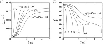
and flooding should (eventually) occur according to the criterion discussed at the beginning of this section (Everett & Haynes Reference Everett and Haynes1972). Figure 9 shows time traces of the perturbation amplitude
 $d_{max}-\bar{d}$
and the minimal core radius
 $d_{min}$
for such a case. More precisely, the parameter values correspond to one of the situations studied by Halpern & Grotberg (Reference Halpern and Grotberg2003), i.e.
 $R=0.3~\text{mm}$
,
 $\mathit{La}=0.01$
,
 ${\it\Pi}_{{\it\rho}}=0.001$
,
 ${\it\Pi}_{{\it\mu}}=0.002$
and
 ${\it\Lambda}/R=7.73$
. The different data sets in figure 9 correspond to different values of
 $\bar{d}$
, which was varied to control the liquid volume (specified next to the respective graphs). At large liquid volumes (
 $V_{l}\geqslant 2.28$
), the usual flooding scenario occurs. This is characterized by a progressive decline of
 $d_{min}$
until the formation of a liquid bridge. When
 $V_{l}$
is reduced (
 $V_{l}\leqslant 2.14$
), the time traces of
 $d_{min}$
develop a point of inflexion, marking a change from a progressive to a degressive growth of the liquid collar. For sufficiently large liquid volumes (
 $V_{l}>2.01$
), this does not prevent the formation of a liquid bridge, as a second point of inflexion develops later and leads the evolution back to a progressive growth scenario. However, for
 $V_{l}<2.01$
and particularly
 $V_{l}=1.88$
, the growth at large times is entirely degressive and flooding seems to be infinitely delayed and thus effectively avoided. This is a surprising result because
 $V_{l}>1.73$
and thus there are always curvature variations (and associated pressure variations) along the film surface (Everett & Haynes Reference Everett and Haynes1972) that drive the liquid within the film from troughs to humps (as the situation is unstable to the Plateau–Rayleigh mechanism).
Transition between fast and slow flooding dynamics as the liquid volume, controlled through
 $\bar{d}=[0.80,0.84,0.85,0.855,0.86,0.87]$
, decreases. All other properties are maintained constant. The film/core-fluid pairing is mucus/air (Halpern & Grotberg Reference Halpern and Grotberg2003):
 $\mathit{La}={\it\sigma}{\it\rho}_{l}R/{\it\mu}_{l}^{2}=5287$
,
 ${\it\Pi}_{{\it\rho}}=0.001$
,
 ${\it\Pi}_{{\it\mu}}=0.002$
,
 ${\it\Lambda}/R=7.73$
,
 $\hat{d}_{0}=d_{max}|_{t=0}-\bar{d}=0.0013$
. The maximal liquid volume of an unduloid is
 $\tilde{V}_{l}/({\rm\pi}R^{3})=1.73$
(Everett & Haynes Reference Everett and Haynes1972). The square relates to figure 10. (a) Maximal core radius; (b) minimal core radius.

A closer look at the evolution of the film surface is thus required and we do this for the case
 $V_{l}=1.88$
. Due to the relevance of this case for our paper, we have also included a comparison with DNS data in appendix D (see figure 18). Figure 10 shows axial profiles of the film surface
 $d(x)$
in the vicinity of the liquid-film trough, i.e. the point of maximal core radius and minimal film thickness, at different time points (remark: the radial coordinate is decreasing in this graph). On inspecting the different profiles from top to bottom, i.e. in the order of increasing time, a change in shape is observable. The two topmost profiles have an axially concave shape throughout, the third exhibits a flat portion in the middle and from the fourth profile onwards the film surface has buckled, creating a small lobe in the middle flanked by two new troughs that grow thinner with increasing time. The transition time point between the unbuckled/buckled shape is
 $\tilde{t}=1.82~\text{s}$
and corresponds to the third profile from the top. This point is highlighted with a square in figure 9(b) and coincides with the inflexion point of the core-radius time trace. Buckling thus causes the change in flooding dynamics and we proceed to explain its mechanism.
Buckling of the film trough. (a) Time evolution of the film surface (remark: radial coordinate is decreasing) for
 $\tilde{t}=[1.32~(1),1.65,1.82~(2),1.98~(3),2.31,2.64,3.30~(\text{bottom})]~\text{s}$
. The uppermost four profiles show a transition from an axially concave towards a convex shape, passing through a straight interface. This profile (2) signifies the onset of buckling and the corresponding time point (
 $\tilde{t}=1.82~\text{s}$
) is highlighted in figure 9 with a square. (b) Profiles of the core-radius time derivative (
 $t=\tilde{t}{\it\mu}_{l}{\it\rho}_{l}^{-1}R^{-2}$
) at
 $\tilde{t}=1.32~\text{s}$
(1),
 $\tilde{t}=1.82~\text{s}$
(2) and
 $\tilde{t}=1.98~\text{s}$
(3). Circles highlight loci of minimal core radius and maximal growth rate.

A purely kinematic view is provided in figure 10(b), depicting profiles of the core-radius growth rate
 $\partial _{t}d$
at selected time points in figure 10(a). In the early stages when the liquid film is still relatively thick (
 $\tilde{t}=1.32~\text{s}$
, profile 1), the growth rate is maximal at the trough and decreases monotonically moving outward, which tends to preserve the concave shape of the film surface. With increasing time, however, the flow in the film trough, the first locus to ‘feel’ the presence of the approaching wall, is increasingly affected by viscous forces, generating a dip in growth rate there (profiles 2 and 3). In this region, the axial flow closely approaches lubrication conditions and the liquid flow rate
 $q_{l}$
can be expressed in terms of the liquid wall pressure gradient (for convenience, we assume
 ${\it\Pi}_{{\it\rho}}={\it\Pi}_{{\it\mu}}=0$
here):
 $$\begin{eqnarray}q_{l}=\partial _{x}p_{l}|_{r=1}\frac{{\rm\pi}\mathit{Re}_{l}}{8}\left[-1+4d^{2}+d^{4}(-3+4\log d)\right],\end{eqnarray}$$
which, with the help of (2.2), yields the growth rate
 $\partial _{t}d$
:
 $$\begin{eqnarray}\left.\begin{array}{@{}c@{}}\partial _{t}d=\mathit{Re}_{l}\left[A(d)\partial _{x}p_{l}|_{r=1}\partial _{x}d+B(d)\partial _{xx}p_{l}|_{r=1}\right],\\ \displaystyle A(d)=\frac{1}{2}\left[1+d^{2}(-1+2\log d)\right],\quad B(d)=\frac{1}{16d}\left[-1+4d^{2}-d^{4}(3-4\log d)\right].\end{array}\!\right\}\end{eqnarray}$$
The monotonic functions
 $A(d)\geqslant 0$
and
 $B(d)\leqslant 0$
both approach zero as
 $d\rightarrow 1$
. However,
 $B(d)$
does so more rapidly than
 $A(d)$
and thus the growth rate
 $\partial _{t}d$
is dominated by
 $\partial _{x}p_{l}|_{r=1}$
for very thin films, unless the gradient
 $\partial _{x}d$
is small. Importantly, however,
 $\partial _{x}d=\partial _{x}p_{l}|_{r=1}=0$
at the film trough due to symmetry and so the second pressure derivative always controls growth there. Figure 11(b) shows that
 $\partial _{xx}p|_{r=1}$
is large and negative at the film trough, explaining the initially large
 $\partial _{t}d$
there. However, as
 $|B(d)|$
monotonically decreases with increasing
 $d$
(due to increasing viscous flow resistance),
 $\partial _{t}d$
at the trough must decrease with time, explaining the dip in profiles 2 and 3 of figure 10(b).
Profiles of the first (a) and second (b) axial wall pressure derivatives for the three numbered profiles in figure 10. The growth rate
 $\partial _{t}d$
in (3.4) is dominated by
 $\partial _{x}p_{l}|_{r=1}$
where
 $\partial _{x}d$
is large, while
 $\partial _{xx}p_{l}|_{r=1}$
is dominant where
 $\partial _{x}d$
is small. Circles highlight relevant extremal values.

Viscous slowing of growth in the region of the film trough causes the flattening of the film surface discernible between profiles 1 and 2 in figure 10(a). This in turn has two consequences that are relevant for the subsequent growth dynamics. (i) At the extremities of the flat portion of profile 2 (
 $\tilde{x}/{\it\Lambda}\approx 0.4,0.6$
) either side of the film trough, the second pressure derivative in figure 11(b) develops minima. Because growth in the flat film region is dominated by the second pressure derivative,
 $\partial _{t}d$
there increases relative to the trough. As a consequence, the film surface buckles, forming two new troughs at these positions (profile 3 and onwards in figure 10
a). (ii) As the flat portion of the film surface profile extends outward, the steepness
 $\partial _{x}d$
of the outlying portions (
 $\tilde{x}/{\it\Lambda}<0.4,\tilde{x}/{\it\Lambda}>0.6$
) strongly increases, which, according to (3.4), amplifies growth there due to the first pressure derivative. This effect causes
 $\partial _{t}d$
in figure 10(b) to attain global maxima at
 $\tilde{x}/{\it\Lambda}\approx 0.3,0.7$
, where the axial pressure gradient, plotted in figure 11(b), is large and positive. This large growth rate causes the flat and later the buckled portion of the film surface to keep extending outward, explaining the gradual displacement of the buckling-induced film troughs as time progresses (profile 3 and onwards in figure 10
a).
From the point of view of the flooding dynamics in figure 9(b), the most relevant feature of the buckling mechanism is that it eventually produces two very thin film troughs at
 $\tilde{x}/{\it\Lambda}\approx 0.3,0.7$
, which act as bottlenecks in the subsequent growth scenario. Indeed, liquid required to sustain the growth of the large collars needs to pass through these bottlenecks, which will grow even thinner as time goes on. This explains both the extreme slowness of growth in figure 9(b) for
 $\tilde{t}>1.82~\text{s}$
(we are still considering the case
 $V_{l}=1.88$
) and its degressive nature.
In summary, unstable thin liquid films can thus drastically delay the formation of a liquid bridge even if their volume is too large to form an unduloid. In contrast to small-volume liquid films, which evolve into static unduloids, arrest of growth is not achieved through a decrease in the driving force (i.e. capillary pressure gradients) but rather through viscous dissipation. More precisely, the liquid film forms an interfacial shape that maximizes this dissipation by generating a buckled surface between two very thin troughs, acting as bottlenecks. This buckled surface, due to its local extrema, is not compatible with the definition of an unduloid. We thus believe that the delay of flooding observed in figure 9(b) is caused by a distinct mechanism, rather than being the result of approaching the threshold for the existence of unduloids as the liquid volume decreases.
It is interesting to compare these observations with the drainage of small-volume liquid films investigated by Lister et al. (Reference Lister, Rallison, King, Cummings and Jensen2006). Indeed, there also, thin lobes separating large collars were found to impose very slow evolution dynamics. However, in contrast to our work, Lister et al. (Reference Lister, Rallison, King, Cummings and Jensen2006) considered films in the limit
 $V_{l}\rightarrow 0$
, i.e. films that may form unduloids. Our observations are complementary in that they show that liquid films of sufficiently large volume that they cannot reach an equilibrium shape other than a liquid bridge can be effectively prevented from flooding by a viscous-blocking mechanism. We also point out that the buckled shapes represented in figure 10(a) closely resemble the saturated interfacial shapes observed by Yiantsios & Higgins (Reference Yiantsios and Higgins1989) for liquid films subject to the Rayleigh–Taylor instability.
Total (dimensionless) viscous force per unit area
 $F_{x{\it\mu}}^{\prime \prime }$
acting on the axial cross-section of the liquid film (3.5) related to the (dimensionless) pressure jump
 $\mathit{We}^{-1}$
across a free surface of core radius
 $d=1$
(the length scale being
 $L=R$
). Negative values (circles mark changes of sign) indicate deceleration of the liquid (
 $\partial _{x}u<0$
) as it moves away from the film trough in the centre (see figure 10(a) for film surface profiles). This produces an axial viscous force compressing the liquid between the considered position and its mirror on the other side of the trough.

For completeness, we discuss the role of two other effects that immediately come to mind with regard to the buckling mechanism. First, the secondary lobe emerging from the buckled surface in figure 10(a) could conceivably result from a primary Plateau–Rayleigh instability of the flat film forming at the trough. However, as the length of the lobe is approximately
 $l=0.4{\it\Lambda}=3.1R$
, i.e. smaller than the circumference of the film surface there,
 $2{\rm\pi}0.925R=5.8R$
, this hypothesis must be discarded. Formation of the secondary lobe, although similar in appearance, is thus mechanically different from the formation of a satellite drop in the core fluid as may occur during liquid-bridge formation. In the latter case, the core radius is very small and thus the Plateau–Rayleigh mechanism is dominant. Second, the term ‘buckling’ in a fluid-mechanical context is generally used when viscous normal stresses cause a fluid flow confined by a free surface to deviate from its (unstable) primary configuration (Suleiman & Munson Reference Suleiman and Munson1981; Yarin & Tchadarov Reference Yarin and Tchadarov1996; Ribe Reference Ribe2002; Slim et al.
Reference Slim, Balmforth, Craster and Miller2009; Ribe Reference Ribe2012; Slim, Teichman & Mahadevan Reference Slim, Teichman and Mahadevan2012). In analogy to buckling of solid plates or rods, this only occurs when the viscous stresses are compressive, i.e.
 $2{\it\mu}\partial _{x}u<0$
, which means that the flow must be decelerating. To check whether the thin film in the region of the trough represented in figure 10 is indeed axially compressed by normal viscous stresses, figure 12 depicts profiles of the total (dimensionless) axial viscous force per unit area,
 $F_{x{\it\mu}}^{\prime \prime }$
, acting on the cross-section of the film (more precisely, the cross-section in which the normal is oriented away from the film trough):
 $$\begin{eqnarray}F_{x{\it\mu}}^{\prime \prime }=\tilde{F}_{x{\it\mu}}^{\prime \prime }/({\it\rho}_{l}U^{2}),\quad \tilde{F}_{x{\it\mu}}^{\prime \prime }=-\frac{1}{{\rm\pi}(R^{2}-\tilde{d}^{2})}\int _{\tilde{d}}^{R}2{\rm\pi}\tilde{r}(2{\it\mu}_{l}\partial _{\tilde{x}}\tilde{u} )\text{d}\tilde{r}.\end{eqnarray}$$
In figure 12,
 $F_{x{\it\mu}}^{\prime \prime }$
is related to a representative (dimensionless) liquid pressure
 $P$
, which we have chosen as the pressure jump across a cylindrical film surface of dimensional radius
 $R$
. By choosing the length and velocity scales for non-dimensionalization as
 $L=R$
and
 $U={\it\mu}_{l}/({\it\rho}_{l}R)$
, we obtain
 $P=\mathit{We}^{-1}$
. Figure 12 instructs us that, although viscous compressive forces act in the outer regions either side of the film trough, their magnitude is relatively small compared with pressure forces and, thus, viscous buckling is not of significant importance here.
Next, we attempt to provide a quantitative criterion for the onset of the viscous-blocking mechanism. If it is assumed that the wavelength of the free-surface perturbation corresponds to the linearly most amplified value, i.e.
 ${\it\Lambda}/R\approx 2{\rm\pi}\bar{d}2^{1/2}$
, and that the core phase is more or less passive, i.e.
 ${\it\Pi}_{{\it\rho}},{\it\Pi}_{{\it\mu}}\ll 1$
, there are only two remaining influencing parameters: the mean core radius
 $\bar{d}$
and the Laplace number
 $\mathit{La}={\it\sigma}{\it\rho}_{l}R/{\it\mu}_{l}^{2}$
. While the effect of
 $\bar{d}$
has been previously established in figure 9, figure 13 illustrates the effect of
 $\mathit{La}$
. Intriguingly, the viscous-blocking mechanism seems to be insensitive to
 $\mathit{La}$
, which after all was varied over two orders of magnitude. Although the dimensional temporal growth quickens with increasing Laplace number, the dimensionless core-radius time traces in panel (a) collapse perfectly if the time scale
 ${\it\tau}$
according to (3.1) is used for non-dimensionalization. Consequently, all time traces illustrate the same physics, i.e. a point of inflexion and a degressive growth behaviour at large times, indicating viscous blocking. Moreover, panel (b) shows that the same buckled interfacial shape is attained for all
 $\mathit{La}$
values at sufficiently large times. We thus conclude that the limit
 $\bar{d}\gtrapprox 0.86$
established in figure 9(b) is a sufficient criterion for the onset of viscous blocking.
Insensitivity of the viscous-blocking mechanism to the Laplace number
 $\mathit{La}={\it\sigma}{\it\rho}_{l}R/{\it\mu}_{l}^{2}$
, which was varied across two orders of magnitude:
 $\mathit{La}=91.8=\mathit{La}_{0}$
(solid line);
 $\mathit{La}=10\cdot \mathit{La}_{0}$
(circles) and
 $\mathit{La}=100\cdot \mathit{La}_{0}$
(pluses). (a) Minimal core radius as a function of time scaled with
 ${\it\tau}$
according to (3.1); (b) buckled profiles at
 $\tilde{t}/{\it\tau}=9.9$
.

Although the viscous-blocking mechanism discussed above drastically slows down the growth of large liquid collars, the thermodynamic criterion of Everett & Haynes (Reference Everett and Haynes1972) predicts that eventually, i.e. for sufficiently long times, the liquid film in figure 9(b) (
 $V_{l}=1.88$
) must form a liquid bridge. To investigate the dynamics leading to this event, we have performed several long-time model simulations. Figure 14 depicts time traces of the minimal core radius obtained from these long-time simulations. We start by concentrating on the solid line, which shows that, for times exceeding the interval displayed in figure 9(b),
 $d_{min}$
continues to grow degressively for a very long time, until it reaches a plateau value at
 $\tilde{t}=90~\text{s}$
. During this time, the film thickness profile remains almost unchanged. Subsequently, starting at
 $\tilde{t}=90~\text{s}$
, the dynamics in the region of the film trough starts to play a decisive role. This is illustrated by numbered insets in figure 14, displaying the time evolution of the film surface in this region at representative time points in the core-radius time trace (highlighted by filled circles and numbers corresponding to the respective insets). This shows that, from the third profile onwards, the symmetry of the film surface is broken, producing a shallower trough on the right than on the left. At the same time, the film surface starts to slide to the right. This motion further increases the asymmetry, whereby the right trough evolves into a very thin and increasingly elongated residual film, while the left trough noticeably thickens. Thereby, the elongated residual film drains into the neighbouring large liquid collar as a result of its small axial interfacial curvature. This causes the latter to grow and eventually form a liquid bridge.
Long-time evolution of the minimal core radius for the case in figure 9(b):
 $\tilde{V}_{l}/({\rm\pi}R^{3})=1.88$
. Flooding occurs only at very long times due to symmetry breaking in the region of the film trough, which subsequently produces a sliding motion of the liquid film (
 $\tilde{t}>70~\text{s}$
). This kickstarts the growth of large liquid collars anew and eventually leads to the occlusion of the tube. These events are illustrated by insets, showing the time evolution of the film trough in a magnified view (the horizontal line corresponds to the tube wall and the displayed axial and radial intervals are
 $\tilde{x}/{\it\Lambda}\in [0,1]$
and
 $\tilde{r}/R\in [0.95,1]$
respectively). The dot-dashed line relates to the limit
 $J_{i}=K_{i}=L_{i}=M_{i}=0$
in (2.33), when axial normal viscous stresses are not accounted for. Different types of perturbations cause the symmetry breaking for the dashed (numerical errors) and solid/dot-dashed (minute gravitational acceleration
 $g_{res}=10^{-10}~\text{m}~\text{s}^{-2}$
) lines, respectively.

Effect of the symmetry-breaking and sliding episodes in figure 14 on the flow pattern in the liquid film and core flow. Liquid-film conditions correspond to figure 14, while for the core flow (3.6)
 $L_{T}=0$
. (a) Symmetrical flow:
 $\tilde{t}=1.98~\text{s}$
; (b) breaking of symmetry:
 $\tilde{t}=66.09~\text{s}$
; (c) pinch-off:
 $\tilde{t}=84.27~\text{s}$
; (d) cellular pattern:
 $\tilde{t}=99.14~\text{s}$
.

In order for symmetry to break in a macroscopically symmetrical system like our static film/core arrangement, two conditions must be fulfilled: (i) the film shape shown in inset 2 of figure 14 must be unstable to small non-symmetrical perturbations and (ii) such perturbations must exist in the first place. In any numerical simulation, the accumulation of numerical errors over long simulation times eventually produces sufficiently large perturbations to disturb an unstable flow. In our case, this is demonstrated by the dashed line in figure 14, where symmetry breaking occurs solely due to numerical errors. However, the nature and amplitude of numerical errors are difficult to control in a numerical simulation as they depend on many factors, ranging from minute changes in resolution to the type of machine the simulation is run on. In our specific case, this can change the sliding direction of the liquid film once the symmetry has been broken. To exert more control on the source of perturbations eventually causing the symmetry breaking, the simulation underlying the solid line in figure 14 (as well as the dot-dashed line) was performed with a minute residual gravitational acceleration
 $g=g_{res}=10^{-10}~\text{m}~\text{s}^{-2}$
by accordingly setting the Froude number
 $\mathit{Fr}=U/(gR)^{1/2}$
in (2.33) (this also applies to the simulations in figures 15–17). Compared with the purely gravity-free simulation (dashed line), the temporal evolution is identical in the early stages and differs only in terms of the eventual onset of symmetry breaking as well as the direction of the resulting sliding motion of the liquid film. Indeed, in the simulation with residual gravity (solid line), the film always slides in the direction of
 $g_{res}$
(which we have checked by testing
 $g=-g_{res}$
) and the onset of symmetry breaking occurs somewhat earlier than in the purely gravity-free case, where it is exclusively caused by numerical errors. Interestingly, residual gravity may actually be present in space experiments (Hamacher, Fitton & Kingdon Reference Hamacher, Fitton and Kingdon1987) due to ‘
 $g$
-jitter’ (typically acceleration variations of
 $10^{-4}g_{earth}$
), and we see here that it may be strong enough to break the symmetry of a static film/core arrangement. Our simulations with and without residual gravity also lead us to conclude that symmetry breaking results from an unstable film surface configuration, when the newly formed troughs in figure 14 (see insets) become very thin. In our numerical code, a centred second-order finite difference scheme was used for spatial discretization and an adaptive time step Crank–Nicholson scheme for time discretization. As opposed to Lister et al. (Reference Lister, Rallison, King, Cummings and Jensen2006), no local spatial refinement of very thin film regions was performed, our axial grid being equidistant. As a consequence, our simulations required a large number of grid points to resolve the thin-film dynamics. The wavelength of the film in figure 14 was axially resolved with
 $N_{x}=500$
points and the grid dependence was checked, for the solid line, by comparing with an
 $N_{x}=2000$
simulation. The onset of sliding is only slightly affected (i.e. slightly delayed) by this fourfold refinement.
Effect of an oscillating core flow (3.6) on liquid-film dynamics. Time traces of the minimal core radius (a) and the axial position of the centre of liquid mass (b) according to (3.7). Dashed line: no core-flow oscillation (
 $\tilde{L}_{T}=0$
); solid line: core-flow oscillation with
 $\tilde{f}=1/3~\text{Hz}$
,
 $\tilde{L}_{T}=7.73~R$
; dot-dashed lines: corresponding first-order model predictions (
 $J_{i}=K_{i}=L_{i}=M_{i}=0$
in (2.33)).

Flow patterns for the case of an oscillating core flow (3.6) in figure 16 at time points
 $\tilde{t}=2.97$
, 4.49, 20.00 and 34.04 s (as displayed in panels (b) to (e)). The insets show a magnified view of the film trough region. Panel (a) shows the time evolution of the total (solid line) and core (filled circles) flow rate, highlighting the time points of the streamline plots with squares. Flow rates are non-dimensionalized with
 ${\it\mu}_{l}R/{\it\rho}_{l}$
.

Interestingly, axial normal viscous stresses play an important role in the dynamics of the film trough evolution. This is illustrated by the dot-dashed line in figure 14, which represents data obtained with our model in the limit
 $J_{i}=K_{i}=L_{i}=M_{i}=0$
of (2.33), i.e. when axial normal viscous stresses are not accounted for. Indeed, this first-order model predicts flooding at a much earlier time than the full formulation, an observation in line with studies of falling liquid films where first-order integral boundary layer models have been shown to overpredict the amplitude of capillary waves preceding large wave humps (Ruyer-Quil & Manneville Reference Ruyer-Quil and Manneville2000). In our case, we have checked that the inclusion of viscous stresses mainly affects the onset of the symmetry breaking in the film trough region. We thus conclude that the (simplified) second-order WRIBL model we have introduced in this paper is necessary to accurately predict the nonlinear dynamics of gravity-free liquid-film/core-fluid arrangements in narrow tubes.
Finally, it is to be expected that the symmetry-breaking dynamics in the film trough will generate intricate flow structures in the core phase. These can be captured by our model, which fully accounts for both phases. We proceed to a detailed investigation of the core-flow dynamics as well as its interaction with the liquid film in the following section.
3.4. Low-frequency core-flow oscillations
To conclude this section, we consider the dynamics of the core flow and its interaction with the liquid film. For this, we prescribe a harmonic temporal oscillation of the total flow rate in our model simulations:
 $$\begin{eqnarray}q_{tot}=q_{l}+q_{g}=2{\rm\pi}fL_{T}\left({\rm\pi}R^{3}\right)\sin \left(2{\rm\pi}ft\right).\end{eqnarray}$$
For the case of gravity-free liquid films in interaction with a gaseous core this condition amounts to imposing the core flow rate
 $q_{g}$
, because
 ${\it\Pi}_{{\it\mu}}\ll 1$
and thus
 $q_{g}\gg q_{l}$
. The control parameters in (3.6) are
 $L_{T}=\tilde{L}_{T}/R$
, denoting the dimensionless stroke length (i.e. the stroke required to generate the oscillating flow with a piston pump), as well as the dimensionless oscillation frequency
 $f$
. We recall that Halpern & Grotberg (Reference Halpern and Grotberg2003) considered a similar situation in their investigation of pulmonary liquid films. However, the model they employed was limited to high oscillation frequencies
 $f$
, which the authors found to produce a stabilizing effect regarding the formation of liquid bridges. We, on the other hand, consider low oscillation frequencies, of the order imposed by the breathing rate in human lungs (
 $\tilde{f}\approx 1/3~\text{Hz}$
). In this range, we find the core-flow oscillation to have a destabilizing effect, and thus our work is complementary to Halpern & Grotberg (Reference Halpern and Grotberg2003).
We start by setting
 $L_{T}=0$
, whereby we recover the flow scenario represented in figure 14, and investigate the flow patterns produced in the core flow during the symmetry-breaking and sliding episodes discussed in the previous subsection. Accordingly, figure 15 represents streamlines for four representative time points in figure 14, i.e.
 $\tilde{t}=1.98$
, 66.09, 84.27 and 99.14 s. In figure 15(a), showing the earliest time, the flow pattern remains symmetrical. It is characterized by two counter-rotating vortices driven by the growth of the liquid collar, which is fed by the film troughs on either side. As these film troughs grow thinner (b), the two vortices develop a radially elongated core. At the same time, symmetry in the flow pattern is lost, while one of the two vortices expands sideways, compressing its neighbour in the process. Interestingly, the film surface still appears to be symmetrical at this stage, at least to the eye (see also figure 14). Then, as the left film trough in figure 15(c) (the right film trough in profile 4 of figure 14) becomes significantly more pronounced than its counterpart, the left vortex starts to pinch off. This eventually produces a cellular pattern of four vortices, as shown in figure 15(d). As time progresses (not shown here), the left film trough increasingly flattens (see the right trough in profile 6 of figure 14), producing an increasing number of counter-rotating vortices at that position.
Turning to a more complicated scenario, figure 16 compares the case of an oscillating core flow,
 $\tilde{f}=1/3~\text{Hz}$
and
 $\tilde{L}_{T}=7.73R$
, with the quiescent core case in figure 14. Figure 16(a) represents time traces of the minimal core radius, showing that the onset of flooding occurs drastically sooner in the presence of an oscillatory core flow. We also note that the dot-dashed lines, which were obtained from the first-order model (
 $J_{i}=K_{i}=L_{i}=M_{i}=0$
in (2.33)), confirm the importance of accounting for streamwise normal viscous stresses, as both lines significantly deviate from the respective full-model results. The earlier onset of flooding in the case with core-flow oscillations results from an earlier onset of the axial sliding observed in figure 14. This is shown in figure 16(b), displaying time traces of the axial position
 $x_{c}$
of the liquid centre of mass for the two cases in figure 16(a):
 $$\begin{eqnarray}x_{c}=\frac{\displaystyle \int _{d}^{{\it\Lambda}/R}{\rm\pi}(1-d^{2})x\text{d}x}{\displaystyle \int _{d}^{{\it\Lambda}/R}{\rm\pi}(1-d^{2})\text{d}x}.\end{eqnarray}$$
This plot confirms that sliding occurs earlier for the case with core-flow oscillation. Moreover, the signature of this oscillation is discernible in the corresponding time trace of
 $x_{c}$
. This shows that the core flow causes the film to briefly move back and forth in the very early stages before the sliding motion sets in, whereafter the core flow merely causes a periodic slowing and acceleration of this motion. The earlier onset of sliding results from an earlier breakdown of symmetry due to the back and forth motion imposed by the core flow. This oscillatory state is more unstable with respect to the minute residual gravity present in our simulations (which once again determines the direction of the sliding motion) due to the effect of axial inertia. Meanwhile, the dot-dashed lines in figure 16(b) once again confirm the importance of axial normal viscous stresses.
Finally, we use our full two-phase model to investigate the time evolution of the flow pattern in the presence of core-flow oscillations. Figure 17 represents streamlines at four representative time points for the case with core-flow oscillation in figure 16, i.e.
 $\tilde{f}=1/3~\text{Hz}$
and
 $\tilde{L}_{T}=7.73R$
in (3.6). These time points are highlighted with squares in figure 17(a), displaying time traces of the total (solid line) and core (filled circles) flow rates. Incidentally, this plot confirms the above-introduced conjecture that the total flow rate oscillation (3.6) amounts to imposing an oscillation of the core flow rate, as indeed the two time traces are indistinguishably close.
Figures 17(b,c) correspond to the early stages of the liquid-film evolution (see also figure 16 a). In this stage, the growth rate of the liquid collar is large and the liquid flow is dominated by the growth dynamics, i.e. the draining of the film trough towards the liquid collar. This produces a cellular flow similar to that in figure 15(a), at least within the liquid. However, the flow pattern in the core is quite different and is strongly affected by the temporal oscillation. Indeed, small vortices intermittently form on either side of the liquid collar depending on the direction of the core flow. More precisely, the vortices occur on the downstream side of the collar. Once the growth of the liquid collar has slowed, the core flow influences the liquid flow pattern to a larger extent, as shown in figures 17(d,e). In figure 17(d), the core flow is directed from right to left. The liquid film, however, is moving to the right as the sliding motion discussed with respect to figure 16(b) has already begun. These opposing flow directions produce a vortex in the crest of the liquid collar, circulating liquid within the film in the counter-clockwise direction. At this stage, the film trough on the left of the collar has already become very thin, generating a small counter-clockwise vortex at this position (see the inset, showing a magnified view). In figure 17(e), the core flow is oriented from left to right and thus supports the liquid sliding motion. Interestingly, liquid in the elongated film trough (which has significantly elongated at this stage) flows from right to left, creating a separation zone, which is further subdivided into several clockwise vortices.
4. Conclusion
We have considered the axisymmetric arrangement of a liquid film, lining the inner surface of a narrow cylindrical tube, in interaction with an active core-fluid flow. For this configuration, we have derived a (simplified) second-order low-dimensional model by applying the long-wave WRIBL approach (Ruyer-Quil & Manneville Reference Ruyer-Quil and Manneville2002; Kalliadasis et al. Reference Kalliadasis, Ruyer-Quil, Scheid and Velarde2012) to both fluid phases, while fully accounting for interphase coupling. In this, the current work is an extension of the work by Dietze & Ruyer-Quil (Reference Dietze and Ruyer-Quil2013), who considered planar two-phase channel flows. The model accounts for inertia as well as axial viscous diffusion, considers full interphase coupling and allows us to reconstruct the flow field in both phases. It consists of three evolution equations (2.33) and (2.2) that relate the film and core flow rates to the interface position. These are completed by an adjoined pressure equation (2.34) that can be used for an a posteriori evaluation of the pressure distribution or to impose an integral condition on the pressure drop. Special care has been taken to formulate mathematical expressions involved in the model equations succinctly (see appendices A–C). We have derived our model for the most general case in figure 1 but apply it in this paper only to the static film/core arrangement displayed in figure 1(a). Thereby, we have concentrated on the phenomenon of flooding, when the Plateau–Rayleigh instability causes the liquid film to drain into collars that may become sufficiently large to generate a liquid bridge occluding the tube cross-section. Extensive comparison with linear stability calculations and nonlinear two-phase DNS shows satisfying agreement.
Although gravity-free liquid films in narrow tubes have received considerable attention, the new contributions of our model have enabled us to elucidate a number of novel/salient physical features. (i) We have found that it is essential to account for inertia as well as full interphase coupling to accurately predict the temporal evolution of flooding for fluid combinations that are not dominated by viscosity. Examples of such combinations are water/air and water/silicone oil. (ii) We have identified a viscous-blocking mechanism which drastically delays the onset of flooding in thin films that are too thick to form unduloids (i.e. undulated equilibrium shapes). This mechanism results from a buckling of the residual film between two liquid collars, generating two very thin film troughs where dissipation is increased and growth practically arrested. Only at very long times does flooding eventually occur (as predicted by thermodynamic arguments), when symmetry breaking in the film trough region causes a sliding motion which kickstarts growth of the liquid collars anew. We have found that streamwise viscous diffusion is essential to accurately capture this mechanism. During the sliding motion, the residual film on the trailing side of the liquid collar increasingly thins out and elongates, producing an increasing number of vortices in the core flow by ongoing subdivision. We point out that the observed sliding motion is similar to that observed by Lister et al. (Reference Lister, Rallison, King, Cummings and Jensen2006) in very thin non-flooding liquid films. (iii) In the presence of a low-frequency oscillating core flow, as may occur in human pulmonary airways, the sliding-induced flooding mechanism is initiated at a much earlier stage. In this case, vorticity-carrying structures occur intermittently on either side of the liquid collars, in phase with the core-flow oscillation.
Compared with previous modelling works, our model displays a number of novel/salient features. (a) By accounting for inertia, the model allows us to capture film flow scenarios that do not satisfy the creeping-flow assumption. This is particularly relevant for flooding situations in gravity-free films and, incidentally, is a basic requirement to capture surface waves in falling liquid films. (b) The model treats both phases equally and fully accounts for interphase coupling, without imposing any restrictions on the fluid combination. As opposed to passive core models, it can thus treat fluid combinations where the film viscosity is not dominant, e.g. water/silicone oil. Moreover, consistent account of interphase coupling conditions enables a proper reconstruction of the velocity field in both phases. This is relevant, e.g., for the investigation of heat/mass transfer intensification by interfacial deformations. (c) Our model includes an adjoined equation for the axial derivative of the interfacial core-fluid pressure, enabling us to predict the pressure drop in the case of an imposed flow rate or to impose a driving pressure difference. This allows us to consider gravity- and/or pressure-driven flows in the respective phases, e.g. gravity-driven films in interaction with a countercurrent core flow. (d) Our model does not assume thin films in relation to the tube radius and can thus predict large-amplitude interfacial deformations up to the point of flooding. (e) By accounting for axial viscous diffusion, our model can accurately predict the dynamics of the film trough when this grows extremely thin, which is relevant, e.g., for the sliding-induced flooding mechanism in gravity-free films. ( f) Finally, our model allows calculations at drastically reduced computational cost in comparison with full DNS and thus represents a valuable tool for the elucidation of underlying physical mechanisms as well as the design of applications involving liquid-film/fluid-core configurations in narrow tubes. The above-mentioned sliding-induced flooding mechanism is a good case in point, as it is associated with locally extremely thin liquid films and very long evolution times. Direct numerical simulation of such a scenario is truly prohibitive.
In future work, we plan to use our two-phase model to study flooding of narrow tubes by falling liquid films (Trifonov Reference Trifonov1992; Dao & Balakotaiah Reference Dao and Balakotaiah2000) under the influence of a co/countercurrent gas flow. The model can also be applied to the study of nonlinear regimes in pressure-driven core–annular flow (Aul & Olbricht Reference Aul and Olbricht1990) and may be expanded to consider the formation of Taylor bubbles (Piroird et al. Reference Piroird, Clanet and Quéré2011) by incorporating a disjoining pressure term (Mayo, McCue & Moroney Reference Mayo, McCue and Moroney2013; Thiele, Todorova & Lopez Reference Thiele, Todorova and Lopez2013) in (2.33).
Acknowledgements
G.F.D. acknowledges financial support from DAAD (Deutscher Akademischer Austauschdienst) and the CNRS institute INSIS (Institut des sciences de l’ingénierie et des systèmes). C.R.Q. acknowledges financial support from Institut Universitaire de France.
Appendix A. Coefficients of the integral momentum equation
By introducing the conventions
 ${\it\Pi}_{{\it\rho},l}=1$
,
 ${\it\Pi}_{{\it\rho},g}={\it\Pi}_{{\it\rho}}$
,
 ${\it\Pi}_{{\it\mu},l}=1$
,
 ${\it\Pi}_{{\it\mu},g}={\it\Pi}_{{\it\mu}}$
,
 ${\it\varepsilon}_{l}=1$
,
 ${\it\varepsilon}_{g}=-1$
and
 $f_{kd}=f_{kk}|_{r=d}$
, as well as the integrals
 ${\it\phi}_{ijk}$
,
 ${\it\Phi}_{ijkm}$
and
 ${\it\Upsilon}_{ijkm}$
, which are defined in appendix C, the coefficients of the model equation (2.33) are
 $$\begin{eqnarray}\displaystyle S_{i} & = & \displaystyle {\it\Pi}_{{\it\rho},k}{\it\varepsilon}_{m}{\it\phi}_{imk},\end{eqnarray}$$
 $$\begin{eqnarray}\displaystyle F_{ij} & = & \displaystyle {\it\Pi}_{{\it\rho},k}{\it\varepsilon}_{m}\left({\it\Upsilon}_{mijk}-{\it\Phi}_{mijk}\right)+\frac{1}{2{\rm\pi}d}{\it\Pi}_{{\it\rho},i}{\it\varepsilon}_{j}{\it\varepsilon}_{k}a_{ijm}{\it\phi}_{mkj},\end{eqnarray}$$
 $$\begin{eqnarray}\displaystyle G_{ij} & = & \displaystyle \frac{{\it\Pi}_{{\it\rho},m}{\it\varepsilon}_{p}}{2}\left\{a_{imk}\left({\it\Upsilon}_{pjkm}-{\it\Phi}_{pjkm}\right)+a_{jmk}\left({\it\Upsilon}_{pikm}-{\it\Phi}_{pikm}\right)\right\},\end{eqnarray}$$
 $$\begin{eqnarray}\displaystyle J_{i} & = & \displaystyle {\it\Pi}_{{\it\mu},j}\left\{2C_{ij}{\it\varepsilon}_{j}-\frac{2}{{\rm\pi}d^{3}}a_{ijj}+\frac{1}{{\rm\pi}d^{2}}b_{ijj}+\frac{a_{ijk}{\it\varepsilon}_{j}}{d}\right.\nonumber\\ \displaystyle & & \displaystyle \times \,\left[-4f_{kd}+2\left(1-{\it\delta}_{jm}\right)f_{md}+2d\partial _{r}f_{kjd}\right]+a_{ijk}{\it\varepsilon}_{j}\partial _{r}f_{kjd}+b_{ijk}\nonumber\\ \displaystyle & & \displaystyle \times \,\left.\left[2{\it\varepsilon}_{m}{\it\phi}_{mkj}+{\it\varepsilon}_{j}{\it\varepsilon}_{k}^{2}\left(2f_{kd}+({\it\delta}_{jm}-1)f_{md}\right)\right]-8{\rm\pi}da_{ijk}{\it\varepsilon}_{j}f_{kd}{\it\varepsilon}_{m}f_{md}\right\},\end{eqnarray}$$
 $$\begin{eqnarray}\displaystyle L_{i} & = & \displaystyle {\it\Pi}_{{\it\mu},j}\left\{\frac{1}{{\rm\pi}d^{2}}a_{ijj}+a_{ijk}\left[2{\it\varepsilon}_{m}{\it\phi}_{mkj}+{\it\varepsilon}_{j}\left(2f_{kd}+({\it\delta}_{jm}-1)f_{md}\right)\right]\right\},\end{eqnarray}$$
 $$\begin{eqnarray}\displaystyle K_{i} & = & \displaystyle 2L_{i}-\frac{2{\it\Pi}_{{\it\mu},i}}{{\rm\pi}d^{3}}-\frac{2}{d}{\it\varepsilon}_{i}\left[2{\it\Pi}_{{\it\mu},i}f_{id}+{\it\Pi}_{{\it\mu},j}\left({\it\delta}_{jm}-1\right)f_{md}\right]+8d{\rm\pi}({\it\Pi}_{{\it\mu}}-1)f_{id}{\it\varepsilon}_{j}f_{jd},\end{eqnarray}$$
 $$\begin{eqnarray}\displaystyle M_{i} & = & \displaystyle \frac{{\it\Pi}_{{\it\mu},i}}{{\rm\pi}d^{2}}+2{\it\varepsilon}_{j}{\it\Pi}_{{\it\mu},k}{\it\phi}_{ijk}+{\it\varepsilon}_{i}\left[2{\it\Pi}_{{\it\mu},i}f_{id}+{\it\Pi}_{{\it\mu},j}\left({\it\delta}_{jm}-1\right)f_{md}\right].\end{eqnarray}$$
Appendix B. Coefficients of the pressure equation
By applying the same conventions as in appendix A, the coefficients of (2.34) are
 $$\begin{eqnarray}\displaystyle S_{i} & = & \displaystyle {\it\Pi}_{{\it\rho},k}{\it\varepsilon}_{m}^{2}{\it\phi}_{imk},\end{eqnarray}$$
 $$\begin{eqnarray}\displaystyle F_{ij} & = & \displaystyle {\it\Pi}_{{\it\rho},k}{\it\varepsilon}_{m}^{2}\left({\it\Upsilon}_{mijk}-{\it\Phi}_{mijk}\right)+\frac{1}{2{\rm\pi}d}{\it\Pi}_{{\it\rho},i}{\it\varepsilon}_{j}{\it\varepsilon}_{k}^{2}a_{ijm}{\it\phi}_{mkj},\end{eqnarray}$$
 $$\begin{eqnarray}\displaystyle G_{ij} & = & \displaystyle \frac{{\it\Pi}_{{\it\rho},m}{\it\varepsilon}_{p}^{2}}{2}\left\{a_{imk}\left({\it\Upsilon}_{pjkm}-{\it\Phi}_{pjkm}\right)+a_{jmk}\left({\it\Upsilon}_{pikm}-{\it\Phi}_{pikm}\right)\right\},\end{eqnarray}$$
 $$\begin{eqnarray}\displaystyle J_{i} & = & \displaystyle {\it\Pi}_{{\it\mu},j}\left\{2C_{ij}{\it\varepsilon}_{j}-\frac{2}{{\rm\pi}d^{3}}a_{ijj}+\frac{1}{{\rm\pi}d^{2}}b_{ijj}-2\frac{a_{ijk}{\it\varepsilon}_{j}}{d}\left[f_{md}{\it\delta}_{kj}{\it\varepsilon}_{m}^{2}+f_{kd}{\it\varepsilon}_{j}\right]\right.\nonumber\\ \displaystyle & & \displaystyle \left.+\,b_{ijk}\left[2{\it\varepsilon}_{m}^{2}{\it\phi}_{mkj}-{\it\varepsilon}_{j}\left(-2f_{kd}+{\it\varepsilon}_{k}({\it\delta}_{jm}-1)f_{md}\right)\right]-8{\rm\pi}da_{ijk}{\it\varepsilon}_{j}f_{kd}{\it\varepsilon}_{m}^{2}f_{md}\right\}\nonumber\\ \displaystyle & & \displaystyle +\,{\it\Pi}_{{\it\mu},k}a_{ijk}\partial _{r}f_{kd}\left(4{\it\varepsilon}_{j}-1\right),\end{eqnarray}$$
 $$\begin{eqnarray}\displaystyle L_{i} & = & \displaystyle {\it\Pi}_{{\it\mu},j}\left\{\frac{1}{{\rm\pi}d^{2}}a_{ijj}+a_{ijk}\left[2{\it\varepsilon}_{m}^{2}{\it\phi}_{mkj}-{\it\varepsilon}_{j}\left(-2f_{kd}+{\it\varepsilon}_{k}({\it\delta}_{jm}-1)f_{md}\right)\right]\right\},\end{eqnarray}$$
 $$\begin{eqnarray}\displaystyle K_{i} & = & \displaystyle 2L_{i}-\frac{2{\it\Pi}_{{\it\mu},i}}{{\rm\pi}d^{3}}-\frac{2}{d}\left[{\it\Pi}_{{\it\mu},i}f_{jd}-{\it\delta}_{ij}f_{jj}\left({\it\Pi}_{{\it\mu}}-1\right)\right]\nonumber\\ \displaystyle & & \displaystyle +\,8d{\rm\pi}({\it\Pi}_{{\it\mu}}-1)f_{id}{\it\varepsilon}_{j}^{2}f_{jd}-2{\it\Pi}_{{\it\mu},i}\partial _{r}f_{jd}{\it\delta}_{ij},\end{eqnarray}$$
 $$\begin{eqnarray}\displaystyle M_{i} & = & \displaystyle \frac{{\it\Pi}_{{\it\mu},i}}{{\rm\pi}d^{2}}+2{\it\varepsilon}_{j}^{2}{\it\Pi}_{{\it\mu},k}{\it\phi}_{ijk}+{\it\Pi}_{{\it\mu},i}f_{jd}+{\it\delta}_{ij}f_{jj}\left(-3{\it\Pi}_{{\it\mu}}+1\right).\end{eqnarray}$$
Comparison between the WRIBL model and DNS: core-radius time traces for the case with
 $\bar{d}=0.87$
in figure 9. In order to accommodate the DNS, both simulations here were performed for a wavelength
 ${\it\Lambda}=8R$
, which is an integer-valued multiple of the tube radius and differs slightly from the value in figure 9 (
 ${\it\Lambda}=7.73R$
). The arrows mark the time points from where onward the film trough is resolved with less than three cells by the DNS (at the last circle-marked data point, the trough contains only two cells). (a) Maximal core radius; (b) minimal core radius.

Appendix C. The integrals
${\it\phi}_{ijk}$
,
${\it\Phi}_{ijkm}$
and
${\it\Upsilon}_{ijkm}$


The integrals
 ${\it\phi}_{ijk}$
,
 ${\it\Phi}_{ijkm}$
and
 ${\it\Upsilon}_{ijkm}$
in appendices A and B are defined as follows:
 $$\begin{eqnarray}\displaystyle {\it\phi}_{ijg} & = & \displaystyle 2{\rm\pi}\int _{0}^{d}f_{ig}f_{jg}r\text{d}r\quad \text{and}\quad {\it\phi}_{ijl}=2{\rm\pi}\int _{d}^{1}f_{il}f_{jl}r\text{d}r,\end{eqnarray}$$
 $$\begin{eqnarray}\displaystyle {\it\Phi}_{ijkg} & = & \displaystyle 2{\rm\pi}\int _{0}^{d}f_{ig}\partial _{r}f_{jg}l_{kg}\text{d}r\quad \text{and}\quad {\it\Phi}_{ijkl}=2{\rm\pi}\int _{d}^{1}f_{il}\partial _{r}f_{jl}l_{kl}\text{d}r,\end{eqnarray}$$
 $$\begin{eqnarray}\displaystyle {\it\Upsilon}_{ijkg} & = & \displaystyle 2{\rm\pi}\int _{0}^{d}f_{ig}f_{jg}f_{kg}r\text{d}r\quad \text{and}\quad {\it\Upsilon}_{ijkl}=2{\rm\pi}\int _{d}^{1}f_{il}f_{jl}f_{kl}r\text{d}r.\end{eqnarray}$$
 $f_{ij}$
(2.8), applying once again the convention
 $f_{kd}=f_{kk}|_{r=d}$
and substituting
 ${\it\phi}\equiv \ln (d)$
, these integrals evaluate to
 $$\begin{eqnarray}\displaystyle {\it\phi}_{ijg} & = & \displaystyle \frac{{\rm\pi}}{48}\left\{d^{6}C_{ig}C_{jg}-6d^{4}\left[C_{ig}f_{jd}+C_{jg}f_{id}\right]+48d^{2}f_{id}f_{jd}\right\},\end{eqnarray}$$
 $$\begin{eqnarray}\displaystyle {\it\phi}_{ijl} & = & \displaystyle \frac{{\rm\pi}}{96}\left\{(1-d^{2})\left[3(3-d^{2})\left(D_{il}C_{jl}+D_{jl}C_{il}\right)+48D_{il}D_{jl}+2C_{il}C_{jl}\left(1-d^{2}\right)^{2}\right.\right.\nonumber\\ \displaystyle & & \displaystyle \left.\left.+\,12d^{2}{\it\phi}\left((2-d^{2})\left(D_{il}C_{jl}+D_{jl}C_{il}\right)+8D_{il}D_{jl}\left[1-{\it\phi}\right]\right)\right]\right\},\end{eqnarray}$$
 $$\begin{eqnarray}\displaystyle {\it\Phi}_{ijkg} & = & \displaystyle \frac{{\rm\pi}}{7680}C_{jg}d^{4}\left\{10f_{id}\left[3d^{4}C_{kg}^{2}-32d^{2}C_{kg}f_{kd}+96f_{kd}^{2}\right]\right.\nonumber\\ \displaystyle & & \displaystyle \left.+\,C_{ig}\left[-3d^{6}C_{kg}^{2}+30d^{4}C_{kg}f_{kd}-80d^{2}f_{kd}^{2}\right]\right\},\end{eqnarray}$$
 $$\begin{eqnarray}\displaystyle {\it\Phi}_{ijkl} & = & \displaystyle -\frac{{\rm\pi}}{276480}\left\{5D_{il}\left\{8D_{jl}\left[1728D_{kl}^{2}\left[d^{2}({\it\phi}-1)(3+{\it\phi}(2{\it\phi}-3))-({\it\phi}^{2}-3)\right]\right.\right.\right.\nonumber\\ \displaystyle & & \displaystyle +\,27C_{kl}D_{kl}\left[d^{4}(3+4{\it\phi}(4{\it\phi}-3))-16d^{2}(3-6{\it\phi}+4{\it\phi}^{2})+3(15-8{\it\phi}^{2})\right]\nonumber\\ \displaystyle & & \displaystyle +\,\left.C_{kl}^{2}\left(4d^{6}(6{\it\phi}-1)+27d^{4}(1-4{\it\phi})+108d^{2}(2{\it\phi}-1)+(85-72{\it\phi}^{2})\right)\right]\nonumber\\ \displaystyle & & \displaystyle +\,C_{jl}\left[216D_{kl}^{2}\left(d^{4}(-11+4{\it\phi}(11+2{\it\phi}(4{\it\phi}-7)))+16d^{2}(1-2{\it\phi})-5\right)\right.\nonumber\\ \displaystyle & & \displaystyle +\,16C_{kl}D_{kl}\left(d^{6}(7+6{\it\phi}(12{\it\phi}-7))-54d^{4}(1-2{\it\phi})^{2}+81d^{2}(1-2{\it\phi})-34\right)\nonumber\\ \displaystyle & & \displaystyle +\,3C_{kl}^{2}\left(3d^{8}(8{\it\phi}-1)+16d^{6}(1-6{\it\phi})+36d^{4}(4{\it\phi}-1)+48d^{2}(1-2{\it\phi})\right.\nonumber\\ \displaystyle & & \displaystyle -\!\left.\left.\left.25\right)\right]\right\}+C_{il}\left\{C_{jl}\left[72C_{kl}^{2}(d^{2}-1)^{5}+40D_{kl}^{2}\left(8d^{6}(13+6{\it\phi}(-4+3{\it\phi}))\right.\right.\right.\nonumber\\ \displaystyle & & \displaystyle -\left.27d^{4}(11+4{\it\phi}(2{\it\phi}-3))+216d^{2}-23\right)+45C_{kl}D_{kl}\left(3d^{8}(8{\it\phi}-3)\right.\nonumber\\ \displaystyle & & \displaystyle +\,\left.8d^{6}(7-12{\it\phi})+12d^{4}(8{\it\phi}-9)+72d^{2}-11\right)\nonumber\\ \displaystyle & & \displaystyle +\,60D_{jl}\left(36D_{kl}^{2}(d^{4}(7+4{\it\phi}(2{\it\phi}-3))-16d^{2}(2+{\it\phi}({\it\phi}-2))+(16{\it\phi}+25))\right.\nonumber\\ \displaystyle & & \displaystyle +\,\left.4C_{kl}D_{kl}\left(d^{6}(12{\it\phi}-5)+18d^{4}(2-3{\it\phi})+9d^{2}(8{\it\phi}-11)+2(27{\it\phi}+34)\right)\right)\nonumber\\ \displaystyle & & \displaystyle +\!\left.\left.\left.C_{kl}^{2}\left(3d^{8}-16d^{6}+36d^{4}-48d^{2}+(24{\it\phi}+25)\right)\right]\right\}\right\}.\end{eqnarray}$$
Appendix D. Additional comparison between model and DNS data
Figure 18 compares time traces of the amplitude and maximal core radius associated with the liquid collar for the case with
 $\bar{d}=0.87$
in figure 9. The flow conditions in figure 18 differ slightly from those in figure 9 in that the wavelength (for both WRIBL simulations and DNS) is
 ${\it\Lambda}=8R$
instead of
 ${\it\Lambda}=7.73R$
. This is because the employed DNS solver Gerris (Popinet Reference Popinet2009) requires that the length of the computational domain be an integer-valued multiple of the radius. The DNS was performed with adaptive grid refinement, using a smallest cell size of
 $R/2^{7}$
. Because the film trough for this case becomes extremely thin, even this finely resolved (and very time-consuming) simulation was limited to the time range shown by the circles in figure 18. The arrows mark the times from where onwards the film trough was radially resolved with less than three cells, while, at the end of the range, this resolution becomes inferior to two cells.