



1. Introduction
Since the studies of Mollo-Christensen (Reference Mollo-Christensen1967) and Crow & Champagne (Reference Crow and Champagne1971), the presence of coherent structures in turbulent jets, and their role in mass, momentum and energy transport, have been widely documented. They are also an important source of jet noise (Jordan & Colonius Reference Jordan and Colonius2013). Harmonic forcing of the jet leads to more orderly structures (Crow & Champagne Reference Crow and Champagne1971), and forcing has subsequently been used in attempts to control radiated noise and to study the dynamics of coherent structures (Crow & Champagne Reference Crow and Champagne1971; Morrison & McLaughlin Reference Morrison and McLaughlin1979; Zaman & Hussain Reference Zaman and Hussain1980; Hussain & Zaman Reference Hussain and Zaman1980, Reference Hussain and Zaman1981; Zaman & Hussain Reference Zaman and Hussain1981; Raman & Rice Reference Raman and Rice1991; Samimy et al. Reference Samimy, Kim, Kearney-Fischer and Sinha2010; Kantharaju et al. Reference Kantharaju, Courtier, Leclaire and Jacquin2020). These studies have characterised the response to a variety of actuation mechanisms, forcing frequencies, amplitudes and azimuthal mode numbers. While jets are highly receptive to forcing, producing strong, nonlinear tonal responses, forcing typically yields a modest reduction or increase in broadband noise (not accounting for the often much larger tonal noise). Some recent experimental studies (Kœnig et al. Reference Kœnig, Sasaki, Cavalieri, Jordan and Gervais2016; Sinha et al. Reference Sinha, Towne, Colonius, Schlinker, Reba, Simonich and Shannon2018) suggest that (at the relatively low levels of actuation studied) there is little interaction between the phase-locked coherent structures generated by the forcing and the underlying, broadband turbulence (containing both coherent and incoherent motions), except through deformation of the mean flow. Consequently, broadband noise reduction may be limited by the extent to which forcing deforms the mean.
The reduction in the energy of coherent structures in jets subjected to a co-flow (Maia et al. Reference Maia, Brès, Lesshafft and Jordan2023, Reference Maia, Heidt, Pickering, Colonius, Jordan and Brès2024), jets with chevrons (Rigas et al. Reference Rigas, Pickering, Schmidt, Nogueira, Cavalieri, Brès and Colonius2019) or constant mass-flux injection (Henderson Reference Henderson2010; Kœnig et al. Reference Kœnig, Sasaki, Cavalieri, Jordan and Gervais2016; Sinha et al. Reference Sinha, Towne, Colonius, Schlinker, Reba, Simonich and Shannon2018; Prasad & Morris Reference Prasad and Morris2020) (which are all known to reduce far-field noise) has been linked to deformations of the mean flow. However, the impact of active flow control on coherent structures is still unresolved. Thus, the present study is an attempt to directly quantify how forcing alters the non-phase-locked portion of the turbulent flow. We study acoustically forced, turbulent, subsonic jets via large-eddy simulation (LES). We use a relatively small-amplitude forcing to connect the work with previous studies on forced jets (Crow & Champagne Reference Crow and Champagne1971; Hussain & Zaman Reference Hussain and Zaman1981; Kantharaju et al. Reference Kantharaju, Courtier, Leclaire and Jacquin2020), as well as a higher forcing level that seeks to significantly alter the turbulence.
In quantifying the effect of forcing on the background turbulence, one must confront the statistical non-stationarity of a harmonically forced turbulent flow. Indeed, it is natural to assume that the statistics are periodic in time, or cyclostationary. Many previous studies of forced jets have employed statistically stationary analyses, which are well suited to characterising period-averaged quantities, spectra and the stationary component of the turbulent fluctuations. However, such analyses necessarily restrict attention to correlations that are invariant in time and therefore cannot represent phase-dependent second-order statistics induced by harmonic forcing. Thus, to quantify how forcing modifies the non-phase-locked turbulent field and its coherent structures, we employ cyclostationary spectral proper orthogonal decomposition (CS-SPOD; Heidt & Colonius Reference Heidt and Colonius2024b ), a generalisation of spectral proper orthogonal decomposition (SPOD) for flows with time-periodic statistics. CS-SPOD is a data-driven technique used to extract the most energetic coherent structures from cyclostationary flows; CS-SPOD shares analogous properties to SPOD and naturally collapses back to SPOD when analysing statistically stationary processes, making this technique ideal for studying harmonically forced turbulent flows.
Accordingly, we seek to distinguish the deterministic forced response from modifications to the non-phase-locked turbulent field and thereby determine whether harmonic forcing fundamentally reorganises the turbulent coherent structures of the jet or primarily influences them through deformation of the mean flow. The remainder of the paper is organised as follows. Section 2 describes the LES performed. Section 3 introduces and outlines the theory of cyclostationary processes, CS-SPOD and presents a cyclostationary decomposition of the governing equations. In
 $\S$
4, we study the impact of the forcing on the mean flow and how the turbulence is correlated to (i.e. modulated by) the forcing. We also investigate the energy transfer between the mean and turbulent fields via a cyclostationary decomposition of the Navier–Stokes equation. Section 5 studies the impact of the forcing on coherent structures through CS-SPOD. Finally,
 $\S$
6 concludes and summarises the manuscript.
2. Large-eddy simulations of forced turbulent jets
Large-eddy simulations of canonical forced, isothermal Mach 0.4 jets are performed using the compressible flow solver ‘CharLES’ by Cascade Technologies (Brès et al. Reference Brès, Ham, Nichols and Lele2017, Reference Brès, Jordan, Jaunet, Rallic, Maxime, André, Towne, Lele, Colonius and Schmidt2018). CharLES solves the spatially filtered compressible Navier–Stokes equations on unstructured grids using a density-based finite-volume method. To account for the forcing, a slightly refined grid is employed compared with the natural jet simulations investigated previously (Brès et al. Reference Brès, Jordan, Jaunet, Rallic, Maxime, André, Towne, Lele, Colonius and Schmidt2018; Brès & Lele Reference Brès and Lele2019), and a total of 19.2 million control volumes are employed. We refer the reader to Brès et al. (Reference Brès, Jordan, Jaunet, Rallic, Maxime, André, Towne, Lele, Colonius and Schmidt2018) for details on the numerics, tripping procedure and wall treatment. This jet configuration (round, isothermal, subsonic) is chosen both for its geometric simplicity and because its unforced dynamics has been thoroughly characterised in previous studies (Jordan et al. Reference Jordan, Zhang, Lehnasch and Cavalieri2017; Towne et al. Reference Towne, Schmidt and Colonius2018; Pickering et al. Reference Pickering, Rigas, Nogueira, Cavalieri, Schmidt and Colonius2020), providing a well-studied baseline for assessing the effects of harmonic acoustic forcing. Mach 0.4 and 0.9 natural jets were experimentally validated against experiments conducted at PPRIME Institute, Poitiers, France (Brès et al. Reference Brès, Jordan, Jaunet, Rallic, Maxime, André, Towne, Lele, Colonius and Schmidt2018; Brès & Lele Reference Brès and Lele2019).
A schematic of the simulation set up is provided in figure 1. The jets have a Reynolds number
 $\textit{Re}_{\!j} = \rho _{\!j} U_{\!j} D/\mu _{\!j} = 4.5\times 10^5$
and a Prandtl number of 0.7. The subscripts
 $_{\!j}$
and
 $_\infty$
represent the jet and free-stream conditions, respectively,
 $\rho$
is the density,
 $\mu$
is the viscosity and
 $M_{\!j} = U_{\!j}/c_{\!j}$
is the Mach number, where
 $c_{\!j}$
is the speed of sound and
 $U_{\!j}$
is the natural jet mean-flow velocity magnitude. Throughout this paper, the flow is non-dimensionalised by the jet exit values, lengths by the jet diameter
 $D$
, pressure by
 $\rho _{\!j}U_{\!j}^2$
and frequencies by the jet Strouhal number
 $\textit{St} = \textit{fD}/U_{\!j}$
, where
 $f$
is the frequency. For numerical stability, the simulations contain a weak
 $M_\infty = 0.009$
coflow.
The LES schematic, adapted from Brès et al. (Reference Brès, Jordan, Jaunet, Rallic, Maxime, André, Towne, Lele, Colonius and Schmidt2018).

Figure 1. Long description
Panel A: A line diagram depicting the nozzle region schematic. The x-axis is labeled x/D and the y-axis is labeled r/D. The diagram shows the coflow region, slip boundary, and a acoustic forcing profile with a sinusoidal perturbation c(r)sin(2πfjt). Panel B: A line diagram depicting the full domain schematic. The x-axis is labeled x/D and the y-axis is labeled r/D. The diagram shows the coflow region, sponge zone, outflow buffer, and the LES database domain. The nozzle inlet and the direction of flow are also indicated.
Forcing is applied as planar acoustic waves in an annular region around the nozzle with frequency
 ${\textit{St}}_{\!f} = f_{\!f}D/U_{\!j}$
and amplitude
 $a_0$
, where
 $f_{\!f}$
is the forcing frequency. A schematic of the forcing is shown in figure 1(a). Nekkanti et al. (Reference Nekkanti, Maia, Jordan, Heidt, Colonius and Schmidt2022, Reference Nekkanti, Schmidt, Maia, Jordan, Heidt and Colonius2023) validated a similar forcing strategy for a similar turbulent jet against experimental data (Maia et al. Reference Maia, Jordan, Cavalieri, Martini and Silvestre2020, Reference Maia, Jordan, Cavalieri, Martini, Sasaki and Silvestre2021, Reference Maia, Jordan and Cavalieri2022), showing excellent agreement. Along with the natural unforced jet, simulations are run at two frequencies,
 ${\textit{St}}_{\!f} = 0.3,1.5\ (a_0/U_{\!j} = 1\,\%,10\,\%)$
. The lower frequency was chosen to roughly match the forced jet experiments of Crow & Champagne (Reference Crow and Champagne1971), where
 ${\textit{St}}_{\!f} = 0.3$
was observed as the frequency that led to the largest amplification by the flow (i.e. the jet preferred mode). The higher frequency is representative of experimental studies (Samimy et al. Reference Samimy, Kim, Kastner, Adamovich and Utkin2007, Reference Samimy, Kim, Kearney-Fischer and Sinha2010) that have achieved broadband noise reduction through forcing. The forcing is defined by
 \begin{align} c(r)&= 0.5 \left [1 - \text{erf}\left (2 (r - 5)\right ) \right ], \nonumber \\ u_{\!f}(r, t) &= c(r) \text{sin}(2 \pi f_{\!f} t), \nonumber \\ u_x(r, t) &= u_{\infty } + a_0 u_{\!f}(r, t),\nonumber \\ u_r(r, t) &= u_\theta (r, t) = 0, \nonumber \\ \rho (r, t) &= \rho _\infty + \rho _\infty (u_x(r, t) - u_\infty )/a_\infty ,\nonumber \\ p(r, t) =& p_\infty + a_\infty \rho _\infty (u_x(r, t) - u_\infty ), \end{align}
where the function
 $c(r)$
causes the acoustic forcing to decay to zero after
 $r = 5$
.
The time step was
 $\delta t c_\infty /D = 0.001$
and a total simulation time
 $t_{\textit{sim}}D/c_\infty = 12\,000$
(after the initial transient, due to the forcing, has passed), corresponding to 1440 periods of the
 ${\textit{St}}_{\!f}=0.3$
and 7200 periods of the
 ${\textit{St}}_{\!f}=1.5$
forcing. For post-processing, the unstructured LES data were interpolated onto a structured cylindrical grid that mimics the LES resolution of
 $n_x \times n_r \times n_\theta = 656 \times 138 \times 128$
. The forced cases were saved at
 $N_{\phi }$
phases per forcing oscillation resulting in a temporal spacing between snapshots of
 $( {\Delta t c_\infty })/{D}$
. In total,
 $N_t = 6\times 10^4 - 8.7\times 10^4$
snapshots per database were saved. A summary of the simulations performed is provided in table 1, and an instantaneous snapshot of the natural and a forced jet is shown in figure 2.
Parameters of the simulations performed.

Table 1. Long description
A table comparing parameters of LESs performed. The table has six rows and seven columns. Column headers are Case, M_{j}, St_f, a_0/U_{j}, Delta t c_∞/D, N_ϕ, and N_t. Row 1: Case, M = 0.4, Natural; M_{j}, 0.4; St_f, −−; a_0/U_{j}, −−; Delta t c_∞/D, 0.2; N_ϕ, −−; N_t, 6.0 x 10^4. Row 2: Case, M = 0.4, St_f = 0.3, a_0/U_{j} = 0.01; M_{j}, 0.4; St_f, 0.3; a_0/U_{j}, 0.01; Delta t c_∞/D, 0.174; N_ϕ, 48; N_t, 6.9 x 10^4. Row 3: Case, M = 0.4, St_f = 0.3, a_0/U_{j} = 0.1; M_{j}, 0.4; St_f, 0.3; a_0/U_{j}, 0.1; Delta t c_∞/D, 0.174; N_ϕ, 48; N_t, 6.9 x 10^4. Row 4: Case, M = 0.4, St_f = 1.5, a_0/U_{j} = 0.01; M_{j}, 0.4; St_f, 1.5; a_0/U_{j}, 0.01; Delta t c_∞/D, 0.138; N_ϕ, 12; N_t, 8.7 x 10^4. Row 5: Case, M = 0.4, St_f = 1.5, a_0/U_{j} = 0.1; M_{j}, 0.4; St_f, 1.5; a_0/U_{j}, 0.1; Delta t c_∞/D, 0.138; N_ϕ, 12; N_t, 8.7 x 10^4.
Instantaneous snapshot of
 $u_x^{\prime \prime }$
for the Mach 0.4 natural and forced turbulent jets.

3. Analysis of harmonically forced flows
3.1. Cyclostationary analysis
In this section, we briefly introduce the theory of cyclostationary analysis (Gardner Reference Gardner1988; Gardner et al. Reference Gardner, Napolitano and Paura2006; Antoni Reference Antoni2007; Napolitano Reference Napolitano2019). Let
 $\boldsymbol{q}({\boldsymbol{x}}, t)$
be a possibly complex, vector-valued random process at time
 $t$
over the set of independent variables
 $\boldsymbol{x}$
. Let the mean and correlation function be denoted as
 \begin{align} \widetilde {\boldsymbol{q}}({\boldsymbol{x}}, t) & \equiv E\{\boldsymbol{q}({\boldsymbol{x}}, t)\}, \end{align}
and
 \begin{align} {\boldsymbol{R}}\left({\boldsymbol{x}}, {\boldsymbol{x}}^{\prime }, t, \tau \right) &\equiv E\left\{\boldsymbol{q}^{\prime \prime }({\boldsymbol{x}}, t+\tau /2)\boldsymbol{q}^{\prime \prime *}\left({\boldsymbol{x}}^\prime , t - \tau /2\right)\right\}\!, \end{align}
respectively, where
 $\tau$
represents the time shift and
 $(\boldsymbol{\cdot })^*$
is the Hermitian transpose, and where
 $\boldsymbol{q}^{\prime \prime }({\boldsymbol{x}}, t) \equiv \boldsymbol{q}({\boldsymbol{x}}, t) - \widetilde {\boldsymbol{q}}({\boldsymbol{x}}, t)$
are the fluctuations. The process is (wide-sense) cyclostationary if the mean and correlation function are periodic with period
 $T_0$
, i.e.
 $E\{\boldsymbol{q}({\boldsymbol{x}}, t)\} = E\{\boldsymbol{q}({\boldsymbol{x}}, t + T_0)\}$
and
 $ {\boldsymbol{R}}({\boldsymbol{x}}, {\boldsymbol{x}}^{\prime }, t, \tau ) = {\boldsymbol{R}}({\boldsymbol{x}}, {\boldsymbol{x}}^{\prime }, t + T_0, \tau )$
. Assuming cycloergodicity, defined as the equality of ensemble and phase-locked time averages for cyclostationary processes, the expectation can be replaced by the phase average
 \begin{align} \widetilde {\boldsymbol{q}}({\boldsymbol{x}}, t) = E\{\boldsymbol{q}({\boldsymbol{x}}, t)\} = \lim _{K \rightarrow \infty } \frac {1}{K} \sum _{k = 0}^K \boldsymbol{q}({\boldsymbol{x}}, t + kT_0). \end{align}
The above decomposition into cyclic mean and fluctuations is analogous to the triple decomposition (Hussain & Reynolds Reference Hussain and Reynolds1970, Reference Hussain and Reynolds1972), except that in that work the mean is further decomposed into its zero-frequency and non-zero-frequency components.
Since the correlation function is periodic in time, it can be expressed as a Fourier series
 \begin{align} {\boldsymbol{R}}\left({\boldsymbol{x}}, {\boldsymbol{x}}^{\prime }, t, \tau \right) &= \sum _{k_\alpha =-\infty }^\infty \hat {{\boldsymbol{R}}}_{k_\alpha \alpha _0}\left({\boldsymbol{x}}, {\boldsymbol{x}}^{\prime }, \tau \right) e^{i2\pi k_\alpha \alpha _0 t}, \end{align}
where
 $T_0$
is the period,
 $\alpha _0$
is the fundamental frequency present in the system (typically the forcing frequency) and
 $\alpha = k_\alpha \alpha _0$
is the cycle frequency that represents how the statistics are modulated in time. The Fourier series coefficients
 $\hat {{\boldsymbol{R}}}_{k_\alpha \alpha _0}({\boldsymbol{x}}, {\boldsymbol{x}}^{\prime }, \tau )$
are known as the cyclic correlation functions at cycle frequency
 $k_\alpha \alpha _0$
. The cyclostationary equivalent of the cross-spectral density (CSD) is the cyclic CSD (CCSD), which is equal to the Fourier transform of the cyclic correlation
 \begin{align} \boldsymbol{{S}}_{k_\alpha \alpha _0}\left({\boldsymbol{x}}, {\boldsymbol{x}}^{\prime }, f\right) = \int _{-\infty }^\infty \hat {{\boldsymbol{R}}}_{k_\alpha \alpha _0}\left({\boldsymbol{x}}, {\boldsymbol{x}}^{\prime }, \tau \right) e^{-i2\pi f\tau } \text{d}\tau , \end{align}
where
 $f$
is the spectral frequency. We note that the CSD tensor is the
 $k_\alpha =0$
component of the CCSD,
 $ \boldsymbol{{S}}_{0}({\boldsymbol{x}}, {\boldsymbol{x}}^{\prime }, f)$
. Combining (3.5) and (3.4a
), and then taking the inverse Fourier series with respect to the cycle frequencies gives the time-periodic Wigner–Ville (WV) spectrum for each frequency
 $f$
(Martin Reference Martin1982; Martin & Flandrin Reference Martin and Flandrin1985; Antoni Reference Antoni2007)
 \begin{align} \boldsymbol{WV}\left({\boldsymbol{x}}, {\boldsymbol{x}}^\prime , t, f\right) = \sum _{k_\alpha =-\infty }^\infty \boldsymbol{{S}}_{k_\alpha \alpha _0}\left({\boldsymbol{x}}, {\boldsymbol{x}}^\prime , f\right) e^{i2\pi k_\alpha \alpha _0 t}. \end{align}
For
 ${\boldsymbol{x}} = {\boldsymbol{x}}^\prime$
, the WV spectrum describes how the power-spectral density (PSD) varies as a function of time (or phase over a period). Numerically, the infinite summation is limited to
 $K_\alpha$
harmonics (i.e.
 $\sum _{k_\alpha = -{K_\alpha }}^{K_\alpha }$
), where
 $K_\alpha$
is chosen such that all cycle frequencies of interest and sufficient energy are considered. The parameter
 $\boldsymbol{{S}}_{k_\alpha \alpha _0}({\boldsymbol{x}}, {\boldsymbol{x}}^{\prime }, f)$
shows which cycle frequencies,
 $\alpha$
, are active for each spectral frequency,
 $f$
, and
 $\boldsymbol{WV}({\boldsymbol{x}}, {\boldsymbol{x}}^\prime , t, f)$
shows us the evolution of the CSD (or PSD) of the signal as a function of the phase of the forcing. A simplified example of these tools applied to the harmonically forced Ginzburg–Landau system can be found in Heidt & Colonius (Reference Heidt and Colonius2024b
).
Integrating the CCSD and WV spectrum with respect to frequency (Gardner Reference Gardner1994; Randall et al. Reference Randall, Antoni and Chobsaard2001) results in the instantaneous variance and the cyclic distribution of the instantaneous variance, respectively,
 \begin{align} {\boldsymbol{m}}(\boldsymbol{x}, t) &= E\left\{\boldsymbol{{q}}(\boldsymbol{x}, t)\boldsymbol{{q}}^*(\boldsymbol{x}, t)\right\} = \int _{-\infty }^\infty \boldsymbol{{WV}}(\boldsymbol{x}, t, f) \text{d}f, \end{align}
 \begin{align} \hat {{\boldsymbol{m}}}_{k_\alpha \alpha _0}(\boldsymbol{x}) &= \int _{-\infty }^\infty \boldsymbol{{S}}_{k_\alpha \alpha _0}(\boldsymbol{x}, f) \text{d}f, \end{align}
where
 ${{\boldsymbol{m}}}(\boldsymbol{x}, t)$
is the mean variance and
 $\hat {{\boldsymbol{m}}}_{k_\alpha \alpha _0}(\boldsymbol{x})$
quantifies the mean-variance contribution from each cycle frequency
 $k_\alpha \alpha _0$
.
To estimate the CCSD in practice, after assuming cycloergodicity, we employ Welch’s method (Welch Reference Welch1967; Antoni Reference Antoni2007) as detailed in Heidt & Colonius (Reference Heidt and Colonius2024b
). We employ a block length of
 $N_{fft}$
such that
 $\Delta \textit{St} \approx 0.025$
for each case. This
 $\Delta St$
is chosen based on the suggestions by Heidt & Colonius (Reference Heidt and Colonius2024a
) where, for the turbulent jets investigated, they showed that
 $\Delta St \approx 0.025$
is a value that reduces variance while limiting the bias present at low frequencies
 $\textit{St} \rightarrow 0$
when using
 $\Delta St \approx 0.05$
as has been employed in previous studies, e.g. Schmidt et al. (Reference Schmidt, Towne, Rigas, Colonius and Brès2018) and Pickering et al. (Reference Pickering, Rigas, Nogueira, Cavalieri, Schmidt and Colonius2020, Reference Pickering, Rigas, Schmidt, Sipp and Colonius2021a
). An overlap of
 $67\,\%$
is used to minimise spectral and cyclic leakage (Gardner Reference Gardner1986; Antoni Reference Antoni2007). Generally, the CCSD tensor may exist for any cycle frequency, i.e.
 $\boldsymbol{{S}}_{\alpha }({\boldsymbol{x}}, {\boldsymbol{x}}^{\prime }, f)$
. To verify that the flow is indeed cyclostationary, we scanned over all possible cycle frequencies,
 $\alpha$
, and confirmed that, for the forced jets, the only non-zero cycle frequencies occurs only at
 $\alpha = {z} \alpha _0 = {z} {\textit{St}}_{\!f}, z \in \mathbb{Z}$
(i.e. at the forcing frequency and its harmonics), meaning that the flow is indeed cyclostationary. To compute the WV spectrum (and other cyclostationary statistics throughout this paper) we consider cycle frequencies up to
 $\alpha = 4.5$
.
3.2. Cyclostationary spectral proper orthogonal decomposition
CS-SPOD is an extension of SPOD to flows with time-periodic statistics such as in harmonically forced turbulent flows (Heidt & Colonius Reference Heidt and Colonius2024b
). Like SPOD, CS-SPOD seeks modes
 $\boldsymbol{\phi }({\boldsymbol{x}}, t)$
as eigenfunctions of the two-point space-time correlation tensor,
 $\boldsymbol{{R}}({\boldsymbol{x}}, {\boldsymbol{x}}^\prime , t, t^\prime ) \equiv E\{\boldsymbol{{q}}({\boldsymbol{x}}, t)\boldsymbol{{q}}^*({\boldsymbol{x}}^\prime , t^\prime )\}$
,
 \begin{align} \int _{-\infty }^\infty \int _{\varOmega } \boldsymbol{{R}}\left({\boldsymbol{x}}, {\boldsymbol{x}}^\prime , t, t^\prime \right) \boldsymbol{{W}}\left({\boldsymbol{x}}^\prime \right) \boldsymbol{\phi }\left({\boldsymbol{x}}^\prime , t^\prime \right) \mathrm{d}\boldsymbol{x}^\prime \mathrm{d}t^\prime &= \lambda \boldsymbol{\phi }({\boldsymbol{x}}, t), \end{align}
where
 $\boldsymbol{{W}}({\boldsymbol{x}}^\prime )$
is the desired weight operator. Based on the time periodicity of the correlation tensor, the eigenvectors are assumed to contain a coupled set of spectral components denoted by
 $\mathcal{\varOmega }_{{\textit{St}}_c} = \{{\cdots} ,{\textit{St}}_c- 2\alpha _0,{\textit{St}}_c- \alpha _0,{\textit{St}}_c,{\textit{St}}_c+ \alpha _0,{\textit{St}}_c + 2\alpha _0,{\cdots} \}$
and oscillate as
 \begin{align} \boldsymbol{\phi }({\boldsymbol{x}}, t) = \sum _{k_{\!f} = -\infty }^\infty \boldsymbol{\psi }\left({\boldsymbol{x}}, {\textit{St}}_c + k_{\!f}\alpha _0\right) e^{i2\pi ({\textit{St}}_c + k_{\!f}\alpha _0)t}, \end{align}
where
 ${\textit{St}}_c$
is denoted as the centre frequency, defining which frequency set is being analysed. The associated eigenvalues,
 $\lambda$
optimally reconstruct the total variance (trace of
 $\boldsymbol{{R}}$
). Numerically,
 $\mathcal{\varOmega }_{{\textit{St}}_c}$
is limited to
 ${K_{\!f}}$
harmonics such that
 $\mathcal{\varOmega }_{{\textit{St}}_c} = \{-{{K_{\!f}}}\alpha _0 + {\textit{St}}_c,(-{{K_{\!f}}}+1)\alpha _0 + {\textit{St}}_c,{\cdots} , {\textit{St}}_c, {\cdots} , ({{K_{\!f}}}-1)\alpha _0+ {\textit{St}}_c,{{K_{\!f}}}\alpha _0+ {\textit{St}}_c\}$
. The parameter
 ${K_{\!f}}$
should be chosen such that
 $\mathcal{\varOmega }_{{\textit{St}}_c}$
encompasses all frequencies of interest and sufficient energy.
Using the eigenfunction solution ansatz from (3.9), employing the definition of the cyclic cross-correlation functions and CCSD as in (3.5) and (3.4a ), and then performing a harmonic balance procedure as in Heidt & Colonius (Reference Heidt and Colonius2024b ) gives the final CS-SPOD eigenproblem, compactly written as
 \begin{align} \int _{\varOmega } {\unicode{x1D64E}}\left({\boldsymbol{x}}, {\boldsymbol{x}}^\prime , {\textit{St}}_c\right) {\unicode{x1D652}}\left({\boldsymbol{x}}^\prime \right) \boldsymbol{\varPsi }\left({\boldsymbol{x}}^\prime , {\textit{St}}_c\right) \mathrm{d}\boldsymbol{x}^\prime = \lambda \boldsymbol{\varPsi }({\boldsymbol{x}}, {\textit{St}}_c), \end{align}
where
 \begin{align} &{\unicode{x1D64E}}\left({\boldsymbol{x}}, {\boldsymbol{x}}^\prime , {\textit{St}}_c\right) = \\ \nonumber &\begin{bmatrix} \ddots & \ddots & \ddots & \ddots & \ddots \\ \ddots & \boldsymbol{{S}}_0\left({\boldsymbol{x}}, {\boldsymbol{x}}^\prime , {\textit{St}}_c - \alpha _0\right) & \boldsymbol{{S}}_{-\alpha _0}\left({\boldsymbol{x}}, {\boldsymbol{x}}^\prime , {\textit{St}}_c - \frac {\alpha _0}{2} \right) & \boldsymbol{{S}}_{-2\alpha _0}\left({\boldsymbol{x}}, {\boldsymbol{x}}^\prime ,{\textit{St}}_c\right) & \ddots \\ \ddots & \boldsymbol{{S}}_{\alpha _0}\left({\boldsymbol{x}}, {\boldsymbol{x}}^\prime ,{\textit{St}}_c- \frac {\alpha _0}{2}\right) & \boldsymbol{{S}}_0\left({\boldsymbol{x}}, {\boldsymbol{x}}^\prime ,{\textit{St}}_c\right) & \boldsymbol{{S}}_{-\alpha _0}\left({\boldsymbol{x}}, {\boldsymbol{x}}^\prime ,{\textit{St}}_c+ \frac {\alpha _0}{2} \right) & \ddots \\ \ddots & \boldsymbol{{S}}_{2\alpha _0}\left({\boldsymbol{x}}, {\boldsymbol{x}}^\prime ,{\textit{St}}_c\right) & \boldsymbol{{S}}_{\alpha _0}\left({\boldsymbol{x}}, {\boldsymbol{x}}^\prime ,{\textit{St}}_c+ \frac {\alpha _0}{2} \right) & \boldsymbol{{S}}_0\left({\boldsymbol{x}}, {\boldsymbol{x}}^\prime ,{\textit{St}}_c+ \alpha _0\right) & \ddots \\ \ddots & \ddots & \ddots & \ddots & \ddots \end{bmatrix}, \end{align}
 \begin{align} {\unicode{x1D652}}({\boldsymbol{x}}) = \begin{bmatrix} \ddots & & & & \\ & \hspace {-2mm}\boldsymbol{{W}}({\boldsymbol{x}}) & & & \\ & & \hspace {-2mm}\boldsymbol{{W}}({\boldsymbol{x}}) & & \\ & & & \hspace {-2mm}\boldsymbol{{W}}({\boldsymbol{x}}) & \\ & & & & \hspace {-2mm}\ddots \end{bmatrix}, \end{align}
 \begin{align} \boldsymbol{\varPsi }({\boldsymbol{x}}, {\textit{St}}_c) = \begin{bmatrix} \vdots \\ \boldsymbol{\psi }({\boldsymbol{x}},{\textit{St}}_c- \alpha _{0})\\ \boldsymbol{\psi }({\boldsymbol{x}},{\textit{St}}_c)\\ \boldsymbol{\psi }({\boldsymbol{x}},{\textit{St}}_c+ \alpha _{0})\\ \vdots \end{bmatrix}. \end{align}
Here,
 ${\unicode{x1D64E}}({\boldsymbol{x}}, {\boldsymbol{x}}^\prime , {\textit{St}}_c)$
is the CS-SPOD decomposition tensor,
 ${\unicode{x1D652}}({\boldsymbol{x}})$
is the concatenated weight tensor and
 $\boldsymbol{\varPsi }({\boldsymbol{x}}, {\textit{St}}_c)$
are the CS-SPOD eigenvectors in the frequency domain. The time-domain version of the CS-SPOD eigenvectors
 $\boldsymbol{\phi }({\boldsymbol{x}}, t)$
have Fourier series coefficients, at each
 $f \in \mathcal{\varOmega }_{{\textit{St}}_c}$
, of
 $\boldsymbol{\psi }({\boldsymbol{x}}, f)$
. This coupling of frequencies in CS-SPOD occurs because frequency components separated by
 $\mathbb{Z}\alpha _0$
are correlated to each other. Thus, each frequency component can not be solved individually. This is analogous to the frequency coupling in Floquet analysis or harmonic resolvent analysis (HRA).
Due to this frequency coupling, CS-SPOD performed at
 $f$
and
 $f + \alpha _0$
solve the same problem, i.e. giving
 $\mathcal{\varOmega }_{{\textit{St}}_c} = \mathcal{\varOmega }_{{\textit{St}}_c + z \alpha _0}$
, where
 $z \in \mathbb{Z}$
. Consequently, CS-SPOD only contains unique problems for the frequency sets corresponding to
 ${\textit{St}}_c = (-\alpha _0/2,\alpha _0/2]$
.
We note that the diagonal entries of
 ${\unicode{x1D64E}}({\boldsymbol{x}}, {\boldsymbol{x}}^\prime , {\textit{St}}_c)$
are simply the standard CSD tensors as decomposed in SPOD. Thus, when analysing statistically stationary processes, which do not exhibit correlation between frequencies, all off-diagonal blocks of
 ${\unicode{x1D64E}}({\boldsymbol{x}}, {\boldsymbol{x}}^\prime , {\textit{St}}_c)$
become zero, and the CS-SPOD modes reduce to harmonic SPOD modes.
The properties of CS-SPOD are analogous to that of SPOD. Solving the eigendecomposition in (3.10) results in a countably infinite set of eigenfunctions
 $\boldsymbol{\varPsi }_{j}({\boldsymbol{x}}, {\textit{St}}_c)$
at
 ${\textit{St}}_c$
that are orthogonal to all other modes at
 ${\textit{St}}_c$
in the spatial inner norm
 $\langle \boldsymbol{{q}}_1, \boldsymbol{{q}}_2 \rangle _x = \int _{\varOmega } \boldsymbol{{q}}_2^*({\boldsymbol{x}}, t) \boldsymbol{{W}}({\boldsymbol{x}}) \boldsymbol{{q}}_1({\boldsymbol{x}}, t) \mathrm{d}\boldsymbol{x}$
, i.e.
 $\langle \boldsymbol{\varPsi }_{j}({\boldsymbol{x}}, {\textit{St}}_c), \boldsymbol{\varPsi }_{k}({\boldsymbol{x}}, {\textit{St}}_c) \rangle _x = \delta _{j,k}$
, are optimal in the amount of energy they capture, and form a complete basis of the flow (Heidt & Colonius Reference Heidt and Colonius2024b
). We employ the Chu compressible energy norm (Chu Reference Chu1965) used in previous investigations of jets (Schmidt et al. Reference Schmidt, Towne, Rigas, Colonius and Brès2018), which maximises the sum of kinetic, thermal and potential energies. In addition, like previous investigations of these found jets (Schmidt et al. Reference Schmidt, Towne, Rigas, Colonius and Brès2018; Pickering et al. Reference Pickering, Rigas, Nogueira, Cavalieri, Schmidt and Colonius2020), we study the coherent structures a single azimuthal mode number,
 $m$
, at a time.
Heidt & Colonius (Reference Heidt and Colonius2024b
) presented an efficient algorithm for CS-SPOD based on Welch’s method and a frequency-shifting technique. The computational costs (and memory) are similar to standard SPOD. We employ a MATLAB implementation of the algorithms available at https://github.com/CyclostationarySPOD/CSSPOD (Heidt & Colonius Reference Heidt and Colonius2024b
). As before,
 $N_{fft}$
is selected such that
 $\Delta St \approx 0.025$
for each case, and an overlap of
 $67\,\%$
is employed to minimise spectral and cyclic leakage (Gardner Reference Gardner1986; Antoni Reference Antoni2007). To capture all relevant frequencies, we set
 ${K_{\!f}}$
such that
 $f_{\textit{max}} = 6$
, where
 $f_{\textit{max}}$
is the maximum frequency that CS-SPOD captures (i.e.
 $\text{max}\{|\mathcal{\varOmega }_{{\textit{St}}_c}|\}$
).
3.3. Cyclostationary Navier–Stokes equations
To determine how the forcing interacts with the turbulence, we perform a cyclostationary decomposition of the governing equations. In particular, we wish to determine how the turbulence is modulated by (is reorganised by) the forcing and to what degree there is energy transfer between the mean flow and turbulent fields.
Thus, we decompose the governing equations in a similar manner to the standard Reynolds decomposition and the triple decomposition (Hussain & Reynolds Reference Hussain and Reynolds1970; Reynolds & Hussain Reference Reynolds and Hussain1972). However, unlike the triple decomposition, we split our state variables into two components; the first-order (deterministic) and second-order (stochastic) components. We do not decompose the first-order component (i.e. the phase average) into the period-averaged mean and phase-locked component since both components belong to the deterministic first-order field, and there is no advantage in separating them.
Let
 $\boldsymbol{f}(\boldsymbol{{x}}, t)$
be a vector-valued cyclostationary process, which we decompose into its first-order
 $\boldsymbol{\tilde {f}}(\boldsymbol{{x}}, t)$
(mean) and second-order
 $\boldsymbol{f^{\prime \prime }}(\boldsymbol{{x}}, t)$
(turbulent) components
 \begin{align} \boldsymbol{f}(\boldsymbol{{x}}, t) = \boldsymbol{\tilde {f}}(\boldsymbol{{x}}, t) + \boldsymbol{f^{\prime \prime }}(\boldsymbol{{x}}, t). \end{align}
The following three properties then arise from the decomposition:
 \begin{align} \langle \boldsymbol{\tilde {f}}(\boldsymbol{{x}}, t) \rangle &= \boldsymbol{\tilde {f}}(\boldsymbol{{x}}, t), \end{align}
 \begin{align} \langle \boldsymbol{\tilde {f}}(\boldsymbol{{x}}, t)\boldsymbol{{g}}(\boldsymbol{{x}}, t) \rangle &= \boldsymbol{\tilde {f}}(\boldsymbol{{x}}, t) \boldsymbol{\tilde {g}}(\boldsymbol{{x}}, t), \end{align}
 \begin{align} \langle \boldsymbol{f^{\prime \prime }}(\boldsymbol{{x}}, t) \rangle &= \langle \boldsymbol{f}(\boldsymbol{{x}}, t) - \boldsymbol{\tilde {f}}(\boldsymbol{{x}}, t) \rangle = 0, \end{align}
where
 $\boldsymbol{\tilde {f}}(\boldsymbol{{x}}, t) = \langle \boldsymbol{f}(\boldsymbol{{x}}, t) \rangle$
and
 $\boldsymbol{g}(\boldsymbol{{x}}, t)$
is another vector-valued cyclostationary process. Combining the second and third properties gives
 \begin{align} \langle \boldsymbol{\tilde {f}}(\boldsymbol{{x}}, t)\boldsymbol{{f^{\prime \prime }}}(\boldsymbol{{x}}, t)\rangle = 0 , \end{align}
i.e. the mean flow and the turbulence are linearly uncorrelated (but not independent).
We now use this decomposition to understand the interaction between the forcing and the turbulence of periodically forced turbulent flows. For convenience, we use the incompressible form (in the low subsonic jets (
 $M_{\!j}=0.4$
) we consider, the density fluctuations can be expected to be minor in the energy balance), written in Cartesian notation
 \begin{align} \frac {\partial {u_i}}{\partial {x_i}} = 0,\quad \frac {\partial {u_i}}{\partial {t}} + u_{\!j}\frac {\partial {u_i}}{\partial {x_{\!j}}} = -\frac {1}{\rho }\frac {\partial {p}}{\partial {x_i}}+ \nu \frac {\partial ^2u_i}{\partial x_{\!j} \partial x_{\!j}}, \end{align}
where
 $u_i, x_i, t, \rho , \nu$
are the velocity component in the
 $i$
th dimension, the spatial component in the
 $i$
th dimension, time, density and kinematic viscosity, respectively. Substituting (3.12) into the continuity and momentum equations and taking the mean, we obtain
 \begin{align} \frac {\partial {\tilde {u}_i}}{\partial {x_i}} = \frac {\partial {u_i^{\prime \prime }}}{\partial {x_i}} = 0, \quad \frac {\partial {\tilde {u}_i }}{\partial {t}} + \frac {\partial {\tilde {u}_i \tilde {u}_{\!j}}}{\partial {x_{\!j}}} + \frac {\partial {\widetilde {u_i^{\prime \prime }u_{\!j}^{\prime \prime }}}}{\partial {x_{\!j}}} = -\frac {1}{\rho }\frac {\partial {\tilde {p}}}{\partial {x_i}} + \nu \frac {\partial ^2\tilde {u}_i }{\partial x_{\!j} \partial x_{\!j}}. \end{align}
To investigate the energy transfer between the mean and turbulent components, we determine the mean kinetic energy equation by multiplying the mean momentum equation by
 $\tilde {u}_i$
and then taking the mean. After manipulating, we obtain
 \begin{align} \frac {\tilde {D}\left(\frac {1}{2}\tilde {u}_i \tilde {u}_i \right)}{Dt} &= - \frac {\partial {\tilde {u}_i \widetilde {u_i^{\prime \prime }u_{\!j}^{\prime \prime }}}}{\partial {x_{\!j}}} - \left (- \widetilde {u_i^{\prime \prime }u_{\!j}^{\prime \prime }}\frac {\partial {\tilde {u}_i}}{\partial {x_{\!j}}} \right ) -\frac {1}{\rho } \frac {\partial {\tilde {p} \tilde {u}_i}}{\partial {x_i}} \nonumber \\&\quad + \nu \frac {\partial }{\partial x_{\!j}}\left [\tilde {u}_i \left ( \frac {\partial \tilde {u}_i}{\partial x_{\!j}} + \frac {\partial \tilde {u}_{\!j}}{\partial x_i}\right ) \right ] - \frac {\nu }{2} \left ( \frac {\partial \tilde {u}_i}{\partial x_{\!j}} + \frac {\partial \tilde {u}_{\!j}}{\partial x_i}\right ) \left ( \frac {\partial \tilde {u}_i}{\partial x_{\!j}} + \frac {\partial \tilde {u}_{\!j}}{\partial x_i}\right )\!, \end{align}
where the first term is accumulation + transport, the second, fourth and fifth terms are diffusion, the sixth is dissipation and the third is transfer. The production term
 \begin{align} - \widetilde {u_i^{\prime \prime }u_{\!j}^{\prime \prime }} \frac {\partial {\tilde {u}_i}}{\partial {x_{\!j}}}, \end{align}
is of particular interest as it represents the drain of energy from the mean to the turbulent field by the action of the mean against the turbulent Reynolds stresses. This term is a source in the turbulent kinetic energy (TKE) equation and a sink in the mean kinetic energy equation. Unlike the Reynolds/triple decomposition, we obtain a phase-dependent energy transfer that allows us to investigate how the energy transfer between the mean and turbulent fields varies under the external forcing.
4. Analysis of mean flow and second-order statistics
4.1. Mean flow
We begin with an analysis of the impact of the forcing on the mean flow. It is known that high-Reynolds-number turbulent jets are receptive to a wide range of forcing frequencies and azimuthal mode numbers (Crow & Champagne Reference Crow and Champagne1971; Samimy et al. Reference Samimy, Kim, Kastner, Adamovich and Utkin2007, Reference Samimy, Kim, Kearney-Fischer and Sinha2010, Reference Samimy, Kearney-Fischer, Kim and Sinha2012; Sinha et al. Reference Sinha, Towne, Colonius, Schlinker, Reba, Simonich and Shannon2018). Generally, forcing results in a thickening of the shear layer and a consequent reduction in the period-averaged potential-core length, which can be seen in figures 3 and 4.
Contours of the (a) mean axial velocity
 $\widetilde {u}_x(\phi _{\!f})$
at
 $\phi _{\!f} = 0$
and (b) the
 $f = 0$
component (period averaged) of the axial velocity
 $\widetilde {u}_{x, 0}$
. The solid and dashed white lines correspond to lines of
 $\widetilde {u}_x(\phi _{\!f}) = 0.25, 0.75$
and
 $\widetilde {u}_{x, 0} = 0.25, 0.75$
for (a) and (b), respectively.

(a) Period-averaged axial velocity
 $\widetilde {u}_{x,0}$
, (b) standard deviation of the mean axial velocity
 $\sigma (\widetilde {u}_x)$
along the centreline and lipline and (c) momentum thickness
 $\delta _\theta$
.

Figure 4. Long description
Panel A: A line graph shows the period-averaged axial velocity. The horizontal axis is labeled ‘x’ and the vertical axis is labeled ‘ux,0’. Multiple lines represent different different forced jets.The graph shows the values along the centerline and lipline. Panel B: A line graph displays the standard deviation of the mean axial velocity along the centerline and lipline. The horizontal axis is labeled ‘x’ and the vertical axis is labeled ‘σ(ux)’. Different lines correspond to various Strouhal numbers and amplitudes. Panel C: A line graph illustrates the momentum thickness. The horizontal axis is labeled ‘x’ and the vertical axis is labeled ‘δθ’. Multiple lines represent different forced jets.
Figure 3 displays the mean axial velocity. The left column shows the mean flow at a forcing phase
 $\phi _{\!f} = 0^\circ$
. For
 ${\textit{St}}_{\!f} = 0.3$
, the mean shows a substantial response to forcing, and is modulated by the roll-up of large-scale vortices in the potential-core region whose strength increases as the amplitude of forcing is increased. In contrast, for
 ${\textit{St}}_{\!f} = 1.5$
, the effect of the forcing is spatially limited to the near-nozzle region, highlighted in the two zoomed-in contours in figure 3, with the largest phase dependency occurring in the first diameter downstream of the nozzle exit. As we will show in figure 5(a), the
 ${\textit{St}}_{\!f}=1.5$
flow also features phase-locked roll-up of vortices in the near-nozzle region. These observations, namely the large impact of the
 ${\textit{St}}_{\!f}=0.3$
forcing on the mean flow, are in accord with past studies of forced jets and the identification of the largest response to forcing (jet preferred mode) at
 ${\textit{St}}_{\!f} \approx 0.3$
. The largest response of the jet to forcing occurring at
 ${\textit{St}}_{\!f} \approx 0.3$
is also supported by linear stability analysis (Garnaud et al. Reference Garnaud, Lesshafft, Schmid and Huerre2013). For the
 ${\textit{St}}_{\!f} = 1.5,\ a_0/U_{\!j} = 10\,\%$
forcing, the high-amplitude acoustic waves have steepened as they propagate downstream and begin to exhibit shock-like structures resulting in the observed structure outside the jet.
(a) Root-mean-square contours
 $\sqrt {(\widetilde {u_x^{\prime \prime } u_x^{\prime \prime }})}$
at
 $\phi _{\!f} = 0$
, (b) period-averaged r.m.s.
 $\sqrt {(\widetilde {u_x^{\prime \prime } u_x^{\prime \prime }})_0}$
along the centreline and lipline and (c) r.m.s. contours
 $\sqrt {(\widetilde {u_x^{\prime \prime } u_x^{\prime \prime }})}$
at
 $\phi _{\!f} = 0,\ \pi /2,\ \pi ,\ 3\pi /2$
for
 ${\textit{St}}_{\!f}=0.3, a_0/U_{\!j}=10\,\%$
.

Figure 3(b) shows the zero-frequency component of the mean axial velocity (i.e. the period-averaged flow). Despite the jet’s strong harmonic response to the forcing, the impact on the period-averaged field is less obvious. This is further examined in figure 4, where we display the period-averaged axial velocity
 $\widetilde {u}_{x,0}(x)$
and the standard deviation of the mean axial velocity
 $\sigma (\widetilde {u}_x(x))$
along the centreline and lipline, along with the momentum thickness
 $\delta _\theta$
. Similar to previous studies (Schmidt et al. Reference Schmidt, Towne, Rigas, Colonius and Brès2018),
 $\delta _\theta$
is defined as
 \begin{align} \delta _\theta (x) = \int _0^{r_{0.05}}\frac {\widetilde {\rho }_0(x, r)\widetilde {u}_{x,0}(x, r)}{\widetilde {\rho }_0(x, 0)\widetilde {u}_{x,0}(x, 0)} \left ( 1 - \frac {\widetilde {u}_{x,0}(x, r)}{\widetilde {u}_{x,0}(x, 0)}\right ) \mathrm{d}r, \end{align}
where
 $\widetilde {u}_{x,0}(x, r)$
is the time- and azimuthally averaged axial velocity. The integral radial bound
 $r_{0.05}$
corresponds to the radial location where
 $\widetilde {u}_{x,0}(x, r_{0.05}) - U_\infty = 0.05 \ \widetilde {u}_{x,0}(x, 0)$
. An increase in the momentum thickness with forcing amplitude and an associated shortening of the period-averaged potential-core length is evident for all cases. The
 ${\textit{St}}_{\!f} = 0.3,a_0/U_{\!j}=10 \,\%$
forcing is sufficiently strong to result in a non-monotonically decreasing period-averaged centreline velocity. This is also seen close to the nozzle for the
 ${\textit{St}}_{\!f} = 1.5,a_0/U_{\!j}=10\,\%$
forcing case. The
 ${\textit{St}}_{\!f}=0.3$
forcing at an amplitude
 $a_0/U_{\!j} = 1\,\%$
and
 $10\,\%$
results in maximum standard deviations (as a ratio of the jet velocity) of
 $15\,\%$
and
 $33\,\%$
, respectively, along the centreline, and
 $9.8\,\%$
and
 $35\,\%$
, respectively, along the lipline. In contrast, the
 ${\textit{St}}_{\!f} = 1.5$
forcing is more localised to the near-nozzle exit, with substantial lipline phase dependency occurring within
 $0.15$
diameters of the nozzle exit with a maximum standard deviation of
 $7.0\,\%$
and
 $18\,\%$
for the
 $a_0/U_{\!j} = 1\,\%$
and
 $10\,\%$
forcing, respectively. The effect along the centreline is reduced, with a maximum phase dependency of just
 $3.5\,\%$
for the
 $a_0/U_{\!j} = 10\,\%$
forcing. Curiously, the
 ${\textit{St}}_{\!f} = 1.5,a_0/U_{\!j}=10\,\%$
forcing results in a slight decrease in mixing far downstream, where the centreline velocity and momentum thickness are slightly larger and smaller, respectively, than the natural jet at
 $x = 20$
.
4.2. Second-order statistics
In figure 5(a), we display the azimuthally averaged root-mean-square (r.m.s.) turbulent axial velocity
 $\widetilde {u^{\prime \prime }_x u^{\prime \prime }_x}$
at
 $\phi _{\!f} = 0$
. The turbulence is modulated and is phase dependent in similar regions as was seen in the mean flow – up to the end of the potential core for
 ${\textit{St}}_{\!f}=0.3$
and near the nozzle exit (up to
 $x \approx 2$
) for
 ${\textit{St}}_{\!f} = 1.5$
. Both
 $a_0/U_{\!j}=10\,\%$
forcing cases exhibit clear vortex roll-up. For all cases, the radial location of the maximum phase dependency of the r.m.s. is along the lipline,
 $r \approx 0.5$
, which is where the centre of the rolled-up vortices pass.
We display the period-averaged axial velocity r.m.s. along the centreline and lipline in figure 5(b). The
 ${\textit{St}}_{\!f} = 0.3$
forcing results in a minor upstream shift of the centreline r.m.s., which is expected given the observed shortening of the jet. Additionally, an increase in the peak centreline and lipline r.m.s. is observed, indicating an increase in the period-averaged intensity of the turbulence. A more substantial effect on the lipline r.m.s. is seen, with a decrease for the first
 $5$
diameters and then a substantial increase between
 $x \in [6, 11]$
diameters downstream. This decrease in the period-averaged r.m.s. is due to the shear layer being modulated towards and away from the centreline due to the forcing, thereby resulting in a lower period-averaged value. The substantial increase in the r.m.s. at
 $x \in [6, 11]$
is likely caused by the highly energetic vortices generated by the forcing. These vortices advect downstream while breaking down, thereby creating a substantial amount of turbulent energy. For the
 ${\textit{St}}_{\!f} = 1.5,a_0/U_{\!j}=10\,\%$
forcing, the r.m.s. contours clearly show the presence of vortex roll-up. However, in contrast to the
 ${\textit{St}}_{\!f} = 0.3$
case, these vortices are smaller in size and are spatially limited to
 $x \in [0, 2]$
. Consequently, these vortices break down more rapidly and do not increase peak r.m.s. along the centreline. Instead, a slight decrease in the peak centreline r.m.s. is observed (and a slight upstream shift for the
 $a_0/U_{\!j}=10\,\%$
forcing). Along the lipline, a large increase is observed for
 $x \in [0,2]$
corresponding to where the
 ${\textit{St}}_{\!f}=1.5$
forcing is dominant. After
 $x = 5$
, a slight decrease is observed in the lipline r.m.s. for the forced cases.
In figure 6, we display the azimuthally averaged WV spectrum of the axial velocity at two axial stations,
 $x=1.25$
and
 $x=5$
, along the lipline. This shows how the frequency content of
 $u^{\prime \prime }_x$
varies as a function of the phase of the forcing. These stations were chosen to correspond to the locations in figure 5(a) where the r.m.s. is most phase-dependent for the
 ${\textit{St}}_{\!f} = 1.5$
and
 $0.3$
forcing, respectively. The WV spectrum shows that the
 $a_0/U_{\!j} = 10\,\%$
forcing cases exhibit a phase dependency at both locations, while the
 $a_0/U_{\!j} = 1\,\%$
cases show only a mild phase dependency that is limited to
 $x = 1.25$
for the
 ${\textit{St}}_{\!f} = 1.5$
forcing and
 $x = 5$
for the
 ${\textit{St}}_{\!f} = 0.3$
forcing. Looking at the mean axial velocity in figure 3 and the r.m.s. of the turbulent axial velocity as a function of phase in figure 5(c) for the
 ${\textit{St}}_{\!f} = 0.3,\ a_0/U_{\!j} = 10\,\%$
case at
 $x = 5, r = 0.5$
, we find that the high-velocity phases correspond to bursts of higher-frequency energy in the WV spectrum associated with the passage of the rolling-up vortex.
WV spectrum of
 $u_x^{\prime \prime }$
at (a)
 $x = 1.25,\ r = 0.5$
and (b)
 $x = 5,\ r = 0.5$
.

Figure 6. Long description
A contour map of the WV spectrum of the turbulent axial velocity across different conditions. The heat map is organized into a grid layout with two rows labeled (a) and (b), and five columns labeled Natural, Stf = 0.3, a0/Uj = 1 percent, Stf = 0.3, a0/Uj = 10 percent, Stf = 1.5, a0/Uj = 1 percent, and Stf = 1.5, a0/Uj = 10 percent. The x-axis is labeled with phi_f ranging from 0 to 3π/2, and the y-axis is labeled with St ranging from 0 to 1.5. The color scale on the right indicates the magnitude of the data values, with colors ranging from blue (low values) to red (high values). Each panel shows variations in data distribution under different conditions, with notable patterns and clusters visible in specific regions.
For reference, we also display in figure 6 the WV spectrum of the natural jet computed by assuming a forcing frequency of
 ${\textit{St}}_{\!f}=0.3$
. As the natural jet is stationary, the minor phase dependency of the spectrum with the phase of forcing is an artefact of non-convergence of the statistics. Comparing these spectra with the forced cases allows one to discern a satisfactory statistical convergence – where a phase dependence is absent from the natural jet.
To further isolate where the turbulence is most strongly modulated by forcing, we display contours of the cyclic variance of the turbulent axial velocity as a function of
 $\alpha /\alpha _0$
given by (3.7b
) in figure 7. This is also equal to the Fourier series expansion of the phase-dependent mean-squared variance. The period-averaged variance,
 $\alpha /\alpha _0 = 0$
, shows the change in the r.m.s. Next,
 $\alpha /\alpha _0=1$
and
 $2$
shows where the turbulence is phase-dependent with a period equal to half, and a quarter, of the forcing frequency, respectively. This shows where the turbulence is being modified by the forcing (i.e. where nonlinearity has resulted in phase-dependent turbulence). Thus, non-zero values of
 $\hat {{\boldsymbol{m}}}_{\alpha }(x, r) = 0$
for
 $\alpha /\alpha _0 \ne 0$
identify phase-dependent second-order statistics, whereas their absence indicates that this variance measure is statistically stationary. Thus, for example, we see that despite the extremely strong
 ${\textit{St}}_{\!f}=1.5,\ a_0/U_{\!j}=10\,\%$
forcing, the flow is statistically stationary for
 $x \gt 2$
. The period-averaged variance,
 $\alpha /\alpha _0 = 0$
, when compared with the natural jet, is elevated towards the end of the potential core for the
 ${\textit{St}}_{\!f}=0.3$
forcing and in the near-nozzle shear layer region for the
 ${\textit{St}}_{\!f}=1.5$
forcing. We also see that the phase dependency of the variance
 $\alpha /\alpha _0=1,\ 2$
is more global for the
 ${\textit{St}}_{\!f}=0.3$
forcing, located
 $x \in [0, 10]$
, than the
 ${\textit{St}}_{\!f}=1.5$
forcing which is much more localised to the near-nozzle region
 $x \in [0, 2]$
.
Cyclic variance
 $\hat {{\boldsymbol{m}}}_{\alpha }(x, r)$
contours of the turbulent axial velocity
 $u^{\prime \prime }_x(x, r)$
for (a)
 $\alpha /\alpha _0 = 0$
, (b)
 $\alpha /\alpha _0 = 1$
and (c)
 $\alpha /\alpha _0 = 2$
.

4.3. Energy transfer
We quantify the interaction between the mean flow and the turbulence by computing the energy transfer (production of TKE)
 \begin{align} \widetilde {E}(x, r, \theta , \phi _{\!f}) = -\widetilde {u_{i}^{\prime \prime } u_{j}^{\prime \prime }} \frac {\partial \widetilde {u}_{i}}{\partial x_{\!j}}, \end{align}
where, for ease of notation, we use Cartesian coordinates on the right-hand side and cylindrical on the left. We note that any phase-averaged quantities are axisymmetric due to the homogeneity in
 $\theta$
of the flow and the forcing. In figure 8 we display the energy transfer at three phases of the forcing
 $\phi _{\!f} = 0,\pi /3$
and
 $2\pi /3$
. In line with previous results, the
 ${\textit{St}}_{\!f} = 0.3$
forcing results in a maximum phase dependency of the energy transfer towards the end of the potential core while the
 ${\textit{St}}_{\!f} = 1.5$
cases are localised to
 $x \in [0,2]$
. Similar to the r.m.s. contours, the phase dependency of the energy transfer for the
 $a_0/U_{\!j}=1\,\%$
forcing cases is relatively minor. The phase dependency is substantial for the
 $a_0/U_{\!j}=10\,\%$
forcing cases, and the localisation of the energy transfer to the vortex cores is clearly observed.
Energy transfer contours
 ${\widetilde {E}(x, r, \theta , \phi _{\!f}})$
at (a)
 $\phi _{\!f} = 0,\ {(b) }\, \phi _{\!f} =2\pi /3$
and
 $\ {(c) }\, \phi _{\!f} =4\pi /3$
.

Figure 8. Long description
Panel A: A heat map showing energy transfer contours for natural conditions and various St_f and a_0/U_{j} values. The x-axis represents distance (x) and the y-axis represents radius (r). The color scale ranges from 0 to 0.05, with higher values indicated by lighter colors. The heat map shows distinct patterns of energy transfer, with notable variations in intensity across different conditions. Panels b and c show the evolution of the energy transfer across the phase of the forcing.
Next, we analyse the global impact that the forcing has on the energy transfer. In figure 9, we display cumulative energy transfers by first integrating
 $\widetilde {E}$
in
 $r$
and
 $\theta$
 \begin{align} \widetilde {E}_r(x, \phi _{\!f})=\int _{r} \int _{\theta } \widetilde {E}\big(x, r, \theta , \phi _{\!f}\big) r \partial r \partial \theta , \end{align}
and then, additionally, in
 $x$
 \begin{align} \widetilde {E}_{rx}(x, \phi _{\!f}) =\int _{x^\prime = 0}^x \int _{r} \int _{\theta } \widetilde {E}\left(x^\prime , r, \theta , \phi _{\!f}\right) r \partial r \partial \theta \partial x^\prime , \end{align}
and we refer to these as the local and global energy transfer, respectively. In the local measure, we observe a strongly phase-dependent energy transfer for
 $x \in [0, 10]$
for the
 ${\textit{St}}_{\!f} = 0.3$
cases, where bands of low and high energy transfer correspond to the roll-up and passage of the large-scale vortices. The width and energy of the bands increase as the vortices grow in size and strength and then, after
 $x \approx 8$
, begin to decay. A similar phenomenon occurs for the
 ${\textit{St}}_{\!f} = 1.5$
cases but is spatially restricted to
 $x = [0, 2]$
, in line with our mean-flow observations. After this, another phase-dependent energy transfer phenomenon becomes apparent with a wavelength of
 $\approx 1.66$
, which corresponds to the acoustic wavelength associated with the forcing. This is an acoustic consequence of the strong high-frequency forcing and steepening of the plane acoustic waves outside the shear layer (and also evident in figure 3(a)), which apparently interacts with the natural stochastic perturbations present in the jet.
Contours of (a)
 $\widetilde {E}_r(x, \phi _{\!f})$
and (b)
 $\widetilde {E}_{rx}(x, \phi _{\!f})$
as a function of the phase of the forcing
 $\phi _{\!f}$
and axial location
 $x$
. The white lines overlaid on the
 $\widetilde {E}_{rx}(x, \phi _{\!f})$
contours represent lines of
 $[2,\ 10,\ 50,\ 90]\,\%\ \times 0.25$
energy transfer.

Despite the strong local phase dependency, the global energy transfer is similar across all cases, as seen in the
 $\widetilde {E}_{rx}(x, \phi _{\!f})$
contours. The white lines represent locations of fixed energy transfer which are phase-independent for the natural case and nearly so with
 $a_0/U_{\!j}=1\,\%$
forcing. To obtain a modest phase-dependent integrated energy transfer,
 $a_0/U_{\!j}=10\,\%$
forcing must be used. In figure 10, we quantify this effect by displaying the period-average and minimum/maximum values of
 $\widetilde {E}_{rx}(x, \phi _{\!f})$
across a forcing period. A similar result is seen: only the
 $10\,\%$
forcing results in an appreciable phase dependency of the total energy transfer. Even with the
 $10\,\%$
forcing, the variation as a function of phase is minor after
 $x \approx 5$
and 1 for
 ${\textit{St}}_{\!f}=0.3$
and
 $1.5$
, respectively. This absence of a substantial phase dependence indicates that at a given phase, the higher energy transfer linked to the high-velocity regions is counteracted by the lower energy transfer linked to the low-velocity regions resulting in relatively constant integrated energy transfer despite the large local variation. After
 $x= 2,0.7$
for the
 ${\textit{St}}_{\!f}=0.3,1.5$
forcing, the change in the period-averaged energy transfer for the forced jets is large in comparison with the maximum phase-dependent variation. This suggests that the global energy transfer in the jet is not a strong function of the phase of the forcing. Combined with the relatively modest phase-dependent variation of the second-order statistics, this is consistent with the interpretation that forcing influences the turbulence primarily through modifications to the period-averaged mean flow. This appears consistent with the hypothesis (Kœnig et al. Reference Kœnig, Sasaki, Cavalieri, Jordan and Gervais2016; Sinha et al. Reference Sinha, Towne, Colonius, Schlinker, Reba, Simonich and Shannon2018) that the primary change in jet noise is driven by a corresponding change to the period-averaged mean.
Comparison of
 $\widetilde {E}_{rx, 0}(x)$
and the maximum fluctuation of
 $\widetilde {E}_{rx}(x, \phi _{\!f})$
.

Figure 10. Long description
A line graph displays integrated energy across different cases with various parameters. The horizontal axis is labeled ‘x’ and ranges from 10^−1 to 10^1. The vertical axis is labeled with a logarithmic scale ranging from 10^−3 to 10^0. The graph includes multiple lines representing different cases: Natural, St_f = 0.3 with a_0/U_{j} = 1 percent, St_f = 0.3 with a_0/U_{j} = 10 percent, St_f = 1.5 with a_0/U_{j} = 1 percent, and St_f = 1.5 with a_0/U_{j} = 10 percent. Each line shows the trend of energy transfer for these cases. The black line represents the natural case, the blue line represents St_f = 0.3 with a_0/U_{j} = 1 percent, the red line represents St_f = 0.3 with a_0/U_{j} = 10 percent, the purple line represents St_f = 1.5 with a_0/U_{j} = 1 percent, and the green line represents St_f = 1.5 with a_0/U_{j} = 10 percent. The graph also includes dashed lines indicating the minimum and maximum fluctuation of energy transfer.
5. Modal analysis
5.1. CS-SPOD
The results of § 4 showed that forcing generates a strong deterministic response and substantial local phase-dependent modulation of the turbulence, while producing comparatively modest changes in the integrated energy transfer. We now address the central question of this study: How does forcing modify the coherent structures of the non-phase-locked turbulent field? To answer this question, we employ CS-SPOD, which isolates the phase-dependent second-order statistics and enables changes to the turbulent coherent structures to be quantified independently of the deterministic forced response. Similar to previous studies on round jets, we decompose the jets by azimuthal mode number
 $m$
and study the coherent structures at each
 $m$
.
Interpreting coherent structures in cyclostationary flows is not as straightforward as in the stationary case, where each frequency is independent. Instead, each CS-SPOD mode oscillates with a set of frequencies
 $\mathcal{\varOmega }_{{\textit{St}}_c} = \{{\cdots} ,{\textit{St}}_c- 2\alpha _0,{\textit{St}}_c- \alpha _0,{\textit{St}}_c,{\textit{St}}_c+ \alpha _0,{\textit{St}}_c + 2\alpha _0,{\cdots} \}$
, where
 ${\textit{St}}_c$
is termed the centre frequency. For every
 ${\textit{St}}_c$
, the amplitude (and energy) of the mode varies periodically in time with period
 $1/\alpha _0$
. The CS-SPOD eigenvalues are periodic in
 ${\textit{St}}_c$
with unique values existing in
 $(-\alpha _0/2,\alpha _0/2]$
. The SPOD modes can be thought of as the limit of CS-SPOD modes as
 $\alpha _0 \rightarrow 0$
, in which case the amplitude (energy) becomes constant and the set of frequencies at which the real and imaginary modes oscillate collapse to the centre frequency,
 $\textit{St} = {\textit{St}}_c$
, but the range of
 ${\textit{St}}_c$
now extends to
 $[-\infty ,\infty ]$
. Statistically (and strictly for
 $m=0$
), the SPOD and CS-SPOD eigenvalues are the same at
 $\pm {\textit{St}}_c$
, so we only need to examine the range
 ${\textit{St}}_c \in (0,\alpha _0/2]$
.
Figure 11(a) shows the first two eigenvalues of the CS-SPOD spectrum for the forced jets at
 $m=0$
and
 ${\textit{St}}_{\!f}=0.3$
(with
 $\alpha _0=0.3$
). The overall trend for
 ${\textit{St}}_c \ne 0$
is a decrease in energy with increasing
 ${\textit{St}}_c$
, which can be associated with the typical behaviour of jet turbulence with monotonically decreasing energy with increasing
 $\textit{St}$
. The energy of the modes increases with forcing amplitude across all frequencies, with the largest increase as
 ${\textit{St}}_c$
approaches
 $\pm \alpha _0/2$
. Increasing the forcing amplitude also increases the energy separation between the dominant and subdominant modes, and this effect is also stronger as
 $\rightarrow \pm \alpha _0/2$
.
Comparison of the
 $m = 0$
CS-SPOD eigenspectrum of the natural and (a)
 ${\textit{St}}_{\!f}=0.3$
and (b)
 ${\textit{St}}_{\!f}=1.5$
forced jets.

Figure 11(b) shows the results for the
 ${\textit{St}}_{\!f}=1.5$
forcing. A different behaviour is observed, in that the dominant mode is relatively unaffected by the forcing level for lower
 ${\textit{St}}_c$
. Then at higher
 ${\textit{St}}_c$
the energy decreases with increasing forcing level until ticking up again as
 ${\textit{St}}_c$
approaches
 $\alpha _0/2$
. The first subdominant modes are unaffected by the forcing for all
 ${\textit{St}}_c$
. This reveals that the physical mechanism associated with the dominant coherent structures is strengthened (thereby enhancing the low-rank behaviour of the jet) by the forcing at some
 ${\textit{St}}_c$
, and decreases the low-rank behaviour of the jet at other
 ${\textit{St}}_c$
.
In figure 11, we also superpose the CS-SPOD spectra of the natural jets. Using CS-SPOD for the natural jet is permissible as stationarity is a subset of cyclostationarity. In fact, up to statistical convergence, we show in Appendix A that SPOD and CS-SPOD produce the same spectrum for the natural jet, regardless of the chosen value of
 $\alpha _0$
. However, the ordering of the modes is different for each choice of
 $\alpha _0$
(and for regular SPOD), and this makes a side-by-side comparison with the forced jet challenging. We find that the simplest interpretation of the eigenvalues follows by comparing the natural jet with the forced jets using CS-SPOD with
 $\alpha _0$
chosen to be the corresponding forcing frequency. We are essentially interpreting the natural jet as forcing with vanishing strength. We see that for the most part, the natural jet fits the trend-wise descriptions for each case given above.
Kœnig et al. (Reference Kœnig, Sasaki, Cavalieri, Jordan and Gervais2016) and Sinha et al. (Reference Sinha, Towne, Colonius, Schlinker, Reba, Simonich and Shannon2018) showed that high-frequency forcing results in a more stable mean flow that reduces the amplification of coherent structures, while the opposite is true for low-frequency forcing. The CS-SPOD results agree with this interpretation, and provide some further clarity. For both forcing frequencies, we find that the spectrum is more impacted as
 ${\textit{St}}_c \rightarrow \alpha _0/2$
and that the spectrum is affected less as
 ${\textit{St}}_c \rightarrow 0$
. As we will show shortly, we find that coherent structures at
 $\textit{St} \lt \lt {\textit{St}}_{\!f}$
(i.e. the components present for
 ${\textit{St}}_c \rightarrow 0$
) evolved independently to the phase-dependent mean field. This occurs because the dominant coherent structures at
 $\textit{St}$
have a wavelength much greater than the wavelength of the forcing. Instead, these structures are modified by corresponding changes to the period-averaged mean flow. Since the period-averaged mean flow is impacted substantially less by the forcing than the phase-averaged mean field, as seen in figures 3 and 4, these coherent structures are impacted less. For structures
 $\textit{St} \approx {\textit{St}}_{\!f}/2$
(i.e. the low-frequency components present for
 ${\textit{St}}_c \rightarrow \alpha _0/2$
), the structures respond more to the phase-dependent mean. Since the phase-dependent variation of the mean is far greater than the period-averaged mean flow, as shown in figures 3 and 4, the impact on the energy/structure of the coherent structures is also far greater.
Samimy et al. (Reference Samimy, Kim, Kastner, Adamovich and Utkin2007) showed that low-frequency forcing (
 ${\textit{St}}_{\!f} \approx 0.3$
) results in a louder jet while high-frequency forcing (
 ${\textit{St}}_{\!f} \gt 1$
) results in a small noise reduction. While the stability of the mean flow is not directly computed in their study, the increase/decrease in the noise is consistent with the increase/decrease in the stability of the period-averaged mean flow found by Kœnig et al. (Reference Kœnig, Sasaki, Cavalieri, Jordan and Gervais2016) and Sinha et al. (Reference Sinha, Towne, Colonius, Schlinker, Reba, Simonich and Shannon2018). Here, we provide further clarity. In Samimy et al. (Reference Samimy, Kim, Kastner, Adamovich and Utkin2007), low-frequency forcing (
 ${\textit{St}}_{\!f} = 0.36, m = 0$
) at
 $\theta = 30^\circ$
results in a noise increase from
 $\textit{St} \approx 0.1$
onward with the noise increase being larger at higher
 $\textit{St}$
. This increase in the high-frequency noise can be explained using Lighthill acoustic analogy (Lighthill Reference Lighthill1952), which states that total sound power is proportional to the eighth power of the jet velocity,
 $\propto U_{\!j}^8$
. Due to a large difference in the frequency between the low-frequency forcing and the high-frequency wavepackets, the high-frequency wavepackets are likely to respond to the change in the mean flow in a quasi-steady manner. This was seen in the WV spectrum in figure 6, where it was seen that the high-frequency components responded in a quasi-steady manner to the change in the mean. Furthermore, this is similar to the results by Franceschini et al. (Reference Franceschini, Sipp, Marquet, Moulin and Dandois2022), who showed that the high-frequency Kelvin–Helmholtz structures present in the turbulent flow over a square cylinder evolved in a quasi-steady manner, and the structures were phase locked to the vortex shedding. Since low-frequency forcing results in a substantial modulation of the jet velocity (with alternating regions of high and low velocity), the high-frequency wavepackets are more energetic (louder) during the high-velocity phases and less energetic (quieter) during the low-velocity phases. Since acoustic power is highly nonlinear
 $\propto U_{\!j}^8$
, the increase in acoustic power during the high-velocity phases overwhelms the decrease in acoustic power during low-velocity phases, thereby resulting in a louder jet at high frequencies on average. The same trend is seen for high-frequency
 ${\textit{St}}_{\!f} = 1.07$
forcing in Samimy et al. (Reference Samimy, Kim, Kastner, Adamovich and Utkin2007), where the forcing still results in an increase in higher-frequency noise
 $\textit{St} \gt 1$
(where for
 $\textit{St} \gt \gt {\textit{St}}_{\!f}$
the structures can again be considered to respond to the periodic mean flow in a quasi-steady manner). This is consistent with our quasi-steady structure hypothesis.
To investigate how the forcing impacts the coherent structures, we display the dominant CS-SPOD mode for
 $m=0$
and
 ${\textit{St}}_{\!f}=0.3$
jet at
 ${\textit{St}}_c = 0.1$
in figure 12. As described previously, CS-SPOD modes have a periodic amplitude in time, so we display the modes at several time instances. We also display the corresponding phase of the forcing and overlay contours of
 $\widetilde {u}_x(\phi _{\!f}) = 0.25$
and
 $0.75$
to demonstrate how the coherent structures are linked to/modulated by the phase-dependent mean flow. By contrast with the eigenvalues, we compare CS-SPOD eigenvectors with the SPOD (rather than CS-SPOD) eigenvector of the natural jet, which has constant amplitude in time. We select the corresponding SPOD mode by carefully sorting the spectra as discussed in Appendix C. We find that this provides a cleaner comparison, as the CS-SPOD eigenvectors for the natural jet show statistical artefacts that are easy to misinterpret as cyclostationary features.
Pressure of the dominant
 $m=0$
mode of (a) the natural jet at
 $\textit{St}=0.1$
and (b, c) the
 ${\textit{St}}_{\!f}=0.3$
forced jets (1 % and 10 % forcing, respectively) at
 ${\textit{St}}_c=0.1$
. The contour limits are
 $\pm 0.75 |\boldsymbol{\phi }(t)|_\infty$
. The solid and dashed black lines correspond to lines of
 $\widetilde {u}_x(\phi _{\!f}) = 0.25, 0.75$
, respectively.

Figure 12. Long description
Panel A: A heatmap shows the pressure of the dominant mode in a natural jet at a specific condition. The x-axis is labeled ‘x’ and the y-axis is labeled ‘r’. The contour limits are set to specific values. Solid and dashed black lines represent contours lines of 25% and 75% of the mean axial velocity. Panel B: Three heatmaps display the pressure of the dominant mode in forced jets with 1 percent forcing at different times. The x-axis is labeled ‘x’ and the y-axis is labeled ‘r’. The contour limits are set to specific values. Solid and dashed black lines represent contours lines of 25% and 75% of the mean axial velocity. Panel C: Three heatmaps show the pressure of the dominant mode in forced jets with 10 percent forcing at different times. The x-axis is labeled ‘x’ and the y-axis is labeled ‘r’. The contour limits are set to specific values. Solid and dashed black lines represent contours lines of 25% and 75% of the mean axial velocity.
Looking at the CS-SPOD modes, we find a few salient features. First, all modes are Orr-type modes with a dominant frequency component at
 $\textit{St} = 0.1$
, which corresponds to the most energetic frequency component in
 $\mathcal{\varOmega }_{{\textit{St}}_c}$
. The Orr-type mode structure is consistent with the literature for this
 $m-St$
pair (Pickering et al. Reference Pickering, Rigas, Nogueira, Cavalieri, Schmidt and Colonius2020); forcing has not changed the dominant mechanism. Second, we see an upstream shift in the location of the Orr mode corresponding to the shift in the period-averaged field. Third, as the forcing amplitude is increased, we observed a strong phase dependency of the dominant Orr-type mode where the highest-amplitude region of the mode follows the region of the greatest velocity/shear present in the jet. This phase dependency of the dominant mode is most clearly observed in figure 12.
In figure 13, we decompose the CS-SPOD modes into their Fourier components,
 $\boldsymbol{\psi }({\boldsymbol{x}}, f)$
of the CS-SPOD modes
 $\boldsymbol{\phi }({\boldsymbol{x}}, t)$
displayed in figure 12. We can clearly observe the features seen in the time-domain modes, such as the contraction of the Orr-type mode as the forcing amplitude increases. Furthermore, we note that for the high-amplitude forcing, there is a substantial change in the structure of the
 $\textit{St} = 0.1$
component as well as significant contributions from the
 $\textit{St} = -0.5, -0.2, 0.4$
and
 $0.7$
components. These frequency components are all coupled together to create the time-domain modes seen in figure 12.We note that these
 $\textit{St} = -0.5, 0.4$
and
 $0.7$
components do not have a Kelvin–Helmholtz-type structure as would be expected of the dominant SPOD mode at these frequencies, as seen in Schmidt et al. (Reference Schmidt, Towne, Rigas, Colonius and Brès2018) and Pickering et al. (Reference Pickering, Rigas, Nogueira, Cavalieri, Schmidt and Colonius2020). Thus, the dominant CS-SPOD mode is not simply the summation of multiple dominant SPOD modes. Instead, it forms an entirely new mode.


In figure 14, we display the dominant CS-SPOD mode for the natural jet and the
 ${\textit{St}}_{\!f}=0.3$
forced cases at two other centre frequencies,
 ${\textit{St}}_c = 0.05$
and
 $0.15$
. For the forced jets, the time-dependent modes are shown at a single instance in time corresponding to the phase
 $\phi _{\!f} = 0$
. Similar to the previous results at
 ${\textit{St}}_c = 0.1$
, both the natural and forced jets show a dominant structure consistent with that of an Orr mode consistent with previous results in the literature (Pickering et al. Reference Pickering, Rigas, Nogueira, Cavalieri, Schmidt and Colonius2020). We find that for both
 ${\textit{St}}_c$
, as the forcing level is increased there is a reduction in the length of the dominant frequency component and stronger phase-dependent structures.
Dominant
 $m=0$
SPOD/CS-SPOD mode of the natural jet and the
 ${\textit{St}}_{\!f}=0.3$
forced jets at (a)
 ${\textit{St}}_c=0.05$
and (b)
 ${\textit{St}}_c=0.15$
. The pressure is shown at
 $\phi _{\!f} = 0$
for the forced jets. Contour limits are
 $\pm 0.75 |\boldsymbol{\phi }(\phi _{\!f} = 0)|_\infty$
. The solid and dashed black lines correspond to lines of
 $\widetilde {u}_x(\phi _{\!f} = 0) = 0.25, 0.75$
, respectively. Note the varying axis limits between different sub-figures.

Figure 14. Long description
Six contour maps in two panels of three. Panel (a) is at a centre frequency of 0.05 and panel (b) at 0.15. Within each panel the maps are stacked vertically: the natural jet on top, then the jet forced at a Strouhal number of 0.3 at 1 percent amplitude, then the same forcing at 10 percent. All six show the pressure of the dominant axisymmetric SPOD mode for the natural jet and CS-SPOD mode for the forced jets, the latter at a forcing phase of zero. The horizontal axis is the axial coordinate and the vertical axis the radial coordinate; axis limits differ between panels, the axial extent reaching about 28 in (a) and 16 in (b). Pressure uses a diverging red and blue scale with symmetric limits at plus and minus 0.75 of the peak mode amplitude, so colour shows the shape of the mode rather than absolute magnitude. Black lines are contours of the mean axial velocity at the same phase: solid for 0.25, the outer edge of the shear layer, and dashed for 0.75, the inner edge.
In figure 15, we compare the dominant modes for the natural jet and the
 ${\textit{St}}_{\!f}=1.5$
forced jets at
 ${\textit{St}}_c = 0.05,0.15,0.475$
and
 $0.75$
. Based on the separation between the centre frequency and
 $\alpha _0={\textit{St}}_{\!f} = 1.5$
, we expect the dominant mechanisms to be those associated with the natural jet at the centre frequency. Based on Pickering et al. (Reference Pickering, Rigas, Nogueira, Cavalieri, Schmidt and Colonius2020), we expect
 ${\textit{St}}_c=0.05$
and
 ${\textit{St}}_c=0.15$
to correspond to Orr mechanism and
 ${\textit{St}}_c = 0.475$
and
 $0.75$
to correspond to Kelvin–Helmholtz mechanism.
Dominant
 $m=0$
SPOD/CS-SPOD mode of the natural jet and the
 ${\textit{St}}_{\!f}=1.5$
forced jets at (a)
 ${\textit{St}}_c=0.05$
, (b)
 ${\textit{St}}_c=0.15$
, (c)
 ${\textit{St}}_c=0.475$
and (d)
 ${\textit{St}}_c=0.75$
. The pressure is shown at
 $\phi _{\!f} = 0$
for the forced jets. Contour limits are
 $\pm 0.75 |\boldsymbol{\phi }(\phi _{\!f} = 0)|_\infty$
. The solid and dashed black lines correspond to lines of
 $\widetilde {u}_x(\phi _{\!f} = 0) = 0.25, 0.75$
, respectively. Note the varying axis limits between different sub-figures.

The figure supports these expectations, although the 10 % forcing cases display the previously discussed phenomenon (see §§ 4.1 and 4.3) whereby the strong acoustic forcing leads to shocks and direct nonlinear interaction between the waves and the coherent structures. Apart from this effect, forcing has relatively minor impact on the coherent structures. The primary small difference is a slight reduction in the length of the Kelvin–Helmholtz mode at
 ${\textit{St}}_c = 0.75$
. For
 ${\textit{St}}_c = 0.05, 0.15$
and
 $0.475$
, no significant phase dependency in the dominant modes is observed even for the
 $10\,\%$
forcing (apart from the shock interaction). By contrast, for
 ${\textit{St}}_c = 0.75$
, some phase dependency is observed for the
 $10\,\%$
forcing in the near-nozzle region.
The lack of phase dependency for the lower frequencies is due to several reasons. First, the dominant wavelength present in the
 ${\textit{St}}_c = 0.05, 0.15$
and
 $0.475$
modes is much greater than the wavelength of the mean-flow deformation caused by the
 ${\textit{St}}_{\!f}=1.5$
forcing. This wavelength mismatch suggests that the low-frequency coherent structures evolve independently to the phase-dependent mean-flow variation, instead, they respond to changes in the period-averaged mean. In contrast, for
 ${\textit{St}}_c = 0.75$
, the primary wavelength is closer to that of the forcing, resulting in phase dependency. This trend was also seen for the
 ${\textit{St}}_{\!f}=0.3$
cases. Second, the spatial support of these dominant low-frequency/longer-wavelength structures is much further downstream than the spatial support of the mean-flow phase dependency, resulting in a limited phase dependency of the low-frequency coherent structures. This is in support of our observations made in figure 7 which shows that the flow associated with
 ${\textit{St}}_{\!f}=1.5$
forcing reaches statistical stationarity downstream of
 $x = 2$
. Lastly, Heidt & Colonius (Reference Heidt and Colonius2024b
) showed that CS-SPOD modes are approximated by SPOD modes when there is a large energy difference between the different frequencies in
 $\mathcal{\varOmega }_{{\textit{St}}_c}$
, which is precisely the case for the
 ${\textit{St}}_{\!f}=1.5$
forcing for low
 ${\textit{St}}_c$
.
For the high-amplitude
 ${\textit{St}}_{\!f}=1.5$
forcing case across all
 ${\textit{St}}_c$
, but most clearly for
 ${\textit{St}}_c \in [0.05, 0.55]$
, we observe upstream propagating waves in the dominant CS-SPOD modes in the near-nozzle centreline region
 $x \in [0, 1], r \in [0, 0.4]$
. These acoustic waves are not phase locked (since the mean is removed before computing CS-SPOD). We hypothesise that these waves are a result of Kelvin–Helmholtz waves propagating downstream and interacting with the periodic mean. Similar waves are produced in screeching jets (Raman Reference Raman1999), impinging jets (Ho & Nosseir Reference Ho and Nosseir1981) and trapped modes in transonic jets (Schmidt et al. Reference Schmidt, Towne, Colonius, Cavalieri, Jordan and Brès2017; Towne et al. Reference Towne, Cavalieri, Jordan, Colonius, Schmidt, Jaunet and Brès2017b
). However, in this case, we do not observe resonance or tonal peaks; the waves occur over a range of
 ${\textit{St}}_c$
.
In figure 16, we display the CS-SPOD eigenspectrum for
 $m = 1, 2$
. Since the instantaneous data at
 $m \gt 0$
are complex, the sampled statistics are not equal for positive and negative frequencies. However, the true statistics are identical (Schmidt & Colonius Reference Schmidt and Colonius2020). Thus, as noted in Schmidt & Colonius (Reference Schmidt and Colonius2020), we average positive and negative
 ${\textit{St}}_c$
eigenvalues together to obtain a better statistical representation of the flow. Since the spectrum is symmetric about
 ${\textit{St}}_c = 0$
, we display the spectrum for
 ${\textit{St}}_c \in [0, \alpha _0/2]$
only.
The CS-SPOD eigenspectrum of the natural, (a)
 ${\textit{St}}_{\!f}=0.3$
and (b)
 ${\textit{St}}_{\!f}=1.5$
forced jets for
 $m = 1, 2$
.

Figure 16. Long description
Four line graphs in two rows. Row (a) compares the natural jet with jets forced at a Strouhal number of 0.3; row (b) compares it with jets forced at 1.5. Each row holds two graphs, azimuthal wavenumber m = 1 on the left and m = 2 on the right.
Similar to the SPOD spectrum at higher azimuthal mode numbers (Schmidt et al. Reference Schmidt, Towne, Rigas, Colonius and Brès2018), for all jets, the energy separation between the dominant and subdominant modes becomes smaller with increasing azimuthal mode numbers. In addition, as the azimuthal mode number increases, the impact of the forcing on the energy of the dominant mode decreases for all
 ${\textit{St}}_c \ne 0$
. The effect on the
 $m = 1$
spectrum is approximately similar to the
 $m = 0$
for all cases. For
 $m = 2$
, the
 ${\textit{St}}_{\!f}=0.3$
forcing has a limited impact with a slight increase in the energy of the dominant mode for the
 $a_0/U_{\!j}=1\,\%$
forcing as
 ${\textit{St}}_c \rightarrow 0.15$
. In contrast, the
 ${\textit{St}}_{\!f}=1.5$
forcing at both amplitudes results in a larger increase in the energy of the dominant mode as
 ${\textit{St}}_c \rightarrow 0.75$
for
 $m = 2$
. Interestingly, the
 ${\textit{St}}_{\!f}=1.5,\ a_0/U_{\!j}=1\,\%$
forcing results in a larger amplification of the dominant mode for approximately
 ${\textit{St}}_c \in [0.55, 0.75]$
at
 $m = 1, 2$
than the
 $a_0/U_{\!j}=10\,\%$
forcing. In contrast, the
 $a_0/U_{\!j}=10\,\%$
forcing results in a larger suppression of the dominant mode for
 ${\textit{St}}_c \in [0.25, 0.55]$
for
 $m = 1, 2$
but a smaller amplification for
 ${\textit{St}}_c \in [0.6, 0.75]$
.
In Appendix B (figures 20 and 21), we display the dominant CS-SPOD modes for
 $m = 1, 2$
. The trends in the CS-SPOD modes for
 $m = 1, 2$
are similar to
 $m = 0$
. In addition, the
 $m = 2$
CS-SPOD modes do not appear as well converged as at
 $m = 0, 1$
due to the decrease in the low-rank behaviour with increasing
 $m$
as seen in figure 16.
Overall, we find that low- and high-frequency forcing increases and decreases the energy of the axisymmetric dominant coherent structures, respectively. The dominant modes of the forced jets are found to generally share the same primary mechanism as the natural jet with strong forcing required to introduce a substantial phase dependency with a stronger phase dependency occurring as
 ${\textit{St}}_c \rightarrow \alpha _0/2$
. For increasing
 $m$
, the impact of the forcing on the energy of the dominant modes decreases while the changes to the modes are generally consistent to that of the
 $m = 0$
modes.
5.2. Comparison of CS-SPOD and HRA
For unforced turbulent jets, resolvent analysis (RA) has proven to be a powerful tool for understanding the dominant coherent structures and amplification mechanisms, including Kelvin–Helmholtz, Orr and lift-up mechanisms (Garnaud et al. Reference Garnaud, Lesshafft, Schmid and Huerre2013; Schmidt et al. Reference Schmidt, Towne, Rigas, Colonius and Brès2018; Lesshafft et al. Reference Lesshafft, Semeraro, Jaunet, Cavalieri and Jordan2019; Nogueira et al. Reference Nogueira, Cavalieri, Jordan and Jaunet2019; Pickering et al. Reference Pickering, Rigas, Nogueira, Cavalieri, Schmidt and Colonius2020, Reference Pickering, Rigas, Schmidt, Sipp and Colonius2021a ), and for developing reduced-order models of jet noise (Towne et al. Reference Towne, Brès and Lele2017a ; Cavalieri et al. Reference Cavalieri, Jordan and Lesshafft2019; Pickering et al. Reference Pickering, Towne, Jordan and Colonius2021b ; Karban et al. Reference Karban, Bugeat, Towne, Lesshafft, Agarwal and Jordan2023). HRA extends this framework to time-periodic mean flows (Padovan et al. Reference Padovan, Otto and Rowley2020) and has been applied to a variety of periodically forced flows, including vortex pairing in low-Reynolds-number jets (Padovan & Rowley Reference Padovan and Rowley2022) and the Rossiter mechanism in cavity flows (Islam & Sun Reference Islam and Sun2024). HRA bears the same relationship to CS-SPOD that RA bears to SPOD (Heidt & Colonius Reference Heidt and Colonius2024b ). In particular, HRA and CS-SPOD modes are identical when the harmonic resolvent expansion coefficients are uncorrelated, and their modal rankings coincide when the nonlinear forcing is white.
As discussed in Appendix C, the nonlinear forcing in turbulent jets is not white and the dominant HRA mode does not necessarily correspond to the dominant CS-SPOD mode. To account for this effect, we employ a modified HRA operator analogous to the modified resolvent operator used by Towne et al. (Reference Towne, Brès and Lele2017a ), in which the nonlinear forcing is directly modelled. The present forcing model is ad hoc and represents a limitation of the current analysis. Nevertheless, it is constructed exclusively from unsteady data of the natural jet; no unsteady information from the forced jets is employed. Consequently, the comparison between HRA and CS-SPOD provides an independent assessment of the extent to which the observed modifications of the coherent structures can be explained by the modified mean flow.
For selected values of the centre frequency, the dominant CS-SPOD and HRA modes are compared in figures 17 and 18 for the
 ${\textit{St}}_{\!f}=0.3$
and
 ${\textit{St}}_{\!f}=1.5$
forcing cases, respectively. For the
 ${\textit{St}}_{\!f}=0.3$
cases, the agreement between the CS-SPOD and HRA modes is generally good. At low centre frequencies, increasing the forcing amplitude shortens the spatial extent of the low-frequency wavepacket and increases the phase-dependent modulation concentrated within the high-velocity and high-shear regions of the flow. These trends are reproduced by HRA, although the amplitude of the phase-dependent component is somewhat over-predicted. For the
 ${\textit{St}}_{\!f}=1.5$
cases, the agreement is even stronger. Across all centre frequencies considered, the dominant HRA modes closely resemble the corresponding CS-SPOD modes, both in the large-scale wavepacket structure and in the higher-frequency components localised near the nozzle. The agreement is particularly notable at higher centre frequencies, where both analyses capture the same phase-dependent modulation of the coherent structures.
Comparison between the dominant
 $m = 0$
(a, c) SPOD/CS-SPOD and (b, d) RA/HRA modes of the natural and the
 ${\textit{St}}_{\!f}=0.3$
forced jets at (a, b)
 ${\textit{St}}_c = 0.05$
and (c, d)
 ${\textit{St}}_c = 0.15$
. The pressure is shown at
 $\phi _{\!f} = 0$
. Contour limits are
 $\pm 0.75 |\boldsymbol{\phi }(\phi _{\!f} = 0)|_\infty$
. The solid and dashed black lines correspond to lines of
 $\widetilde {u}_x(\phi _{\!f} = 0) = 0.25, 0.75$
, respectively. Note the varying axis limits between different sub-figures.

Comparison between the dominant
 $m = 0$
(a, c, e, g) SPOD/CS-SPOD and (b, d, f, h) RA/HRA modes of the natural and the
 ${\textit{St}}_{\!f}=1.5$
forced jets at (a, b)
 ${\textit{St}}_c = 0.05$
, (c, d)
 ${\textit{St}}_c = 0.15$
, (e, f)
 ${\textit{St}}_c = 0.475$
and (g, h)
 ${\textit{St}}_c = 0.75$
. The pressure is shown at
 $\phi _{\!f} = 0$
. Contour limits are
 $\pm 0.75 |\boldsymbol{\phi }(\phi _{\!f} = 0)|_\infty$
. The solid and dashed black lines correspond to lines of
 $\widetilde {u}_x(\phi _{\!f} = 0) = 0.25, 0.75$
, respectively. Note the varying axis limits between different sub-figures.

Figure 18. Long description
Twenty-four contour maps in eight panels arranged as four rows of two, each panel holding three maps stacked vertically. The left column, panels (a), (c), (e) and (g), shows dominant axisymmetric SPOD modes for the natural jet and CS-SPOD modes for the forced jets; the right column, panels (b), (d), (f) and (h), shows the corresponding resolvent and harmonic resolvent modes. The four rows are at centre frequencies of 0.05, 0.15, 0.475 and 0.75. Within every panel the three maps are the natural jet, then forcing at a Strouhal number of 1.5 at 1 percent amplitude, then the same forcing at 10 percent. All maps show pressure on a diverging red and blue scale with symmetric limits at plus and minus 0.75 of each mode’s peak amplitude. The horizontal axis is the axial coordinate and the vertical axis the radial coordinate. Axis limits shrink down the figure as centre frequency rises. Solid black lines mark the mean axial velocity contour 0.25 and dashed lines 0.75.
For the
 ${\textit{St}}_{\!f}=1.5$
,
 $a_0/U_{\!j}=10\,\%$
case, the dominant CS-SPOD modes exhibit broadband upstream-propagating acoustic waves in the near-nozzle region, as discussed in § 5. Figure 18 shows that these features are also present in the corresponding HRA modes. The ability of a linearised analysis about the periodically varying mean flow to reproduce these structures suggests that they are closely connected to the modified mean state. This observation is consistent with the hypothesis that the upstream-propagating acoustic waves arise from a linear mechanism associated with the interaction of instability waves with the periodic mean flow, although additional analysis would be required to establish the precise generation mechanism.
Overall, the close agreement between the dominant CS-SPOD and HRA modes indicates that a substantial fraction of the observed modifications to the coherent structures can be explained by the corresponding modifications of the mean flow. This conclusion is particularly significant given that the HRA model is constructed without using unsteady information from the forced jets. While the present implementation relies on an ad hoc model for the nonlinear forcing, the results suggest that mean-flow modification plays a central role in determining how harmonic forcing alters the dominant coherent structures of turbulent jets. Future work should focus on replacing the present forcing model with a physics-based representation of the nonlinear forcing and on assessing the generality of these findings across a broader range of forcing conditions.
6. Summary and conclusions
Periodic forcing of turbulent jets has long been studied both as a means of probing the dynamics of coherent structures and as a potential mechanism for reducing jet noise. While numerous investigations have documented the response of jets to harmonic forcing, the extent to which forcing modifies the underlying turbulence has remained unclear. A central challenge is that harmonically forced jets are cyclostationary, possessing phase-dependent statistics that cannot be fully represented within a statistically stationary framework. The objective of the present study was therefore to quantify how harmonic forcing modifies the turbulence and coherent structures of turbulent jets using a cyclostationary statistical framework.
To this end, we performed LESs of harmonically forced, axisymmetric Mach 0.4 turbulent jets. The jets were forced at
 ${\textit{St}}_{\!f}=0.3$
, corresponding to the preferred jet mode (Crow & Champagne Reference Crow and Champagne1971), and at
 ${\textit{St}}_{\!f}=1.5$
, a frequency previously associated with broadband noise reduction (Samimy et al. Reference Samimy, Kim, Kastner, Adamovich and Utkin2007, Reference Samimy, Kim, Kearney-Fischer and Sinha2010), using forcing amplitudes of
 $a_0/U_{\!j}=1\,\%$
and
 $10\,\%$
. The resulting flows were analysed using cyclostationary statistics and CS-SPOD (Heidt & Colonius Reference Heidt and Colonius2024b
), which enables coherent structures associated with phase-dependent second-order statistics to be identified and quantified.
Both forcing frequencies generated a strong tonal response and pronounced phase-dependent flow structures. The low-frequency forcing produced a global modification of the jet extending throughout much of the potential-core region, whereas the high-frequency forcing was largely confined to the near-nozzle region. Despite the strength of the deterministic response, all forcing cases produced only modest changes in the period-averaged mean flow unless the forcing amplitude reached
 $a_0/U_{\!j}=10\,\%$
. A similar trend was observed in the second-order statistics. Phase-dependent modulation of the r.m.s., WV spectrum and energy transfer was evident, but substantial modifications were largely restricted to the strongest forcing case. In particular, the local transfer of energy between the mean and turbulent fields exhibited significant phase dependence, while the spatially integrated energy transfer varied only weakly over the forcing cycle. This weak phase dependence arises from cancellation between regions of enhanced and reduced energy transfer. Furthermore, changes in the period-averaged energy transfer were substantially larger than the phase-dependent variation, suggesting that the turbulence responds primarily to changes in the underlying mean flow rather than to direct phase-dependent energy exchange.
The CS-SPOD analysis revealed that harmonic forcing modifies the dominant coherent structures in a manner that is broadly consistent with previous interpretations based on mean-flow stability. The
 ${\textit{St}}_{\!f}=0.3$
forcing increased the energy of the dominant coherent structures over a broad range of centre frequencies, whereas the
 ${\textit{St}}_{\!f}=1.5$
forcing attenuated lower-
 ${\textit{St}}_c$
structures and amplified those with higher
 ${\textit{St}}_c$
. In all cases, the dominant coherent structures retained the same fundamental wavepacket-like mechanisms present in the natural jet. The primary effect of forcing was the introduction of phase-dependent features coupled to the periodically varying mean flow. The
 ${\textit{St}}_{\!f}=0.3$
forcing resulted in a greater phase dependency than the
 ${\textit{St}}_{\!f}=1.5$
forcing due to the larger and more global impact it has on the mean. Furthermore, these effects were strongest for coherent structures whose characteristic frequencies were closer to the forcing frequency and became weaker as
 ${\textit{St}}_c \rightarrow 0$
, where the coherent structures evolve over spatial and temporal scales much larger than those associated with the forcing. Non-axisymmetric energies were affected to a lesser degree, with the dominant modes at
 $m=1$
and
 $m=2$
exhibiting trends similar to those observed for
 $m=0$
. Furthermore, the close agreement between the dominant CS-SPOD and HRA modes indicates that a substantial fraction of the observed coherent-structure modifications can be explained by the corresponding changes to the mean flow.
More broadly, the present results illustrate that large deterministic responses need not be accompanied by comparable modifications of the underlying turbulence and coherent structures, and that cyclostationary analysis provides a means of quantifying these effects separately. These findings have important implications for jet noise, where previous studies have shown that harmonic forcing generally produces only modest changes in broadband noise once the often dominant tonal component is excluded (Samimy et al. Reference Samimy, Kim, Kastner, Adamovich and Utkin2007, Reference Samimy, Kim, Kearney-Fischer and Sinha2010). Since coherent structures are widely believed to be the dominant source of far-field jet noise, these observations suggest that harmonic forcing may be relatively ineffective at modifying the structures responsible for broadband sound generation. Using CS-SPOD, we have been able to directly quantify the impact of harmonic forcing on these structures. The results show that, while harmonic forcing generates substantial phase-dependent deformation of the mean flow and an energetic deterministic response, it produces only limited modification of the dominant coherent structures, except in the strongest forcing case considered (
 $a_0/U_{\!j}=10\,\%$
). Even in this case, the primary effect is not a fundamental reorganisation of the coherent structures but rather a modulation associated with the periodically varying mean flow. These findings provide a physical explanation for the limited broadband noise reductions reported in previous studies and reinforce the conclusion that simple harmonic forcing is not an effective mechanism for jet-noise control. More generally, the present study demonstrates that cyclostationary analysis and CS-SPOD provide a framework for separating deterministic forced responses from modifications to the underlying turbulence, enabling a more direct assessment of how periodic forcing alters coherent structures in turbulent jets. Alternative approaches, such as active feedback control (Audiffred et al. Reference Audiffred, Mancinelli, Cavalieri, Martini and Jordan2024; Mancinelli et al. Reference Mancinelli, de la Sierra Audiffred, Martini Rodrigues da Silva, Jordan, Cavalieri and Lebedev2025) that directly targets the noise-producing coherent structures, or forcing strategies designed to produce more favourable mean-flow modifications, may offer a more promising path toward broadband noise reduction without introducing an overwhelming tonal component.
Acknowledgements
This work was supported in part by high-performance computer time and resources from the DoD High Performance Computing Modernization Program. This work used Stampede2 at Texas Advanced Computing Center through allocation CTS120005 from the Advanced Cyberinfrastructure Coordination Ecosystem: Services & Support (ACCESS) program, which is supported by National Science Foundation grants nos 2138259, 2138286, 2138307, 2137603 and 2138296.
Funding
The authors gratefully acknowledge support from the United States Office of Naval Research under contract N00014-20-1-2311 with Dr S. Martens as program manager and the Federal Aviation Administration under grant 13-C-AJFE-U.
Declaration of interests
The authors report no conflict of interest.
Appendix A. Statistical convergence of CS-SPOD
To assess the statistical convergence of CS-SPOD, we compute regular SPOD and CS-SPOD on the natural jet. For CS-SPOD, we assume a forcing frequency of
 ${\textit{St}}_{\!f}=0.3,1.5$
. Since SPOD and CS-SPOD are theoretically identical for a statistically stationary flow, CS-SPOD modes should contain just a single frequency component at a frequency equal to the frequency in
 $\mathcal{\varOmega }_{{\textit{St}}_c}$
with maximum energy. Since the energy spectrum of a jet is approximately monotonically decaying for increasing
 $f$
, we expect this to be
 $f = {\textit{St}}_c$
. For example, for
 ${\textit{St}}_{\!f}=0.3$
and
 ${\textit{St}}_c = 0.1$
, the solution frequency set is
 $\mathcal{\varOmega }_{{\textit{St}}_c} \in [{\cdots} , -0.8, -0.5, -0.2, 0.1, 0.4, 0.7, {\cdots} ]$
. Thus, we would expect the dominant mode to be at a frequency of
 $f = 0.1$
. Similarly, for
 ${\textit{St}}_{\!f}=1.5$
and
 ${\textit{St}}_c = 0.1$
, we would expect the mode to again be at
 $f = \pm 0.1$
.
To assess this proposition, in figure 19(a), we display the eigenspectrum of the dominant mode as a function of
 $f, {\textit{St}}_c$
for the natural jet computed using SPOD and computed with CS-SPOD assuming a forcing frequency of
 ${\textit{St}}_{\!f}=0.3,\ 1.5$
. Good agreement is found between the SPOD and CS-SPOD eigenspectra at both assumed forcing frequencies. The CS-SPOD case with an assumed forcing frequency of
 ${\textit{St}}_{\!f}=0.3$
results in a larger deviation from the SPOD eigenspectrum than CS-SPOD with an assumed forcing frequency of
 ${\textit{St}}_{\!f}=1.5$
. This occurs because the frequency components in
 $\mathcal{\varOmega }_{{\textit{St}}_c}$
are separated by
 ${\textit{St}}_{\!f}$
. Since the different frequency components have a more similar energy for
 ${\textit{St}}_{\!f}=0.3$
than
 ${\textit{St}}_{\!f}=1.5$
, they have a greater impact on the statistical convergence. This is seen in figure 19(b), where we display the corresponding dominant modes at
 ${\textit{St}}_c,\ f = 0.1$
. It is seen that the
 ${\textit{St}}_{\!f}=0.3$
assumed forcing frequency CS-SPOD mode is more polluted with spectral content from other frequencies than the
 ${\textit{St}}_{\!f}=1.5$
case. Thus, care should be taken when interpreting these modes to ensure that statistical artefacts are not misinterpreted.
Comparison of the (a) dominant mode eigenspectrum and (b) real component of the pressure at
 ${\textit{St}}_c, f = 0.1$
at
 $\phi _{\!f} = 0$
of the natural jet computed using SPOD, CS-SPOD
 $({\textit{St}}_{\!f}=0.3)$
and CS-SPOD
 $({\textit{St}}_{\!f}=1.5)$
. All contour limits are
 $\pm |\boldsymbol{\phi }(\phi _{\!f} = 0)|_\infty$
of the SPOD case. The solid and dashed black lines correspond to lines of
 $\widetilde {u}_x(\phi _{\!f} = 0) = 0.25, 0.75$
, respectively.

Appendix B. Dominant CS-SPOD for m = 1, 2
Comparison between the dominant SPOD/CS-SPOD (a, c)
 $m = 1$
and (b, d)
 $m = 2$
of the natural and the
 ${\textit{St}}_{\!f}=0.3$
forced jets at (a, b)
 ${\textit{St}}_c = 0.05$
and (c, d)
 ${\textit{St}}_c = 0.15$
. The pressure is shown at
 $\phi _{\!f} = 0$
. Contour limits are
 $\pm 0.75 |\boldsymbol{\phi }(\phi _{\!f} = 0)|_\infty$
. The solid and dashed black lines correspond to lines of
 $\widetilde {u}_x(\phi _{\!f} = 0) = 0.25, 0.75$
, respectively. Note the varying axis limits between different sub-figures.

Figure 20. Long description
Twelve contour maps in a two-by-two arrangement of panels, each panel holding three maps stacked vertically. The left column, panels (a) and (c), is azimuthal wavenumber m = 1; the right column, panels (b) and (d), is m = 2. The top row, (a) and (b), is at a centre frequency of 0.05; the bottom row, (c) and (d), at 0.15. Within every panel the three maps are the natural jet, then forcing at a Strouhal number of 0.3 at 1 percent amplitude, then the same forcing at 10 percent. All maps show the pressure of the dominant SPOD mode for the natural jet and CS-SPOD mode for the forced jets on a diverging red and blue scale with symmetric limits at plus and minus 0.75 of each mode’s peak amplitude. The horizontal axis is the axial coordinate and the vertical axis the radial coordinate; axis limits differ between rows. Solid black lines mark the mean axial velocity contour 0.25 and dashed lines 0.75.
Comparison between the dominant SPOD/CS-SPOD (a, c)
 $m = 1$
and (b, d)
 $m = 2$
of the natural and the
 ${\textit{St}}_{\!f}=1.5$
forced jets at (a, b)
 ${\textit{St}}_c = 0.05$
, (c, d)
 ${\textit{St}}_c = 0.15$
, (e, f)
 ${\textit{St}}_c = 0.475$
and (g, h)
 ${\textit{St}}_c = 0.75$
. The pressure is shown at
 $\phi _{\!f} = 0$
. Contour limits are
 $\pm 0.75 |\boldsymbol{\phi }(\phi _{\!f} = 0)|_\infty$
. The solid and dashed black lines correspond to lines of
 $\widetilde {u}_x(\phi _{\!f} = 0) = 0.25, 0.75$
, respectively. Note the varying axis limits between different sub-figures.

Appendix C. HRA
HRA (Padovan et al. Reference Padovan, Otto and Rowley2020; Padovan & Rowley Reference Padovan and Rowley2022) extends RA to time-periodic mean flows. The derivation of HRA in the context of cyclostationary analysis is found in Heidt & Colonius (Reference Heidt and Colonius2024b ). The resulting HRA equations are given by
 \begin{align} \left(i2\pi {\textit{St}}_c{\unicode{x1D644}} - \hat {\kern-2.5pt{\unicode{x1D64F}}}\right)\hat {\kern-2.5pt{{\unicode{x1D64C}}}} &= \hat {\kern-2.5pt{\unicode{x1D63D}}} {{\unicode{x1D641}}}, \\[-12pt]\nonumber \end{align}
 \begin{align} \hat {\kern-3pt{\unicode{x1D654}}} &= {\unicode{x1D63E}}\, \hat {\kern-2.5pt{{\unicode{x1D64C}}}}, \end{align}
where
 \begin{align} \hat {\kern-2.5pt{\unicode{x1D64F}}} = \renewcommand \arraystretch {1.7} \begin{bmatrix} \ddots &\ddots &\ddots &\ddots & \\ \ddots & \hat {\kern-1.5pt\boldsymbol{R}}_{- \alpha _0} & \hat {\kern-2.5pt\boldsymbol{A}}_{-\alpha _0} & \hat {\kern-2.5pt\boldsymbol{A}}_{-2\alpha _0} & \ddots & \\ \ddots & \hat {\kern-2.5pt\boldsymbol{A}}_{\alpha _0} & \hat {\kern-1.5pt\boldsymbol{R}}_{0} & \hat {\kern-2.5pt\boldsymbol{A}}_{-\alpha _0} & \ddots \\ \ddots & \hat {\kern-2.5pt\boldsymbol{A}}_{2\alpha _0} & \hat {\kern-2.5pt\boldsymbol{A}}_{\alpha _0} & \hat {\kern-1.5pt\boldsymbol{R}}_{\alpha _0} &\ddots \\ & \ddots & \ddots & \ddots & \ddots \end{bmatrix}, \quad \hspace {-3mm} \hat {\kern-2.5pt{{\unicode{x1D64C}}}}= \begin{bmatrix} \vdots \\ \hat {\boldsymbol{{q}}}_{{\textit{St}}_c- \alpha _{0}}\\ \hat {\boldsymbol{{q}}}_{{\textit{St}}_c}\\ \hat {\boldsymbol{{q}}}_{{\textit{St}}_c+ \alpha _{0}}\\ \vdots \end{bmatrix}, \quad \hspace {-3mm} {\hat {\kern-3pt{\unicode{x1D641}}}}= \begin{bmatrix} \vdots \\ \hat {\kern-3.5pt\boldsymbol{f}}_{{\textit{St}}_c- \alpha _{0}}\\ \hat {\kern-3.5pt\boldsymbol{f}}_{{\textit{St}}_c}\\ \hat {\kern-3.5pt\boldsymbol{f}}_{{\textit{St}}_c+ \alpha _{0}}\\ \vdots \end{bmatrix}\!, \quad \hspace {-3mm} \end{align}
where
 $\hat {\kern-1.5pt\boldsymbol{R}}_{k \alpha _0} = (-i k_\alpha \alpha _0 \boldsymbol{I} + \hat {\kern-2.5pt\boldsymbol{A}}_{0})$
(i.e. the standard resolvent problem),
 $\hat {\boldsymbol{{q}}}_{\!f}$
and
 $\hat {{\boldsymbol{f}}}_{\!f}$
are the
 $f$
-frequency components of
 $\boldsymbol{{q}}^{\prime \prime }(t)$
and
 ${\boldsymbol{f}}^{\prime \prime }(t)$
i.e. the fluctuations of the state vector and the nonlinear forcing terms, respectively,
 $\unicode{x1D63D}$
and
 $\unicode{x1D63E}$
are input and output restriction operators and the HR operator is then defined as
 ${\hat {\kern-2.5pt{\unicode{x1D643}}}} = {\unicode{x1D63E}} (i2\pi {\textit{St}}_c{\unicode{x1D644}} - \hat {\kern-2.5pt{\unicode{x1D64F}}})^{-1} {\unicode{x1D63D}}$
. The HR operator contains
 $(2{{K_{\!f}}}+1)$
coupled equations and is
 $(2{K_\alpha } + 1)$
banded block diagonal due to the periodicity of the mean flow. Similar to CS-SPOD, HRA is periodic in
 ${\textit{St}}_c$
, and thus we only solve for
 ${\textit{St}}_c \in \mathcal{\varOmega }_{{\textit{St}}_c} = (-\alpha _0/2,\alpha _0/2]$
. In practice, like CS-SPOD, we seek time-periodic perturbations of
 $\boldsymbol{{y}}^{\prime \prime }(t) = \sum _{k_{\!f} = -{{K_{\!f}}}}^{{K_{\!f}}} \hat {\boldsymbol{{y}}}_{{\textit{St}}_c+ k_{\!f}\alpha _0} e^{i2\pi ({\textit{St}}_c+ k_{\!f}\alpha _0) t}$
, with a solution frequency set of
 $\mathcal{\varOmega }_{{\textit{St}}_c} = \{-{{K_{\!f}}}\alpha _0 + {\textit{St}}_c,(-{{K_{\!f}}}+1)\alpha _0 + {\textit{St}}_c,{\cdots} , {\textit{St}}_c, {\cdots} , ({{K_{\!f}}}-1)\alpha _0+ {\textit{St}}_c,{{K_{\!f}}}\alpha _0+ {\textit{St}}_c\}$
. The time-periodic mean,
 $\tilde {\boldsymbol{q}}(t)$
, is also restricted to
 $K_\alpha$
harmonics, giving
 $\tilde {\boldsymbol{q}}(t) = \sum _{k_\alpha = -{K_\alpha }}^{K_\alpha } \hat {\tilde {\boldsymbol{q}}}_{k_\alpha \alpha _0} e^{i2\pi (k_\alpha \alpha _0) t}$
. We then find the forcing mode
 ${\hat {\kern-3pt{\unicode{x1D641}}}}$
that results in the most energetic response
 $\hat {\kern-3pt{\unicode{x1D654}}}$
through the singular value decomposition of the HR operator
 \begin{align} \widetilde {{\unicode{x1D643}}} = {\unicode{x1D652}}_{{Y}}^{1/2}\, {\hat {\kern-2.5pt{\unicode{x1D643}}}} {\unicode{x1D652}}_{{F}}^{-1/2} = \widetilde {{\unicode{x1D650}}} \widetilde {\boldsymbol{\varSigma }} \widetilde {{\unicode{x1D651}}}^{\!*}, \end{align}
where the diagonal matrix
 $\widetilde {\boldsymbol{\varSigma }} = \text{diag}[\sigma _1^2, \sigma _2^2, {\cdots} ]$
contains the ranked gains and the columns of
 $\hat {\kern-3pt{\unicode{x1D651}}} = {\unicode{x1D652}}_{{F}}^{-1/2} \widetilde {{\unicode{x1D651}}}$
and
 $\hat {\kern-3.5pt{\unicode{x1D650}}}= {\unicode{x1D652}}_{{Y}}^{1/2} \widetilde {{\unicode{x1D650}}}$
contain the forcing and response modes, respectively. Here,
 ${\unicode{x1D652}}_{{Y}}$
and
 ${\unicode{x1D652}}_{{F}}$
are weighting matrices that account for both numerical quadrature weights and the Chu energy norm weights. HRA is numerically solved as in Schmidt et al. (Reference Schmidt, Towne, Rigas, Colonius and Brès2018) and Pickering et al. (Reference Pickering, Rigas, Schmidt, Sipp and Colonius2021a
).
Heidt & Colonius (Reference Heidt and Colonius2024b
) showed that, analogous to the relationship between SPOD and standard RA (Towne et al. Reference Towne, Schmidt and Colonius2018), CS-SPOD modes are identical to HRA modes when the harmonic resolvent mode expansion coefficients are uncorrelated. Furthermore, we employ the mean-flow consistent eddy-viscosity method of Pickering et al. (Reference Pickering, Rigas, Schmidt, Sipp and Colonius2021a
) to close the nonlinear forcing term, which was demonstrated to improve alignment between the SPOD and RA modes across all relevant frequencies and azimuthal mode numbers on an unforced jet. The eddy-viscosity field generated for each jet is scaled by a constant
 $c = 0.1$
. This constant was kept equal for all frequencies and azimuthal mode numbers and led to an improved alignment across the range of frequencies considered. The impact of the eddy-viscosity fields on HRA is similar to that seen by Pickering et al. (Reference Pickering, Rigas, Schmidt, Sipp and Colonius2021a
) for RA and thus are not shown for brevity.
However, the RA gain curves and SPOD energy curves are still substantially different, both in magnitude and trend, since, in a real flow, the forcing is not white. The difference between the gain and energy provides information about the flow physics, but presents a conundrum when comparing HRA with CS-SPOD. To demonstrate this, we begin with the HRA equations, but for a steady flow, where
 \begin{align} \hat {\kern-2.5pt{\unicode{x1D64F}}} = \text{diag}\left\{\ldots , \hat {\kern-1.5pt\boldsymbol{R}}_{- \alpha _0}, \hat {\kern-1.5pt\boldsymbol{R}}_{0}, \hat {\kern-1.5pt\boldsymbol{R}}_{\alpha _0}, \ldots \right\}\!. \end{align}
Since the flow is steady, all off-diagonal blocks are zero, meaning that we are simply solving standard RA problems at each
 $f \in \mathcal{\varOmega }_{{\textit{St}}_c}$
. However, the dominant mode will now be the dominant RA mode across all frequencies in
 $\mathcal{\varOmega }_{{\textit{St}}_c}$
. Since the RA gain spectrum is substantially different from the SPOD energy spectrum, HRA may obtain a mode at the wrong frequency compared with CS-SPOD. We demonstrate this in figure 22, where we perform HRA and CS-SPOD on the natural jet with
 $\alpha _0 = 0.3$
and
 ${\textit{St}}_c = 0.10$
. The dominant CS-SPOD mode is the standard Orr-type mode with a frequency of
 $\textit{St} = 0.1$
, while the dominant HR mode is a Kelvin–Helmholtz mode at a frequency of
 $\textit{St} = -0.5$
. This occurs because RA is unable to predict the correct gains of the different frequency components. We highlight this in figures 23 (a) and 23(b), where we display the SPOD eigenspectrum and resolvent gain spectrum for the natural jet. We have also displayed the solutions set frequencies for
 ${\textit{St}}_c = 0.1$
, i.e.
 $\mathcal{\varOmega }_{{\textit{St}}_c =0.1}$
. We find that the highest energy/gain component for SPOD and resolvent is at
 $\textit{St} = 0.1$
and
 $\textit{St} = -0.5$
, respectively, which results in the modes shown in figure 22. This is a limitation of HRA in its current form that must be addressed to ensure that HRA can be used as a predictive tool.
In RA an analogous problem exists in that the dominant SPOD is not always captured by the dominant RA mode. As described by Towne et al. (Reference Towne, Schmidt and Colonius2018), the correlated nonlinear forcing results in differences between SPOD and resolvent modes. This correlation results in a biased forcing that preferentially excites certain resolvent modes and mixes them together via correlations between different modes (Towne et al. Reference Towne, Schmidt and Colonius2018). Thus, multiple RA modes are required to reconstruct a single SPOD mode. In fact, in certain cases, the dominant SPOD mode is better captured by the subdominant RA mode than by the dominant mode (Thakor et al. Reference Thakor, Gaitonde and Sun2025). Various techniques have been developed to address this limitation, such as eddy-viscosity models (Pickering et al. Reference Pickering, Rigas, Schmidt, Sipp and Colonius2021a ; Symon et al. Reference Symon, Madhusudanan, Illingworth and Marusic2023) or by directly accounting for the nonlinear forcing term in RA through the use of a modified resolvent operator (Towne et al. Reference Towne, Brès and Lele2017a ). These techniques have enabled a substantial improvement in the predictive capability of RA.
Compared with RA, in HRA this problem arises in a more substantial form because of the multiple frequency components present. As shown above, even when analysing statistically stationary flows, where HRA/CS-SPOD collapses to decoupled RA/SPOD problems, the dominant HRA mode could be a mode from the incorrect frequency component. For cyclostationary flows where cross-frequency components are present this could manifest as a HRA mode that does not resemble the dominant CS-SPOD mode. This occurs because, similar to the statistically stationary case, the correlation in the nonlinear forcing results in a biased forcing that preferentially excites certain harmonic resolvent modes and mixes them together via correlations between different modes. Thus, multiple HRA modes are required to reconstruct a single CS-SPOD mode. If the nonlinear forcing were uncorrelated, the HRA and CS-SPOD modes would be identical (Heidt & Colonius Reference Heidt and Colonius2024b ), although the HRA modes may not be correctly ordered. Restricting the forcing further to be white additionally equates the harmonic resolvent gains with the CS-SPOD energies, ensuring the two sets of modes are also ranked consistently.
To analyse this limitation, we begin with (C2b
), and following a similar procedure as to Towne et al. (Reference Towne, Brès and Lele2017a
), we derive an exact relationship between the second-order statistics of the nonlinear forcing term
 $\,{\hat {\kern-3pt{\unicode{x1D641}}}}$
and the output
 $\,\hat {\kern-3pt{\unicode{x1D654}}}$
in terms of the harmonic resolvent operator
 $\,{\hat {{\kern-2.5pt\unicode{x1D643}}}}$
 \begin{align} \boldsymbol{{S}}_{\,\hat{\kern-2pt {Y}}\,\hat{\kern-2pt {Y}}} = E\left\{\,\hat {\kern-3pt{\unicode{x1D654}}}\ \hat {\kern-3pt{\unicode{x1D654}}}^*\right\} = E\left\{\,{\hat {\kern-2.5pt{\unicode{x1D643}}}}\ {\hat {\kern-3pt{\unicode{x1D641}}}}\ {\hat {\kern-3pt{\unicode{x1D641}}}}^*\, {\hat {\kern-2.5pt{\unicode{x1D643}}}}^*\right\} = {\hat {\kern-2.5pt{\unicode{x1D643}}}} \, E\left\{\, {\hat {\kern-3pt{\unicode{x1D641}}}}\ {\hat {\kern-3pt{\unicode{x1D641}}}}^* \right\} {\hat {\kern-2.5pt{\unicode{x1D643}}}}^* = {\hat {\kern-2.5pt{\unicode{x1D643}}}} \boldsymbol{{S}}_{\hat{\kern-2pt{F}}\hat{\kern-2pt{F}}}\, {\hat {\kern-2.5pt{\unicode{x1D643}}}}^*, \end{align}
where
 $E\{\boldsymbol{\cdot }\}$
is the expectation operator,
 $\boldsymbol{{S}}_{\,\hat{\kern-2pt{Y}}\hat{\kern-2pt{Y}}} = E\{\,\hat {\kern-3pt{\unicode{x1D654}}} \ \hat {\kern-3pt{\unicode{x1D654}}}^*\}$
is the CS-SPOD decomposition tensor of the output and
 $\boldsymbol{{S}}_{\hat{\kern-2pt{F}}\hat{\kern-2pt{F}}} = E\{\ {\hat {\kern-3pt{\unicode{x1D641}}}}\ {\hat {\kern-3pt{\unicode{x1D641}}}}^*\}$
is a similar tensor of the nonlinear forcing
 $\,{\hat {\kern-3pt{\unicode{x1D641}}}}$
. If the forcing were unit-amplitude white noise, i.e.
 $\boldsymbol{{S}}_{\hat{\kern-2pt{F}}\hat{\kern-2pt{F}}} = \boldsymbol{I}$
, then
 $\boldsymbol{{S}}_{\hat{\kern-2pt{Y}}\hat{\kern-2pt{Y}}} = {\hat {\kern-2.5pt{\unicode{x1D643}}}}\ {\hat {\kern-2.5pt{\unicode{x1D643}}}}^*$
which shows that the HR output modes are the principal components of the CS-SPOD decomposition tensor as reported by Heidt & Colonius (Reference Heidt and Colonius2024b
).
Equation (C6) also forms the basis for a modified harmonic resolvent operator that accounts for the correlated nonlinear forcing similar to Towne et al. (Reference Towne, Brès and Lele2017a
). To achieve this, we begin with Cholesky decomposition of the forcing decomposition tensor
 $ \boldsymbol{{S}}_{\hat{\kern-2pt{F}}\hat{\kern-2pt{F}}} = \hat {{{\unicode{x1D641}}}_c} \hat {{{\unicode{x1D641}}}_c }^*$
and then define the modified harmonic resolvent operator
 \begin{align} {\hat {\kern-2.5pt{\unicode{x1D643}}}}^\ddagger = {\hat {\kern-2.5pt{\unicode{x1D643}}}} \hat {{{\unicode{x1D641}}}_c} = \hat {\kern-3.5pt{\unicode{x1D650}}}^\ddagger \hat {\boldsymbol{\varSigma }}^\ddagger \hat {\kern-3pt{\unicode{x1D651}}}^{\ddagger *}. \end{align}
Except when
 $\hat {{{\unicode{x1D641}}}}^\ddagger$
is orthonormal (i.e. when the forcing is white), the singular values and vectors of
 $\,{\hat {\kern-2.5pt{\unicode{x1D643}}}}^\ddagger$
and
 $\,{\hat {\kern-2.5pt{\unicode{x1D643}}}}$
are not the same. Equation (C6) can be written in terms of this modified HR operator
 \begin{align} \boldsymbol{{S}}_{\hat{\kern-2pt{Y}}\hat{\kern-2pt{Y}}} = {\hat {\kern-2.5pt{\unicode{x1D643}}}}^\ddagger {\hat {\kern-2.5pt{\unicode{x1D643}}}}^{\ddagger *} = \hat {\kern-3.5pt{\unicode{x1D650}}}^\ddagger \hat {\boldsymbol{\varSigma }}^\ddagger \hat {\kern-3pt{\unicode{x1D651}}}^{\ddagger *} \hat {\kern-3pt{\unicode{x1D651}}}^\ddagger \hat {\boldsymbol{\varSigma }}^\ddagger \hat {\kern-3.5pt{\unicode{x1D650}}}^{\ddagger *} = \hat {\kern-3.5pt{\unicode{x1D650}}}^\ddagger \hat {\boldsymbol{\varSigma }}^{\ddagger 2} \hat {\kern-3.5pt{\unicode{x1D650}}}^{\ddagger *}. \end{align}
Thus, the output modes of the modified harmonic resolvent operator are exactly the CS-SPOD modes of
 $\hat {\kern-3pt{\unicode{x1D654}}}$
. Furthermore, the HR gains gives the CS-SPOD energy of each mode. Consequently, the modified harmonic resolvent modes provide an optimal representation of the output and provide a complete basis of the second-order flow statistics.
The development of theoretical or empirical models of the nonlinear forcing term is an open research question. In this manuscript we take a rudimentary approach where we seek a simple model that ensures that CS-SPOD and HRA of the natural jet results in the correct ordering. To achieve this, we define the diagonal operator
 $\,{\hat {\kern-3pt{\unicode{x1D641}}}}^\ddagger$
, where
 \begin{align} {\hat {\kern-3pt{\unicode{x1D641}}}}^\ddagger = \text{diag}\left\{\ldots , \hat {\boldsymbol{{W}}}_{{\textit{St}}_c - \alpha _0}, \hat {\boldsymbol{{W}}}_{{\textit{St}}_c}, \hat {\boldsymbol{{W}}}_{{\textit{St}}_c + \alpha _0}, \ldots \right\}\!, \end{align}
and
 $ \hat {\boldsymbol{{W}}}_{\!f}$
is a frequency-dependent scalar weighting coefficient. Essentially, this applies a scalar weight to each frequency component. In the statistically stationary case, due to the block-diagonal structure of the HRA operator, this has no impact on the HRA modes themselves. This weighting simply reorders the produced modes (i.e. modifies the gains of the modes). However, in the cyclostationary case, due to the presence of off-diagonal terms in
 $\,{\hat {\kern-2.5pt{\unicode{x1D643}}}}^\ddagger$
, the HRA modes themselves, along with their gains, will be modified.
We choose to base
 $\hat {\boldsymbol{{W}}}_{\!f}$
on the SPOD eigenspectrum of the natural jet, at the respective azimuthal mode number, for all cases
 \begin{align} \hat {\boldsymbol{{W}}}_{\!f} = \sqrt {\frac {\sigma _{\textit{Natural}, 1, f}^2}{\lambda _{\textit{Natural}, 1, f}}} \boldsymbol{I}, \end{align}
where
 $\sigma _{\textit{Natural}, 1, f}^2$
and
 $\lambda _{\textit{Natural}, 1, f}$
represent the dominant resolvent and SPOD gains/energies performed at a frequency of
 $f$
of the natural jet, respectively. The SPOD eigenspectrum is a natural choice since we are computing coherent structures, and this scaling ensure that, for the natural jet, the frequency of the most amplified HRA mode matches the frequency of the most energetic CS-SPOD mode. We show the dominant HR mode for this corrected case in figure 22, where HRA now selects the correct mode. While other choices are also possible (e.g. SPOD eigenspectrum of the forced jets, TKE spectrum, etc.), we choose the SPOD eigenspectrum of the natural jet since this means that for the forced jets, no LES data, outside of the periodic mean flow and SPOD eigenspectrum for the natural jet, are required to generate HR modes of the forced jets.
Dominant
 $m = 0$
(a) CS-SPOD, (b) uncorrected HRA and (c) corrected HRA mode of the natural jet at
 ${\textit{St}}_c = 0.1,\ \alpha _0 = 0.3$
. Contour limits are
 $\pm 0.75 |\boldsymbol{\phi }_p(t)|_\infty$
.

Figure 22. Long description
Three contour maps stacked vertically, all for the natural jet at a centre frequency of 0.1 with an assumed cycle frequency of 0.3. Map (a) is the dominant axisymmetric CS-SPOD mode, map (b) the dominant uncorrected harmonic resolvent mode and map (c) the dominant corrected harmonic resolvent mode. Pressure is drawn on a diverging red and blue scale with symmetric limits at plus and minus 0.75 of the peak amplitude. Solid black lines mark the mean axial velocity contour 0.25 and dashed lines 0.75.
Comparison of the (a) SPOD energy spectrum and (b) resolvent gain spectrum of the natural jet. The solution frequency set for
 ${\textit{St}}_c = 0.1$
and the location of the frequency corresponding to the maximum energy in
 $\mathcal{\varOmega }_{{\textit{St}}_c}$
is also displayed.

In the future, instead of this ad hoc choice, physics-based models for the nonlinear forcing could be developed to close the equation similar to those developed for RA of natural jets (Towne et al. Reference Towne, Brès and Lele2017a ; Pickering et al. Reference Pickering, Towne, Jordan and Colonius2021b ; Karban et al. Reference Karban, Bugeat, Towne, Lesshafft, Agarwal and Jordan2023). Although the forcing model used here is ad hoc, and therefore a limitation of the present analysis, it relies solely on unsteady data from the natural jet and uses no unsteady information from the forced jets. Thus, we employ HRA as an independent assessment of the extent to which the observed modifications of the coherent structures can be explained by the modified mean flow.
To compute HRA for
 ${\textit{St}}_{\!f}=0.3$
and
 $1.5$
, we let
 ${{K_{\!f}}} = 10$
and
 $3$
which results in a solution frequency set of
 $\mathcal{\varOmega }_{{\textit{St}}_c} = {\textit{St}}_c + \{-3, -2.7, {\cdots} , 0, {\cdots} , 2.7, 3\}$
and
 $\mathcal{\varOmega }_{{\textit{St}}_c} = {\textit{St}}_c + \{-4.5, {\cdots} , 0, {\cdots} , 4.5\}$
, respectively. For
 ${\textit{St}}_{\!f}=0.3$
, due to more coupled frequencies, the range of resolved frequencies is chosen to be lower for computational expense. We confirmed that the unresolved high frequencies have a minimal effect in the near-nozzle region, but the differences are minor and do not affect the interpretation of the results (not shown in the manuscript for brevity). We set
 ${K_\alpha } = {{K_{\!f}}}$
to ensure all base flow frequencies are captured. Calculations are performed on the Bridges2 (Brown et al. Reference Brown, Buitrago, Hanna, Sanielevici, Scibek and Nystrom2021) Extreme Memory Nodes with
 $4$
TB of RAM. Alternatively, to efficiently calculate HRA modes, a time-stepping method (Farghadan et al. Reference Farghadan, Jung, Bhagwat and Towne2024) can be employed.

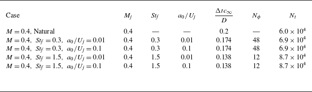

 ux′′

 u~x(ϕf)
 ϕf=0
 f=0
 u~x,0
 u~x(ϕf)=0.25,0.75
 u~x,0=0.25,0.75

 u~x,0
 σ(u~x)
 δθ

 (ux′′ux′′~)
 ϕf=0
 (ux′′ux′′~)0
 (ux′′ux′′~)
 ϕf=0, π/2, π, 3π/2
 Stf=0.3,a0/Uj=10%

 ux′′
 x=1.25, r=0.5
 x=5, r=0.5

 m^α(x,r)
 ux′′(x,r)
 α/α0=0
 α/α0=1
 α/α0=2

 E~(x,r,θ,ϕf)
 ϕf=0, (b)ϕf=2π/3
 (c)ϕf=4π/3

 E~r(x,ϕf)
 E~rx(x,ϕf)
 ϕf
 x
 E~rx(x,ϕf)
 [2, 10, 50, 90]% ×0.25

 E~rx,0(x)
 E~rx(x,ϕf)

 m=0
 Stf=0.3
 Stf=1.5

 m=0
 St=0.1
 Stf=0.3
 Stc=0.1
 ±0.75|ϕ(t)|∞
 u~x(ϕf)=0.25,0.75

 ±0.75|ψ(x,f)|∞

 m=0
 Stf=0.3
 Stc=0.05
 Stc=0.15
 ϕf=0
 ±0.75|ϕ(ϕf=0)|∞
 u~x(ϕf=0)=0.25,0.75

 m=0
 Stf=1.5
 Stc=0.05
 Stc=0.15
 Stc=0.475
 Stc=0.75
 ϕf=0
 ±0.75|ϕ(ϕf=0)|∞
 u~x(ϕf=0)=0.25,0.75

 Stf=0.3
 Stf=1.5
 m=1,2

 m=0
 Stf=0.3
 Stc=0.05
 Stc=0.15
 ϕf=0
 ±0.75|ϕ(ϕf=0)|∞
 u~x(ϕf=0)=0.25,0.75

 m=0
 Stf=1.5
 Stc=0.05
 Stc=0.15
 Stc=0.475
 Stc=0.75
 ϕf=0
 ±0.75|ϕ(ϕf=0)|∞
 u~x(ϕf=0)=0.25,0.75

 Stc,f=0.1
 ϕf=0
 (Stf=0.3)
 (Stf=1.5)
 ±|ϕ(ϕf=0)|∞
 u~x(ϕf=0)=0.25,0.75

 m=1
 m=2
 Stf=0.3
 Stc=0.05
 Stc=0.15
 ϕf=0
 ±0.75|ϕ(ϕf=0)|∞
 u~x(ϕf=0)=0.25,0.75

 m=1
 m=2
 Stf=1.5
 Stc=0.05
 Stc=0.15
 Stc=0.475
 Stc=0.75
 ϕf=0
 ±0.75|ϕ(ϕf=0)|∞
 u~x(ϕf=0)=0.25,0.75

 m=0
 Stc=0.1, α0=0.3
 ±0.75|ϕp(t)|∞
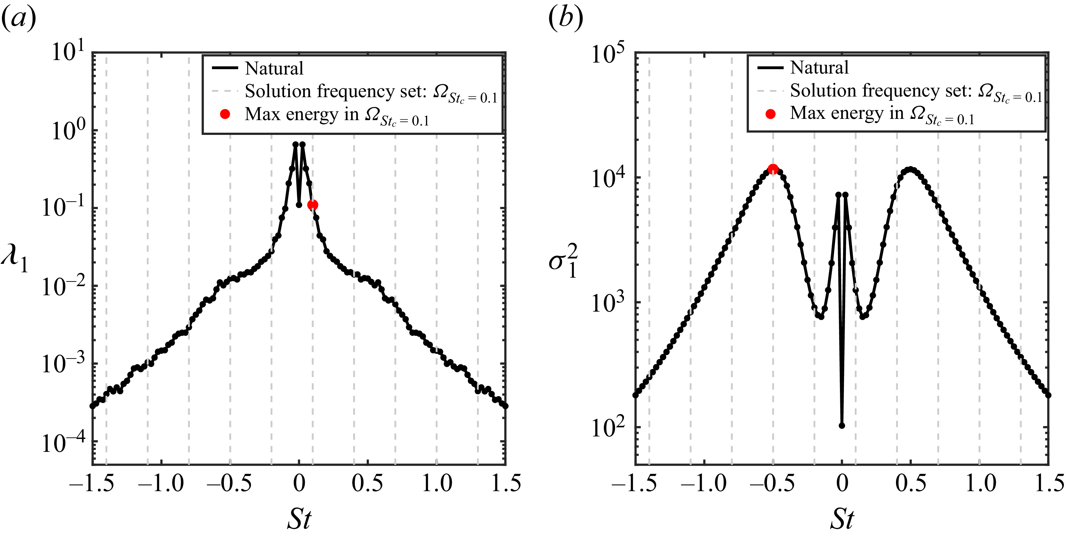
 Stc=0.1
 ΩStc


