INTRODUCTION
Based on permafrost studies as a scientific discipline, studying the permafrost must involve both glacierized and glacier-free areas, whereas areas under sub-freezing conditions within the glacier system tend to be studied from the glaciological point of view. Thus, glaciers and their surrounding environments tend to be studied as independent elements, precluding from any comprehensive analysis at the full glacier landscape scale from the permafrost perspective. Consequently, any research involving glacier–permafrost relations should be tackled from both the glaciology and the permafrost point of view. To this end, understanding the differences in the study of permafrost from these two disciplines is essential to establishing underlying research assumptions and the reasons behind study designs. Here, we analyse the glacial ice and periglacial areas of the Storglaciären, northern Sweden, to identify how a holistic (cryospheric) approach to glacier and permafrost studies can help us understand the relationship and evolution of glacier–permafrost system.
Traditionally, glaciology deals with all forms of frozen water found in nature (Shumskii, Reference Shumskii1964; Kotlyakov, Reference Kotlyakov1984; Martini et al., Reference Martini, Brookfield and Sadura2001; Paterson, Reference Paterson2002). Thus, Knight (Reference Knight2011:440) broadly defines glaciology as the “scientific study of ice in all its forms.” On the other hand, permafrost is defined by the International Permafrost Association (IPA, http://ipa.arcticportal.org/resources/what-is-permafrost.html [accessed March 6, 2017]) as any “ground (soil or rock and included ice or organic material) that remains at or below 0°C for at least two consecutive years” (cf. Everdingen, Reference Everdingen1998). The fact that glaciers and ice sheets partly or entirely consist of ice at sub-freezing temperatures is blatantly obvious, to the end that early studies even claim that glaciers are permafrost by definition (Muller, Reference Muller1943). Washburn (Reference Washburn1973) also supported this approach, together with Embleton and King (Reference Embleton and King1975), and King (Reference King1984), who believed that glaciers are only conventionally excluded from the permafrost definition but with no solid scientific reason. From our perspective and for the purpose of this study, it is important to emphasise both disciplines deal with ice and permafrost, which occur in both glacial and periglacial environments.
Very frequently, glacier and periglacial studies are independent from each other. In fact, while areas continuously covered by ice are considered glacial environments (glaciers, ice caps, and ice sheets), permafrost tends to be defined based on its temperature and durability over time (Everdingen, Reference Everdingen1998). Consequently, glaciers are defined as a material structure, while permafrost is a state, rather than a material structure, an invisible phenomenon, a specific ground thermal condition (Black, Reference Black1954, Reference Black1976; Haeberli et al., Reference Haeberli, Hallet, Arenson, Elconin, Humlum, Kääb and Kaufmann2006; Dobiński, Reference Dobiński2011a, Reference Dobiński2011b).
Hence, glaciers are defined materially, through the actual presence of ice, whereas periglacial environments are areas characterized by frost action and permafrost occurrence (Brodzikowski and van Loon, Reference Brodzikowski and van Loon1991). In this context, the term “periglacial environment” refers to cold-climate non-glacial processes and features regardless of their proximity to glaciers (Washburn, Reference Washburn1973; Jahn, Reference Jahn1975; French, Reference French2007). Permafrost occurrence is sometimes referred to as “underground glaciation” (Shumskii, Reference Shumskii1964; Jahn, Reference Jahn1975), which directly links to the research scope of glaciology. Actually, the core of periglacial geomorphology concerns the study of the freezing process, associated ground ice structures, and related landforms. It embraces a mix of glacial, periglacial, and azonal processes and identifies distinct characteristics common to all cold non-glacial regions of the world (French and Thorn, Reference French and Thorn2006; French, Reference French2007).
In practice, there is a clear gap between glacier and permafrost research, either by tradition or arising from the fact that glaciers are considered as a part of the hydrosphere and permafrost of the lithosphere (Shumskii, Reference Shumskii1964; Kneisel, Reference Kneisel1999; Lilleøren et al., Reference Lilleøren, Humlum, Nesje and Etzelmüller2013). This discrepancy represents the most substantial barrier to a holistic approach to cryospheric studies, limiting our comprehensive understanding of the link between glaciology and periglaciology/permafrost science.
The objective of this work is not to deliver basic information on the glacial and periglacial environments studies from the permafrost perspective; instead, we propose a uniform understanding of both systems. We use the well-known Storglaciären glacier, in the Tarfala Valley in northern Sweden, to illustrate the level of structural complexity found in glacier–permafrost systems. Storglaciären is internationally recognised as a “glaciological laboratory” for the scientific community, and the Storglaciären forefield has been subject to extensive permafrost and periglacial research. Permafrost occurrence in the Tarfala area and the presence of ground ice forms (e.g., ice cored moraines) has been thoroughly investigated (e.g., Østrem, Reference Østrem1964; King, Reference King1984, Reference King1986; Kneisel, Reference Kneisel1999, Reference Kneisel2003; Marklund, Reference Marklund2011).
We also aim to improve our understanding of the links between ice occurrences, especially of glacial ice, and the presence of permafrost in both glacial and periglacial environments in mountainous areas by identifying the geophysical characteristics of the glacier–permafrost complex. Therefore, here we focus on a cryotic system including a polythermal glacier and permafrost on forefield, from a region with a variable yet continuously favourable cold climate. Frost penetration appears as a physical process common to both glacial and permafrost environments, encompassing them to a different extents. The advantage of this approach includes the possibility to conduct combined glacial and periglacial studies, as well as unifying the research approach by considering both environments as components of the lithosphere.
PREVIOUS STUDIES AND RATIONALE
There is not an obvious first study on glacier–permafrost relations identified as the pioneer in the field and, indeed, integrated glacier/permafrost studies have been repeatedly attempted for several decades (see e.g., Shumskii, Reference Shumskii1964; Haeberli, Reference Haeberli2005). For example, Waller and Tuckwell (Reference Waller and Tuckwell2005) claimed that the interaction between glaciers and permafrost has been considered unimportant until recently because cold-based glaciers have been assumed to be geomorphologically ineffective; in addition, numerical ice-sheet models suggest that glacier–permafrost interactions are limited in extent, and restricted to the marginal fringes of ice masses. The first book devoted to this issue was published by Harris and Murton (Reference Harris and Murton2005a), and the subject was most recently reviewed by Waller et al. (Reference Waller, Murton and Kristensen2012).
The specificity of glacier freezing is particularly evident in the glacier’s thermal structure (Blatter, Reference Blatter1990). In fact, the presence of permafrost in glaciers has been repeatedly described (Björnsson et al., Reference Björnsson, Gjessing, Hamran, Hagen, Liestol, Palsson and Erlingsson1996; Etzelmüller and Hagen, Reference Etzelmüller and Hagen2005: figs. 1 and 2). Hughes (Reference Hughes1973) was the first to use the term “glacial permafrost” in a material context, while Dobiński (Reference Dobiński2011a, later developed in Dobiński [Reference Dobiński2012]), referred to glacier permafrost in the context of glacial ice.
We can currently consider the debate on glacier–permafrost relations as developing two main research directions: the first, and the dominating one, considers permafrost as a “material concept.” In particular, this research line deals with issues such as: (1) glaciotectonic processes, (2) ground-ice development, (3) rock glaciers, (4) proglacial and ice-marginal processes, and (5) permafrost and related processes (Harris and Murton, Reference Harris and Murton2005a, Reference Harris and Murton2005b; Waller et al., Reference Waller, Murton and Kristensen2012). The other direction, which may be labelled “geophysical,” revolves around the identification of the glacier–permafrost relation based on basic characteristic of the permafrost, i.e., a temperature (state) of ≤0°C. In this case, the “geophysical” approach tends to deal with the process of frost penetration and its occurrence in the glacier and its forefield (Kneisel, Reference Kneisel1999, Reference Kneisel2003; Pettersson et al., Reference Pettersson, Jansson and Holmlund2003, Reference Pettersson, Jansson and Blatter2004; Petterson, Reference Pettersson2004; Etzelmüller and Hagen, Reference Etzelmüller and Hagen2005; Dobiński, Reference Dobiński2011a, Reference Dobiński2011b, Reference Dobiński2012; Dobiński et al., Reference Dobiński, Grabiec and Gadek2011).
The first research direction, in particular, investigates ice as a part of the extraglacial environment and associated processes. The second direction, on the other hand, essentially concentrates on one particular process, i.e., frost penetration and its spatial distribution, directly related to its temperature and physical parameters of the study medium, depending on whether it is frozen or not.
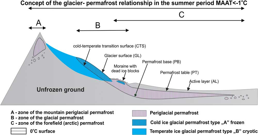
In principle, permafrost studies exclude glaciers. As a result, ice is perceived sometimes as an “additional component” (Dobrowolski, Reference Dobrowolski1953), belonging neither to the hydrosphere nor the lithosphere. Thus, incorporating glaciers into the lithosphere arises as an essential precondition for conducting comprehensive cryosphere/permafrost studies. Considering permafrost as a geophysical phenomenon allows identifying it within both periglacial and glacial environments. This approach also allows solving any issues associated with the relation between glaciers and permafrost, as the concept of glacial permafrost developed by Dobiński (Reference Dobiński2011a, Reference Dobiński2011b, Reference Dobiński2012). Dobiński (Reference Dobiński2011a) identified an environmental axis along the cold-temperate transition surface (CTS), turning into the permafrost base (PB) in glacier forefields of polythermal glaciers (Dobiński et al., Reference Dobiński, Grabiec and Gadek2011). This approach also allows identifying and studying permafrost as part of both glacial and periglacial environments (Fig. 1). This model can be defined as the CTS-PB model and used as an approach, albeit it provides a static and overly simplistic image of the system, particularly when complex glacier dynamics are considered, e.g., glacier surges or transgressions over a permafrost area. However, this simple solution is still useful to conduct holistic studies including the glacial–periglacial interface, as long as these static assumptions are considered during data interpretation. For example, the CTS-PB axis is essential to understand the thermal evolution of polythermal glaciers and permafrost on their forefields, which are difficult to put together using solely geophysical methods, as is still occurring in this field of research.
(color online) Glacier–permafrost interaction as a general relation between surfaces whose temperature remains close to 0°C (CTS-PB). This layer permanently exists at the bottom of the glacier and along the permafrost, integrating glacial and periglacial environments from the geophysical point of view, updated after Dobiński (Reference Dobiński2006, Reference Dobiński2012).

GEOGRAPHICAL SETTINGS
The Tarfala Valley (Fig. 2) and its surroundings represent the highest region of the northern Scandinavian Mountains and include the Kebnekaise, the highest mountain in Sweden reaching 2117 m asl. Its peak is covered throughout the year by a small body of snow and subfreezing ice. Storglaciären (67°55'N, 18°35'E) is on the eastern flank of the Kebnekaise ridge. The mean annual air temperature (MAAT) over the period 1965–2011 was –3.5°C at the nearby Tarfala Research Station (1135 m asl; Jonsell et al., Reference Jonsell, Hock and Duguay2013) and the mean annual precipitation is approximately 1997±450 mm (Dahlke et al., Reference Dahlke, Lyon, Stedinger, Rosqvist and Jansson2012). The summer lapse rate is 0.7°C/100 m, whereas the winter lapse rate is –0.6°C/100 m, as a consequence of lower winter temperatures in the Ladtjovagge valley compared to Tarfala. The valley bottom is a mix of bare rocks, grasses, mosses, and lichens. Dwarf shrubs, mainly species belonging to the genus Salix, appear up to 1000 m asl and the birch forest reaches up to 700–750 m asl (Fuchs, Reference Fuchs2013). The Kebnekaise massif is made of hard slates, granites, gneiss, amphibolites, and peridotes. Its overall geomorphology mainly results from a long-lasting glaciation process, leading to the creation of a high-mountain environment with all its characteristic components.
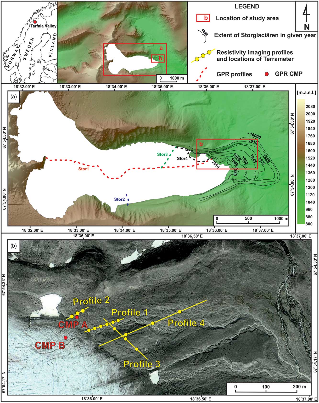
(color online) Location of the research area in Kebnekaise, Northern Sweden. (a) Dashed lines represent the GPR profiles. Glacier retreat marked as solid lines. (b) Resistivity imaging profiles (ERT; mapdata: Google, DigitalGlobe). CMP A, common mid-point measurements on the forefield; CMP B, common mid-point measurements on the glacial ice. Digital Terrain Model courtesy of the Tarfala Research Station.

Early permafrost studies in the Kebnekaise massif were conducted by Østrem (Reference Østrem1964), who use geophysical methods to study ice-cored moraines. Similar work was undertaken by King (Reference King1984, Reference King1986), who defined permafrost zonation for northern Scandinavia. King (Reference King1984, Reference King1986) set the limit of sporadic discontinuous permafrost occurrence at 750 m asl and 1200 m asl for discontinuous permafrost. Continuous permafrost, on the other hand, starts above 1500 m and it can reach thickness of over 100 m. In fact, in the nearby Tarfalaryggen (67°55'09''N, 1540 m asl), permafrost thickness is estimated to be 350 m (Harris et al., Reference Harris, Haeberli, Vonder Mühll and King2001; Isaksen et al., Reference Isaksen, Holmlund, Sollid and Harris2001). Studies on permafrost conducted by Kneisel (Reference Kneisel1999, Reference Kneisel2003) show that permafrost also occurs locally in the central parts of the glacier forefield, in some higher locations and along the former maximum extent margin (reached in 1910).
Storglaciären is a polythermal valley glacier covering ca. 3.1 km2 with an annual mean temperature of approximately –6.0°C at the average equilibrium line altitude (1469 m asl). The glacier is surrounded by continuous permafrost, except at the forefield, where the permafrost is discontinuous (Isaksen et al., Reference Isaksen, Holmlund, Sollid and Harris2001; Holmlund et al., Reference Holmlund, Jansson and Pettersson2005). The average thickness of Storglaciären is 95 m and the maximum thickness is 250 m (Jansson, Reference Jansson1996). The glacier has been steadily retreating since 1910, when it reached its maximum extent (Holmlund et al., Reference Holmlund, Jansson and Pettersson2005). Its dynamics and hydrology were reviewed by Jansson (Reference Jansson1996). In addition, Holmlund et al. (Reference Holmlund, Jansson and Pettersson2005) analyzed 58 years work of mass balance data, while Petterson et al. (Reference Pettersson, Jansson and Holmlund2003) published a study on its polythermal structure.
METHODS
Geophysical methods carry the advantage of being able to precisely distinguish between frozen and non-frozen materials of periglacial environments, and between “temperate” and “cold” ice of glacial environments, as the physical characteristics of these materials change significantly along their phase transitions. However, permafrost may be partially frozen or unfrozen (cryotic) at 0°C when it is under pressure, mineralised, or when the medium is highly fine-grained. Bearing in mind that the thermal characteristics of Storglaciären and the occurrence of permafrost on its forefield have already been well-defined by other authors (Østrem, Reference Østrem1964; King, Reference King1984, Reference King1986; Kneisel, Reference Kneisel1999, Reference Kneisel2003), here we use methods known to be well fit to illustrate the relation between the polythermal glacier and the permafrost on its forefield.
Ground penetrating radar
This method uses radio waves to identify boundaries between elements of contrasting dielectric properties. This method also allows defining those properties. Ground penetrating radar (GPR) is widely used both for glacial (e.g., Plewes and Hubbard, Reference Plewes and Hubbard2001) and periglacial research (e.g., Moorman et al., Reference Moorman, Robinson and Burgess2003). To this end, temperature can influence significantly the physical properties of the medium studied using GPR; for example, the dielectric properties of water depend directly on its state, which, in turn, depends on temperature.
Water shows a high relative permittivity (k) in liquid state (k=81) while that of ice depends on its density and ranges between 3 and 4 (lower k values are found in snow due to the presence of air). Ice is also characterised by a low attenuation coefficient. In contrast, liquid water strongly absorbs and diffuses waves in the typical spectrum used for glacier GPR surveys. Due to the difference in relative permittivity between liquid and frozen water, GPR can be very useful to distinguish between frozen and unfrozen materials, allowing to properly identifying the thermal condition of the ground. The reflection coefficient shows how much energy is reflected at the boundaries and how much is transferred through. It derives from the relative permittivity of the materials at the structural boundaries, and its absolute value increases with the increase in the differences between dielectric properties (Neal, Reference Neal2004). As a consequence, GPR is a good tool to distinguish between layers saturated with water (e.g., the active layer of permafrost) and those containing ice of glacial (e.g., ice core) or periglacial (e.g., congelation ice) origin, by identifying boundaries between them based on high absolute reflection coefficients. However, we are also aware of the issues arising from using GPR on porous media, which could be dry (frozen), wet, or presenting a combination of both.
We conducted a GPR survey across the complex of glacial and periglacial environments associated with the Storglaciären glacial system, using an impulse radar and unshielded 200 and 100 MHz central frequency antennas. The GPR measurements were taken using both the common offset mode, useful to obtain a 2-D image of the subsurface structure along the profiles, and the common midpoint (CMP) mode, useful to define the dielectric properties of each individual soil layer (relative permittivity and radio wave velocity, RWV). In total, the common offset profiles covered 7.63 km, and 83% of the data were collected using the 100 MHz antenna. The radar pulses were generated with 0.2 s interval (200 MHz antenna) and 0.5 sec (100 MHz antenna), which meant a record of ca. 11 and 3 traces/m, respectively. We also gathered GPS position data simultaneously, using a kinematic differential GPS receiver to geographically locate the profiles. The staff at the Tarfala Scientific Station provided the reference GPS data. The average accuracy of the DGPS positions was: 0.18 m for the X and Y axes and 0.53 for the Z axis. The GPR traces were subsequently linked to their GPS coordinates and processed using DC removal, time-zero adjustment, running average subtraction, bandpass filtering, and signal gain.
In addition, CMP measurements were taken from two locations representative of the glacier and its forefield (Fig. 2). Both CMP profiles were gathered parallel to the glacier front using the 200 MHz antenna and at 0.6 m intervals between individual antenna positions. The length of each profile was 30 m.
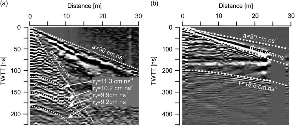
The geometry of the lines connecting amplitude anomalies in a series of traces (Fig. 3) makes it possible to define RWV for each individual layer, and to determine the dielectric properties of these media. The shape adjustment of model lines defining reflective surfaces was performed 10 times, and the mean values of RWV and the relative permittivity of the layers were calculated to obtain the standard deviation of the results, which was treated as an indicator for possible errors during parameter evaluations.
Results of the GPR common mid-point (CMP) survey on the moraine material on the forefield (a) and (b) on the glacial ice. RWV, layers ranging between surface and depths are marked by dotted lines in both environment; TTWT, two way travel times of radar signal (ns).

The CMP data provide essential information to convert the GPR data from a time scale into a depth scale. Additionally, the dielectric properties determined as described above allow for a more reliable interpretation of the characteristics (e.g., lithology, porosity, and water content) of the probed material.
Electrical resistivity tomography
Two-dimensional direct current (DC) resistivity tomography, also known as ERT or Electrical Resistivity Imaging (ERI) in 2-D, is a useful tool for permafrost research, allowing investigation of underground structures, properties, and spatial diversification of the permafrost in a non-invasive manner (Isaksen et al., Reference Isaksen, Hauck, Gudevang, Ødegård and Sollid2002; Hauck et al., Reference Hauck, Isaksen, Vonder Mühll and Sollid2004; Kneisel et al., Reference Kneisel, Hauck, Fortier and Moorman2008; Hilbich et al., Reference Hilbich, Marescot, Hauck, Loke and Mausbacher2009; Yanhui et al., Reference Yanhui, Qihao, Xicai, Xinbin and Lei2013).
The geological medium is hardly ever homogeneous, and this heterogeneity is reflected in changes in electrical resistivity of the medium. By measuring electrical resistivity using several electrodes spaced across the surface of the study area, we can identify sub-surface structures (Hauck and Kneisel, Reference Hauck and Kneisel2008; Loke, Reference Loke2014).
Similarly to GPR, ERT does not incorporate temperature measurements; however, the presence of ice can be identified as high resistivity values in the ground. In fact, the resistance of glacial ice can reach values up to 108 Ωm (Reynolds, Reference Reynolds1997). In geological media, electric charge transport mainly happens through ionic conduction. Therefore, rock water content, water mineralisation, and water flow capacity are the main factors influencing electrical resistivity. Thus, the occurrence of ice within soil pores in permafrost plays a key role determining the phase transition of water around 0°C. Depending on its proportional volume, the bedrock type, pore type, and water saturation within pores, permafrost resistivity can range from few kΩm to MΩm (Hoekstra and McNeill, Reference Hoekstra and McNeill1973; Marescot et al., Reference Marescot, Loke, Chapellier, Delaloye, Lambiel and Reynard2003). In fact, ERT might not provide satisfactory results for ice-free permafrost.
Here, we used an ABEM Terrameter LS to conduct the ERT surveys along 4 profiles (Fig. 2). In this case, we spaced the electrodes by 1, 2.5, and 5 m, which provided maximum penetration depths of ca. 15, 40, and 75 m, respectively. Increasing the penetration depth decreases the resolution of the resistivity data collected, justifying the use of different electrode spacing.
During DC resistivity surveys, most of the electrode must be in direct contact with the ground. This is not always feasible since the surface of the glacier forefield presents thick moraine deposits, including boulders with interstitial voids filled with air, water, and clay. This ground structure explains the very high variability showed by the resistance data collected during the contact test. These values ranged from 5 kΩm to 260 kΩm depending on the surface structure of the place where the electrodes were located on the ground. As a result, most measurements relied on only weak currents. In the case of the profiles with 1 m electrode spacing, we added some silt collected from a nearby stream to improve electrode-ground contact. For the profile surveyed using electrodes spaced 2.5 and 5 m, the electrodes could be placed in a more convenient spot, i.e., at a distance of ca. 20 cm from the planned site, perpendicular to the measurement profile. The level of error from this approach is known to be not significant (Zhou and Dahlin, Reference Zhou and Dahlin2003), allowing some flexibility at the time of placing the electrodes. Only 19 and 24% of the measurements made using the Schlumberger method used a current over 5 mA for Profiles 1 and 2, respectively, due to the placement issues described above. These percentages increased to 63 and 58% for Profiles 3 and 4, respectively.
All electrode positions were recorded using a Leica GPS in the differential static mode. The mean accuracy of the horizontal position was 0.02 m, while the average vertical accuracy was 0.05 m. The Schlumberger electrode array has been used for this type of measurement, and it has been shown to return a good balance between signal strength and spatial resolution (Dahlin and Zhou, Reference Dahlin and Zhou2004; Loke, Reference Loke2014).
The data were subsequently processed using Res2Dinvx64 v.4.0. In the standard version of the software, data processing is based on the smoothness constrained least squares method. During data inversion, we tested various parameters for each profile to find the best fit data processing methodology which could be homogeneously used for all profiles. As the level of noise was high due to the weak signal used, the least squares method did not return satisfactory results. For this reason, we used the absolute difference method, which minimises the difference of the first power between the measured and the estimated apparent resistivity (Olayinka and Yaramanci, Reference Olayinka and Yaramanci2000; Loke et al., Reference Loke, Acworth and Dahlin2003; Loke, Reference Loke2014). Moreover, implementing the L1 standard to minimise resistivity changes in the model generated unrealistic results, which tended to reduce resistivity anomalies. Hence, we applied the conventional smoothness-constrained least squares method. Additionally, each data set was tested individually to find the best results to identify horizontal structures and how they responded to different damping factors. These tests did not return considerable differences among most models, supporting the final choice of the Res2Dinv settings. We used the model refinement option for the Profiles 1 and 2, to increase the degrees of freedom of the models, as these profiles showed a considerable variability in resistivity at the surface. The convergence limit was set to a 5% error difference in relative change between two iterations, to reduce the model artificial tendency to overfit the data, thereby demonstrating an increase in existing resistivity contrasts. This error level was appropriate for both the measured data itself and the inversion routine. For most cases, the inversion stopped between the fifth and the seventh iteration.
RESULTS
The GPR survey was particularly aimed to identify the structure of the glacier whereas the ERT was specifically used on the non-glacierized forefield.
Dielectric properties of the glacial–periglacial Storglaciären complex
The CMP measurements taken on the glacier forefield show a multilayered ground structure with different properties (Fig. 3a). The near-surface layer is characterised by dielectric parameters typical of till saturated with water. The layer down to ca. 6.5 m shows a relatively low relative permittivity (k=7.05), and therefore, it is possibly made of glacial till or rock waste. These formations are desiccated or contained very little water. RWV of 5.8–7.7 cm/ns suggests that the subsequent layers were sediments of glacial origin saturated with water. The dielectric properties of the media down to ca. 8.4 m deep do not show evidences of underground ice.
In the case of non-glacierized areas, the time-to-depth scale conversion was based on a RWV of 10 cm/ns. This is the average value estimated for the till layer, obtained using CMP down to a depth of ca. 7.5 m.
The structure in the CMP profile taken at the glacial margin of Storglaciären (Fig. 3b) appears to be much more homogenous. It comprises two layers: an upper layer with the properties of cold ice and a lower glacial base. The speed of the ground wave suggests the presence of pure ice (i.e., 16.8 cm/ns) despite a substantial amount of water on the glacial surface. The base lies at a depth of 15.78±0.36 m and is outlined in the profile as a distinct reflection. RWV within the glacier is relatively low for cold ice (15.8±0.32 cm/ns), suggesting the presence of considerable amounts of moraine material incorporated into the glacier and high water content. We used RWV of 15.8 cm/ns to convert the time scale into a depth scale for the glacial ice profiles.
Materials composing the Storglaciären glacial system
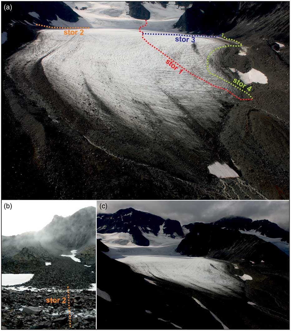
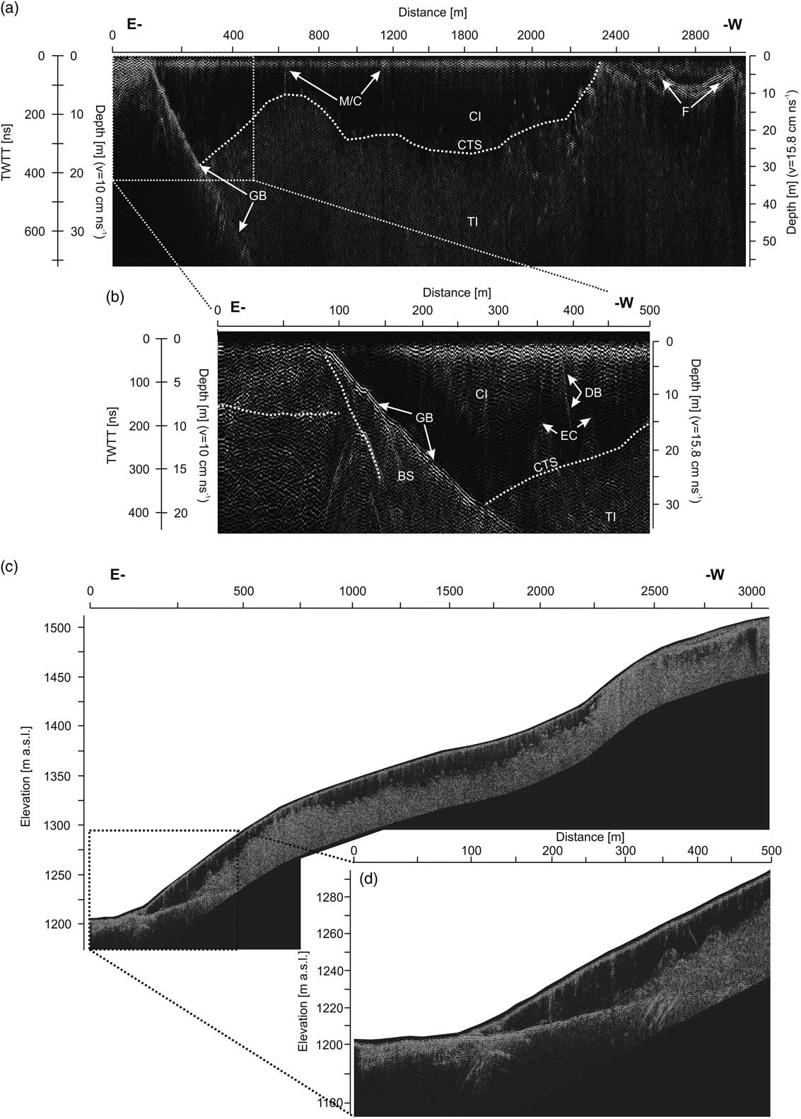
The longest GPR profile performed on the glacier (Stor 1) was 3070 m long (Figs. 2 and 4). We used this profile to identify the thermal structure of the glacier, its stratification, and the potential presence of till material within the glacier ice (Fig. 5). The profile starts on the forefield and runs along the glacial axis to the eastern edge of the Østkammen ridge. The first 90 m run on till material deposited on the forefield. The image structure reaches the depth of ca. 30 m. The clearest horizon is visible at the depth of ca. 13 m and starts at the glacial front. This horizon presents a relatively distinct reflection, which may indicate the presence of a water filled layer, till on a layer of buried ice, or bedrock (Fig. 5b and d). The glacier bed is visible on the GPR profile for ca. 470 m of the profile and ca. 56 m of depth (Fig.5a and c). However, numerous hyperbolic structures are also visible below the base line, suggesting some level of diffraction from the bottom material. A horizon running through the bed from the glacial front but falling more steeply than the glacial bottom was also apparent, and it may be interpreted as a decollement in the subglacial sediments (Fig. 5b and d; Dobiński et al., 2011). A distinct horizon in the base occurs between the glacial front and ca. 120 m of the profile at a depth of 14–19 m (Fig. 5b and d).
(color online) Overview of the GPR profiles on Storglaciären. (a) Location of all the profiles mentioned in the text and related to ice and moraine material. (b) Location of the profile Stor 3 on the slope/glacier interface. (c) General overview of Storglaciären and its forefield.

Longitudinal cross section of Storglaciären performed by GPR. (a) Entire length of profile Stor 1. (b) The first 500 m of the Stor 1 profile, showing a better contact between cold and temperate ice and the CTS contact with the bottom sediments/bedrock. (c and d) GPR profile similar to that in Figure 5 a and b put together overlying the glacier topography. In this case, structural boundaries are not marked for clarity. CI, cold ice; TI, temperate ice; CTS, cold-temperate transition surface; F, firn layers; EC, englacial conduits; M/C, moulin/crevasse; DB, debris band; GB, glacier bed; BS, bottom sediments; BI, buried ice; S-I, snow-ice patch; BRC, bedrock; TL, talus slope; IM, internal moraine; LM, lateral moraine; SM, superficial moraine; GS, glacier surface.

Up to ca. 260 m, the glacier is probably frozen to its bed (Fig. 5b and d). Further on, a layer of temperate ice appears in the lower part. The cold ice reaches its maximum thickness (ca. 30 m) in the areas with temperate ice at the bottom. From then on, cold ice thickness fluctuates between 0 and 30 m (Fig. 5a and c), and the cold ice layer thins out and disappears at ca. 2300 m from the glacier front, near the equilibrium line. Underneath, there is a multi-reflexive layer of temperate ice identified as wave diffractions from water bodies within the ice, which is at its pressure melting point. In the layer of temperate ice, shear plane and stratification related to sedimentation run parallel to the surface (Fig. 4a). There are also layers identified as firn over the equilibrium line. It is possible to distinguish a maximum of 4 such horizons. In some places underneath, stratification is visible, possibly indicating the presence of an irregular metamorphism rate (Fig. 5a and d).
The longitudinal profile of the glacier did not reach the glacial bottom over its entire length; however, it reflected very well the specificity of the thermal system of the bed, distinctly showing a two-layer structure. The upper cold-ice layer, with much lower water content, is the frost-penetrated layer. Underneath is the layer of temperate ice at the pressure melting point. These layers are separated by a CTS boundary. In the area of its main axis (except for the frontal area), the glacier presents low moraine material content. Higher sediment content is visible in places where the glacier front is frozen to the bed. As a result of compressive motion, moraine material is pushed onto the ice surface, forming a till sediment layer that partially covers the glacial front in the marginal zone (Fig 4a).
Southern lateral zone
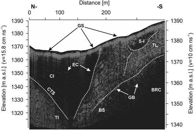
The Stor 2 profile runs from the centre of the glacier to its edge at the north-exposed slope (Figs. 2a and 4a). At a distance of ca. 150 m from the beginning of the profile, a two-layer structure of polythermal glacial ice is visible, where the thickness of the cold layer increases towards the glacial margin from ca. 20 m to ca. 56 m at the edge (Fig. 6). Then, between 235 and 280 m, there is an ice/snowfield, constituting the outer part of the glacier. The maximum thickness of this formation reaches ca. 13 m. Underneath there is probably ca. 1.5 m of sediments on a solid rock surface, which subsequently turns into a talus located on the non-glacierized slope. The terminal part of the profile (ca. 10 m) constitutes a steep talus slope, reaching a thickness of ca. 11 m at the profile end. This structure could arise as the talus-cone material covers the marginal part of glacial ice, as that part of the glacier, along with the slope, is largely in the shade and consequently cooler than its surroundings, facilitating ice preservation. This situation, however, is not reflected in the shape of the glacier or its topography, as shown in Figures 4a and b. As a result, the distinct internal moraine and the snow/ice-patch found along with the scree bound with ice is most probably deeply frozen, also forming part of the ice in the cold surface layer of the glacier. Our observations also suggest that the active layer of permafrost must be much thinner on this side of the glacier compared with the opposite slope. The boundaries between the glacial and periglacial environment are clear up to this point, when they become indistinct. This is because of the accumulation of rubble sediments from the surrounding slopes, which form the internal moraine further on as the glacial ice moves along (Fig 4).
Transverse GPR cross sections of the southern part of Storglaciären (profile Stor 2). Figure shows contact between the talus slope sediments, the glacier, a partially buried snow-ice patch and the bedrock. CI, cold ice; TI, temperate ice; CTS, cold-temperate transition surface; F, firn layers; EC, englacial conduits; M/C, moulin/crevasse; DB, debris band; GB, glacier bed; BS, bottom sediments; BI, buried ice; S-I, snow-ice patch; BRC, bedrock; TL, talus slope; IM, internal moraine; LM, lateral moraine; SM, superficial moraine; GS, glacier surface.

Northern lateral zone
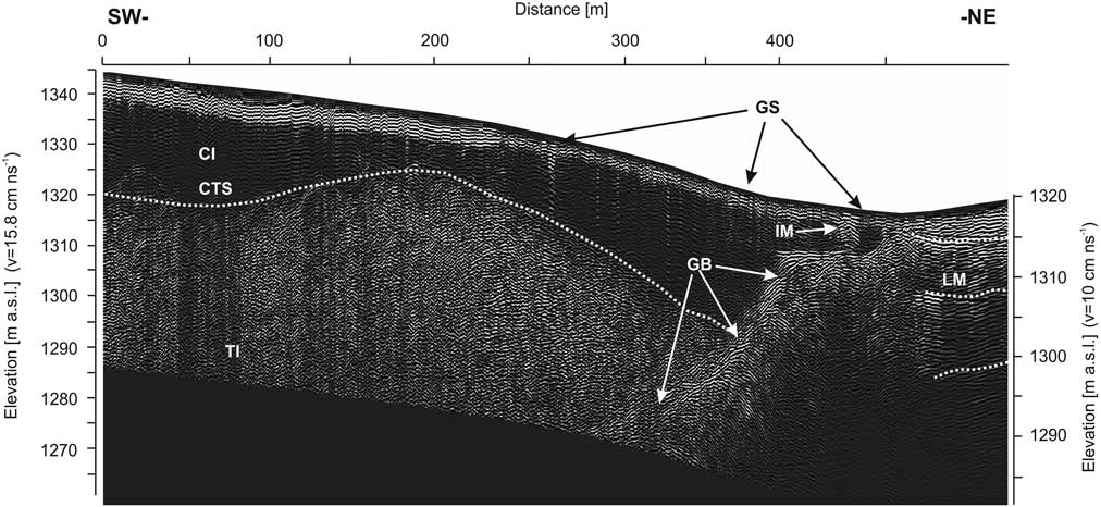
The counterpart of the Stor 2 profile on the opposite side of the glacier, from its axis to the south-exposed slope, is the Stor 3 profile (Figs. 2 and 4), which is 490 m long. The two-layer structure of the glacier is visible at ca. 380 m of this profile (Fig. 7). The thickness of the cold ice ranges from ca. 22 m at the beginning of the profile, through ca. 13 m at ca. 200 m, to ca. 27 m at the 380 m area. Further on, cold ice is adjacent to the bottom and thins out towards the glacial edge. The base is visible on the profile from ca. 340 m and ascends steeply towards the edge. From the 415 m point of the profile, the base settles at a depth of ca. 10 m, forming a shelf ca. 25 m wide. The glacial surface over that shelf is covered with debris that hinders ice identification. At ca. 432 m of the profile, a multi-reflexive structure is visible within the glacier, suggesting the presence of an internal moraine built of clastic material bound by ice. From 455 m, the profile runs on till material and from 470 m it ascends along the lateral moraine. In this zone, a reflexive horizon is visible at the depth of ca. 2 m (a k coefficient different from what is assumed for ice). This might be associated with the thickness of the active layer of permafrost; however, this horizon seems to be a continuation of the glacial bottom, meaning that this boundary could also represent a structural feature. Below, horizons are visible at depths of c. 12 and 20 m, suggesting that the moraine has an ice core. The determination of the boundary between the glacial and periglacial environment is difficult on this side of the glacier, as the glacial surface is covered with slope material, which is incorporated into the glacier body where in some places takes the shape of an internal moraine.
Transverse GPR cross section of the northern part of Storglaciären (profile Stor 3). The margin of the glacier is unclear, although it is a visible contact between the glacial ice and the lateral and internal moraines. CI, cold ice; TI, temperate ice; CTS, cold-temperate transition surface; F, firn layers; EC, englacial conduits; M/C, moulin/crevasse; DB, debris band; GB, glacier bed; BS, bottom sediments; BI, buried ice; S-I, snow-ice patch; BRC, bedrock; TL, talus slope; IM, internal moraine; LM, lateral moraine; SM, superficial moraine; GS, glacier surface.

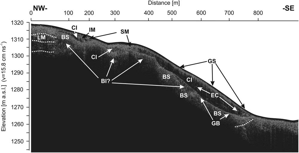
The Stor 4 profile also presents a considerable volume of slope material and glacial ice, similar to that described for the terminal parts of the Stor 2 and Stor 3 profiles (Fig. 8). This profile enables a comprehensive view of the diversification of slope sediments and glacial structures over a relatively large distance (900 m) within the ice tongue. In this case, the marginal zone is covered with a thick layer of till turning into slope sediments. The first 48 m of the profile run over the slope of a lateral moraine. Further on, in the marginal zone of the glacier and under the till material, there is a layer of ice reaching ca. 10 m. In the zone between the lateral moraine and up 155 m of the profile, the ice lies on a sediment layer. Below there is a structure similar to an ice core of ca. 15 m thick (RWV= 15.8 cm/ns). Between 260 and 390 m, the profile runs across the medial moraine, forming a conglomerate of ice and debris. After descending the bank of the medial moraine (360 m), the profile runs downwards following the lateral side of the glacier. Subsequently, the ice thickness increases to ca. 21 m at ca. 620 m of the profile and, further on, it thins out towards the glacial front (780 m). At this point, the bottom seems to be composed of soft sediments rather than bedrock. The most striking structure within this section is an ellipsoidal reflection at a depth of 10–18 m between 500 and 580 m. This structure could represent a depression filled with ice lying on sedimentary material. In the frontal zone, between 750 and 790 m, there is a steeply descending horizon similarly to the structure found in the frontal zone of the Stor 1 profile.
Lateral zone and moraine on the northern part of the glacier profile Stor 4. Relation between ice and sediments of different genesis is visible. CI, cold ice; TI, temperate ice; CTS, cold-temperate transition surface; F, firn layers; EC, englacial conduits; M/C, moulin/crevasse; DB, debris band; GB, glacier bed; BS, bottom sediments; BI, buried ice; S-I, snow-ice patch; BRC, bedrock; TL, talus slope; IM, internal moraine; LM, lateral moraine; SM, superficial moraine; GS, glacier surface.

The GPR profile shows a difference between ice and sedimentary materials originating from the surrounding slopes and subsequently transported on and into the glacier. The glacial bed topography and the englacial thermal structure, in relation to ice types and mineral components, are also apparent in the GPR profiles.
Composition of the periglacial glacier forefield
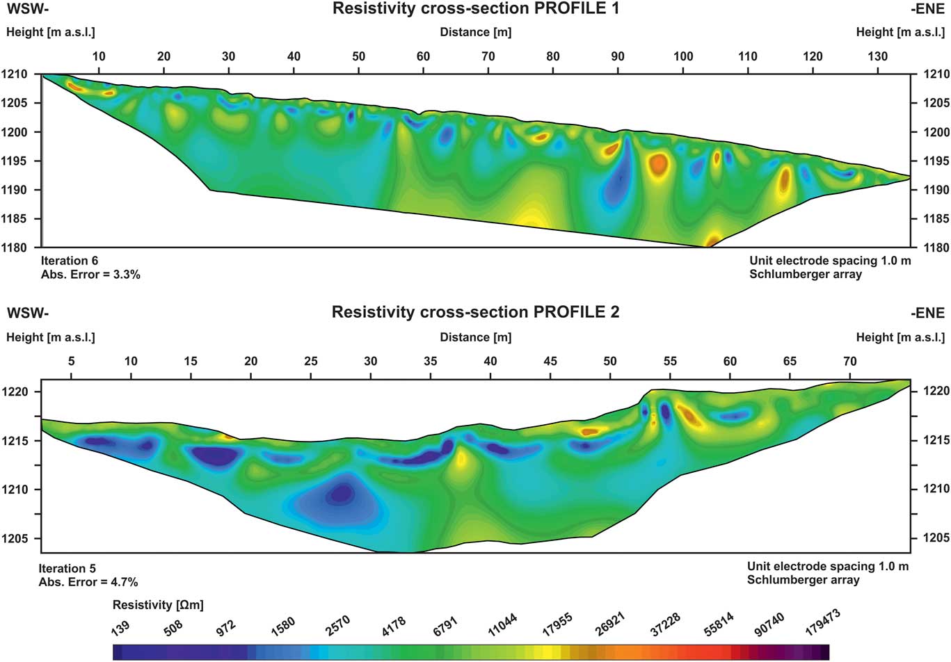
ERT data were collected from 4 profiles 140 m (Profile 1), 80 m (Profile 2), 200 m (Profile 3), and 400 m (Profile 4) long, located along the glacier forefield (Fig. 2b). In addition, data from two shorter and shallower ERT profiles (Profiles 1 and 2) were collected near the glacier front, to confirm the occurrence of the contemporary climate-related permafrost previously described for the glacier forefield (King, Reference King1984, 1986; Kneisel, Reference Kneisel1999; Marklund, Reference Marklund2011; Fuchs, Reference Fuchs2013). The ERT data taken using wider electrode spacing (Profiles 3 and 4) were used to verify the presence of a deeper lying permafrost layer, and to collect information regarding its evolution.
Area of intense surface and underground drainage
Profile 1 started directly on the forefield of glacial front (Fig. 2b). This area is water saturated and dominated by fresh till sediments of variable fraction. Small spacing between electrodes (1 m) allowed reaching depths down to ca. 15 m using the Schlumberger configuration. The profile shows a series of highly resistive near-surface anomalies, increasing in number and depth range down the slope, with the increase in distance from the glacial front (Fig. 9). This non-homogeneous layer reaches the depth of ca. 1 m. This layer is identified as un-frozen and relatively dry material filled with air, with resistivity values ranging 10–20 kΩm. Underneath, in the vicinity of the glacial front, another discontinuous layer appears, with a much lower resistivity, of the range 1–4 kΩm. This layer reaches a depth of 2–3 m; subsequently, highly resistive larger anomalies reappear, where the resistivity strongly exceeds 10 kΩm. The layer of low resistivity is identified as section of the active layer containing glacial till and saturated with water. Water drainage into the lower sediment is partly precluded by the layer of permafrost located underneath. This permafrost layer is discontinuous, probably due to degradation by an outflow of ablation water. This affects the resistivity of the media at this point, which weakly exceeds 20 kΩm. The high-resistive anomaly again reappears at the bottom of the lower part of the profile. It is possible that at this depth (10–13 m), we are indeed detecting the bedrock, which could from these data be in a frozen state.
(color online) Shallow ERT profile on the wet forefield found at the glacier terminus (Profiles 1 and 2). Permafrost resistivity values are much lower as this zone is at its initial state, with a relatively low thickness, probably of a discontinuous character and with liquid water.

The second profile (Fig. 9) was longer, extending over 80 m, and surveyed using an electrode spacing of 1 m. This profile followed a small depression in the northeastern part of the glacier forefield, near a perennial snow patch. There was a visible outflow from the snowfield and the glacier surface in this area. The upper layer of the profile is constituted by till not saturated in water. The younger part of this section is located near the glacier, ca. 60 m from the profile. The older, drier, and frequently less steep section appears ca. 42 m towards the beginning of the profile. The resistivity inside this area ranged within 10–15 kΩm on average. Low resistive anomalies are apparent directly beneath the surface, with resistivity values dropping as low as 1–2 kΩm. Subsurface outflow probably occurs in these sites. Below, at the depth of 3–5 m, there is another uneven discontinuous layer approximately 2–3 m thick, where the resistivity values range from ca. 4 kΩm near the glacier, to 15 kΩm in the forefield beyond. Resistivity values in this layer can be identified as discontinuous permafrost saturated with water, similar to the first profile. The water can penetrate deeply through here, due to the nature of the multi-clastic alluvial deposits in this area; as a consequence, the development of the contemporary permafrost here has been slow or even halted despite favourable climatic conditions. These results followed the results obtained using radar sounding, particularly the CMP measurement, which does not confirm the occurrence of extensive permafrost at this shallow depth either.
Area without visible surface drainage
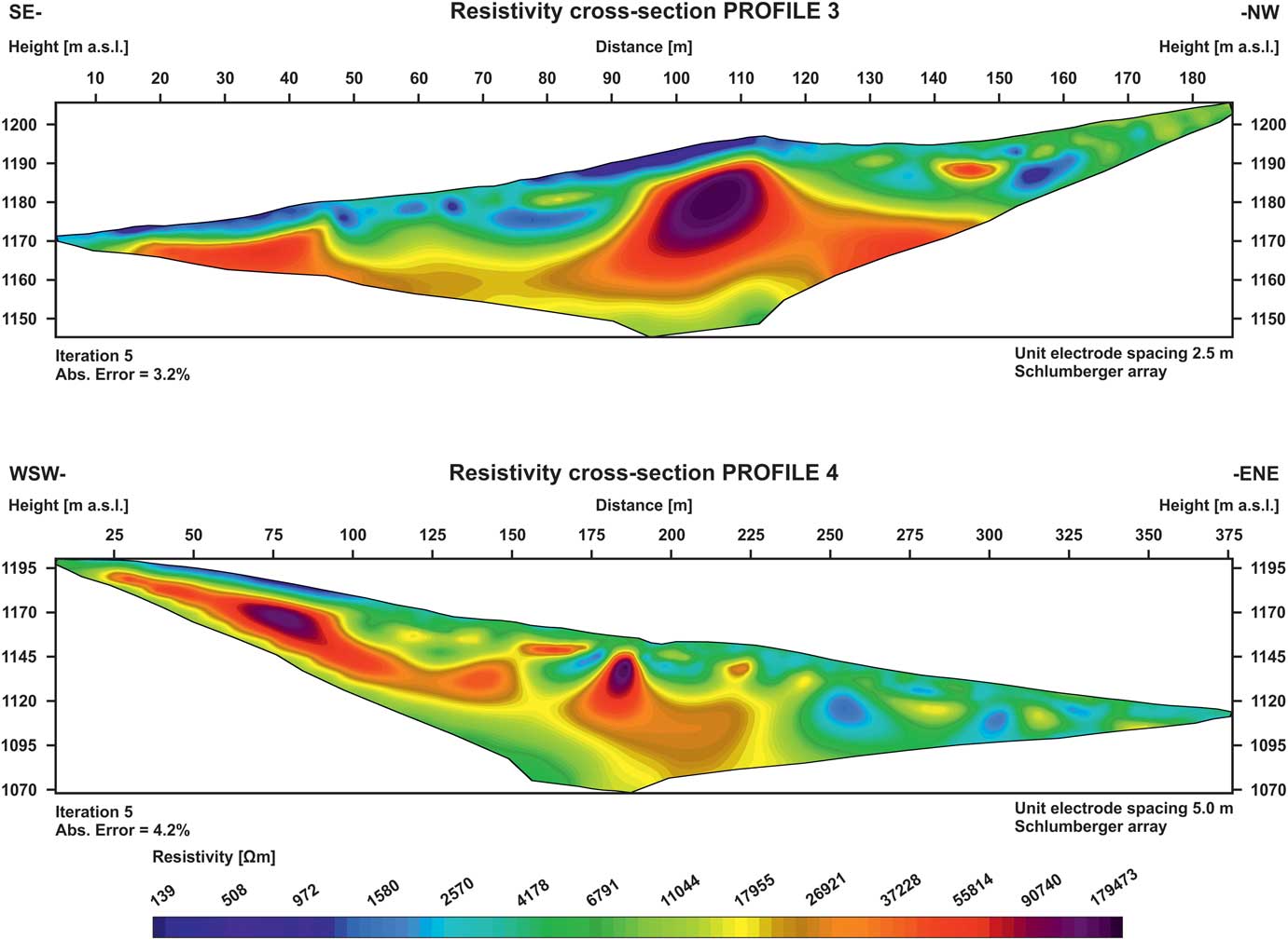
The data obtained using ERT imaging varied significantly depending on the electrode spacing used and the length of the profile. Profile 3 (see Fig. 2b for location) ran parallel to the glacier front; for this reason, we used an electrode spacing of 2.5 m. In this profile, we covered a distance of 200 m and a much higher depth range was achieved, i.e., up to 40 m (Fig. 10) compared to the previous ERT profiles.
(color online) ERT Profile 3, 200 m long, located on the frontal glacier moraine. It presents a high-resistivity anomaly identified as a dead-ice core. Perpendicular to Profile 3 is the ERT Profile 4. This is a 400-m-long profile located on the frontal glacier moraine and forefield; it shows an upper and deeper permafrost layer.

This ERT profile cuts Profile 1 almost at a right angle after 160 m. The near-surface layer is highly variable, although dominated by a low resistive anomaly approximately half way up the profile. This anomaly is found in a sparsely vegetated moraine hill with a stable surface, where fine-grained till has not been washed out. The resistivity in this area barely reaches ca. 0.5 kΩm, as a consequence of the presence of fine-grained wet material. Higher retention inside this layer may be also the cause of a huge, highly resistive anomaly directly below it. This structure is most likely an ice core of glacial origin, as previously described by Østrem (Reference Østrem1964), which would appear in the ERT image as a characteristic zone showing large differences in resistivity values between these layers. A fine-grained upper layer also saturated with water is visible in the initial lower section of the profile, in close proximity to the glacier, where the terrain is also highly saturated with water from an ablation outflow. The resistivity values in this zone reach only 0.5–2 kΩm. This anomaly is also near a highly resistive layer directly underneath. This upper layer is 2–3 m deep, while the highly resistive layer is found deeper down the profile, between 50 and 80 m and 125 and 200 m. The resistivity values in the upper layer are slightly higher, reaching 4 kΩm. Drainage in this section is more efficient than in the surroundings, and the ground was also drier. However, the most interesting feature here was a highly resistive 40-m-thick anomaly arranged as an uneven layer starting at a depth of ca. 5–17 m. The resistivity values for this layer range from 25 kΩm to over 100 kΩm. This is most likely a permafrost layer with an ice core, as described above, remaining from the glacier after retreat (Østrem, Reference Østrem1964).
Profile 4 was perpendicular to Profile 3 and covered a length of 400 m with an electrode spacing of 5 m (Fig. 10). Here, we aimed to identify the level of spatial variability of the active permafrost in depth and its maximum depth. A highly resistive layer, starting at values of 11 kΩm and reaching up to 40–100 kΩm, is already apparent near the glacial front below the active layer, in a zone where resistivity values otherwise range from 0.9 to 4 kΩm. The ERT results shown in Profile 4 perfectly fit the results obtained for Profile 3, thus confirming the occurrence of an ice core, ca. 30 m thick approximately ca. 110 m up the profile. However, the extent of the frozen material may reach significantly lower depths. The high resistive anomaly starts to stratify ca. 120 m up the profile. In addition, a highly resistive discontinuous anomaly appears visible at a relatively shallow level below the active layer, analogous to the high-resistive layer found higher up below the unfrozen sediments and visible in Profiles 1 and 2. Below, there is also a layer of decreased resistivity followed by another high resistive anomaly section. This stratification may indicate the presence of two layers of permafrost, where the second one can penetrate also the bedrock.
DISCUSSION
These results provide two tiers of information: (1) information on the material variability within the glacier, i.e., the structure of the ice and its interaction with the slope/moraine material, and (2) geophysical information involving the presence and characteristics of boundaries between temperate and cold ice zones within the glacier and similar geophysical characteristics in the forefield permafrost. In both cases, the results can be identified as describing a glacial–periglacial system.
Material aspects of the glacial–periglacial complex
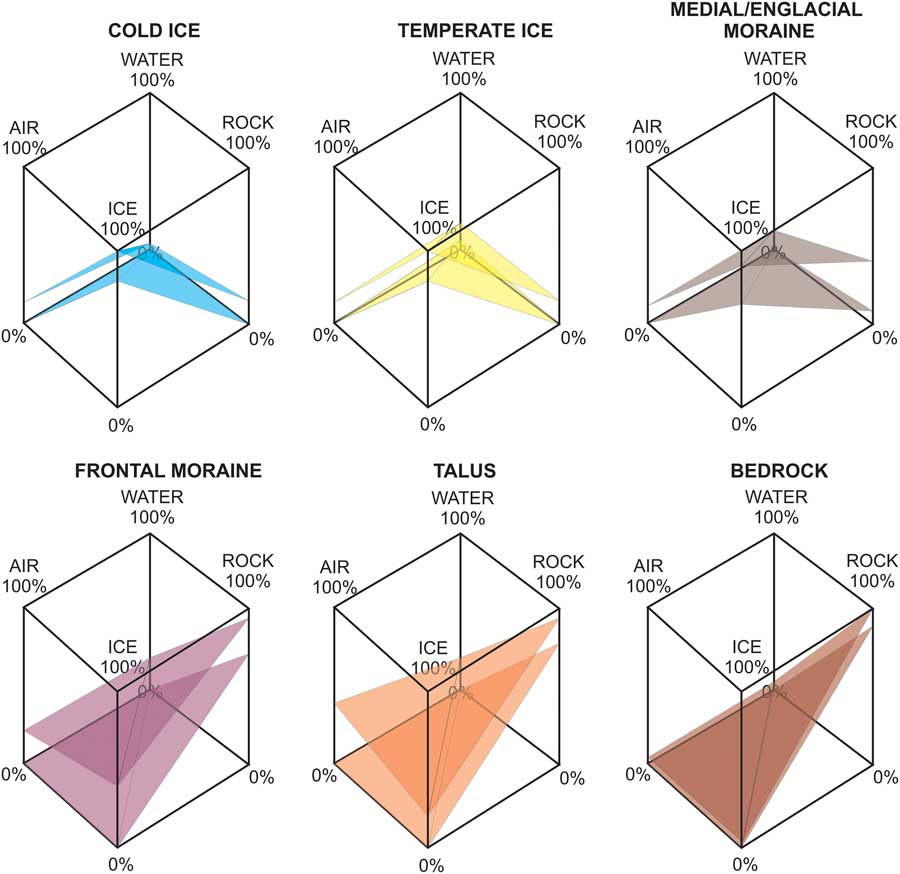
Our results show glacial–periglacial relationship as a series of structures arranged as a coherent system. The individual elements of the system can be generally identified as mineral, ice, liquid water, or air, which associate to form the distinct structures contained within the whole system. Figure 11 shows a schematic illustration of some selected elements of the glacial- periglacial complex defined from these four basic components.
(color online) Composition of selected forms from the glacial and periglacial environments based on their four main components: ice, air, water, and rock. The upper and lower surfaces represent the maximum and minimum contents of the components forming the structure. The larger the range between surfaces, the highest the potential variability in composition is. Homogeneous forms only present one dominating component. Some structures share the proportional composition of these four elements. Thus, boundaries between different structures sharing proportional composition are frequently difficult to resolve.

The GPR survey, as summarized in Figures 5–8, field observations, and the data analysis showed how each these elements can associate very broadly. Thus, the overall system appears as a mix complex where boundaries are not always clearly obvious but rather appear as transitional zones, preventing identification of individual structures. Clear-cut boundaries are mainly obvious between homogeneous media, often coming as a mixture of different materials. By identifying the different material components of this complex, we can also distinguish difference facies characteristic of different geological formations and consisting mostly of ice and sediments. Ice often acts as a binding agent due to its visco-plastic properties; however, the presence of ice mixed with sediments is precisely what allows us to study the glacial–periglacial system as one complex.
Occasionally, it was difficult to determine the location of the boundary between the glacier and its base, particularly in areas where mineral material, glacial ice, and snow mixed together. This was evident in the northern part of the glacier, where the GPR Stor 2 profile was identified as an internal moraine mixed with the glacier slope material (Fig. 6). The amount of sediment increases nearer the slope, increasing facial diversity with ice predominantly present in the farther sections, and sediment materials gradually increase towards the slope, finally ending in a rock surface covered with clastic material. The glacier dynamic will evolve in the same direction. Identifying the glacier boundary (glacial ice) in such settings poses many difficulties and may be subjective. Radar profiles, however, show the distribution of ice and sediment (moraine) material quite accurately, allowing much higher precision to determine the relationship between glacial ice and slope sediments, compared to surface observations or analyses of aerial photographs (Bernard et al., Reference Bernard, Friedt, Saintenoy, Tolle, Griselin and Marlin2014).
The variability resulting from mixing multi-fraction sedimentary material with glacial ice is high, and it tends to relate to gravitational processes of sediment transport along the slope and its subsequent incorporation into the glacier, along with snow sedimentation and further transport based on plastic deformation of ice and its creeping. The mixture of sediments and ice visible in the near-surface part of the radar profiles (Figs. 5–7) as debris bands and internal moraine forms the “cold” part of the glacier in glaciological terms, and the zone “encompassed by permafrost” as defined based on permafrost science. In many places, the transition from the periglacial to the glacial material was smooth and therefore a clear differentiation is impossible. Indeed, in this case the periglacial processes gradually replace the glacial ones, as previously described (Seppi et al., Reference Seppi, Zanoner, Carton, Bondesan, Francese, Carturan, Zumiani, Giorgi and Nifo2015).
Glacial till is a material frequently involved in a series of complex processes (e.g., Boulton and Hindmarsh, Reference Boulton and Hindmarsh1987; Alley, Reference Alley1989; Knight, Reference Knight1989, Piotrowski, Reference Piotrowski, Mickelson, Tulaczyk, Krzyszkowski and Junge2001; Waller, Reference Waller2001; van der Meer et al., Reference van der Meer, Menzies and Rose2003). To this end, Knight (Reference Knight1997) described the number of processes linked to accretion of ice, ice diagenesis, entrainment of debris, and thickening of sequence as a review in basal ice formation mechanisms. However, not all of these processes are genetically related to glacial ice. A detailed description of debris entrainment in Storglaciären and its polythermal structure can be found in Jansson et al. (Reference Jansson, Nälsund, Petterson, Richardson-Nälsund and Holmlund2000). According to Knight, it is also possible for regelation or congelation ice to be formed under the glacier. These types of ice are included into the glacier, together with sediments, and can be differentiated from the ice formed in the glacial accumulation zone based on e.g., isotopic tests or studies of the ice/gas composition (Knight, Reference Knight1997). Regelation, or even congelation, of ice can be accumulated beyond the glacial base as a consequence of stress changes and related melt or freeze in given conditions. It occurs to a much greater extent in the accumulation area of glaciers as internal accumulation. This type of ice accumulation can represent anything between 5 and 70% of all the glacial accumulation (Trabant and Mayo, Reference Trabant and Mayo1985; Bazhev, Reference Bazhev1997; Rabus and Echelmeyer, Reference Rabus and Echelmeyer1998). In Storglaciären, internal accumulation is responsible for ca. 3–5% of the annual accumulation for the entire glacier (Schneider and Jansson, Reference Schneider and Jansson2004). This type of ice is technically periglacial in genetic terms, as the glacier itself cannot create it. In the genetic sense, only the glacial body of ice can be considered glacier ice, which forms during the accumulation and metamorphism of snow. Thus, the glacial environment involves also the presence of genetically different types of ice, including those typical for the periglacial environment. Frost penetration, however, is a static process and the movement of the glacier does not limit it significantly. On the other hand, glacier dynamic can be modified by frost penetration to a significant extent.
Following the traditional definition as non-frozen partly water filled ground, the active permafrost layer starts under the marginal protruding section of the glacial tongue. Its thickness increases in the forefield; however, the forefield permafrost experiences aggradation for retreating glaciers, particularly due to mean annual air temperature, an area whose temperature is over –4°C. This section is apparent in the ERT 1 profile in the form of a high-resistance layer under a superficially dried and subsequently flooded active layer (Fig. 9). Data from the Profiles 3 and 4 (Fig. 10) allows preliminarily concluding that the maximum thickness of the glacier permafrost layer, identified here as a dead-ice core, reaches ca. 40–50 m under the ground surface.
Geophysical characteristics of the glacial-periglacial complex
The geophysical characteristics of the glacial–periglacial complex can be described based on the glacier thermal characteristics. Storglaciären is classified as a polythermal glacier, a characteristic that is apparent from the radar surveys, which clearly show the presence of both cold and temperate ice layers within the glacier. The cold upper layer of ice in a polythermal glacier is analogous to the permafrost found in the periglacial environment, as it is the result of the energy balance at the glacier surface and the advection of temperate ice through the glacier flow (Hooke et al., Reference Hooke, LeB., Gould and Brzozowski1983; Blatter and Hutter, Reference Blatter and Hutter1991; Krass, Reference Krass1991; Petterson et al., 2003). This implies that the cold surface layer is sensitive to climatic variations directly, through changes in energy balance and heat transfer at the glacier surface, and indirectly, through feedback processes led by variations in glacier flow caused by changes in mass balance (Petterson et al., 2003); both processes are geophysical in nature (Petterson et al., 2007). Cold ice layer formed this way can be identified as glacial permafrost, differing from the periglacial permafrost by the lack of an active layer (in the periglacial sense of the term), which following phase transition into a liquid form flows down the glacier as ablation water (Dobiński, Reference Dobiński2011a).
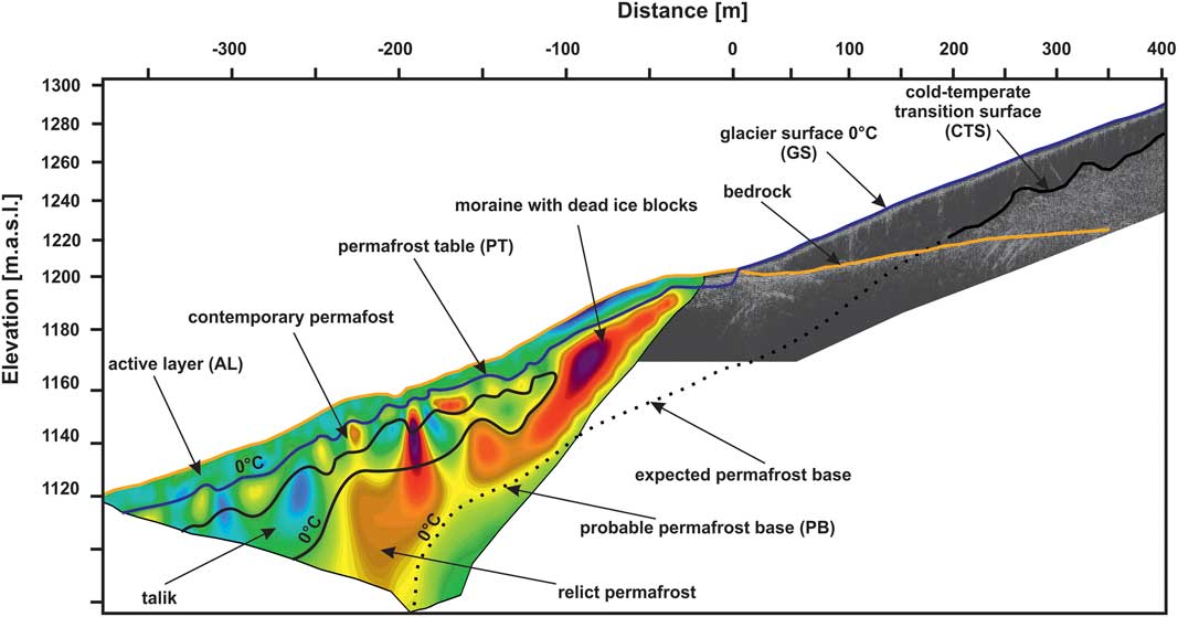
The thickness of the cold surface layer is a function of the surface energy flux, the net ablation at the glacier surface, the liquid-water content of the ice entering the cold surface layer, and the movement of the glacier. A negative temperature gradient through the cold surface layer causes the base of the cold layer to migrate downwards as the containing water temperate ice freezes further (Petterson et al., 2007). This process is also analogous to permafrost formation in periglacial environments. Downwards migration of CTS is as it deepest in the frontal part of the glacier (Pattersson, 2002). At a certain point, CTS penetrates below the bottom of the glacier causing its front to freeze to the ground as a consequence of climatic factors. This is the place where CTS enters the surface of the PB of the traditional permafrost layer, as the zone where the temperature is usually close to 0°C (the CTS-PB complex is marked in Figs. 1 and 12). This is also the specific place where the glacier’s properties change, for example, as a decrease in its erosional force.
(color online) Geophysical model of the glacier–permafrost interaction. The figure shows the location of the active layer within the glacier (glacier surface) and the periglacial environment (ca. 2–5 m depth). The second surface represents the cold-temperate transition surface (CTS), located at the bottom of the cold-ice layer and continuing as a permafrost base (PB), the lower border of the permafrost layer. Both surfaces, drawn from empirical data, show a geophysical continuum between the glacial and periglacial environments, as defined by Dobiński (Reference Dobiński2006; after Dobiński and Glazer, [Reference Dobiński and Glazer2016] with modifications).

The occurrence of this CTS-PB surface is not limited to the space under the glacier. It reaches further than the front of the glacier fully transitioning into the permafrost present in the glacier forefield. Obviously, a continuation of the CTS-PB complex is possible only under climatic conditions in the glacial forefield that allow for the formation of permafrost, i.e., –1°C MAAT. This condition is met in the case of Storglaciären and its forefield. Previously published data shows that the cold ice layer on Storglaciären reaches up to approximately half of the glacial tongue. Similar work also included detailed CTS data on the glacier’s evolution for the period 1989–2009, and, in particular, on its dependence on snow (Pettersson et al., 2003; Gusmeroli et al., Reference Gusmeroli, Jansson, Petterson and Murray2012). This glacier is therefore frozen at its front, as shown by GPR and ERT studies, and potentially to the surrounding slopes, up to a depth of ca. 25–40 m in its northern slope and to 15–30 m in its southern slope. At these depths, the CTS of the glacier may even penetrate further in the slope configured as the PB of the periglacial permafrost.
The frost penetration process, although significantly altering the thermal structure of the glacier and having an impact on a number of its properties, such as water content, movement speed, and method, is not a pure glacial process, as it is also influenced by climate. Frost penetration of the “icy-lithosphere” as defined by Shumskii (Reference Shumskii1964) occurs both within the glacier and outside it. The shift of the CTS towards the surface or deeper inside the glacier is linked to climate variations, i.e., temperature, on the glacier surface. This is further shown by the strong correlation (R2=0.87) found between the thickness of the cold ice layer in Storglaciären and the BTS temperature. A 1°C increase in BTS will lead to a change in the upper boundary conditions of the cold surface layer, thinning somewhere between 3 and 12 m (Pettersson et al., Reference Pettersson, Jansson, Huwald and Blatter2007). The BTS method was developed to detect permafrost at low depths in periglacial environment (Haeberli, Reference Haeberli1973, Reference Haeberli1985). Moreover, the temperature of the cold ice changes seasonally. Given said that, a zone of zero annual amplitude of seasonal temperature changes (ZAA) can be found both in cold ice and permafrost (cf. fig. 5 in Pettersson et al., Reference Pettersson, Jansson, Huwald and Blatter2007).
Glacier–permafrost association model
Set against our results, the association between the glacier and the permafrost should be described in geophysical terms, particularly as they share common frost penetration properties. Both the glacier and the forefield present two distinct summer surfaces, an upper and a lower surface, remaining at temperature close to or equal to 0°C. The layer with negative temperature, which is located between those surfaces, continues from the glacial onto the periglacial environment, connecting them in the geophysical sense. The first upper surface is simply the glacier surface (GS). Underneath, there is a layer of frozen cold ice (Fig. 12). In the glacier forefield, the analogous surface continues into the bottom of the active layer as permafrost table (PT) within moraine deposits. The lower surface is found between the temperate and cold ice in the polythermal glacier environment, and it is known as the CTS, where the temperature is usually lower than 0oC and is determined by the pressure melting point (PMP). Its counterpart in the glacial forefield is the PB, the lower boundary of the permafrost layer (Figs. 1 and 12). The CTS-PB surface is thus continuous, forming an axis with similar thermal properties albeit occurring in different media. From the geophysical sense, this CTS-PB surface integrates both the glacial and the periglacial environments (Dobiński et al., Reference Dobiński2006, Reference Dobiński2011b; Dobiński 2011) similarly as GS-PT surface above, as shown in Figures 1 and 12.
The physical characteristics of the thermal structure of glaciers allow utilising models derived from permafrost studies (Dobiński, Reference Dobiński2006, Reference Dobiński2011a, Reference Dobiński2011b, Reference Dobiński2012). Our results here validate the glacial use of such models, previously hypothesised as possible.
CONCLUSIONS
Long-term frost penetration in the Storglaciären area involves both the upper layer of the glacier and the upper ground layer of the forefield. As a result, the cold glacial ice layer is formed in glacial environment, and permafrost layer on the forefield. Both layers are the result of the same climate impact in the Tarfala area. Cold ice thickness and variability are shown in the GPR results. The ERT results, on the other hand, are useful to identify the variability of the permafrost along the glacier forefield and the presence of dead ice blocks.
In the upper accumulation area of the glacier, in its lateral margins, the GPR survey shows not always a clear glacier boundary. These results reflect how intensive accumulation of slope sediments on the glacier surface can be gradually incorporated into the glacial ice, changing the characteristics of the GPR image. This process also illustrates how the glacial and periglacial environments overlap in the accumulation area of the glacier, which at the same time is strongly linked to permafrost penetration. As a result of this process, the transition between the glacial and the periglacial environment is gradual with unclear discontinuous or transitional boundaries.
The GPR survey also shows a glacier front frozen to its bed, along with the till material it carries, suggesting a continuous ground temperature below 0oC. Ground permafrost aggradation starts under the glacier. To this end, the layer of permafrost present in the glacial forefield is visible in the ERT images immediately before the glacier front. This frozen soil, however, is significantly disturbed with ablation water percolation from the glacier. Nevertheless, our results confirm and the conducted research confirms the hypothesis and proposed theory regarding the geophysical (thermal) relation between the glacial permafrost and the periglacial permafrost on the forefield.
The boundary separating the cold and temperate ice (CTS) forms an environmental continuum with its equivalent boundary in the periglacial environment, the PB. This CTS-PB surface is a specific environmental axis around which the glacial and periglacial environments evolve. A similar seasonal axis, binding the glacial and the periglacial environment, is the boundary formed by the glacier surface and the permafrost table (GS-PT). This boundary is directly influenced by seasonal climatic variations.
Accreted ice, congelation ice, regelation ice and the ice types linked to internal accumulation are non-glacial ice in the genetic sense, as they cannot build to initiate a glacier. A similar case is found in the periglacial zone, where the dead ice of glacial origin found in the moraine belongs to the periglacial environment. Thus, both in the geophysical and purely material terms, the glacial and periglacial environments do penetrate each other.
Acknowledgments
This article is one of the results of a research project funded by the National Science Centre, Poland (NCN) DEC-2012/07/B/ST10/04268. The publication has been (partially: English edition) financed from the funds of the Leading National Research Centre (KNOW) received by the Centre for Polar Studies of the University of Silesia, Poland. Dr. Peter Jansson from Department of Physical Geography, Stockholm University is acknowledged for his help in manuscript preparation. Data supplied by Tarfala Research Station is gratefully acknowledged. The careful reviews by two anonymous reviewers significantly helped us improve the paper. We are most grateful to Dr. Derek Booth, Senior Editor, and Associate Editor Dr. James Shulmeister, who provided additional suggestions, helping us to improve the paper further. AMDG.