2.1 Physical system

A sketch of the physical configuration is presented in figure 1. A circular cylinder of diameter $D$ is immersed in linear planar shear flow. The body axis is aligned with the $z$ axis. The problem is studied in two dimensions, in the $(x,y)$ plane, and the oncoming flow is parallel to the $x$ axis. The coordinates $x$ and $y$ are non-dimensionalized by $D$ . The dimensional oncoming flow velocity is given by $\boldsymbol{U}^{\infty }=\{u^{\infty },0\}^{\text{T}}=\{u_{0}(1+\unicode[STIX]{x1D6FD}y),0\}^{\text{T}}$ , where $u_{0}$ is the free-stream velocity at the centre of the cylinder and $\unicode[STIX]{x1D6FD}$ is the non-dimensional shear parameter, $\unicode[STIX]{x1D6FD}=(\text{d}u^{\infty }/\text{d}y)/u_{0}$ . The Reynolds number based on $u_{0}$ and $D$ , $Re~=\unicode[STIX]{x1D70C}_{f}u_{0}D/\unicode[STIX]{x1D707}$ , where $\unicode[STIX]{x1D70C}_{f}$ and $\unicode[STIX]{x1D707}$ are the fluid density and dynamic viscosity, is set to $100$ . The two-dimensional incompressible Navier–Stokes equations are employed to predict the flow dynamics.

Figure 1.

Sketch of the physical configuration.

In the elastically mounted body case, the cylinder is free to oscillate in the in-line ( $x$ axis) and cross-flow ( $y$ axis) directions. The origin of the $(x,y)$ frame coincides with the position of the body axis when the oscillator is at rest in quiescent fluid. The oscillator is characterized by the body mass per unit length $\unicode[STIX]{x1D70C}_{c}$ and the structural stiffnesses and damping ratios in both directions, $k_{i}$ and $\unicode[STIX]{x1D709}_{i}$ , where the subscript $i$ designates the $x$ or $y$ direction. All the physical quantities are non-dimensionalized by $D$ , $u_{0}$ and $\unicode[STIX]{x1D70C}_{f}$ . The non-dimensional mass is defined as $m=\unicode[STIX]{x1D70C}_{c}/\unicode[STIX]{x1D70C}_{f}D^{2}$ ; it is set to $2$ . The non-dimensional cylinder displacement, velocity and acceleration in the $i$ direction are denoted by $\unicode[STIX]{x1D701}_{i}$ , $\dot{\unicode[STIX]{x1D701}_{i}}$ and $\ddot{\unicode[STIX]{x1D701}_{i}}$ . The force coefficient in the $i$ direction is defined as $C_{i}=2F_{i}/\unicode[STIX]{x1D70C}_{f}Du_{0}^{2}$ , where $F_{i}$ denotes the sectional fluid force in the $i$ direction. The body dynamics in the $i$ direction is governed by a forced, second-order oscillator equation:

The reduced velocity in the $i$ direction is defined as $U_{i}^{\ast }=1/f_{nat,i}$ , where $f_{nat,i}$ is the non-dimensional natural frequency in vacuum, $f_{nat,i}=D/2\unicode[STIX]{x03C0}u_{0}\sqrt{k_{i}/\unicode[STIX]{x1D70C}_{c}}$ . In the following, the structural stiffnesses are the same in both directions and the reduced velocity and natural frequency of the oscillator are referred to as $U^{\ast }=U_{x}^{\ast }=U_{y}^{\ast }$ and $f_{nat}=f_{nat,x}=f_{nat,y}$ . The damping ratio is set equal to zero in both directions to allow maximum amplitude oscillations ( $\unicode[STIX]{x1D709}_{i}=0$ ).

The behaviour of the flow–structure system is explored in the ( $\unicode[STIX]{x1D6FD}$ , $U^{\ast }$ ) parameter space. The shear parameter ranges from $0$ to $0.4$ and the reduced velocity from $2$ to $14$ . The same range of $\unicode[STIX]{x1D6FD}$ is considered in the fixed body case.

Figure 2.

Schematic view of the mapping approach.

2.2 Numerical method

A general mapping approach for moving bodies in non-uniform flow, that avoids domain deformation and keeps uniform free-stream conditions is introduced. The mapping is decomposed in three steps, as depicted in figure 2. At step 1, the system is described in the laboratory frame $(x,y)$ . The cylinder axis is located at $\{\unicode[STIX]{x1D701}_{x},\unicode[STIX]{x1D701}_{y}\}_{(x,y)}^{\text{T}}$ and is moving with velocity $\{\dot{\unicode[STIX]{x1D701}_{x}},\dot{\unicode[STIX]{x1D701}_{y}}\}_{(x,y)}^{\text{T}}$ . The $(x_{c},y_{c})$ frame, attached to the body axis and in translation with respect to the $(x,y)$ frame, is indicated in the sketch. The flow is governed by the two-dimensional incompressible Navier–Stokes equations,

where $t$ is the non-dimensional time and $\boldsymbol{V}$ and $P$ denote the non-dimensional velocity and pressure fields. Far from the body, the non-dimensional free-stream velocity $\boldsymbol{V}^{\infty }$ is given by the shear flow condition. A no-slip condition is imposed at the body surface; therefore, the non-dimensional velocity of the fluid at the surface, $\boldsymbol{V}^{\boldsymbol{b}}$ , is equal to the body velocity. A change of the flow variables is considered at step 2. The new velocity field $\boldsymbol{V}_{\boldsymbol{u}}$ is associated with a uniform far-field condition $\boldsymbol{V}_{\boldsymbol{u}}^{\infty }$ and a non-uniform condition at the body surface $\boldsymbol{V}_{\boldsymbol{u}}^{\boldsymbol{b}}$ . At step 3, the system is described in the body frame $(x_{c},y_{c})$ . This frame change is accompanied by a new change of the flow variables. In the resulting formulation, the system is seen as a stationary cylinder immersed in a uniform but time-dependent flow. A new set of boundary conditions, $\boldsymbol{V}_{\boldsymbol{c}}^{\infty }$ and $\boldsymbol{V}_{\boldsymbol{c}}^{\boldsymbol{b}}$ , is obtained.

The time and space derivatives in the laboratory and body frames verify

The transformed Navier–Stokes equations, obtained by substituting variables $x$ , $y$ , $t$ , $\boldsymbol{V}$ and $P$ by $x_{c}$ , $y_{c}$ , $t_{c}$ , $\boldsymbol{V}_{\boldsymbol{c}}$ and $P_{c}$ in the flow equations (2.2), can be expressed as follows: The source term $\boldsymbol{S}$ takes into account the frame motion and the shear of the oncoming flow. The $x$ and $y$ components of $\boldsymbol{S}$ are given by where $V_{cx}$ and $V_{cy}$ are the $x$ and $y$ components of $\boldsymbol{V}_{\boldsymbol{c}}$ . In the fixed body case, the same formulation is employed, with $\unicode[STIX]{x1D701}_{i}=\dot{\unicode[STIX]{x1D701}_{i}}=\ddot{\unicode[STIX]{x1D701}_{i}}=0$ .

Equations (2.4) are solved numerically. The computations are performed with the finite-volume code Numeca Fine/Open (www.numeca.com) which employs a preconditioned multigrid method (Liu, Zheng & Sung Reference Liu, Zheng and Sung1998). Viscous and inviscid fluxes, as well as the source term $\boldsymbol{S}$ are computed via second-order schemes. A second-order time integration is performed using a dual-time stepping method with a Runge–Kutta scheme. At each time step, the structural dynamics equations (2.1) are solved implicitly following the same pseudo-time integration scheme as for the fluid equations.

The flow is discretized on a non-structured grid in a rectangular computational domain. The cylinder is located at $(x_{c},y_{c})=(0,0)$ . The domain extends from $x_{c}=-L_{x}/2$ to $x_{c}=L_{x}/2$ in the in-line direction and from $y_{c}=-L_{y}/2$ to $y_{c}=L_{y}/2$ in the cross-flow direction. An unsteady far-field condition based on the Riemann invariants is used at the external boundaries of the domain and is updated at each inner iteration, according to the velocity of the frame attached to the body. A non-uniform Dirichlet condition is used at the body surface. All the computations are initialized with a fixed body immersed in uniform flow.

A convergence study has been carried out in the fixed and elastically mounted body cases in order to set the numerical parameters. As an important effect of the blockage ratio was reported in the literature (Kang Reference Kang2006), particular attention was paid to the size of the computational domain. Some convergence results obtained in the elastically mounted body case have been selected and are presented in table 1. The root-mean-square (r.m.s.) values of the body displacement fluctuations and the dominant cross-flow oscillation frequencies $f_{y}$ , obtained for three sets of numerical parameters, are compared for $(\unicode[STIX]{x1D6FD},U^{\ast })=(0.15,6)$ and $(\unicode[STIX]{x1D6FD},U^{\ast })=(0.4,6)$ , i.e. for an intermediate value of the shear parameter and for the largest value studied in this work, at a reduced velocity where the cylinder exhibits large-amplitude vibrations, as shown in § 4.1. In this table and in the following, the symbol $^{\prime }$ designates the r.m.s. value of the variable fluctuation about its time-averaged value. Three grids are considered. All grids present the same resolution and only differ by the size of the computational domain. The grid resolution has been the object of a separate convergence study. Different time steps $\unicode[STIX]{x0394}t$ and numbers of inner iterations $n_{i}$ are considered in this table. For $\unicode[STIX]{x1D6FD}=0.15$ , significant discrepancies are noted between cases 1 and 2, while the results obtained in cases 2 and 3 are comparable. For $\unicode[STIX]{x1D6FD}=0.4$ , the responses show very low sensitivity to the numerical parameters, and the results obtained in the three cases are similar. The proximity of the responses in cases 2 and 3, for $\unicode[STIX]{x1D6FD}=0.15$ and $\unicode[STIX]{x1D6FD}=0.4$ , illustrates the convergence of the results with respect to the numerical parameters. The numerical parameters of case 2 were selected in this study. The corresponding grid is composed of $65\times 10^{3}$ cells. Complementary results on blockage effect and validation of the present simulation approach in the uniform flow case are presented in appendices A and B.

Table 1.

Influence of the domain size, time step and number of inner iterations on the body responses, for $U^{\ast }=6$ .

The analyses reported in this paper are based on time series of more than $50$ cycles of the system, collected after convergence of the time-averaged and r.m.s. values of the fluid force coefficients.

3.1 Fluid forces

The time-averaged fluid force coefficients are plotted as functions of $\unicode[STIX]{x1D6FD}$ in figure 3(a). In this plot and in the following, $\overline{\phantom{a}}$ designates the time-averaged value. In the in-line direction, the time-averaged force globally decreases as the shear parameter is increased. Three branches can be identified. In the first branch ( $\unicode[STIX]{x1D6FD}\in [0,0.2]$ ), $\overline{C_{x}}$ slowly decreases as a function of $\unicode[STIX]{x1D6FD}$ . A similar trend was observed by Lei et al. (Reference Lei, Cheng and Kavanagh2000), Kang (Reference Kang2006) and Cao et al. (Reference Cao, Ozono, Tamura, Ge and Kikugawa2010) in the same range of $\unicode[STIX]{x1D6FD}$ , at comparable Reynolds numbers. As the shear parameter is increased above $0.2$ , $\overline{C_{x}}$ reaches the second branch ( $\unicode[STIX]{x1D6FD}\in [0.2,0.3]$ ), with substantially lower values than in the first branch. In this second branch, $\overline{C_{x}}$ remains close to constant as a function of $\unicode[STIX]{x1D6FD}$ . $\overline{C_{x}}$ is also constant in the third branch, which corresponds to the range $\unicode[STIX]{x1D6FD}\in [0.3,0.4]$ . A negative time-averaged force is noted in the cross-flow direction. The three branches are less clearly defined but still visible in the evolution of $\overline{C_{y}}$ . In the first branch, $\overline{C_{y}}$ linearly decreases as a function of $\unicode[STIX]{x1D6FD}$ ; this evolution is consistent with the data reported in previous works. At higher shear (second and third branches), $\overline{C_{y}}$ is close to constant. The r.m.s. values of the force coefficient fluctuations are plotted in figure 3(b). In the first branch, the force fluctuations tend to increase with the shear. Distinct trends are noted during the transition between the first and second branches: $C_{y}^{\prime }$ abruptly drops while $C_{x}^{\prime }$ slightly increases. In the second branch, the force fluctuations increase as functions of $\unicode[STIX]{x1D6FD}$ in both directions. Residual oscillations can be noted up to $\unicode[STIX]{x1D6FD}=0.33$ approximately, but the force fluctuations tend to vanish in the third branch.

Figure 3.

Fluid force statistics in the fixed body case: (a) time-averaged values of the fluid force coefficients and (b) r.m.s. values of the fluid force coefficient fluctuations as functions of $\unicode[STIX]{x1D6FD}$ , in both directions. Coloured symbols in (a) represent the values of $\overline{C_{x}}$ obtained in the elastically mounted body case, in selected points of the ( $\unicode[STIX]{x1D6FD}$ , $U^{\ast }$ ) parameter space indicated in figure 8(c).

The first two branches identified in figure 3 are called branches L and H, in reference to the low and high values of $\unicode[STIX]{x1D6FD}$ . The third branch, where the constant fluid forcing suggests a steady flow behaviour, is called branch S. The branches are indicated in figure 3(a).

Figure 4.

Fluid force spectral content in the fixed body case: power spectral density of the fluid force coefficient as a function of $\unicode[STIX]{x1D6FD}$ , in the (a) in-line and (b) cross-flow directions. For each $\unicode[STIX]{x1D6FD}$ , the power spectral density is normalized by the magnitude of its largest peak. The colour levels range from $0$ (white) to $1$ (black). Coloured symbols in (a) represent the dominant frequency of the in-line force obtained in the elastically mounted body case, in selected points of the ( $\unicode[STIX]{x1D6FD}$ , $U^{\ast }$ ) parameter space indicated in figure 8(c).

The spectral contents of the fluctuating fluid forces are examined in figure 4, which represents, for each direction, the power spectral density (PSD) of the force coefficient as a function of $\unicode[STIX]{x1D6FD}$ . Unless otherwise stated, the spectral analyses reported in this paper are based on the Fourier transform of the entire time series collected after convergence. When the oncoming flow is uniform ( $\unicode[STIX]{x1D6FD}=0$ ), the fluid forces are dominated by a single frequency (i.e. sinusoidal) and the in-line force fluctuations occur at twice the cross-flow force frequency, as expected due to the cross-flow symmetry of the configuration. For $\unicode[STIX]{x1D6FD}>0$ , the symmetry is broken and a spectral component emerges, at the cross-flow force frequency, in the spectrum of $C_{x}$ ; the relative contribution of this new component increases as a function of $\unicode[STIX]{x1D6FD}$ and it becomes predominant close to $\unicode[STIX]{x1D6FD}=0.1$ .

The three branches identified above on the basis of the force statistics are associated with distinct frequency contents. The force frequencies slightly decrease as functions of $\unicode[STIX]{x1D6FD}$ on branch L. After a non-monotonic behaviour around $\unicode[STIX]{x1D6FD}=0.2$ , they reach a plateau in the H-branch region, where they are found to be much lower than in the L-branch region. On branch H, other harmonics appear in the force spectra. In the cross-flow direction, their amplitudes are limited and $C_{y}$ remains close to harmonic. The relative contribution of each harmonic to $C_{x}$ spectrum varies as a function of $\unicode[STIX]{x1D6FD}$ and the resulting signal is generally not harmonic. For $\unicode[STIX]{x1D6FD}>0.3$ , in the S-branch region, the force fluctuations tend to disappear and the PSD are not computed.

The data reported in figures 3 and 4 reveal non-monotonic evolutions of the fluid forces in the region of transition between branches L and H. In this region, the flow solution appears to switch from one branch to the other. This behaviour may indicate an overlap of branches L and H. It is recalled that, in the present work, all the simulations are initialized with a fixed cylinder immersed in uniform flow. Additional simulations with different initial conditions have shown that hysteresis effects may be encountered in the L–H transition region.

The analysis of the fluid forces suggests that the flow undergoes three successive regimes within the range of $\unicode[STIX]{x1D6FD}$ under study. These regimes are investigated in the following.

3.2 Flow regimes

Figure 5.

Analysis of the three flow regimes identified in the fixed body case: (a) schematic view of the cross-flow force dominant frequency as a function of $\unicode[STIX]{x1D6FD}$ ; (b,c,d) selected time series of the cross-flow force coefficient (solid) and spanwise vorticity at $(x,y)=(10,0)$ (dashed), and instantaneous iso-contours of the spanwise vorticity ( $\unicode[STIX]{x1D714}_{z}\in [-\unicode[STIX]{x1D6FD}-1,-\unicode[STIX]{x1D6FD}+1]$ ) in the vicinity of the body at selected instants (indicated by vertical dashed lines in the time series), for (b) $\unicode[STIX]{x1D6FD}=0.1$ , (c) $\unicode[STIX]{x1D6FD}=0.25$ and (d) $\unicode[STIX]{x1D6FD}=0.4$ . The black triangle in the snapshots indicates the monitor point where the vorticity is sampled.

A schematic view of the evolution of the cross-flow force dominant frequency ( $f_{C_{y}}$ ) as a function of $\unicode[STIX]{x1D6FD}$ is presented in figure 5(a). The three regions of the parameter space associated with the branches identified in § 3.1 (L, H and S) are indicated in this plot. A typical value of $\unicode[STIX]{x1D6FD}$ is selected in each region in order to describe the main properties of the corresponding flow regime.

The flow regime associated with branch L ( $\unicode[STIX]{x1D6FD}\in [0,0.2]$ ), referred to as regime L in the following, is examined in figure 5(b), for $\unicode[STIX]{x1D6FD}=0.1$ . Time series of the cross-flow force coefficient and spanwise vorticity ( $\unicode[STIX]{x1D714}_{z}$ ) at $(x,y)=(10,0)$ are plotted over a period of $C_{y}$ ( $1/f_{C_{y}}$ , where, as mentioned above, $f_{C_{y}}$ denotes the dominant frequency of $C_{y}$ ). Both quantities are close to sinusoidal and oscillate at the same frequency. Instantaneous vorticity fields at four selected instants are presented below the time series. Vorticity contours are centred on the background vorticity induced by the oncoming shear ( $\unicode[STIX]{x1D714}_{z}=-\unicode[STIX]{x1D6FD}$ ). It can be noted that the shear slightly alters the antisymmetric nature of the wake pattern, as also reported in previous works (Kang Reference Kang2006; Cao et al. Reference Cao, Ozono, Tamura, Ge and Kikugawa2010); in particular, the negative (blue) vortices are convected faster than the positive (orange) ones. However, the alternating vortex shedding pattern remains globally comparable to the vortex street developing in uniform flow and the shedding frequency, equal to $f_{C_{y}}$ , is close to that observed for $\unicode[STIX]{x1D6FD}=0$ .

The second region emphasized in figure 5(a) corresponds to the range $\unicode[STIX]{x1D6FD}\in [0.2,0.3]$ . The associated flow regime, called regime H, is depicted in figure 5(c), for $\unicode[STIX]{x1D6FD}=0.25$ . The dominant frequency of $C_{y}$ , which is substantially lower than in the first region, is used to define the time interval over which the time series are plotted. Other harmonic contributions appear in this region, as previously noted in the forces spectra (figure 4). The structure of the wake differs from the pattern observed in regime L. The typical length scales of the shear layers and wake vortices are larger in the present regime. Moreover, the wake does not exhibit a vortex street pattern: the positive (orange) vortices, as the vortex shed in snapshot 1, are not convected downstream; instead, they remain close to the body and rapidly dissipate. The vortex shedding frequency can be established based of the shedding of the negative (blue) vortices. It coincides with $f_{C_{y}}$ , which is also the dominant frequency of $\unicode[STIX]{x1D714}_{z}$ . The lower harmonic component identified in figure 4(b) implies that two consecutive shedding periods are not exactly identical. However, the impact of the low harmonic component on the flow appears to be limited and no significant alteration of the wake pattern is noted from one period of shedding to the other.

The third region (regime S) identified in figure 5(a) corresponds to the range $\unicode[STIX]{x1D6FD}\in [0.3,0.4]$ . In this region, the fluid force fluctuations vanish and the wake exhibits a steady triangular pattern, as illustrated in figure 5(d), for $\unicode[STIX]{x1D6FD}=0.4$ . This triangular pattern is comparable to that reported by Cheng et al. (Reference Cheng, Whyte and Lou2007) in the case of a square cylinder, but it was not previously observed for a circular cylinder. The flow structure presents some similarities with the steady wake observed past a rotating circular cylinder, a configuration that also involves different flow velocities on the upper ( $y>0$ ) and lower ( $y<0$ ) parts of the cylinder (e.g. Mittal & Kumar Reference Mittal and Kumar2003; Rao et al. Reference Rao, Radi, Leontini, Thompson, Sheridan and Hourigan2015). The residual oscillations of the fluid forces that persist around $\unicode[STIX]{x1D6FD}=0.33$ (figure 3 b) are not associated with vortex shedding but with a smooth, low-amplitude undulation of the triangular wake pattern, which completely disappears once the shear parameter is further increased.

Figure 6.

Behaviour of the saddle point in the vicinity of the body: (a–c) instantaneous streamlines and iso-contours of the spanwise vorticity ( $\unicode[STIX]{x1D714}_{z}\in [-\unicode[STIX]{x1D6FD}-1,-\unicode[STIX]{x1D6FD}+1]$ ) for (a) $\unicode[STIX]{x1D6FD}=0.15$ , (b) $\unicode[STIX]{x1D6FD}=0.25$ and (c) $\unicode[STIX]{x1D6FD}=0.4$ ; (d) time-averaged values of the saddle point coordinates and (e) r.m.s. values of the saddle point coordinate fluctuations, as functions of $\unicode[STIX]{x1D6FD}$ . The position of the saddle point in the inviscid solution $(0,y_{s}^{inv})$ is indicated by a diamond symbol in (a–c) and dashed lines in (d).

A joint visualization of an instantaneous vorticity field and instantaneous streamlines is presented in figure 6(a–c), for three selected values of $\unicode[STIX]{x1D6FD}$ , one for each flow regime. The streamlines reveal the presence of a saddle point in the flow, at a variable distance from the body. The analytical solution of the inviscid flow around a circular cylinder placed in sheared current predicts the existence of a saddle point located at $(x,y)=(0,y_{s}^{inv})$ , where $y_{s}^{inv}<0$ and $|y_{s}^{inv}|$ decreases as a function of $\unicode[STIX]{x1D6FD}$ (Batchelor Reference Batchelor2000). The position of the saddle point in the inviscid solution is indicated by a diamond symbol in the plots. The time-averaged values of the saddle point coordinates $(x_{s},y_{s})$ and the r.m.s. values of their fluctuations are plotted in figure 6(d,e). The saddle point issued from the present viscous simulation is shifted downstream; its time-averaged in-line position tends to zero as the shear increases. The time-averaged cross-flow position of the saddle point is close to the position predicted by the inviscid solution (grey dashed line in figure 6 d). Overall, the saddle point gets closer to the body as $\unicode[STIX]{x1D6FD}$ increases. In regime H (figure 6 b), the positive vortices appear to be trapped in the saddle point region. It can be noted that in regime S (figure 6 c), the lower corner of the steady triangular wake pattern coincides with the position of the saddle point. Large-amplitude oscillations of the saddle point position are observed in regime H (figure 6 e), where the saddle point is in close proximity to the recently shed vortices; these oscillations occur at the vortex shedding frequency. In the two other regimes, the saddle point does not oscillate: in regime L, the saddle point is far from the unsteady wake; in regime S, the wake is steady.

To summarize, the flow past the fixed cylinder exhibits three distinct regimes in the range $\unicode[STIX]{x1D6FD}\in [0,0.4]$ . In regime L, for $\unicode[STIX]{x1D6FD}\in [0,0.2]$ , the flow dynamics, including the vortex shedding frequency (typical frequency, $f_{L}=0.16$ ) and the wake pattern, remain close to those observed in uniform current. The main impact of the shear in this first regime concerns the shift of the in-line/cross-flow force frequency ratio and the appearance of a negative time-averaged force in the cross-flow direction. A second unsteady flow regime is uncovered for $\unicode[STIX]{x1D6FD}\in [0.2,0.3]$ . This regime (H) is associated with a major reduction of the vortex shedding frequency (typical frequency, $f_{H}=0.075$ ) and a reconfiguration of the wake which exhibits a pronounced asymmetry compared to the vortex street developing in regime L. The forces are substantially altered by the shear, in particular, $\overline{C_{x}}$ significantly decreases. The flow unsteadiness is synchronized with an oscillation of the saddle point appearing close to the body, a phenomenon that is not observed in the other regimes. For $\unicode[STIX]{x1D6FD}\in [0.3,0.4]$ , in regime S, the flow is found to be steady and the wake is characterized by a triangular pattern whose lower corner is the (stationary) saddle point.

The impact of the shear on the flow–structure system behaviour, once the body is free to oscillate, is studied in the next section.

4.1 Structural responses

The time-averaged displacements of the body as functions of $\unicode[STIX]{x1D6FD}$ and $U^{\ast }$ are plotted in figure 7. By considering the time-averaged form of the structure dynamics (2.1), the time-averaged displacements can be expressed as $\overline{\unicode[STIX]{x1D701}_{i}}=\overline{C_{i}}{U^{\ast }}^{2}/8\unicode[STIX]{x03C0}^{2}m$ . Estimates of $\overline{\unicode[STIX]{x1D701}_{i}}$ , based on this expression and the values of $\overline{C_{i}}$ in the fixed body case, are indicated by dashed lines in figure 7. Even if the global trends are reasonably predicted, it appears that the values of $\overline{\unicode[STIX]{x1D701}_{x}}$ and $\overline{\unicode[STIX]{x1D701}_{y}}$ cannot be accurately estimated on the basis of the fixed body case results. Substantial deviations are observed: the negative time-averaged cross-flow force noted in the fixed body case could suggest that $\overline{\unicode[STIX]{x1D701}_{y}}$ remains negative, which is not always the case ( $\unicode[STIX]{x1D6FD}=0.4$ in figure 7 b).

Figure 7.

Time-averaged displacements of the body: (a) $\overline{\unicode[STIX]{x1D701}_{x}}$ and (b) $\overline{\unicode[STIX]{x1D701}_{y}}$ as functions of $U^{\ast }$ , over a range of $\unicode[STIX]{x1D6FD}$ . For each value of $\unicode[STIX]{x1D6FD}$ , a dashed line indicates the displacement associated with the time-averaged force in the fixed body case.

Figure 8.

Body oscillation amplitudes: maximum (a) in-line and (b) cross-flow response amplitudes as functions of $\unicode[STIX]{x1D6FD}$ and $U^{\ast }$ , and (c) iso-contours of the typical oscillation amplitude $A$ in the $(\unicode[STIX]{x1D6FD},U^{\ast })$ parameter space. The region of large-amplitude responses ( $A>0.15$ ) and regimes L, H and S in the absence of large-amplitude oscillations are indicated in (c). The coloured symbols in (c) indicate the selected points represented in figures 3(a) and 4(a).

The maximum amplitudes of body oscillations, $\unicode[STIX]{x1D701}_{x}^{m}$ and $\unicode[STIX]{x1D701}_{y}^{m}$ , defined as the average of the highest $10\,\%$ of the displacement fluctuation amplitudes (Hover et al. Reference Hover, Techet and Triantafyllou1998), are plotted as functions of $\unicode[STIX]{x1D6FD}$ and $U^{\ast }$ in figure 8(a,b). These plots emphasize the impact of the shear on the oscillatory responses. In each direction, the peak amplitude of the response tends to increase with $\unicode[STIX]{x1D6FD}$ . The amplification is particularly pronounced in the in-line direction where the response reaches $2$ body diameters for $\unicode[STIX]{x1D6FD}=0.4$ , versus $0.03$ diameters in uniform current. A maximum amplitude of $1.3$ diameters is noted in the cross-flow direction. A typical amplitude of response can be defined as 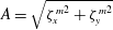$A=\sqrt{{\unicode[STIX]{x1D701}_{x}^{m}}^{2}+{\unicode[STIX]{x1D701}_{y}^{m}}^{2}}$ . $A$ is the maximum displacement that the body can possibly exhibit with amplitudes $\unicode[STIX]{x1D701}_{x}^{m}$ and $\unicode[STIX]{x1D701}_{y}^{m}$ . Iso-contours of $A$ in the ( $\unicode[STIX]{x1D6FD}$ , $U^{\ast }$ ) parameter space are plotted in figure 8(c). The region of large-amplitude vibrations, defined as the region of the parameter space where $A>0.15$ , is indicated in this figure. Large-amplitude vibrations occur over the entire range of $\unicode[STIX]{x1D6FD}$ investigated, even beyond $\unicode[STIX]{x1D6FD}=0.3$ where a steady flow was observed in the fixed body case (§ 3). At low shear, for $\unicode[STIX]{x1D6FD}<0.2$ approximately, large-amplitude vibrations develop on a relatively narrow range of $U^{\ast }$ comparable to that noted in uniform flow. This range rapidly widens around $\unicode[STIX]{x1D6FD}=0.2$ . For $\unicode[STIX]{x1D6FD}\geqslant 0.2$ , large-amplitude vibrations occur up to the maximum reduced velocity considered in this study ( $U^{\ast }=14$ ).

The different regimes of the flow–structure system are explored in the following.

4.2 Flow–structure interaction regimes

Three regimes of the flow–structure system are encountered outside the region of large-amplitude vibrations. Regarding the flow dynamics, these regimes are similar to those previously described in the fixed body case in § 3 (regimes L, H and S), i.e. the flow and fluid forcing features identified in the absence of body motion are not altered by the low-amplitude oscillations. The areas of the parameter space associated with these regimes are indicated in figure 8(c).

To illustrate the persistence of regimes L, H and S in the elastically mounted body case, in the absence of large-amplitude vibrations, the time-averaged value of the in-line force coefficient and its dominant frequency, in selected points of the parameter space (coloured symbols in figure 8 c), are reported in figures 3(a) and 4(a). The results obtained in the fixed and elastically mounted body cases are very close. The slight differences can be attributed to the fact that, in the elastically mounted body case, the existence of a negative time-averaged force in the cross-flow direction induces a shift of the cylinder cross-flow position and thus, a slight modification of the effective Reynolds number and shear parameter seen by the body.

Within the region of large-amplitude vibrations, three other regimes of the flow–structure system are uncovered. These regimes can be clearly identified on the basis of the structural response frequency. The cross-flow response frequency ratio, defined as $f_{y}^{\ast }=f_{y}/f_{nat}$ with $f_{y}$ the dominant frequency of $\unicode[STIX]{x1D701}_{y}$ (based on the Fourier transform of the entire time series), is plotted as a function of $\unicode[STIX]{x1D6FD}$ and $U^{\ast }$ in figure 9; only the points located in the region of large-amplitude vibrations (figure 8 c) are considered in this plot.

Figure 9.

Cross-flow response frequency ratio in the region of large-amplitude vibrations: $f_{y}^{\ast }$ as a function of $U^{\ast }$ , over a range of $\unicode[STIX]{x1D6FD}$ . Typical frequencies of regimes L and H ( $f_{L}=0.16$ and $f_{H}=0.075$ ), normalized by the oscillator natural frequency, are indicated by dashed lines.

Figure 10.

Flow–structure interaction regimes: iso-contours of (a) $f_{y}^{\ast }$ , (b) $\unicode[STIX]{x1D701}_{x}^{m}$ , (c) $\unicode[STIX]{x1D701}_{y}^{m}$ , (d) $C_{x}^{\prime }$ and (e) $C_{y}^{\prime }$ , in the $(\unicode[STIX]{x1D6FD},U^{\ast })$ parameter space. In each plot, the map of the flow–structure interaction regimes is overlaid on the iso-contours. A plain black line delimitates the large-amplitude vibration region. A striped area indicates the region of irregular responses studied in § 4.2.3. Blue symbols denote the points examined in figures 12, 14 and 15.

In the low-shear region ( $\unicode[STIX]{x1D6FD}<0.2$ ), the impact of the shear on the response frequency is limited and the frequencies collapse; the corresponding branch is called VL (i.e. vibratory, low shear). On this branch, the response frequency, close to $f_{L}$ (a typical frequency of regime L, $f_{L}=0.16$ ) at low reduced velocities, deviates from this frequency and gets closer to the oscillator natural frequency ( $f_{y}^{\ast }\approx 1$ ) as $U^{\ast }$ is increased.

In the high-shear region ( $\unicode[STIX]{x1D6FD}\geqslant 0.2$ ), the response frequency generally departs from $f_{L}$ , $f_{H}$ (a typical frequency of regime H, $f_{H}=0.075$ ) and $f_{nat}$ . Two distinct branches appear as functions of the reduced velocity: a low-frequency branch and a high-frequency branch; these branches are referred to as VH1 and VH2 (vibratory, high shear, $1$ and $2$ ). At low reduced velocities (branch VH1), the influence of $\unicode[STIX]{x1D6FD}$ on the response frequency is small. In contrast, the value of the shear parameter is found to have a significant effect on $f_{y}$ close to the transition between branches VH1 and VH2 and in branch VH2.

The regimes occurring in the large-amplitude vibration region are named after the three branches identified above, i.e. VL, VH1 and VH2. The regions of the parameter space associated with these regimes are indicated in figure 10(a), which represents iso-contours of $f_{y}^{\ast }$ . As previously noted (figure 9), each regime exhibits a distinct trend of the oscillation frequency: in regime VL, $f_{y}^{\ast }$ increases as a function of $U^{\ast }$ ; in regime VH1, $f_{y}^{\ast }$ remains close to constant; in regime VH2, $f_{y}^{\ast }$ is larger than in the other regimes, and increases (respectively decreases) as a function of $U^{\ast }$ (respectively $\unicode[STIX]{x1D6FD}$ ). Regimes VL, VH1 and VH2 are characterized by specific properties of the structural responses and fluid forces. To illustrate this aspect, iso-contours of the maximum response amplitudes and r.m.s. values of the fluid force coefficient fluctuations are represented in the $(\unicode[STIX]{x1D6FD},U^{\ast })$ parameter space in figure 10(b–e).

In regime VL, the body cross-flow response and the fluid forces are almost unaltered compared to the uniform current case, relative to the large variations observed at higher shear rates; the in-line oscillation is however substantially amplified.

In both directions, body responses and fluid forces are significantly amplified during the VL–VH1 transition. The peak amplitudes of the body responses and fluid forces are encountered in regime VH1. The structural response amplitudes rapidly decrease during the VH1–VH2 transition. However, the responses are still significant in regime VH2 since the cross-flow oscillation amplitude remains larger than $0.3$ diameters. In regime VH2, the force fluctuations are small in comparison with regimes VL and VH1. Their amplitudes, close to constant, are comparable to and even lower than in the fixed body case, in spite of the vibrations.

The time-averaged in-line force (not plotted here) is generally amplified within the region of large-amplitude vibrations. This explains why the actual time-averaged in-line displacement is usually larger than the estimate based on $\overline{C_{x}}$ in the fixed body case (figure 7 a). The amplification of $\overline{C_{x}}$ is particularly pronounced in regime VH1 where it can reach three times the fixed body case value.

The regimes associated with large-amplitude responses of the body are further investigated hereafter.