


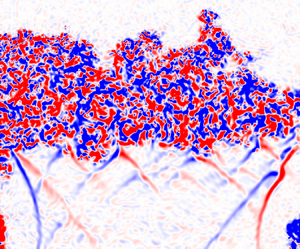





1. Introduction
The Richtmyer–Meshkov instability (RMI) is a fluid instability that occurs when a perturbed interface between two fluids of differing density is impulsively accelerated, usually by a shock wave. The RMI was first described by Richtmyer (Reference Richtmyer1960), and later studied experimentally by Meshkov (Reference Meshkov1969). The interaction of a planar shock wave with perturbations on the interface between the two fluids produces a misalignment of pressure and density gradients that in turn results in the deposition of vorticity at the interface. The flow field induced by this vorticity leads to the formation of spikes of heavy fluid penetrating into the light fluid, and bubbles of light fluid propagating in to the heavy fluid. These spikes and bubbles eventually form mushroom-like structures as they continue to grow. They eventually begin to interact with neighbouring structures, potentially resulting in turbulence and increased mixing between the two fluids (Jacobs & Krivets Reference Jacobs and Krivets2005).
The RMI appears in many notable areas of research ranging from astrophysics to combustion in SCRAMJETs (Arnett et al. Reference Arnett, Bahcall, Kirshner and Woosley1989; Zhou et al. Reference Zhou2021). Most notably, the RMI appears during the implosion stages of inertial confinement fusion (ICF) experiments, such as those performed at the National Ignition Facility (NIF). The ICF experiments at the NIF are performed by irradiating a gold hohlraum with intense laser light resulting in the emission of x-rays that illuminate a spherical capsule containing deuterium–tritium (DT) gas and ice suspended within its centre. The intense x-ray radiation causes the ablation of the capsules’ outer surface, producing an outwards flux of momentum and a corresponding inward directed force that causes the core of the capsule to undergo compression. The laser drive is commonly designed to produce multiple shock waves that are sent through the capsule, interacting with density interfaces formed at the intersection of layers of the different material components forming the capsule and fuel (Lindl, Mccrory & Campbell Reference Lindl, Mccrory and Campbell1992; Lindl et al. Reference Lindl, Landen, Edwards and Moses2014). Importantly, the density interfaces are typically subject to interactions with multiple shock waves originating from both the outer surface of the capsule as well from the reflections of shock waves from the centre of the capsule, resulting in shock wave impacts from both sides of the interfaces. These additional shock wave impacts, initiating a regime known as reshock, drive the RMI to a more energetic turbulent state, resulting in enhanced material mixing. This enhanced mixing in turn leads to an undesirable temperature loss in the plasma core at the centre of the capsule leading to a reduced fusion yield (Smalyuk et al. Reference Smalyuk2019).
Substantial work has been performed to study the RMI in reshock experimentally in various configurations. These have included cases where the interface between the heavy and light gases is initially formed using thin membranes or a splitter plate (Brouillette & Sturtevant Reference Brouillette and Sturtevant1989, Reference Brouillette and Sturtevant1994; Vetter & Sturtevant Reference Vetter and Sturtevant1995; Zaitsev, Titov & Chebotareva Reference Zaitsev, Titov and Chebotareva1996; Puranik et al. Reference Puranik, Oakley, Anderson and Bonazza2004; Leinov et al. Reference Leinov, Sadot, Formoza, Malamud, Elbaz, Levin, Ben-Dor and Shvarts2008, Reference Leinov, Malamud, Elbaz, Levin, Ben-Dor, Shvarts and Sadot2009), membraneless interfaces (Jacobs et al. Reference Jacobs, Krivets, Tsiklashvili and Likhachev2013; Noble et al. Reference Noble, Herzog, Ames, Oakley, Rothamer and Bonazza2020a,Reference Noble, Herzog, Rothamer, Ames, Oakley and Bonazzab; Sewell et al. Reference Sewell, Ferguson, Krivets and Jacobs2021; Noble et al. Reference Noble, Ames, McConnell, Oakley, Rothamer and Bonazza2023), inclined membraneless interfaces (McFarland et al. Reference McFarland, Reilly, Creel, McDonald, Finn and Ranjan2014; Reilly Reference Reilly2015; Mohaghar et al. Reference Mohaghar, Carter, Musci, Reilly, McFarland and Ranjan2017, Reference Mohaghar, Carter, Pathikonda and Ranjan2019) and laminar gas cylinders or gas curtains (Balakumar et al. Reference Balakumar, Orlicz, Tomkins and Prestridge2008a,Reference Balakumar, Orlicz, Tomkins and Prestridgeb; Orlicz et al. Reference Orlicz, Balakumar, Tomkins and Prestridge2009; Balasubramanian et al. Reference Balasubramanian, Orlicz, Prestridge and Balakumar2012; Balakumar et al. Reference Balakumar, Orlicz, Ristorcelli, Balasubramanian, Prestridge and Tomkins2012; Orlicz et al. Reference Orlicz, Balasubramanian, Vorobieff and Prestridge2015). These reshock studies have focused on examining different aspects of the RMI in reshock, including the influence of changing the length of time between the arrival of the incident shock and reshock, the absolute and relative strengths of the incident shock and reshock, and the order of arrival of the two shock waves, as well as examining the ways in which the turbulent nature of the RMI changes following reshock.
One notable aspect of the RMI in reshock is a rapid increase in the growth rate of the mixing layer following the passage of the second shock. Early experiments by Brouillette & Sturtevant (Reference Brouillette and Sturtevant1989) examined the RMI in reshock utilizing a shock tube with a thin membrane initially separating the two gases. In that work, they note a rapid increase in the growth rate of the mixing layer following reshock. Additionally, they found linear growth of the mixing layer with time following reshock, and note that this growth rate appears to decrease following subsequent interactions with additional shock waves. Similar results showing a rapid, although still linear, increase in the growth rate of the mixing layer were found by Brouillette & Sturtevant (Reference Brouillette and Sturtevant1994), Vetter & Sturtevant (Reference Vetter and Sturtevant1995), Zaitsev et al. (Reference Zaitsev, Titov and Chebotareva1996) and Leinov et al. (Reference Leinov, Sadot, Formoza, Malamud, Elbaz, Levin, Ben-Dor and Shvarts2008, Reference Leinov, Malamud, Elbaz, Levin, Ben-Dor, Shvarts and Sadot2009). A linear growth rate of the RMI in reshock was also found by Jacobs et al. (Reference Jacobs, Krivets, Tsiklashvili and Likhachev2013), with those experiments utilizing a membraneless interface technique instead of the membrane used in previous experiments. Linear growth following reshock in membraneless experiments was also observed in the experiments of Mohaghar et al. (Reference Mohaghar, Carter, Musci, Reilly, McFarland and Ranjan2017, Reference Mohaghar, Carter, Pathikonda and Ranjan2019) as well as Noble et al. (Reference Noble, Herzog, Ames, Oakley, Rothamer and Bonazza2020a,Reference Noble, Herzog, Rothamer, Ames, Oakley and Bonazzab). A similar increase in the growth rate following reshock was also found for gas curtain experiments. A potential departure from linear growth at the latest times in reshock was observed by Balakumar et al. (Reference Balakumar, Orlicz, Tomkins and Prestridge2008a), Balakumar et al. (Reference Balakumar, Orlicz, Tomkins and Prestridge2008b), Balakumar et al. (Reference Balakumar, Orlicz, Ristorcelli, Balasubramanian, Prestridge and Tomkins2012) and Balasubramanian et al. (Reference Balasubramanian, Orlicz, Prestridge and Balakumar2012), though only a small number of data points were captured in that regime, making the conclusion of nonlinear growth difficult. Simulations have also found linear growth in reshock (Schilling & Latini Reference Schilling and Latini2010; Lombardini et al. Reference Lombardini, Hill, Pullin and Meiron2011), including simulations with initial perturbations based on experiments (Schilling, Latini & Don Reference Schilling, Latini and Don2007; Latini & Schilling Reference Latini and Schilling2020). A number of models of the RMI in reshock likewise predict linear growth (Richtmyer Reference Richtmyer1960; Brouillette & Sturtevant Reference Brouillette and Sturtevant1989; Mikaelian Reference Mikaelian1989; Charakhch'yan Reference Charakhch'yan2001; Lombardini et al. Reference Lombardini, Hill, Pullin and Meiron2011). Later experiments by Sewell et al. (Reference Sewell, Ferguson, Krivets and Jacobs2021) examined the RMI in reshock with both a low and high amplitude initial perturbation. In contrast with the previous work, those experiments found that the post-reshock mixing layer grew according to a power law of the form  $h\propto t^\theta$, where
 $\theta =0.50\pm 0.07$ and
 $\theta =0.33\pm 0.07$ for the low and high amplitude initial perturbations, respectively. Of particular note, these experiments suggest that, given sufficient time, the RMI in reshock grows with a power law of
 $h \propto t^\theta$ much like the singly shocked RMI. This observation is in agreement with the simulations of Thornber et al. (Reference Thornber, Drikakis, Youngs and Williams2011, Reference Thornber, Drikakis, Youngs and Williams2012), who also found the mixing layer width in reshock to grow with a power law with an exponent of
 $\theta =0.28$ to
 $0.36$. Similar nonlinear growth with a power of
 $2/7 \approx 0.28$ was found by Tritschler et al. (Reference Tritschler, Olson, Lele, Hickel, Hu and Adams2014). Some models also consider nonlinear growth with a power law similar to the singly shocked RMI (Mikaelian Reference Mikaelian2011, Reference Mikaelian2015), while other models permit both linear and power law growth following reshock (Morán-López & Schilling Reference Morán-López and Schilling2013, Reference Morán-López and Schilling2014; Mikaelian & Olson Reference Mikaelian and Olson2020; Schilling Reference Schilling2024). Morán-López & Schilling (Reference Morán-López and Schilling2014) found that a model calibrated to produce power law growth with
 $\theta =0.3$ before reshock best matched the experimental data of Leinov et al. (Reference Leinov, Sadot, Formoza, Malamud, Elbaz, Levin, Ben-Dor and Shvarts2008, Reference Leinov, Malamud, Elbaz, Levin, Ben-Dor, Shvarts and Sadot2009), although these models can be tuned to a range of values of
 $\theta$.
Several experimental studies of the RMI in reshock have considered not only the more typical configuration where the incident shock arrives from the light gas, but also the case where the incident shock arrives from the heavy gas. Brouillette & Sturtevant (Reference Brouillette and Sturtevant1989) utilized a thin membrane to initially separate the two gases in shock tube experiments. This allowed them to form the heavy-over-light interface while also maintaining a thin interface, albeit with the complications associated with the use of a membrane to form the initial interface. They found the interface grew linearly with time, and the growth rate was similar for the two cases. Puranik et al. (Reference Puranik, Oakley, Anderson and Bonazza2004) also considered the case where the incident shock arrives from the heavy gas. In that work, they formed the heavy-over-light interface utilizing a thin plate to initially separate the two gases, with this plate being quickly withdrawn just prior to the experiment. Notably, the heavy-over-light interface was allowed to evolve as a Rayleigh–Taylor unstable layer for a short period of time prior to shock wave arrival. While they did not observe the RMI in reshock, the allowance of Rayleigh–Taylor growth of the mixing layer prior to shock wave arrival does create a similar state to what one might expect in an RMI reshock experiment. In those experiments, they note the phase inversion of the initial perturbations following the passage of the shock wave, which is a phenomenon unique to the heavy incident shock case. They also found qualitative agreement between their mixing layer width versus time measurements and a power law of the form  $h\propto t^\theta$, where
 $\theta =1/3$, though they note that the large amount of scatter in their data makes quantitative assessment difficult. Li et al. (Reference Li, Ding, Si and Luo2020) also considered the case of a heavy-to-light incident shock wave in a convergent geometry. This configuration utilized a soap film to initially separate the heavy and light gases. Notably, each of the experiments that have examined reshock where the incident shock wave arrives from the heavy gas in a single interface RMI experiment have utilized some form of membrane to initially separate the two gases. Membranes that are broken by the arrival of a shock can potentially alter the characteristics of the flow, obscure schlieren and shadowgraph techniques, and make laser-based diagnostics impossible (Jones & Jacobs Reference Jones and Jacobs1997). Therefore, there is utility in examining reshock where the incident shock wave arrives from the heavy gas without the use of membranes or splitter plates.
Studies on the RMI in reshock have also considered how the characteristics of the flow are changed by reshock. This includes rapid increases in the amounts of turbulent kinetic energy (TKE) in the mixing layer, an increase in the Reynolds number and increased material mixing (Zhou Reference Zhou2017b). One particularly notable change is that reshock appears to induce a rapid breakdown of previously ordered structures in the mixing layer following reshock. This has been observed in numerous experiments (Balakumar et al. Reference Balakumar, Orlicz, Tomkins and Prestridge2008a, Reference Balakumar, Orlicz, Ristorcelli, Balasubramanian, Prestridge and Tomkins2012; Balasubramanian et al. Reference Balasubramanian, Orlicz, Prestridge and Balakumar2012; Mohaghar et al. Reference Mohaghar, Carter, Musci, Reilly, McFarland and Ranjan2017, Reference Mohaghar, Carter, Pathikonda and Ranjan2019; Sewell et al. Reference Sewell, Ferguson, Krivets and Jacobs2021), though Balasubramanian et al. (Reference Balasubramanian, Orlicz, Prestridge and Balakumar2012) notes that in their gas curtain experiments there appears to be a persistent imprint of the initial conditions that lasts to late time. Mohaghar et al. (Reference Mohaghar, Carter, Musci, Reilly, McFarland and Ranjan2017) similarly notes that there appears to be a memory of long wavelength initial perturbations following reshock, but little memory of small-scale initial structures. Analysis of the mixing layer following reshock has also demonstrated a rapid transition to turbulence and the formation of an inertial range of scales (Balakumar et al. Reference Balakumar, Orlicz, Tomkins and Prestridge2008a, Reference Balakumar, Orlicz, Ristorcelli, Balasubramanian, Prestridge and Tomkins2012; Schilling & Latini Reference Schilling and Latini2010; Balasubramanian et al. Reference Balasubramanian, Orlicz, Prestridge and Balakumar2012; Mohaghar et al. Reference Mohaghar, Carter, Musci, Reilly, McFarland and Ranjan2017, Reference Mohaghar, Carter, Pathikonda and Ranjan2019; Sewell et al. Reference Sewell, Ferguson, Krivets and Jacobs2021). Balasubramanian et al. (Reference Balasubramanian, Orlicz, Prestridge and Balakumar2012) suggests that an interface with a more complicated structure will also exhibit a more rapid breakdown of coherent structures and increased amounts of mixing following reshock.
A logical extension of the observation of a rapid breakdown of previously ordered structures following reshock is that this may also result in the RMI in reshock more closely resembling isotropic turbulence. This has been examined in simulations (Thornber et al. Reference Thornber, Drikakis, Youngs and Williams2011, Reference Thornber, Drikakis, Youngs and Williams2012; Ristorcelli, Gowardhan & Grinstein Reference Ristorcelli, Gowardhan and Grinstein2013; Tritschler et al. Reference Tritschler, Olson, Lele, Hickel, Hu and Adams2014; Oggian et al. Reference Oggian, Drikakis, Youngs and Williams2015; Thornber et al. Reference Thornber2017; Groom & Thornber Reference Groom and Thornber2018, Reference Groom and Thornber2023), as well as measured in experiments as a function of time (Sewell et al. Reference Sewell, Ferguson, Krivets and Jacobs2021), as a function of space at a small number of fixed time instants (Balakumar et al. Reference Balakumar, Orlicz, Ristorcelli, Balasubramanian, Prestridge and Tomkins2012; Balasubramanian et al. Reference Balasubramanian, Orlicz, Prestridge and Balakumar2012; Mohaghar et al. Reference Mohaghar, Carter, Musci, Reilly, McFarland and Ranjan2017) and through analysis of probability density functions (Orlicz et al. Reference Orlicz, Balasubramanian, Vorobieff and Prestridge2015). Interestingly, there is some disagreement on the late-time trends of anisotropy in the RMI, with some work finding a persistence of anisotropy for a long time following reshock, while others observe a trend towards isotropy at late times after reshock. The anisotropy of the flow as a function of scale size in an RMI mixing layer has also been studied by Mohaghar et al. (Reference Mohaghar, Carter, Musci, Reilly, McFarland and Ranjan2017) as well as Soulard et al. (Reference Soulard, Guillois, Griffond, Sabelnikov and Simoëns2018), where they find a trend towards isotropy for small-scale structures, though large-scale structures remain anisotropic. This rapid breakdown of scales and trends towards isotropy may also suggest that the spectrum of TKE with wavenumber,  $k$, might develop an inertial range with a
 $k^{-5/3}$ Kolmogorov-type scaling, though Zhou (Reference Zhou2001) suggests that an RMI flow may expect to scale closer to
 $k^{-3/2}$, instead. Indeed, both of these scalings have been observed in simulation (Thornber et al. Reference Thornber, Drikakis, Youngs and Williams2011; Tritschler et al. Reference Tritschler, Olson, Lele, Hickel, Hu and Adams2014; Oggian et al. Reference Oggian, Drikakis, Youngs and Williams2015) and experiment (Mohaghar et al. Reference Mohaghar, Carter, Musci, Reilly, McFarland and Ranjan2017, Reference Mohaghar, Carter, Pathikonda and Ranjan2019; Sewell et al. Reference Sewell, Ferguson, Krivets and Jacobs2021).
The influence of changing the time that the RMI is allowed to evolve in the singly shocked regime prior to reshock has been examined in numerous experiments as well. One option to control the length of time between the arrival of the incident shock and reshock is by controlling the length of the region into which the transmitted shock wave propagates after impacting the interface. This has the effect of controlling the time taken for the transmitted shock wave to reflect off of the shock tube end wall and return to the interface to initiate reshock. This was the approach used in the experiments of Leinov et al. (Reference Leinov, Sadot, Formoza, Malamud, Elbaz, Levin, Ben-Dor and Shvarts2008, Reference Leinov, Malamud, Elbaz, Levin, Ben-Dor, Shvarts and Sadot2009), where a false or movable end wall could be adjusted to control the length of the heavy gas portion of the test section, and thereby control the arrival time of reshock at the interface. Balasubramanian et al. (Reference Balasubramanian, Orlicz, Prestridge and Balakumar2012) and Balakumar et al. (Reference Balakumar, Orlicz, Ristorcelli, Balasubramanian, Prestridge and Tomkins2012) likewise varied the shock-to-reshock time in a gas curtain experiment using an adjustable end wall to control the arrival time of the reflected shock wave at the interface. The use of a false end wall has been used in numerous other studies to achieve a desired shock-to-reshock time, even though the studies themselves did not examine the influence of changing this parameter (Balakumar et al. Reference Balakumar, Orlicz, Tomkins and Prestridge2008b; Jacobs et al. Reference Jacobs, Krivets, Tsiklashvili and Likhachev2013; Sewell et al. Reference Sewell, Ferguson, Krivets and Jacobs2021; Zhang et al. Reference Zhang, Zhao, Ding and Luo2023). As will be discussed in more detail in § 2.1, this approach necessarily couples the length of the shock-to-reshock time to the length of the post-reshock observational window and complicates attempts to study a range of shock-to-reshock times while maintaining a long observational window in reshock.
The influence of the reflected shock Mach number on the RMI in reshock has also been studied. The experiments of Leinov et al. (Reference Leinov, Sadot, Formoza, Malamud, Elbaz, Levin, Ben-Dor and Shvarts2008, Reference Leinov, Malamud, Elbaz, Levin, Ben-Dor, Shvarts and Sadot2009) considered the influence of decoupling the strength of the incident and secondary (reshock) shock waves by utilizing compressible foams to remove energy from the reflected shock wave, though the degree of control over the strength of reshock was limited by the range and consistency of available foams. Mohaghar et al. (Reference Mohaghar, Carter, Pathikonda and Ranjan2019) also considered the influence of the shock wave Mach number on the RMI in reshock. In each of these cases, they find that an increase in Mach number results in increased RMI growth rates, the amount of TKE, turbulent mixing and Reynolds numbers, as well as a more rapid transition to turbulence following reshock.
These previous experimental studies provide the context for the goals of this study. The present work has three major goals to examine aspects of the RMI that have previously been difficult to study simultaneously in experiment:
(i) Examine the influence of the order of arrival of the two shock waves on the post-reshock development of the RMI.
(ii) Examine the influence of changing the length of time between the arrival of the incident shock and reshock at the interface on the post-reshock development of the RMI.
(iii) Achieve both of the previous goals with as long of an observational window as is possible in order to examine the development of the RMI at late times after reshock.
This work will be presented in the following sections. Section 2 outlines the experimental configurations and diagnostics used for this work, including a description of the dual driver vertical shock tube (DDVST) used as part of this study. Section 3 describes analysis of the experiments conducted as part of this study, including examination of mixing layer growth rate, rate of TKE decay, Reynolds number and anisotropy of the mixing layer. Finally, § 4 presents the conclusions of this study.
2. Experimental configuration
2.1. Apparatus
The present work has been carried out in a DDVST that has been constructed at the University of Arizona. A solid model representation of this shock tube is shown in figure 1. The DDVST consists of two driver and driven sections oriented on opposite sides of a test section. The lengths of each driver and driven section were optimized so as to achieve the longest period in which the RMI can be observed in reshock within the constraints imposed by cost, laboratory space and manufacturability. This optimized shock tube design consists of a 2.25 m long light driver section, a 3.20 m long light driven section, a 2.23 m long heavy driven section and a 2.36 m long heavy driver section, for a total length of 10 m. The drivers are cylindrical, with a 101.6 mm (4 inch) internal diameter. The driven and test sections are square, with a 88.9 mm (3.5 inch) internal dimension. All tube sections are made of extruded aluminum.
Solid model rendering of the DDVST with section lengths indicated. Also shown is the path of the counterflow gas streams, as well as the location of the diaphragm clamping and forcing mechanisms.

A pneumatic clamping mechanism, used to secure the diaphragms, is located between each driver and driven section. These are indicated as the ‘clamping and forcing mechanism’ in figure 1. The detail view area contains a labelled schematic of this mechanism. The mechanism consists of a rubber bladder located below a plastic ring on one surface, and a metal disk with a compliant rubber gasket on the mating surface. A diaphragm is placed onto the plastic ring, and the driver is lowered onto it. The two surfaces are locked together using a rotating locking ring that is secured using four metal posts. The bladder is then inflated with compressed air to 50 p.s.i., pushing the plastic ring upwards into the mating surface, securing the diaphragm in place. This method for securing the diaphragms was chosen as it provides a greater amount of clamping force and with greater consistency than previous clamping mechanism designs in our lab that use toggle clamps or threaded clamping rings.
This shock tube uses the method of Jones & Jacobs (Reference Jones and Jacobs1997) to form the interface. Streams of heavy and light gases enter the shock tube through the clamping and forcing assembly on the low pressure sides of the diaphragms, with the light gas stream entering at the top of the light driven section, and the heavy gas stream entering at the bottom of the heavy driven section. These gas streams meet at a set of nine 1.6 mm (1/16 inch) diameter holes drilled in the clear test section, where they flow out, forming a stable, stratified interface. The holes remain open during the experiment, and the number and size of the holes was chosen to result in a minimal influence on the development of the RMI. This gas column is then oscillated vertically using a forcing mechanism consisting of a pair of subwoofers attached to the clamping and forcing assembly. The oscillation of the gas column produces Faraday waves that form a semi-random initial perturbation on the interface. The clamping and forcing assembly is shown in greater detail in the detail view of figure 1. Previous work utilizing this forcing method by Jacobs et al. (Reference Jacobs, Krivets, Tsiklashvili and Likhachev2013) as well as Sewell et al. (Reference Sewell, Ferguson, Krivets and Jacobs2021) has shown that the behaviour of the RMI can be influenced by the root-mean-square amplitude of the initial perturbations at the time of incident shock arrival. Additionally, statistical repeatability of the initial perturbations helps to reduce run-to-run variability in the results. To control for these factors, the frequency and amplitude of the sinusoidal signal used to drive the speakers, the length of time that the interface is forced prior to an experiment and the phase of the forcing signal when diaphragm rupture is triggered, is controlled using an Arduino Due microcontroller in order to increase statistical repeatability of the initial perturbations from experiment to experiment.
Figure 2 depicts an  $x$–
 $t$ diagram for a typical experiment in the DDVST. This diagram can be used to trace the progression of an experiment. The main interactions of interest here are as follows:
Points (a,b) The two diaphragms are suddenly ruptured with a controlled time delay between the first and second rupture.
Point (c) The two shock waves arrive at the interface location with a temporal separation that is controlled by the delay between the firing of the two drivers. A number of interactions take place in rapid succession and are depicted in greater detail in the inset of figure 2.
Point (1) The incoming light shock wave impacts the interface, initiating the RMI. This results in a transmitted and reflected shock wave.
Point (2) The transmitted light shock wave then interacts with the incoming heavy shock wave, again producing a reflected and transmitted shock wave.
Point (3) The transmitted heavy shock wave from this interaction then impacts the interface from the opposite side as the initial light shock wave impact, initiating reshock. A transmitted shock wave and a reflected expansion wave are generated from this interaction.
Point (d) The RMI then continues to develop in reshock until the expansion waves that are generated at diaphragm rupture and are subsequently reflected from each driver end wall arrive at the interface location, ending the RMI portion of the experiment.
These interactions highlight how the addition of the second driver provides additional capability to control various aspects of the experiment more simply than would be possible in a single driver design.
The  $x$–
 $t$ diagram corresponding to a dual driver shock tube, with colours added for illustrative purposes. (a) The heavy driver is fired first, emitting the heavy shock wave towards the interface and an expansion wave in to the heavy driver. (b) The light driver is fired a few milliseconds later, emitting the light shock wave towards the interface and an expansion wave in to the light driver. (1) The light shock wave impacts the interface, resulting in a transmitted and reflected shock. (2) This transmitted shock impacts the incoming heavy shock wave, again resulting in a transmitted and reflected shock. (3) The reflected shock from the previous interaction impacts the interface from the opposite direction of the initial impact, initiating reshock. This results in a transmitted shock and reflected expansion wave. (d) The interface has zero bulk interface motion following the second shock until the expansion waves reflected from the ends of the drivers return to the interface.

Firstly, the pressurization of each driver can be independently controlled in a dual driver design, thereby allowing the strength of the shock wave generated by each driver to be specified. This, in turn, allows for the relative strength of the incident shock and reshock, and consequently the post-reshock bulk interface velocity, to be prescribed. The post-reshock bulk interface velocity was chosen to be halted for this study as indicated by the vertical line connecting points (3) and (d) in figure 2, but in practice any post-reshock bulk velocity can be prescribed by controlling the pressurization of the two drivers.
Secondly, the relative time of arrival of the two shock waves at the interface in this design can be controlled by simply delaying the firing of one driver compared with the other. This permits the time between the arrival of the first and second shock waves at the interface to be prescribed. This additionally enables the delay between the firing of the two drivers to be adjusted such that the order of arrival of the two shock waves at the interface may be reversed.
A third strength of the dual driver design is that the driven section containing the heavy gas has been effectively lengthened to include the entirety of the heavy driven section and heavy driver section. The reflected expansion wave produced by the heavy-to-light shock wave impact can be observed near point (3) in figure 2. In a single driver design this expansion wave would travel back in to the heavy gas, reflect off of the end wall of the shock tube and return to the interface, accelerating it and ending the purely RMI portion of the experiment. As the time taken for this expansion wave to return to the interface is related to the same geometry that sets the shock-to-reshock time, it becomes difficult, if not impossible, to decouple the shock-to-reshock time and the length of the post-reshock observational window. In a dual driver design, however, this reflected expansion wave must travel to the end of the heavy driver section and back before it can return to the interface. This process will take significantly longer than the time for the expansion waves from either driver generated at the time of diaphragm rupture to reach the interface. Thus, a dual driver design allows the full length of the heavy driven and driver sections to be available to remove the influence of the reflected expansion wave, thus allowing for a long post-reshock observational window regardless of the shock-to-reshock time of the experiment. A similar set of conditions is true for the case where the incident shock wave arrives from the heavy gas and the second shock wave arrives from the light gas, meaning that a long post-reshock observational window is maintained regardless of the order of shock wave arrival. In practice, the post-reshock observational window lasts approximately  $10$ ms in the DDVST experiments described here. This is a substantially longer period of time than the
 $2$–
 $4$ ms of post-reshock growth that has been possible with the single driver designs used in our laboratory (Jacobs et al. Reference Jacobs, Krivets, Tsiklashvili and Likhachev2013; Sewell et al. Reference Sewell, Ferguson, Krivets and Jacobs2021).
2.2. Experiment description
The experiments presented here have been carried out in three primary experimental groups, totaling 89 experiments. These groups and their relevant parameters are given in table 1. The mean Mach number of the shock wave generated by the light driver is  $M_L = 1.17$ with a standard deviation of
 $\sigma = 0.007$, and the mean Mach number of the shock wave generated by the heavy driver is
 $M_H = 1.18$
 $(\sigma = 0.004)$, with these statistics taken across all experiments presented here. The bulk interface velocity arising from these shock waves is
 $u_{H,I} = 58.68(\sigma =2.14)\, {\rm m}\,{\rm s}^{-1}$ and
 $u_{H,R} = -0.87(\sigma =3.00)\, {\rm m}\,{\rm s}^{-1}$ in the singly shocked and reshocked regimes for the heavy shock first experiments, and
 $u_{L,I} = -61.27~(\sigma =3.80)\, {\rm m}\,{\rm s}^{-1}$ and
 $u_{L,R} = -2.66~(\sigma =1.62)\, {\rm m}\,{\rm s}^{-1}$ in the singly shocked and reshocked regimes for the light shock first experiments, respectively.
List of parameters for the experimental groups in this study.

All experiments in this work utilize air as the light gas and sulfur hexafluoride (SF $_6$) as the heavy gas, yielding an Atwood number of
 $At \equiv (\rho _{SF6} - \rho _{air})/(\rho _{SF6} + \rho _{air}) = 0.67$. Atmospheric pressure and temperature in the laboratory were gathered prior to each experiment using a Bosch BMP280 combination barometer and thermometer. The mean atmospheric pressure was 93.1 (
 $\sigma = 0.25$) kPa and the mean atmospheric temperature was 24.7 (
 $\sigma = 1.1$)
 $^{\circ }$C. These values yield mean densities of
 $\rho _{air} = 1.09\times 10^{-3}$
 $(\sigma =0.01\times 10^{-3})\,{\rm g}\,{\rm cm}^{-3}$ and
 $\rho _{SF6} = 5.49 \times 10^{-3}$
 $(\sigma =0.03\times 10^{-3})\,{\rm g}\,{\rm cm}^{-3}$. The dynamic viscosities of the heavy and light fluids are
 $\mu _H = 1.53\times 10^{-4}\,{\rm g}\,({\rm cm}\,{\rm s})^{-1}$ and
 $\mu _L=1.82\times 10^{-4}\,{\rm g}\,({\rm cm}\,{\rm s})^{-1}$, respectively. An average kinematic viscosity of the two fluids is found as
 $\nu _{avg} = (\mu _H + \mu _L) / (\rho _H + \rho _L) = 0.051\,{\rm cm}^2\,{\rm s}^{-1}$. Suzuki (Reference Suzuki1982) finds the diffusion coefficient of nitrogen and sulfur hexafluoride to be
 $D=0.0945\,\mathrm {cm}^2\,\mathrm {s}^{-1}$. A Schmidt number for air and sulfur hexafluoride in the present experiments is estimated from these quantities as
 $Sc = \nu _{avg} / D \approx 0.54$.
The shock-to-reshock time,  $\Delta t_{s \to rs}$, is a measure of the length of time between the arrival of the incident shock and reshock at the interface. This quantity is varied in this study in order to examine its influence on the post-reshock growth characteristics of the RMI. In addition, both the configuration with the shock wave from the light gas arriving first followed by the shock wave from the heavy gas, as well as the opposite order of arrival of the two shocks, will be considered in this study. Therefore, in order to distinguish the two cases, a positive shock-to-reshock time is defined to indicate the case where the shock wave from the light gas arrives first, followed by reshock from the heavy gas. By similar logic, a negative shock-to-reshock time is defined as the shock wave from the heavy gas arriving first, followed by the shock wave from the light gas.
The length of the shock-to-reshock time period, as well as the Mach numbers of each shock wave, are determined using the output of four PCB Piezotronics 112A22 high-speed pressure transducers, two located in the light driven section and two in the heavy driven section, combined with atmospheric pressure and temperature in the laboratory as measured prior to each experiment. The time that a shock passes each pair of pressure transducers, together with the known spacing of each pressure transducer pair, allows the velocities of both the heavy and light shock waves to be determined for each experiment, and the properties of each gas allow a Mach number of each shock to be calculated. The arrival time of each shock wave at the interface location is calculated from the measured shock wave speeds along with the known distance between the pressure transducers and the interface location. The shock wave that arrives soonest is identified as the incident shock wave. In calculating the arrival time of the second shock wave at the interface, the bulk interface velocity imparted to the interface by the incident shock wave must be accounted for. This is found using the exact Riemann solver presented in Toro (Reference Toro2009). The difference between the arrival times of the two shock waves at the interface are then used to calculate the shock-to-reshock time of each experiment.
The gas properties and measured shock wave strengths described in the previous paragraphs can be used with the exact Riemann solver of Toro (Reference Toro2009) to estimate the change in Atwood number following the impact of the first (incident) and second (reshock) shock waves. A post-incident shock Atwood number of  $At_{H,I} = 0.68(\sigma =0.0005)$ and
 $At_{L,I} = 0.695(\sigma =0.001)$ is found for the heavy and light shock first experiments, respectively. Both groups of experiments have a post-reshock Atwood number of
 $At_{H,R} = At_{L,R} = 0.705(\sigma =0.001)$.
Finally, the cameras used to image the RMI are triggered based on the passage of a shock wave by the pressure transducer closest to the heavy driver section. This transducer is chosen as it is the first to sense a shock wave passage for a wide range of shock-to-reshock times.
2.3. Imaging and diagnostics
The experiments in this work utilize the two-dimensional, two-component particle image velocimetry (PIV) technique to obtain measurements of the velocity field. Particle image velocimetry is a non-intrusive optical diagnostic technique that allows for the reconstruction of a flow field by taking two images of tracer particles seeded into the flow with a known temporal separation. The seeding particles used in this study are vegetable glycerin droplets produced in the seeding apparatus described by Sewell et al. (Reference Sewell, Ferguson, Krivets and Jacobs2021). One apparatus is used for each gas, and the particles are added just before the fluids enter the shock tube. The power applied to each apparatus is controlled so as to generate an appropriate number of particles for PIV. The density of the particles in each gas is attempted to be as closely matched as possible. The particle diameter is approximately  $2\,\mathrm {\mu }{\rm m}$, measured using an in situ measurement based on the acceleration of the particles following the passage of a shock wave (Adrian & Westerweel Reference Adrian and Westerweel2011; Sewell et al. Reference Sewell, Ferguson, Krivets and Jacobs2021). Application of the analysis of Adrian and Westerweel also finds that particles of this size will track the flow with
 $\approx 95\,\%$ accuracy at the maximum temporal frequency resolvable with the present diagnostics.
The experiments presented in this work were captured in three groups corresponding to different configurations of the cameras used to image the experiment. Configurations that utilized multiple cameras were set up such that an overlap of  $\approx 10\,\%$ of the image width existed between the field of view of each camera to facilitate merging of the individual PIV results from each camera into one composite vector field during post-processing. Experimental groups 1 and 2 captured PIV image pairs using a set of four Photron APX-RS Fastcam cameras at a rate of
 $1500$ image pairs per second, with
 $100\,\mathrm {\mu }{\rm s}$ separation between the first and second images in each pair. The cameras in experimental group 1 were arranged in a 2
 $\times$ 2 grid, with each camera capturing a square area with a dimension just over half of the test section width at a resolution of
 $1024 \times 1024$ pixels. This resulted in an approximately square total imaging area with width and height roughly equaling the test section width, yielding a resolution of approximately 1900 pixels across the test section width. This allowed for images to be captured at high resolution, but with the limitation that only a relatively small range of shock-to-reshock times could be visualized. The cameras in experimental group 2 also operated at
 $1024 \times 1024$ pixels, but the cameras were instead oriented in a vertical
 $4\times 1$ stack, with each camera imaging a square area approximately equal to the test section width. This resulted in a spatial resolution that was approximately half of the resolution of group 1, with approximately 1000 pixels across the test section width. The
 $4 \times 1$ orientation, however, allowed for a wider range of shock-to-reshock times to be visualized than was possible in the group 1 configuration. Experimental group 3 utilized a single Phantom v2640. The imaging area was rectangular, and the captured images had a resolution of 1952 pixels in height by 1536 pixels across the test section width, resulting in a slightly lower spatial resolution than the
 $2 \times 2$ camera configuration of experimental group 1. This reduction in resolution was chosen as it allowed the camera to be operated at a much higher imaging rate than was possible with the APX-RS cameras while maintaining the same spatial extents as experimental group 1 and utilizing only a single camera. Additionally, the increased frame rate results in an inter-frame time of
 $1/7500 \approx 133\,\mathrm {\mu }{\rm s}$ between subsequent images, which is similar to the
 $100\,\mathrm {\mu }{\rm s}$ inter-frame time used in experimental groups 1 and 2. This allowed the PIV fields to be calculated using sequential images rather than image pairs as in groups 1 and 2, thereby greatly increasing temporal resolution of the experiments.
The particles within the test section are illuminated by a Photonics Industries DM527-50 70W Nd:YLF high-speed pulsed laser. The laser beam is first focused through the use of a long focal length spherical lens. The beam is then passed through cylindrical lenses to expand it in to a sheet with a height that is sufficient to image the entirety of the camera view(s). The laser sheet then enters the test section through the transparent side wall, perpendicular to the camera views.
The raw image pairs captured from an experiment are post-processed using the PIV post-processing functionality in LaVision's DaVis software in order to reconstruct the flow velocity field. The post-processing in the present work utilizes DaVis's iterative ‘adaptive PIV’ method. This utilizes successively decreasing window sizes, with the results at the previous iteration used to deform the interrogation window of the next iteration to provide more robust results and reduce spurious vector correlations. A final window size of 16  $\times$ 16 pixels with a 75 % overlap was chosen. This results in one velocity field per camera per time instant. If multiple cameras were used for the experiment, each individual velocity field is then merged in to a single composite field that represents the entire observation window.
3. Results
3.1. Interface perturbations
Given the known sensitivity of the behaviour of the RMI to the perturbations on the interface (Zhou Reference Zhou2017b), it is important to quantify the initial interface perturbations in these experiments, including the determination of whether the perturbations are single mode, narrowband or broadband in a spectral sense. These definitions have previously been introduced by Thornber et al. (Reference Thornber, Drikakis, Youngs and Williams2011, Reference Thornber, Drikakis, Youngs and Williams2012) to define an initial interface perturbation spectrum with a single wavelength, a narrow spectral bandwidth or a wide spectral bandwidth, respectively. The spectrum of the initial perturbation in these experiments is quantified by choosing 12 representative experiments that had a relatively large difference in particle seeding density between the heavy and light gases, making the interface between them possible to detect. Ideally, the seeding between the two gases should be similar in order to produce the best PIV data, and so most experiments had well-matched particle seeding densities such that visual interface detection was not possible, limiting the number of experiments that could be analysed in this fashion. Nonetheless, the initial interface spectra from these experiments with a larger difference in seeding density between the two gases should be similar to those with well-matched seeding density. The last image captured prior to the arrival of the incident shock wave is selected from each experiment to best capture the state of the interface at incident shock arrival. A single representative image from this set is shown in figure 3. The initial interface profile is detected utilizing the process described by Sewell et al. (Reference Sewell, Ferguson, Krivets and Jacobs2021) in which a strong Gaussian blurring operation is utilized to make the image intensity in each gas more uniform, and a Sobel edge-detection algorithm is used to identify the interface between the two gases in each column of pixels.
Experimental image depicting the initial perturbations just prior to incident shock arrival. Note that the contrast on this image has been increased to make the initial interface shape easier to identify. The distorted regions on the edge of the image are caused by the exhaust holes in the test section walls.

The spectrum of the initial perturbation for each of the initial interface profiles is found by applying a Hanning window to the profile and then taking the fast Fourier transform (FFT) of each profile, yielding one initial perturbation spectrum per experiment. The magnitude of each Fourier coefficient is then averaged across all 12 chosen experiments to produce a single average initial perturbation spectrum. This averaged spectrum is presented in figure 4 plotted as a function of wavenumber,  $k$. Analysis of this spectrum reveals that
 ${\approx }60\,\%$ of the energy in the initial perturbation spectrum is located at wavenumbers of
 $k \lessapprox 0.7\,2{\rm \pi} \,\mathrm {mm}^{-1}$, with the spectrum being relatively constant in magnitude over this wavenumber range. This range is indicated by the red dashed line in figure 4. The wavenumber range of
 $0.7 \lessapprox k \lessapprox 6.9\,2{\rm \pi} \,\mathrm {mm}^{-1}$ contains another 39 % of the total energy, and the spectrum decays approximately according to
 $k^{-2}$ in this range. This range is indicated by the blue dashed line in figure 4. These two wavenumber ranges therefore contain 99 % of the total energy in this spectrum. A significantly steeper rate of decay is observed for
 $k \gtrapprox 6.9\,2{\rm \pi} \,\mathrm {mm}^{-1}$, with the remaining 1 % of the spectrum energy contained in these scales. Additionally, while this method of quantification of the interface does not capture the diffusion thickness of the two gases, work by Morgan (Reference Morgan2014) in a configuration similar to this one suggests that the diffusion layer should be approximately
 $6$ mm in thickness based on Rayleigh scattering measurements of a flat air–SF
 $_6$ interface.
The averaged spectrum of the initial perturbation of the interface just prior to the arrival of the incident shock. This average is taken across 12 experiments.

This spectrum is slightly steeper than the  $\sim k^{-1.5}$ spectrum found in the experiments of Sewell et al. (Reference Sewell, Ferguson, Krivets and Jacobs2021) that was also used as the initial conditions for the simulations of Groom & Thornber (Reference Groom and Thornber2023). Those simulations also considered initial spectra of the form
 $k^{-0.5}$ and
 $k^{-1}$. The present perturbation spectrum is also steeper than the
 $k^{-1}$ utilized for the simulations of Thornber et al. (Reference Thornber, Drikakis, Youngs and Williams2011). The jet-based initial condition of Weber et al. (Reference Weber, Haehn, Oakley, Rothamer and Bonazza2014) (and others in that facility (Reese et al. Reference Reese, Oakley, Navarro-Nunez, Rothamer, Weber and Bonazza2014, Reference Reese, Ames, Noble, Oakley, Rothamer and Bonazza2018; Noble et al. Reference Noble, Herzog, Ames, Oakley, Rothamer and Bonazza2020a,Reference Noble, Herzog, Rothamer, Ames, Oakley and Bonazzab, Reference Noble, Ames, McConnell, Oakley, Rothamer and Bonazza2023)) had a spectrum based on scalar variance that was proportional to
 $k^{-1}$ at low wavenumbers and transitions to a
 $k^{-3}$ and later
 $k^{-5}$ decay at middle and high wavenumbers in their experiments. A relatively flat low wavenumber component and a
 $\sim k^{-2}$ spectrum at higher wavenumbers was also observed in the (tilt-compensated) initial condition of Mohaghar et al. (Reference Mohaghar, Carter, Musci, Reilly, McFarland and Ranjan2017, Reference Mohaghar, Carter, Pathikonda and Ranjan2019), with this spectrum similarly based on scalar fluctuations. Finally, gas curtain experiments have a much more regular and single-mode interface owing to the method of their formation (Jacobs Reference Jacobs1993; Jacobs et al. Reference Jacobs, Klein, Jenkins and Benjamin1993, Reference Jacobs, Jenkins, Klein and Benjamin1995; Balakumar et al. Reference Balakumar, Orlicz, Tomkins and Prestridge2008a,Reference Balakumar, Orlicz, Tomkins and Prestridgeb; Orlicz et al. Reference Orlicz, Balakumar, Tomkins and Prestridge2009; Balakumar et al. Reference Balakumar, Orlicz, Ristorcelli, Balasubramanian, Prestridge and Tomkins2012; Balasubramanian et al. Reference Balasubramanian, Orlicz, Prestridge and Balakumar2012; Orlicz et al. Reference Orlicz, Balasubramanian, Vorobieff and Prestridge2015).
3.2. Experimental progression
As discussed in previous sections, the PIV technique utilized in this work only resolves the velocity field of this flow as opposed to a concentration or density field. Therefore, methods of assessing the state and evolution of the RMI must be similarly velocity based. One useful metric for a velocity-based analysis is the magnitude of the component of vorticity normal to the image plane,  $\omega = ( \boldsymbol {\nabla } \times \boldsymbol {u} ) \boldsymbol {\cdot } \hat {n}$. Considering that the passage of a shock wave through the interface results in deposited vorticity, and that there is no mean vorticity elsewhere in the test section, this metric will naturally highlight the regions where RMI-induced vorticity is present. Vorticity is calculated in the present work using the DaVis software package in which the gradients are calculated using a central difference scheme involving the four closest neighbours (i.e. the vectors above, below, left and right) of a given vector.
A montage of vorticity pseudocolour plots from an example experiment is shown in figure 5. The experiment presented in this montage is a heavy shock first experiment from experimental group 2. These composite images are the result of merging the individual PIV vector fields from four cameras oriented in a vertical stack to form one composite vector field. The experimental images used to generate these fields are captured at a rate of 1500 image pairs per second. Therefore, the time between each image in this montage is  $1/1500 \approx 0.66$ ms.
A montage of PIV fields resulting from images captured during a single heavy shock first experiment from experimental group 2. The colour scale is shown at the bottom of the figure and is fixed across all images. Times of each image relative to reshock are (a)  $-$2.90 ms, (b)
 $-$2.23 ms, (c)
 $-$1.56 ms, (d)
 $-$0.90 ms, (e)
 $-$0.23 ms, ( f) 0.43 ms, (g) 1.10 ms, (h) 1.76 ms, (i) 2.43 ms, ( j) 3.10 ms, (k) 3.76 ms, (l) 4.43 ms, (m) 5.10 ms, (n) 5.76 ms, (o) 6.43 ms, (p) 7.10 ms, (q) 7.76 ms, (r) 8.43 ms.

The interface location is initially at the bottom of the viewable area, which is indicated by the dashed line in figure 5(a). The interface is then impacted by the incident shock wave in figure 5(b), travelling upward from the heavy gas into the light gas, causing the interface to travel upward and initiating the RMI in the incident shock regime. The RMI then develops in figure 5(b–e) as the interface continues to travel upwards in the tube. The interface is impacted a second time by the shock wave arriving from the light gas travelling downwards into the heavy gas in figure 5( f), with this impact taking place approximately  $\Delta t_{s \to rs} = 3.0$ ms after the incident shock arrival. The second shock wave arrival initiates the RMI in the reshock regime, as indicated by the increased intensity of vorticity on this fixed colour scale and the development of finer scales of turbulent motion as compared with the pre-reshock flow. This rapid transition from relatively ordered structures pre-reshock to a more disorganized structure has been observed in previous experiments (Balakumar et al. Reference Balakumar, Orlicz, Tomkins and Prestridge2008a, Reference Balakumar, Orlicz, Ristorcelli, Balasubramanian, Prestridge and Tomkins2012; Balasubramanian et al. Reference Balasubramanian, Orlicz, Prestridge and Balakumar2012; Mohaghar et al. Reference Mohaghar, Carter, Musci, Reilly, McFarland and Ranjan2017, Reference Mohaghar, Carter, Pathikonda and Ranjan2019; Sewell et al. Reference Sewell, Ferguson, Krivets and Jacobs2021). The RMI is then allowed to evolve in the reshock regime in figure 5(g–r). It can be observed that the bulk interface velocity is approximately halted, and the mixing layer is stationary in space as it evolves following the second shock interaction. Some large-scale structures may be observed in these images, though the randomness in the initial perturbation results in the spatial distribution of these larger structures being different for each experiment. The RMI continues to evolve in reshock for approximately 8 ms in this experiment. During this time, viscosity acts to dissipate energy in the mixing layer, indicated by the decreasing colour intensity on the fixed colour scale used here.
Aside from the RMI itself, there are a number of other features observable in figure 5 that are interesting to note. One immediately noticeable feature is the apparent thickness of the shock waves observed in the images. This occurs due to the transit of the shock wave between the first and second images in the PIV image pair. A similar phenomenon was also observed by Sewell et al. (Reference Sewell, Ferguson, Krivets and Jacobs2021).
Another feature worth pointing out in these images are the noticeable lines of vorticity lying below the mixing layer following reshock. There are both larger diagonal lines approximately the width of the test section, as well as smaller wedge-like structures visible. These lines of vorticity represent vortex sheets produced by velocity shear across the slip lines connected to triple points formed as the refracted shock wave passes through the mixing layer. The largest structures that span the test section width as well as the dome-shaped structures near the left and right walls are likely caused by the interaction of the incident shock wave with the boundary layers along the shock tube walls. These vortex sheets persist for the remainder of the experiment observation time. The smaller vortex sheets appear to be correlated with the location of the largest structures in the mixing layer at the time of reshock, suggesting that they are formed by the refraction of the shock wave as it transits the mixing layer. These structures are quickly obscured by the growing mixing layer shortly following reshock.
A final observation of importance in these images is the presence and growth of boundary layers on the side walls of the test section. The boundary layers are visible in these images as the camera fields of view capture the flow all the way to the test section walls. The boundary layers are initially very thin such that they are not visible in the incident shock regime and become significantly thicker, as well as potentially transitioning to turbulence, following reshock. This is more noticeable in the heavy gas region owing to the significantly lower kinematic viscosity there, resulting in a larger Reynolds number.
3.3. Mixing layer width
An important measurement in the study of the RMI is the growth of the width of the mixing layer versus time. Normally, the mixing layer width is defined by a concentration distribution of the two gases. However, as discussed above, the PIV diagnostic only resolves the velocity field and so methods for detecting the mixing layer must similarly be velocity based.
Sewell et al. (Reference Sewell, Ferguson, Krivets and Jacobs2021) used a method that identified the mixing layer as the region where spanwise-averaged TKE is greater than 5 % of its maximum value. A similar approach is utilized here to determine the extent of the mixing layer using elevated levels of spanwise-averaged plane normal enstrophy instead of TKE. Enstrophy was chosen for this work over TKE as the fact that there is no mean shear in this flow makes the separation of the fluctuating part of the field unnecessary and simplifies this stage of analysis. Spanwise averaging is required for this stage of the analysis as the changing shock-to-reshock times of these experiments, the run-to-run variation in shock wave strengths and the lack of density or concentration measurements make the methods for spatially aligning the results across different experiments for ensemble averaging imprecise. Previous simulations by Groom & Thornber (Reference Groom and Thornber2023) have shown that the mixing layer width defined using TKE will tend to be larger than the volume fraction based mixing layer width. Given that the enstrophy-based metric used in this work is similarly based on velocity, it is reasonable to expect that these mixing layer widths are also greater than the volume fraction based mixing layer width.
The mixing layer is identified through a series of steps. Figure 6 illustrates this automated process of identifying the mixing layer for a single frame in a single experiment. Figure 6(a) shows the vorticity field output from PIV processing. The left and right  $2$-
 $3$ mm of the field is cropped to remove edge effects near the shock tube walls (black dashed line), with the cropped area set by the specific camera configuration used for the experiment. The image-plane normal component of vorticity is then squared to obtain enstrophy (
 $\omega ^2$), shown in figure 6(b). This enstrophy field is then averaged along the
 $x$ axis to generate a one-dimensional spanwise-averaged profile as shown in figure 6(c). Note that this profile has elevated values where the mixing layer is located and low values elsewhere. A boxcar moving average with a window size of 10 points (
 ${\approx }3$ mm) of the spanwise-averaged profile is then taken to smooth the fluctuations in the data, shown as the red line in figure 6(d). This step is done to reduce the influence of noise in the data on the detection of the edge of the mixing layer, and provides smoother overall results. The maximum value of this smoothed profile and its corresponding position is then found, indicated by the green vertical line in figure 6(c). The search for the maximum value is restricted to a region visually identified as the mixing layer in the vorticity pseudocolour images, with this step performed to increase the robustness of the automated algorithm against random imperfections in the data far away from the mixing layer location (e.g. a small pocket of unseeded gas drifting into the camera view). Finally, the edges of the mixing layer are found by starting at the location of this maximum value and marching outwards until the value of the smoothed profile is less than 5 % of the maximum value. These locations, indicated by the pink and blue vertical lines in figure 6(c), are used to define the edges of the mixing layer, and the mixing layer width is defined as the distance between these edges. The influence of the choice of the 5 % threshold used here on the mixing layer width results is discussed in Appendix A.
(a) A single vorticity field from a PIV experiment. (b) Enstrophy field calculated from the vorticity field in (a). (c) The resulting row-averaged enstrophy profile. (d) Moving average profile (red) and locations of maximum value and mixing layer edges associated with moving average dropping below 5 % of the maximum value.

The result of this width finding process for a single experiment is shown as the black dots in figure 7. Note that this data appears to follow a power law of the form  $h(t) \propto t^\theta$ (Alon et al. Reference Alon, Hecht, Mukamel and Shvarts1994). The parameter
 $\theta$ is found in the present work by plotting the logarithm of width versus the logarithm of time and fitting a line to the result. It should be acknowledged that utilizing a fit of this form implicitly assumes that
 $h=0$ at
 $t=0$, which is clearly not the case here, but is necessary due to complications that arise from attempting to fit a more general model equation that accounts for this discrepancy (e.g.
 $(h-h_0) = a (t - t_0)^\theta$) where unique solutions are often difficult to obtain. As a consequence, these fits focus on late-time data where the influence of this assumption is small. The result of this fit is shown in figure 7 using the red dashed line, which yields a value of
 $\theta = 0.314 \pm 0.025$ at 95 % confidence for this particular experiment. Points early in the experiment were excluded from this fit as these points do not appear to be well described by the model equation.
Measured interface mixing layer width from a single PIV experiment with a shock-to-reshock time of  $\Delta t_{s\to rs}=2.0\,{\rm ms}$ on (a) linear and (b) log–log axes. The red line indicates the fit of
 $h(t) \propto t^\theta$ to the data, where
 $\theta = 0.314 \pm 0.025$ (95 %) is found for this experiment. Data points indicated by a black cross were excluded from the fit and points indicated by a blue cross in (a) correspond to the incident shock regime.

Prior studies have suggested a wide range of values for  $\theta$, from as high as 2/3 (Barenblatt Reference Barenblatt1983) to as low as 0.18 (Zhou Reference Zhou2017a), though many of these studies did not consider the reshock case. As noted in § 1, a great deal of previous experimental work, models and simulations have observed or predicted linear growth of the RMI in reshock, making the observation of power law growth behaviour of the RMI in reshock in these experiments noteworthy. Other work has found power law growth of the RMI in reshock. Simulations by Tritschler et al. (Reference Tritschler, Olson, Lele, Hickel, Hu and Adams2014) found power law growth of the RMI in reshock where
 $\theta = 2/7 \approx 0.285$, while Thornber et al. (Reference Thornber, Drikakis, Youngs and Williams2011) found
 $\theta$ in the range of 0.28 for narrow bandwidth initial conditions to 0.36 for broad bandwidth initial conditions. Power law growth of the RMI in reshock in an experiment was observed by Sewell et al. (Reference Sewell, Ferguson, Krivets and Jacobs2021), who found values of
 $\theta$ between 0.33 and 0.5 in reshock for high and low amplitude experiments, respectively. Power law growth of the reshocked RMI has also been predicted by models (Mikaelian Reference Mikaelian2011; Morán-López & Schilling Reference Morán-López and Schilling2013, Reference Morán-López and Schilling2014; Mikaelian Reference Mikaelian2015; Mikaelian & Olson Reference Mikaelian and Olson2020; Schilling Reference Schilling2024). The present experiments generally agree well with this previous work, particularly the broad bandwidth simulations of Thornber et al. (Reference Thornber, Drikakis, Youngs and Williams2011), as well as the high amplitude initial perturbation experiments of Sewell et al. (Reference Sewell, Ferguson, Krivets and Jacobs2021). The simulations of Groom & Thornber (Reference Groom and Thornber2023), which were based on the shock tube experiments of Sewell et al., have found that
 $\theta$ found from a velocity-based mixing layer width agreed well with those based on integral or volume fraction based measurements, particularly for relatively broadband initial conditions as in these experiments.
Given the capabilities of the DDVST it is interesting to consider how the value of  $\theta$ varies with shock-to-reshock time. The result of this process is shown in figure 8. The black dots shown are the values of
 $\theta$ found from fits of individual experiments, and the error bars show the 95 % confidence interval of the fits. Only fits that have
 $N>4$ points and
 $r^2 > 0.75$ are included in this plot to remove experiments with too little data to properly fit the model equation and which would yield large confidence intervals, as well as cases where the fit poorly describes the data. These fits show a significant amount of scatter owing to the sensitivity of the curve fitting process. Overall, despite this scatter, the average values of
 $\theta$ obtained from the heavy shock first experiments appear to be very similar to values obtained from the light shock first experiments. Furthermore, if it is assumed that the value of
 $\theta$ is, in an average sense, constant for each set of experiments, but that it has a different value for heavy shock first and light shock first experiments, a comparison can be made of the two cases. An average value of
 $\theta _{avg,H} = 0.365 \pm 0.018$ (95 %) is found for the heavy shock first experiments and
 $\theta _{avg,L} = 0.381 \pm 0.020$ (95 %) is found for the light shock first experiments. The standard deviation of the values of
 $\theta$ is
 $0.082$ and
 $0.057$ for the heavy shock first and light shock first experiments, respectively. In this comparison, the 95 % confidence interval is the uncertainty of the mean owing to data scatter, and does not include the uncertainty in the fits of each constituent measurement. The average value of
 $\theta$ for the heavy shock first cases is indicated by the red dashed line in figure 8, and for the light shock first cases by the blue dashed lines on figure 8. The shaded areas indicate the 95 % confidence bound of the respective mean values. The average value of these two cases are similar, and both averages lie within the 95 % confidence interval of the other average. This result is qualitatively in agreement with the results of Brouillette & Sturtevant (Reference Brouillette and Sturtevant1989), who found that the heavy and light shock first experiments had slightly different linear growth rates but that these differences were also within the uncertainty bounds. Previous experiments by Sewell et al. (Reference Sewell, Ferguson, Krivets and Jacobs2021) found
 $\theta =0.33\pm 0.07$ and
 $\theta =0.50\pm 0.07$ in reshock for their high and low amplitude initial perturbation, respectively. The present work agrees well with the high amplitude results, though the value of
 $\theta$ is slightly lower than the low amplitude initial perturbation results. Additionally, the relatively short post-reshock observational period in those results could also influence this comparison. The simulations of Thornber et al. (Reference Thornber, Drikakis, Youngs and Williams2011, Reference Thornber, Drikakis, Youngs and Williams2012) found
 $\theta =0.28$ to
 $\theta =0.36$ for narrowband and broadband initial conditions, respectively, with the latter case agreeing well with the relatively broadband perturbations in these experiments.
Values of  $\theta$ found via a linear least-squares fit of enstrophy width for each experiment versus that experiment's shock-to-reshock time. The horizontal lines indicate average values of
 $\theta$, separated by heavy shock first and light shock first experiments, and the shaded areas represent the 95 % confidence interval of the associated mean.

3.4. Rate of decay of TKE
Many turbulent flows have a constant source of energy input such that the amount of TKE per unit mass will grow with time until eventually the rate of energy addition is matched by the rate that it is dissipated by viscosity. This is not the case with RMI, in which the entirety of the energy is added as the shock wave passes through the interface. The energy then freely decays in time until it is entirely dissipated by viscosity. For this reason, it is useful to examine the total amount of TKE within the mixing layer as it decreases with time and the rate at which this energy decays.
The TKE per unit mass is calculated from the fluctuating components of the turbulent velocity. Variables in turbulent flows can be decomposed in to a mean component plus a component representing fluctuations about that mean. Therefore, the total velocity resolved by the PIV diagnostic must be decomposed into its mean and fluctuating components in order to calculate TKE. In uniform density flows this is performed using the Reynolds decomposition, defined as  $f = \bar {f} + f'$, where
 $\bar {f}$ is the mean and
 $f'$ is the fluctuations of
 $f$ about
 $\bar {f}$. For non-uniform density flows, such as the RMI, this decomposition is instead commonly performed using the Favre, or mass-weighted, decomposition to account for spatial variations in density. Importantly, however, the Favre decomposition requires the density field that can not be obtained using the PIV diagnostic, and so the Reynolds decomposition must be used for the present analysis. It should be noted that variable density flows introduce a number of complexities to a turbulent flow stemming from the non-uniform density field (Charonko & Prestridge Reference Charonko and Prestridge2017; Lai, Charonko & Prestridge Reference Lai, Charonko and Prestridge2018). As a consequence, the influence of Reynolds averaging on these results should be considered. Work by Mohaghar et al. (Reference Mohaghar, Carter, Musci, Reilly, McFarland and Ranjan2017) as well as Charonko & Prestridge (Reference Charonko and Prestridge2017) has shown that while a Reynolds averaging approximation does introduce a small error versus a Favre average, this difference is only a few percent of the total value. The TKE is defined here as one half of the trace of the Reynolds stress tensor (Pope Reference Pope2000). The TKE corresponding to the three components of the flow velocity is
 \begin{equation} k_u = \tfrac{1}{2}(u - \bar{u})^2 = u^{'2},\quad k_v = \tfrac{1}{2}(v - \bar{v})^2 = v^{'2},\quad k_w = \tfrac{1}{2}(w - \bar{w})^2 = w^{'2}, \end{equation}
where the mean part of each velocity component is defined as the average value of that velocity component within the mixing layer. This method of determining the mean flow was chosen due to the difficulties associated with ensemble averaging noted in § 3.3. The TKE field is defined in terms of these components as
 \begin{equation} K = k_u + k_v + k_w. \end{equation}
Another aspect to consider in this analysis is that the two-dimensional PIV technique used in this study does not resolve the out-of-plane horizontal component of velocity,  $w$. To address this, an assumption is made that, in a statistical sense, the in-plane (resolved) horizontal component of fluctuating velocity is similar to the out-of-plane (unresolved) horizontal component of fluctuating velocity, i.e.
 $u' \approx w'$. This assumption has been used in other experiments with a two-dimensional PIV diagnostic to account for the out-of-plane component of velocity (Mohaghar et al. Reference Mohaghar, Carter, Musci, Reilly, McFarland and Ranjan2017, Reference Mohaghar, Carter, Pathikonda and Ranjan2019; Sewell et al. Reference Sewell, Ferguson, Krivets and Jacobs2021). The assumption of statistical homogeneity along the horizontal axes in RMI flows is common in simulations (for example, Thornber et al. Reference Thornber, Drikakis, Youngs and Williams2011, Reference Thornber, Drikakis, Youngs and Williams2012; Tritschler et al. Reference Tritschler, Olson, Lele, Hickel, Hu and Adams2014; Oggian et al. Reference Oggian, Drikakis, Youngs and Williams2015; Groom & Thornber Reference Groom and Thornber2018, Reference Groom and Thornber2019, Reference Groom and Thornber2023). Therefore, TKE in this study is defined as
 \begin{equation} K = 2 k_u + k_v. \end{equation}
Volume integrated specific TKE is then calculated by integrating  $K$ over the mixing layer,
 \begin{equation} \frac{E_{tot}}{\bar{\rho}} = L_z \iint K\,{{\rm d}\kern0.06em x}\,{{\rm d} y}, \end{equation}
where  $L_z=88.9$ mm is the out-of-plane depth of the test section and
 $x$ and
 $y$ are the cross-stream and streamwise directions as indicated in figure 6. Volume integrated specific TKE is used here due to the lack of density measurements in these experiments. The decay of volume integrated specific TKE is presented in log–log form for a single experiment in figure 9. Here the black dots represent the value of
 $E_{tot}$ at each time instance for this particular experiment. The experimental data appears to fall in a straight line on this log–log plot, suggesting that the volume integrated specific TKE in the mixing layer decays according to a power law. Thus, a form for this decay of
 $E_{tot} \propto t^p$ will be assumed, where
 $a$ and
 $p$ are coefficients to be found from a fit to the data. The fit is performed identically to the fit of mixing layer width versus time described above, with the data plotted as
 $\log (E_{tot})$ vs
 $\log (t)$ and a straight line fit to the result. The fit for this particular experiment is indicated by the red dashed line, and has a slope of
 $p = -0.834$ with a 95 % confidence interval of the fitted value of
 $\pm 0.077$.
Volume integrated specific TKE versus time for a single PIV experiment on (a) linear and (b) log–log axes. The red dashed line indicates a fit of  $E_{tot} \propto t^p$ to the data, where
 $p=-0.834 \pm 0.077$ at 95 % confidence for this experiment. Black crosses indicate data points that were excluded from the fit.

Thornber et al. (Reference Thornber, Drikakis, Youngs and Williams2010) has shown that the decay exponent of TKE,  $p$, for RMI can be related to the growth exponent,
 $\theta$, deriving the expression
 $p = 3 \theta _{tke} - 2$, where the subscript in
 $\theta _{tke}$ is meant to differentiate this value of
 $\theta$ from the one found from the mixing layer width. A similar result for volume integrated TKE was also found by Schilling (Reference Schilling2021). This allows a comparison between these results and those in § 3.3, though it should be noted that the definition of TKE used by Thornber et al. (Reference Thornber, Drikakis, Youngs and Williams2010) to find
 $\theta$ from TKE decay contains a spatially varying density profile, whereas the present results do not have this density data available. The experiment shown in figure 9, for example, has a fitted slope of TKE decay of
 $p = -0.834\pm 0.077$, which corresponds to
 $\theta _{tke} = (-0.834\pm 0.077 + 2)/3 \approx 0.388 \pm 0.026$.
As with the mixing layer width measurements, it is interesting to consider the effect of shock-to-reshock time on the volume integrated specific TKE decay rate. Figure 10 shows values of the slope of volume integrated specific TKE decay,  $p$, versus shock-to-reshock time indicated by the black dots along with the equivalent values of
 $\theta _{tke} = (p + 2)/3$ on the right axis. As in figure 8, the 95 % confidence interval of each fit is indicated by the error bars. There is again a significant amount of scatter that can be observed in this data. However, the amount of scatter along with the size of the error bars are noticeably smaller than was observed for the width-based measurements in figure 8. A major source of uncertainty in the mixing layer width measurements is believed to arise from the emergence of large-scale flow structures, such as a single large mushroom ejected from the mixing layer. The mixing layer width finding process will detect the emergence of these larger structures as the edge of the mixing layer and, consequently, the measurement of mixing layer width will be overly influenced by these structures. Thus, one might expect a larger run-to-run variation in
 $\theta$ measurements depending on the presence of the larger structures. On the other hand, the total amount of TKE, and the rate at which it decays, is arguably less influenced by the emergence of new structures in the flow. This results in less run-to-run variation in the volume integrated specific TKE decay measurements, as well as less uncertainty in the fit of the data from each experiment.
Values of the rate of TKE decay and corresponding values of  $\theta _{tke}$ found via a linear least-squares fit of volume integrated specific TKE in the mixing layer versus time for each experiment versus that experiment's shock-to-reshock time. The horizontal lines indicate average values of
 $p$, separated by heavy shock first and light shock first experiments, and the shaded areas represent the 95 % confidence interval of the associated mean.

Similar to as was done for the mixing layer growth exponent, the assumption may be made that  $p$ has a constant value for the heavy shock first and light shock first experiments, but that these values may be different for the two cases. This allows a mean, and associated 95 % confidence interval of that mean, to be found for each of the two groups of experiments. The mean value for the heavy shock first experiments is indicated by the red dashed line and for the light shock first experiments is indicated by the blue dashed line in figure 10. The 95 % confidence intervals of each mean are indicated by the shaded areas. The rate of decay of volume integrated specific TKE for the heavy shock first experiments is found to be
 $p_{avg,H} = -0.823 \pm 0.06$ (95 %) and, for the light shock first experiments,
 $p_{avg,L} = -1.061 \pm 0.032$ (95 %). The standard deviation in the values of
 $p$ is
 $0.175$ and
 $0.127$ for the heavy shock first and light shock first experiments, respectively. As with the average values of
 $\theta$ from mixing layer width measurements, the 95 % confidence interval here arises from the 95 % confidence of the mean and does not include the uncertainty of the fit of the constituent points. These average values of
 $p$ correspond to values of
 $\theta _{tke}$ of
 $\theta _{tke,avg,H} = 0.392 \pm 0.02$ (95 %) and
 $\theta _{tke,avg,L} = 0.313 \pm 0.011$ (95 %) for the heavy and light shock first experiments, respectively. Notably, the 95 % confidence interval of
 $\theta _{tke,avg,H}$ overlaps with the 95 % confidence band of
 $\theta _{avg,H} = 0.365 \pm 0.018$ from the mixing layer width in the heavy shock first case, though a similar overlap is not observed in the light shock first case. Note that the average values of
 $p$ found here are more negative than the values of
 $p_{high} = -0.62$ and
 $p_{low} = -0.14$ for high and low amplitude initial conditions found by Sewell et al. (Reference Sewell, Ferguson, Krivets and Jacobs2021), though this is likely at least in part due to the much longer post-reshock observational window in these experiments. One important difference between figures 10 and 8 is that there is now a significant difference between the heavy shock first and light shock first volume integrated specific TKE decay measurements and that this difference exceeds the 95 % confidence values of the mean.
It is important to recognize that the difference in the values of  $p$ between the two groups could be the result of the lack of density/concentration measurements in these experiments. Recall in (3.4) that (1) Favre averaging was not used when calculating the TKE field, and (2) a density field is not used in calculating the TKE. As a consequence, there is an implicit assumption that the relationship between the distributions of density and velocity over time is the same for the light shock first and heavy shock first cases. It should also be noted that the influence of variable density effects may also produce different behaviours in the heavy shock first and light shock first cases and contribute to this observed behaviour (Charonko & Prestridge Reference Charonko and Prestridge2017; Lai et al. Reference Lai, Charonko and Prestridge2018). Further examination of the rate of decay of TKE in this configuration, particularly where the first shock arrives from the heavy gas, via simulation, or experiment with the addition of density measurements, would help clarify this.
3.5. Reynolds number
The Reynolds number is a dimensionless parameter defined as the ratio of inertial to viscous forces, commonly defined in RMI type flows as  ${\textit {Re}} = h \dot {h} / \nu$, though alternative definitions have been proposed for different phases of RMI growth (Orlicz et al. Reference Orlicz, Balasubramanian, Vorobieff and Prestridge2015). Here,
 $h$ is the mixing layer width,
 $\dot {h}$ is the growth rate of the mixing layer and
 $\nu = \nu _{avg}$ is the average kinematic viscosity of the two pure fluids on either side of the mixing layer. Each of these quantities can be found through known properties of the two pure fluids (
 $\rho$ and
 $\mu$,
 $\therefore \nu _{avg}$) or from direct measurements of the data (
 $h$,
 $\dot {h}$). The determination of the growth rate,
 $\dot {h}$ is complicated slightly by the fact that it requires taking a derivative of noisy experimental data, which in turn tends to result in still noisier derivatives. This is somewhat mitigated in this work by using a line fit to multiple neighbouring points to determine
 $\dot {h}$, which will smooth the high frequency noise in the Reynolds number while retaining the low frequency behaviour, though noisy results remain a consistent issue.
Figure 11 shows a plot of Reynolds number versus time for a single experiment. Note that there are large fluctuations in the value of the Reynolds number observed in this plot that is due to the use of a numerical derivative of noisy data as discussed above. The Reynolds number is  ${\textit {Re}} \approx 6 \times 10^4$ shortly after reshock in this case, and decays to a somewhat smaller value of
 ${\textit {Re}} \approx 3\times 10^4$ towards the end of the experiment, though the scatter in the data makes a precise value difficult to determine. Two reference lines are also indicated on this plot. The red dashed line arises from a fit of a power law of the form
 ${\textit {Re}} \propto t^r$ to this data, where
 $r=-0.20$ is the fitted value. The blue dotted line arises from the expected decay of Reynolds number with time arising from the assumption of self-similarity (i.e.
 $h \propto t^\theta$,
 ${\textit {Re}} = h \dot {h}/\nu _{avg} \therefore {\textit {Re}}_\theta \propto t^{2\theta -1}$), where a value of
 $\theta =0.37$ is used based on the average value of
 $\theta$ found in figure 8.
Reynolds number versus time for a single experiment with a shock-to-reshock time of  $\Delta t_{s \to rs} = -0.76$ ms. The red dashed line indicates a fit of a power law of the form
 $a t^r$ to the data, where
 $a=5.79\times 10^4$ and
 $r=-0.20$. The blue dotted line indicates the expected decay of the Reynolds number assuming self-similarity (i.e.
 $h \propto t^\theta$,
 ${\textit {Re}} = h \dot {h}/\nu _{avg} \therefore {\textit {Re}}_\theta \propto t^{2\theta -1}$), where
 $\theta =0.37$.

In order to assess the effect of shock-to-reshock time, the value of the Reynolds number may also be examined in a similar manner to as how the influence of the shock-to-reshock time on mixing layer growth and volume integrated specific TKE decay were analysed. An average Reynolds number may be found for each experiment by taking the average of all data points in the first  $5$ ms following reshock. An uncertainty in this value can also be calculated from the uncertainty of the mean, which captures the influence of the level of noise present in the underlying data as well as the decay in the value of the Reynolds number over the 5 ms window. Figure 12 shows this average value of the Reynolds number for each experiment versus that experiment's shock-to-reshock time. The error bars indicate the associated 95 % confidence interval of the value of the average. It can be observed in this figure that experiments with shorter shock-to-reshock times of
 $|\Delta t_{s \to rs}| \lessapprox 1.0$ ms demonstrate a sharp decrease in average Reynolds number as shock-to-reshock time decreases, approaching a minimum at simultaneous shock and reshock arrival, i.e. when
 $\Delta t_{s \to rs}$ approaches zero. Some experiments in this limit were observed to demonstrate a very low growth of the mixing layer, with this behaviour attributed to the cancellation of vorticity owing to the short period of time between the arrival of the incident and secondary shock waves (Mikaelian Reference Mikaelian1985, Reference Mikaelian1989). An example of such an experiment in the present dataset is presented in Appendix B. In contrast, experiments with a shock-to-reshock time of
 $|\Delta t_{s \to rs}| \gtrapprox 1.0$ ms achieve a similar average value of the Reynolds number of
 ${\textit {Re}}_{avg} \approx 1 \times 10^5$, with this value observed across a range of shock-to-reshock times. While the observed trend towards a minimum value of average Reynolds number for small shock-to-reshock times is unsurprising as one may expect less growth of the mixing layer in this limit, it is interesting to note that the Reynolds number does not continue to increase with increasing shock-to-reshock time for
 $|\Delta t_{s \to rs}| > 1.0$ ms. A possible explanation for this behaviour is that the growth of short wavelength perturbations in the incident shock regime saturate relatively quickly. This would result in the amplitudes of the perturbations just prior to reshock changing relatively little beyond a certain shock-to-reshock time, and this may in turn result in relatively little change of the post-reshock Reynolds number as well. Finally, the post-reshock outer-scale Reynolds number appears to be insensitive to the order of arrival of the two shock waves, with experiments having both positive and negative values of shock-to-reshock time achieving approximately the same value of average Reynolds number.
Average value of Reynolds number versus shock-to-reshock time for the first  $5$ ms post-reshock. Error bars represent the 95 % confidence interval of the mean. The blue and red lines indicate the suggested critical Reynolds numbers for transition to turbulence from Dimotakis (Reference Dimotakis2000) and Zhou (Reference Zhou2007), respectively.

The Reynolds number is a useful metric to establish whether these experiments have achieved a fully turbulent state. Dimotakis (Reference Dimotakis2000) indicates that an outer-scale Reynolds number with a value greater than  ${\textit {Re}} > 1 \times 10^4$ is required in order to achieve the transition to turbulent mixing, with this relationship having been found by considering a number of different turbulent flows, not just the RMI. Zhou (Reference Zhou2007) suggests a critical Reynolds number for the transition to turbulent mixing to be
 $1.6 \times 10^5$ for time-dependent laboratory-scale flows. This value was determined by calculating the minimum Reynolds number required to generate an inertial range with sufficient separation between the large and small scales such that some part of the developing inertial range would be unaffected by either the largest or smallest scales of the flow. These critical values suggested by Dimotakis and Zhou are indicated in figure 12 by the blue and red lines, respectively. The Reynolds numbers observed in the present study are in excess of the Reynolds number suggested by Dimotakis. On the other hand, the average Reynolds number for most experiments in the present study fall below the value suggested by Zhou. This suggests that while the present experiments may be approaching a turbulent state, they are not ‘fully turbulent’ according to the definition provided by Zhou (Reference Zhou2007).
3.6. Turbulent length scales
Another method to assess the degree to which a flow is turbulent involves estimating the size of the largest and smallest scales in the inertial range. The present work considers the scales defined by Dimotakis (Reference Dimotakis2000) and Zhou, Robey & Buckingham (Reference Zhou, Robey and Buckingham2003), which are given by
 \begin{equation} \left. \begin{aligned} &\lambda_L \simeq 5 \textit{Re}^{{-}1/2} h ,\\ &\lambda_D \simeq C (\nu t)^{1/2} ,\\ &\lambda_\nu \simeq 50 \textit{Re}^{{-}3/4} h ,\\ &\lambda_K \simeq \textit{Re}^{{-}3/4} h ,\\ \end{aligned} \right\} \end{equation}
where these scales are in order of decreasing size for a fully turbulent flow. Here,  $\lambda _L$ is the Liepmann–Taylor scale,
 $\lambda _D$ is the time-dependent outer-scale viscous shear layer scale,
 $\lambda _\nu$ is the inner viscous scale and
 $\lambda _K$ is the Kolmogorov scale.
These length scales may be utilized to quantify the transition to turbulence in several ways. Three possible criteria will be considered here. The first criterion is  $\lambda _L > \lambda _\nu$, suggested by Dimotakis (Reference Dimotakis2000), and is arrived at by noting that the largest scales in the inertial range,
 $\lambda _L$, must be greater than the smallest scales in the inertial range,
 $\lambda _\nu$, in order to have an inertial range and, thus, fully developed turbulence. The second criterion is the Zhou–Robey criterion,
 $\lambda _{L,min} \equiv \min (\lambda _L, \lambda _D) > \lambda _\nu$, defined by noting that the time-dependent outer-scale viscous shear layer scale,
 $\lambda _D$, introduced by Zhou et al. (Reference Zhou, Robey and Buckingham2003) adds an additional scale by which the upper bound of the inertial range may be specified. Therefore, Zhou et al. defined the upper bound of the inertial range to be the smaller of the two scales. The time dependence of
 $\lambda _D$ and, therefore, of this transition criterion, is of particular note as it suggests that a transition to turbulence can still occur even after the shock wave has passed through the interface and the RMI has begun to decay due to the time needed to form these scales of motion. Third, Lombardini, Pullin & Meiron (Reference Lombardini, Pullin and Meiron2012) suggests that the ratio required for a full separation of scales and transition to turbulence is
 $\lambda _L / \lambda _\nu \geq 10$, and notes that this threshold was only met for
 $M \geq 3$ in their simulations.
Estimates of the turbulent length scales given in (3.5) were computed for all experiments presented in this work. The length scale size estimates for experiments with a shock-to-reshock time of  $|\Delta t_{s \to rs}| > 1.0$ ms are shown pointwise in figure 13(a) and in a moving average sense in figure 13(b). The length scale size estimates for experiments with a shock-to-reshock time of
 $|\Delta t_{s\to rs}| > 1.0$ ms are shown pointwise in figure 13(c) and in a moving average sense in figure 13(d). Also shown in figure 13(b,d) are estimated length scale sizes based on the assumption of self-similarity (i.e.
 $h \propto t^\theta$,
 ${\textit {Re}} = h \dot {h}/\nu _{avg} \therefore {\textit {Re}}_\theta \propto t^{2\theta -1}$) in (3.5), where a value of
 $\theta =0.37$ is used based on the average value of
 $\theta$ found in figure 8. Notably, the average length scales do appear to be well described by the self-similar growth assumption, particularly at middle to late times in the experiment.
Length scale size versus time for experiments where (a,b)  $1.0 \geq |\Delta t_{s \to rs}| > 0.3$ ms and (c,d)
 $|\Delta t_{s \to rs}| > 1.0$ ms, in a (a,c) pointwise and (b,d) moving average sense. Colours correspond to
 $h$ (black),
 $\lambda _L$ (red),
 $\lambda _\nu$ (blue),
 $\lambda _D$ (green) and
 $\lambda _K$ (cyan). The window size of the moving average is
 $1/1500$ s. The coloured dashed lines in (b) and (d) indicate predicted length scales based on self-similarity (i.e.
 $h\propto t^\theta, {\textit {Re}}={\textit {Re}}_\theta$) where
 $\theta =0.37$, and the horizontal black dashed line indicates the average experimental resolution,
 $\Delta x_{avg} = 0.27\,\textrm {mm}\,\textrm {vector}^{-1}$.

As described above, there are three transition criteria to consider when viewing this data. It is clearly observable for both groups of experiments in figure 13, particularly in the moving average sense, that the transition criterion of Dimotakis is satisfied for the duration of the experiment, though the experiments with a short shock-to-reshock time have noticeably less separation between these two scales than the experiments with a long shock-to-reshock time. The moving average data for the experiments with a short shock-to-reshock time suggests that the Zhou–Robey transition criteria is not satisfied for this group of experiments. In contrast, the experiments with a long shock-to-reshock time do satisfy the Zhou–Robey transition criteria for a short period of time, approximately 3–4 ms after reshock. The pointwise data, however, shows that individual experiments in both groups may satisfy this transition criteria for a longer period of time than the moving average data would suggest. It is important to note, however, that even though the Zhou–Robey transition criteria is satisfied, there is only minimal separation between the largest and smallest scales in the inertial range. The third criterion is  $\lambda _L / \lambda _\nu > 10$ as suggested by Lombardini et al. (Reference Lombardini, Pullin and Meiron2012). This ratio is found to be between approximately 1.5 and 1.8 for experiments with a short and long shock-to-reshock time, respectively, and so does not satisfy this criterion. It should be noted, however, that Orlicz et al. (Reference Orlicz, Balasubramanian, Vorobieff and Prestridge2015) finds almost an order of magnitude difference in estimates of
 $\lambda _L / \lambda _\nu$ in their gas curtain experiments depending on whether these length scales were estimated from the outer-scale Reynolds number or from measured values of the Taylor and Kolmogorov length scales and relationships between these scales and
 $\lambda _L$ and
 $\lambda _\nu$. They note that this ambiguity could lead to different conclusions depending on the scaling used, indicating ambiguity in the definition of a transition to turbulence using only Reynolds numbers. Thus, further analysis via the spectra of flow scales is useful to examine if, and to what degree, this flow has formed an inertial range of scales.
3.7. Spectrum of TKE
The spectrum of TKE is a tool by which the energy content of a turbulent flow as a function of scale size may be examined. One method by which the TKE spectrum may be calculated is through the use of the FFT algorithm. The procedure used here for calculating this spectrum for a single time instance follows the one described by Latini, Schilling & Don (Reference Latini, Schilling and Don2007), except that the calculations in this case are not weighted by density. This is also similar to the calculation performed by Sewell et al. (Reference Sewell, Ferguson, Krivets and Jacobs2021). The FFT of the fluctuating part of each component of velocity is taken in the  $x$ direction, across the test section, at each
 $y$ position in the mixing layer. The component FFTs are then multiplied by their complex conjugates to obtain the spectrum of each component of TKE,
 \begin{equation} \widehat{k_u} = \widehat{u^{'}}\widehat{u^{'}}^*,\quad \widehat{k_v} = \widehat{v^{'}}\widehat{v^{'}}^*, \end{equation}
where  $\widehat {k_u}$ is the spectrum of TKE magnitude of the horizontal component of velocity,
 $u$,
 $\widehat {({\cdot })}$ indicates a Fourier transform and
 $({\cdot })^*$ indicates a complex conjugate. A similar definition for the vertical component of velocity,
 $\widehat {k_v}$ is also defined. The values from each velocity component are then combined to form the TKE spectrum as
 \begin{equation} \hat{K} = \left( 2 \widehat{k_u} + \widehat{k_v} \right), \end{equation}
where the factor of  $2$ on
 $\widehat {k_u}$ is used to account for the out-of-plane component of horizontal velocity, which is assumed to be similar to the in-plane component. This follows similar logic as that used for adding the factor of
 $2$ to the
 $u$ component of TKE in the calculation of volume integrated specific TKE in § 3.4. This process is then repeated for all
 $y$ positions in the mixing layer to obtain one TKE spectrum per
 $y$ position. The magnitude of each Fourier coefficient is then averaged at each wavenumber across the mixing layer, resulting in an average one-dimensional TKE spectrum for each time instant,
 \begin{equation} \bar{\hat{K}} = \left(\overline{ 2 \widehat{k_u} + \widehat{k_v} } \right), \end{equation}
where  $\overline {( {\cdot } )}$ indicates an average over the mixing layer. These spectra are further ensemble averaged across groups of experiments, with ensemble averages indicated using angle brackets,
 $\langle {\cdot } \rangle$. In order to ascertain the effects of the shock-to-reshock time and the order of arrival of the two shock waves on the spectrum of TKE, the present experimental results are divided into four groups. These groups correspond to a large negative shock-to-reshock time (
 $\Delta t_{s \to rs} \leq -1.0$ ms), a small negative shock-to-reshock time (
 $-1.0 < \Delta t_{s \to rs} \leq -0.3$ ms), a small positive shock-to-reshock time (
 $0.3 \leq \Delta t_{s \to rs} < 1.0$ ms) and a large positive shock-to-reshock time (
 $\Delta t_{s \to rs} \geq 1.0$ ms). An ensemble average of the anisotropy ratio of the experiments in each group are then taken, with ensemble averages indicated using angle brackets,
 $\langle {\cdot } \rangle$. The ensemble average is calculated using a boxcar moving average to translate all experimental data points on to a common set of time and wavenumber coordinates. In addition, this process only averages the data that falls within a specified window of time and wavenumber about a given point, and no interpolation of the data is performed. The half-width of the temporal window is
 $1/3000$ s, corresponding to a total temporal window size equivalent to the lowest imaging frame rate of 1500 frames per second. The half-width of the wavenumber window is
 ${\rm \pi} 115 / 85\,\textrm {mm}^{-1}$, corresponding to half of the spectral resolution of the lowest resolution experiments. The range of wavenumbers used in these averages is likewise limited to the resolvable range of the lowest resolution experiments. Each TKE spectrum from each experiment is normalized by the total energy of the spectrum prior to averaging.
The ensemble-averaged spectrum of TKE, compensated by the Kolmogorov  $k^{-5/3}$ scaling, over the four ranges of shock-to-reshock time are presented in figure 14. This compensation results in regions of the spectra that follow a Kolmogorov-type
 $k^{-5/3}$ scaling with wavenumber appearing as a flat, horizontal line. A fiducial representing a
 $k^{-3/2}$ type spectrum as suggested by Zhou (Reference Zhou2001) is also shown in each plot as a red dashed line. Each greyscale line represents the ensemble-averaged TKE amplitude spectrum for a single time instant in the ensemble. The grey value of each line represents the length of time elapsed past reshock, with black representing the latest time in the experiment.
Ensemble-averaged compensated spectra for four groups of experiments. These four groups correspond to (a) large negative, (b) small negative, (c) large positive and (d) small positive shock-to-reshock times. The red dashed lines indicate a  $-3/2$ slope of decay of TKE with wavenumber as suggested by Zhou (Reference Zhou2001), and the blue dashed lines indicate a Kolmogorov
 $-5/3$ slope of decay.

There are several aspects of note in the plots shown in figure 14. First, all four groups of experiments exhibit a  $\approx -3/2$ type scaling at early times after reshock, in agreement with the suggested decay rate for an RMI-induced turbulent flow of Zhou (Reference Zhou2001). The experiments with a longer shock-to-reshock time (plots a,c) then shift towards a
 $\approx -5/3$ decay rate at later times in the experiment as indicated by the TKE spectrum flattening and becoming horizontal over time in these compensated plots. Interestingly, such a shift in the spectral content of the mixing layer is not observed for experiments with a shorter shock-to-reshock time (plots b,d), where a
 $\approx -3/2$ spectrum is maintained for the duration of the experiment. These observations are consistent with the observation from figure 13 that shows the scales representing the upper and lower bounds of the inertial range are beginning to separate in the experiments with longer shock-to-reshock times, while such a separation is not as evident in experiments with shorter shock-to-reshock times. The appearance of nearly a decade of wavenumbers following a
 $k^{-5/3}$ decay at later times in the long shock-to-reshock time experiments is interesting to note, as this indicates the formation of an inertial range of scales and a transition to turbulence that was not suggested by the Reynolds number or length scale analyses in §§ 3.5 and 3.6. This echoes the ambiguity noted by Orlicz et al. (Reference Orlicz, Balasubramanian, Vorobieff and Prestridge2015) who suggested that an RMI flow may not be ‘fully turbulent’ as defined by a Reynolds number-based analysis while at the same time the turbulent spectra indicate the formation of an inertial range of scales, suggesting the flow is in fact ‘fully turbulent.’ Similar results depicting a
 $k^{-5/3}$ decay of TKE have been noted in other experiments (Mohaghar et al. Reference Mohaghar, Carter, Musci, Reilly, McFarland and Ranjan2017; Sewell et al. Reference Sewell, Ferguson, Krivets and Jacobs2021), though a slightly steeper rate of decay of
 $-1.8$ to
 $-2.2$ was found by Mohaghar et al. (Reference Mohaghar, Carter, Pathikonda and Ranjan2019). A
 $k^{-3/2}$ to
 $k^{-5/3}$ decay has also been observed in simulation (Thornber et al. Reference Thornber, Drikakis, Youngs and Williams2011; Tritschler et al. Reference Tritschler, Olson, Lele, Hickel, Hu and Adams2014; Oggian et al. Reference Oggian, Drikakis, Youngs and Williams2015).
3.8. Anisotropy
Isotropy is often considered of importance in many turbulent flows, and turbulence is often studied under the idealization of a homogeneous, isotropic turbulent flow (Kolmogorov Reference Kolmogorov1991a,Reference Kolmogorovb). However, many flow phenomena, such as the RMI, are inherently anisotropic by virtue of their physical configuration, having mean density, pressure or velocity gradients that exist in only one direction. The degree of anisotropy in a reshocked RMI mixing layer has been studied in a number of simulations and experiments as noted in § 1. There is some disagreement in the overall trends of anisotropy versus time in these studies. Simulations by Thornber et al. (Reference Thornber, Drikakis, Youngs and Williams2011) found that the mixing layer remains anisotropic at late times after reshock, with a different asymptotic degree of anisotropy for broadband and narrowband initial conditions. Groom & Thornber (Reference Groom and Thornber2018) observed a trend towards isotropy in their simulations, but found the flow nonetheless remains anisotropic for a long time following reshock. Sewell et al. (Reference Sewell, Ferguson, Krivets and Jacobs2021) found the mixing layer to be initially strongly anisotropic following reshock and decreasing anisotropy over time, though the experiment did not extend late enough following reshock to observe steady-state behaviour. Other studies, such as those of Balakumar et al. (Reference Balakumar, Orlicz, Ristorcelli, Balasubramanian, Prestridge and Tomkins2012), Balasubramanian et al. (Reference Balasubramanian, Orlicz, Prestridge and Balakumar2012) and Orlicz et al. (Reference Orlicz, Balasubramanian, Vorobieff and Prestridge2015) found a late-time trend towards isotropy for the RMI mixing layer. It is therefore of interest in the present work to examine the temporal trends of anisotropy and how these trends change with shock-to-reshock time.
The anisotropy of the RMI may be quantified in more than one way. One common measure of anisotropy is the anisotropy ratio, which is defined as the ratio of the sum of the vertical and horizontal components of TKE. This may be defined in three dimensions in cases where all three components of velocity are available (Cook, Cabot & Miller Reference Cook, Cabot and Miller2004); however, the present experiments resolve only two components of velocity, and so the two-dimensional definition of Thornber et al. (Reference Thornber, Drikakis, Youngs and Williams2011) will be used instead,
 \begin{equation} A_R = \frac{\sum k_v }{ \sum k_u }, \end{equation}
where the summations are over all values within the mixing layer. An isotropic state is represented by  $A_R=1$, with
 $A_R>1$ indicating more energy in the vertical direction than the horizontal and
 $A_R<1$ indicating more energy in the horizontal direction than the vertical.
In order to ascertain the effects of the shock-to-reshock time and the order of arrival of the two shock waves on anisotropy, the present experimental results are divided in to the same four groups based on shock-to-reshock time as presented in figure 14. The ensemble average is calculated using a boxcar moving average to translate all experimental data points on to a common set of coordinates. The moving average window has a half-width of  $1/3000$ s, corresponding to a total window size equivalent to the slowest imaging frame rate across all of the present experiments. In addition, this process only averages the data that falls within a specified window of time about a given point, and no interpolation of the data is performed. The resulting ensemble-averaged anisotropy ratio of the four groups is shown in figure 15. Also shown for comparison are horizontal bands representing asymptotic values of
 $A_R = 1.8 \pm 0.2$ and
 $A_R = 1.7 \pm 0.1$ found from the simulations by Thornber et al. (Reference Thornber, Drikakis, Youngs and Williams2011) for broadband and narrowband initial conditions, respectively.
Anisotropy ratio versus time for four groupings of experiments corresponding to large negative, small negative, small positive and large positive shock-to-reshock times. Shaded areas indicate the range of anisotropy ratio found from simulation (Thornber et al. Reference Thornber, Drikakis, Youngs and Williams2011).

Several trends may be observed in the data in figure 15. The mixing layer for all four groups begins initially very anisotropic with vertical TKE significantly exceeding horizontal TKE. The anisotropy for all four groups then trends towards, although does not reach, an isotropic state at early times following reshock. The experimental groups with the longest shock-to-reshock times demonstrate a more rapid trend towards isotropy than those with a shorter shock-to-reshock time. No significant difference is observed between the heavy shock first and light shock first cases with similar shock-to-reshock times. All four groups reach a minimum anisotropy ratio of approximately 1.1. The four groups all reach a nearly equal degree of anisotropy at around 3-4 ms after reshock, and demonstrate increasing anisotropy for the remainder of the experiment. The experiments approach a quasi-steady value of  $1.6 \lessapprox A_R \lessapprox 1.8$ at the latest times, although the length of time that this quasi-steady value is observable is relatively short. The experiments with the longest positive shock-to-reshock time approach a quasi-steady value of
 $A_R \approx 1.8$, and the experiments with the shortest shock-to-reshock time approach a quasi-steady value of
 $A_R \approx 1.6$ for both the heavy and light shock first cases. The heavy shock first experiments with the longest shock-to-reshock times do not appear to approach a quasi-steady value by the end of these experiments.
The data presented in figure 15 suggest that, while experiments with a longer shock-to-reshock time approach an isotropic state more rapidly than those with a shorter shock-to-reshock time, there does not appear to be an influence of the order of arrival of the two shock waves. This result suggests that the degree of anisotropy of the mixing layer is primarily influenced by the length of the shock-to-reshock time, and the direction of traversal of reshock does not appear to have a significant influence on the post-reshock degree of anisotropy. The tendency for experiments with a long shock-to-reshock time to more rapidly approach an isotropic state after reshock compared with those with a short shock-to-reshock time is consistent with the simulations of Ristorcelli et al. (Reference Ristorcelli, Gowardhan and Grinstein2013), who found that an increase in mixing layer width prior to reshock, which is equivalent to an increased shock-to-reshock time here, would result in a decrease in the degree of anisotropy in a reshocked mixing layer, although they did not examine the heavy shock first case. Additionally, at later times ( $t \gtrapprox 3.0$ ms) in the present experiments there appears to be only limited influence of the shock-to-reshock time and the order of arrival of the two shock waves, with all four groups demonstrating a similar degree of anisotropy with the primary difference between the four groups being the quasi-steady value obtained at the end of the experiments.
There is a notable qualitative departure in behaviour of anisotropy ratio versus time between the data presented in figure 15 and data presented by Thornber et al. (Reference Thornber, Drikakis, Youngs and Williams2011) as well as summarized by Zhou (Reference Zhou2017b) (and others presented within that work). The quasi-steady values of  $A_R \approx 1.6-1.8$ obtained from the present experiments at the latest times generally agree with the results found in simulations by Thornber. However, those simulations show qualitatively different temporal behaviour of anisotropy, with the value of the anisotropy ratio approaching its final value monotonically without the initial dip and subsequent increase observed in the present experiments. There has been other work that shows a qualitatively similar behaviour of anisotropy versus time as is observed here, with anisotropy ratio approaching a minimum value at early times, followed by an increase at later times (Ristorcelli et al. Reference Ristorcelli, Gowardhan and Grinstein2013; Oggian et al. Reference Oggian, Drikakis, Youngs and Williams2015; Soulard et al. Reference Soulard, Guillois, Griffond, Sabelnikov and Simoëns2018). The reasons for this behaviour may be related to changes in the dominance of small and large scales of the flow over time. Kolmogorov (Reference Kolmogorov1991b) suggests that a turbulent flow should become isotropic at small scales. Mohaghar et al. (Reference Mohaghar, Carter, Musci, Reilly, McFarland and Ranjan2017) finds that, at late time, the small-scale components of the flow do indeed trend towards isotropy. Soulard et al. (Reference Soulard, Guillois, Griffond, Sabelnikov and Simoëns2018) suggests further that an RMI flow with a decreasing amount of energy in the large scales should become increasingly isotropic, and that a trend towards isotropy in the RMI appears to be driven by the emergence of small-scale flow structures. It may be argued from these suggestions that the behaviour observed in the present experiments is the result of a change in the energy content of the smallest relative to the largest scales in the flow, and the difference in the isotropy of those scales, as the RMI develops in reshock. To further develop this idea, it is useful to consider the spectrum of anisotropy to examine anisotropy as a function of scale size.
The spectrum of anisotropy is calculated in a similar manner to the spectrum of TKE discussed previously in § 3.7. Equation (3.6a,b) is again used to calculate the spectrum of TKE for each component of velocity. In this case, however, each component is treated separately instead of being combined to form a single TKE spectrum. The spectra  $\overline {\widehat {k_u}}$ and
 $\overline {\widehat {k_v}}$, corresponding to the spectrum of TKE in the horizontal and vertical directions from (3.6a,b), are calculated and the average spectrum across the mixing layer is found for each component. The ratio of these two average spectra is then calculated on a per-wavenumber basis to obtain a value of the anisotropy ratio as a function of wavenumber,
 \begin{equation} \widehat{A_R} = \frac{\overline{\widehat{k_v}}}{\overline{\widehat{k_u}}}, \end{equation}
where  $\hat {A}_R$ is the spectrum of the anisotropy ratio. This can be viewed as the equivalent of (3.9) in a spectral sense. The anisotropy ratio spectra are then ensemble averaged in the same manner as the TKE spectra. Plots of this ensemble-averaged anisotropy ratio spectrum versus wavenumber for the same four groups of experiments shown in figure 14 is presented in figure 16. Again, each curve in the plot has a grey value corresponding to the time of the curve relative to reshock, with black representing the latest times in the experiment.
Anisotropy versus wavenumber for four groups of experiments: (a) large negative, (b) small negative, (c) large positive and (d) small positive shock-to-reshock times. The red dashed line in each plot is a reference line indicating isotropy.

It is observed in these plots that, in agreement with the results of Mohaghar et al. (Reference Mohaghar, Carter, Musci, Reilly, McFarland and Ranjan2017) as well as Soulard et al. (Reference Soulard, Guillois, Griffond, Sabelnikov and Simoëns2018), the lowest wavenumber contributions to this flow appear to be anisotropic, while the higher wavenumber contributions trend towards isotropy. Experiments with a long shock-to-reshock time (plots a,c) appear to show a time dependence of the anisotropy at low wavenumbers, with the longer wavelength components initially isotropic, but becoming increasingly anisotropic with time. There does not appear to be any similar temporal trend at high wavenumber, however. Very little time dependence is observed over all wavelengths of the spectrum in the short shock-to-reshock time groups (plots b,d). Additionally, only the length of the shock-to-reshock time, and not the order of shock wave arrival, appears to influence these observed behaviours.
Finally, it is worth considering whether the observed scale dependence of the anisotropy ratio as shown in figure 16, together with the shift in scale sizes as a function of time shown in figures 13 and 14, can be utilized to explain the change in anisotropy ratio as a function of time shown in figure 15. To do this, the centroid wavenumber of the ensemble-averaged TKE spectra are calculated at each time in the ensemble. The value of the anisotropy ratio at the centroid wavenumber is found from the spectrum of anisotropy at the same time in the ensemble. This quantity will be termed the spectral centroid anisotropy ratio and written as  $A_{R,c}$ to differentiate it from the anisotropy ratio defined in (3.9). The plot of the spectral centroid anisotropy ratio versus time calculated using this approach is shown in figure 17. It is notable that, although the values of the spectral centroid anisotropy ratio found using this method are slightly less than those found in figure 15, the temporal trends are similar. This indicates that the trends in the anisotropy ratio versus time observed in figure 15 do appear to be at least partially explained by the change in the dominance of different scales of the flow, as well as the anisotropy of those scales, over time.
Spectral centroid anisotropy ratio versus time for four groups of experiments. This is calculated by finding the centroid of the ensemble-averaged TKE spectrum in figure 14 at each time instant, and then finding the corresponding value of anisotropy ratio for that time instant and centroid location from the ensemble-averaged anisotropy spectrum in figure 16.

4. Conclusions
Experiments on the turbulent RMI in a novel DDVST have been presented. These experiments, and the corresponding analysis, span a wide range of shock-to-reshock times, including reversing the order of arrival of the two shock waves. The experiments have a duration of approximately 10 ms after reshock, allowing ample time for trends in the RMI over time to be quantified. The shock wave strengths from the two gases were chosen so as to result in arrested bulk interface motion following reshock.
Several metrics of interest to the RMI are examined for the influence of the shock-to-reshock time on their value. The first is the value of the mixing layer growth exponent,  $\theta$. The mixing layer growth was observed to grow consistent with a power law of the form
 $h(t)\propto t^\theta$ following reshock. No significant difference in the value of
 $\theta$ was observed across a range of shock-to-reshock times, excluding very short shock-to-reshock times. An average value of the growth exponent for heavy shock first experiments of
 $\theta _H = 0.365 \pm 0.018$ (95 %) and for light shock first experiments of
 $\theta _L = 0.381 \pm 0.02$ (95 %) is found. A significant amount of scatter is observed in the value of
 $\theta$ between individual experiments, however. These average values generally agree with the value of
 $\theta \approx 0.33$ found by Sewell et al. (Reference Sewell, Ferguson, Krivets and Jacobs2021) for the high amplitude reshocked case. Thornber et al. (Reference Thornber, Drikakis, Youngs and Williams2011) found
 $\theta$ in the range of 0.28 for narrow bandwidth initial perturbations to 0.36 for broad bandwidth initial perturbations. The latter result is in good agreement with the results presented here, which also have a relatively broadband initial perturbation.
Another metric of interest included in this study is the rate of decay of volume integrated specific TKE versus time, and the dependence of this value on the shock-to-reshock time. When fitting a power law for volume integrated specific TKE decay of the form  $E_{tot} / \bar {\rho } \propto t^p$, an average value of the decay constant of
 $p_H = -0.823 \pm 0.06$ (95 %) is found for the heavy shock first experiments and
 $p_L = -1.061 \pm 0.032$ (95 %) for the light shock first experiments. Notably, the 95 % confidence interval of the average value of
 $p$ for the light shock first experiments lies outside of the 95 % confidence interval of the heavy shock first result. This suggests that, on average, the TKE decay constant has a statistically significant dependence on the order of shock wave arrival. A possible explanation for the difference between the heavy shock first and light shock first experiments is offered by considering that TKE as defined in this work does not include density and, thus, includes an implicit assumption that the relationship between the density and velocity of the mixed fluid is similar for the two cases. Previous work by Charonko & Prestridge (Reference Charonko and Prestridge2017), Lai et al. (Reference Lai, Charonko and Prestridge2018) and Mohaghar et al. (Reference Mohaghar, Carter, Musci, Reilly, McFarland and Ranjan2017) has shown that the variable density nature of the RMI can have a number of influences on the results. Further study of the rate of decay of TKE in this configuration, particularly in the case where the first shock arrives from the heavy gas using simulation or experiment with density data, will be needed to evaluate the influence of variable density factors on this result.
The volume integrated specific TKE decay constant found here differs slightly from the asymptotic reshock values of  $p=-0.92$ to
 $p=-1.16$ found by Thornber et al. (Reference Thornber, Drikakis, Youngs and Williams2011) for the broadband and narrowband cases, respectively. However, it should be noted that their simulations only considered the light shock first configuration, with reshock from the heavy gas. Interestingly, while the best agreement with the results of Thornber et al. with respect to the mixing layer width was observed for the broadband case, the narrowband case appears to match the data in the present work more closely when considering TKE decay. The volume integrated specific TKE decay constant observed in the present study is more negative than the values of
 $p_{high} = -0.62$ and
 $p_{low} = -0.14$ for the high and low amplitude initial conditions in reshock observed by Sewell et al. (Reference Sewell, Ferguson, Krivets and Jacobs2021), though this is likely due to the fact that those experiments were only able to observe a relatively short period of time following reshock.
The experiments presented here have an average outer-scale Reynolds number,  ${\textit {Re}} = h \dot {h} / \nu _{avg}$ of
 ${\textit {Re}} \approx 1 \times 10^5$ for experiments with a shock-to-reshock time
 $|\Delta t_{s \to rs}| \gtrapprox 0.5$ ms, with no apparent dependence on the order of shock wave arrival. The average value of the Reynolds number decreases sharply for experiments when a shock-to-reshock time approaches zero, when
 $|\Delta t_{s\to rs}| \lessapprox 0.5$ ms. The transition to turbulence is considered using criteria based on critical Reynolds numbers suggested by Dimotakis (Reference Dimotakis2000) and Zhou (Reference Zhou2007). The observed maximum average value of Reynolds number measured here is well in excess of the critical value for a transition to turbulence of
 ${\textit {Re}} > 10^4$ proposed by Dimotakis (Reference Dimotakis2000). However, it does not quite satisfy the time-dependent transition criteria of
 ${\textit {Re}} > 1.6 \times 10^5$ proposed by Zhou (Reference Zhou2007).
This outer-scale Reynolds number is used to estimate the sizes of a range of scales that describe a turbulent flow in order to assess whether these experiments achieved a turbulent state. Three length scaled based transition criteria as suggested by Dimotakis (Reference Dimotakis2000), Zhou et al. (Reference Zhou, Robey and Buckingham2003) and Lombardini et al. (Reference Lombardini, Pullin and Meiron2012) are considered. The present experiments are shown to satisfy the length scale requirements for turbulent transition suggested by Dimotakis (Reference Dimotakis2000). The second transition criteria, suggested by Zhou et al. (Reference Zhou, Robey and Buckingham2003), is found to be satisfied for a short period of time on average, although examination of the pointwise data reveals that individual experiments may satisfy this transition criteria for longer than is suggested by the average data. Lastly, the ratio of the size of the integral scale to the inner viscous scale is found to be between  $1.5$ and
 $2$, falling short of the ratio of
 $10$ suggested by Lombardini et al. (Reference Lombardini, Pullin and Meiron2012).
Finally, the anisotropy of the mixing layer is examined. It was observed that experiments begin in a highly anisotropic state following reshock and quickly trend towards, though do not reach, an isotropic state at early times after reshock, with the experiments with the longest shock-to-reshock times transitioning more rapidly than those with a shorter shock-to-reshock time. Additionally, no difference in the anisotropy ratio of the mixing layer is observed based on the order of shock wave arrival at this early time. At later times the four groups of experiments trend towards similar values of anisotropy ratio, demonstrating an increasing level of anisotropy for the remainder of the experiment. Quasi-steady values of the anisotropy ratio from  $1.6-1.8$ are observed at the latest times for three of the four groups of experiments, which is in good agreement with previous simulation data (Thornber et al. Reference Thornber, Drikakis, Youngs and Williams2011).
Funding
This work was supported by the US Department of Energy National Nuclear Security Administration under the Stewardship Science Academic Alliances program through DOE research grant number DE-NA0003903.
Declaration of interests
The authors report no conflict of interest.
Appendix A. Influence of threshold value on mixing layer width
As discussed in § 3.3, the calculation of the mixing layer width requires a choice of threshold value of enstrophy to determine the edges of the mixing layer. A threshold value of  $5\,\%$ of the maximum value of enstrophy at each time was chosen for the results presented in this work, but it is worthwhile to examine the sensitivity of the presented results to this choice. To examine this, the same experiment as presented in figure 7 was re-analysed with threshold values of
 $1\,\%$ and
 $10\,\%$. The results of this analysis are shown in figure 18. It can be observed in this figure that, unsurprisingly, decreasing the threshold used to determine the mixing layer edges results in an increase in mixing layer width, and increasing the threshold results in a decrease in mixing layer width. The 1 % threshold is approximately
 $4.25$ mm greater than the 5 % threshold value of enstrophy width, and the 10 % threshold is approximately
 $2.75$ mm less than the 5 % threshold value of enstrophy width on average. Also of note is that the
 $1\,\%$ threshold has significant noise at later times due to failure to successfully detect the mixing layer edges. This is likely a consequence of the decaying magnitude of enstrophy in the flow resulting in the 1 % threshold value lowering into the background noise and causing erroneous determination of mixing layer edges at later times. Finally, the values of
 $\theta _{1\,\%} = 0.310$ and
 $\theta _{10\,\%} = 0.329$ found from fits to the
 $1\,\%$ and
 $10\,\%$ threshold data are both within the 95 % confidence bound of the fit to the
 $5\,\%$ threshold data of
 $\theta _{5\,\%} = 0.314 \pm 0.025$, suggesting that the choice of threshold value does not significantly influence the determined value of
 $\theta$.
Mixing layer width versus time determined using  $1\,\%$,
 $5\,\%$ and
 $10\,\%$ of the maximum value of enstrophy.

Appendix B. Near-simultaneous shock arrival
A unique behaviour was observed for experiments with a vanishingly small shock-to-reshock time. This specifically refers to the case where the first and second shock waves arrive nearly simultaneously at the interface. These experiments are observed to exhibit a very low growth rate of the mixing layer, and correspondingly low values of vorticity and TKE. Qualitatively, the perturbations do not appear to become turbulent for the duration of the experiment. These experiments are also much more difficult to process due to their low signal-to-noise ratio. Images of the vorticity field for one of these low growth experiments is shown in figure 19. It can be clearly observed in this figure that these low growth experiments demonstrate a qualitatively different behaviour from others presented here (cf. figure 5). Individual structures from the initial perturbations remain perceptible for the duration of the experiment. This is in contrast to the other experiments presented here where the form of the initial perturbation is lost due to the ensuing turbulent flow. For this reason, these experiments have been excluded from the results presented above as they behave demonstrably differently than the rest of the experiments. This corresponds to excluding six experiments of the total set of 89 experiments. To the best of the authors’ knowledge, these are the first experiments with near-simultaneous arrival of two shocks from opposite directions and a long post-shock observational period. The concept of freeze out using shocks arriving from opposite directions with a prescribed strength has also been explored experimentally using reflected shock waves by Chen et al. (Reference Chen, Wang, Zhai and Luo2023) as well as Schill et al. (Reference Schill2024)
Pseudocolour plots of the vorticity field from an example experiment with very low post-reshock growth. The colour scale has been reduced from other experiments shown in this work to make data visible. Times of each image relative to reshock are (a)  $\approx 0.9$ ms, (b)
 $\approx 3.57$ ms, (c)
 $t\approx 6.23$ ms, (d)
 $t\approx 12.8$ ms.

Notably, this low growth behaviour could not be reproduced on demand as it is extremely sensitive to the exact arrival times of the two shock waves. The mechanical jitter in the time of diaphragm rupture of the two drivers in the DDVST is large enough that simply setting a specific driver firing separation time would still not guarantee that the first and second shock waves arrive with a sufficiently small temporal separation to generate this behaviour.
The idea that conditions may be prescribed such that the RMI does not grow following the passage of a shock wave has been described previously. Mikaelian (Reference Mikaelian1985) proposed a situation where the growth rate of the interface imparted by the passage of the first shock is cancelled by the passage of the second by having the two shock waves arrive at the interface with a prescribed temporal separation, which he termed ‘freeze out’. The near-simultaneous arrival of the two shock waves has the effect that the second shock wave arrival effectively cancels the vorticity deposited on the interface by the first shock wave. Vorticity is deposited on the interface according to the cross-product of  $\boldsymbol {\nabla } \rho$ and
 $\boldsymbol {\nabla } p$. One can conclude that, given a short enough time between shock and reshock, the interface shape, which in turn specifies
 $\boldsymbol {\nabla } \rho$, has not significantly changed. Therefore, the only difference between the arrival of the first and second shock waves is the sign of
 $\boldsymbol {\nabla } p$, which will be opposite in direction to the initial shock, and whose magnitude is set by the strength of the second shock. The strength of this second shock may be controlled such that
 $\boldsymbol {\nabla } \rho \times \boldsymbol {\nabla } p$ takes on values that are equal in magnitude but opposite in sign for the first and second shock waves when considering the change in Atwood number and interface shape following the first shock.


 Open access

