1. Introduction
Nonconvex technologies can give rise to multiple competitive equilibria. We extend intuition about multiplicity in models of intersectoral labor migration in two circumstances. First, production in a sector might create pollution that lowers productivity in the other sector. Second, cumulative production in one sector might lower costs there due to learning-by-doing that is external to firms. Our main contribution is to explain why multiplicity may be very unlikely in exactly the circumstances where previous models would suggest that it is likely to occur.
In some circumstances, the payoff from moving to a different sector (‘migrating’) is higher if many other agents also migrate. In this situation, actions are strategic complements and there may be multiple equilibria. For example, in Matsuyama's (Reference Matsuyama1991) and Krugman's (Reference Krugman1991) migration models, agents decide whether to work in the Agricultural or Manufacturing sector. For some range of labor allocations, an externality causes the benefit of working in a particular sector to increase with the number of workers there. Agents' decisions depend on their beliefs about what other agents will do, rather than merely on exogenous or predetermined economic fundamentals. This model has been used to explain why similar countries might follow completely different development paths.
If it is very costly for agents to change previous decisions – i.e., if the amount of friction is extreme – then there is little scope for agents' current decisions to depend on their beliefs about what other agents will do. In this case, the multiplicity of equilibria is unlikely. If the cost of changing previous decisions is negligible (and given that actions are strategic complements), it is natural to think that beliefs are a greater factor in the decision-making process, making the multiplicity of equilibria more likely. This type of reasoning leads to the conjecture that lower friction (cheaper migration costs) increases the ‘likelihood’ of multiplicity. We show that this conjecture is not true in general.
Our model can be used to describe two types of situations. This flexibility is important because it shows that our results are relevant beyond the case we emphasize, arising from cross-sectoral pollution externalities. There, Manufacturing output creates pollution flows that raise pollution stocks, damaging natural capital and lowering labor productivity in Agriculture, as in Copeland and Taylor (Reference Copeland and Taylor1999). At a point in time the wage differential depends only on the stock of natural capital, which is inversely related to the pollution stock. Increased Manufacturing output increases the pollution stock, lowering future labor productivity in Agriculture, altering the future wage differential.
By relabelling variables, the model can be interpreted as an extension of Krugman's (Reference Krugman1991) migration model to include learning-by-doing in Manufacturing, as in Matsuyama (Reference Matsuyama1992). With this interpretation, labor productivity in Manufacturing depends on the amount of knowledge in that sector. Manufacturing production increases the stock of knowledge via learning-by-doing; this knowledge decays if the level of production falls. Changes in the stock of knowledge alter the wage differential, changing incentives to migrate.
We describe our research question and results, and then review related literature. Then in section 2 we present the model and in section 3 the results.
1.1 Research question and results
Dynamic models with complementarities can give rise to two or more stable steady states. Each stable steady state has a basin of attraction, defined as the set of initial conditions from which there is an equilibrium trajectory that approaches that steady state. The intersection of two basins of attraction is the ‘Region of Multiplicity’, or ROM. If the ROM is empty, there exists a unique equilibrium trajectory for all initial conditions. In this case, we regard the equilibrium as unique, despite the existence of multiple steady states. In our usage, ‘equilibrium’ always refers to a trajectory, not simply to a steady state. If the ROM has positive measure, then there exists a set with positive measure such that from any point in this set there are multiple equilibrium trajectories. In this case, the model exhibits multiple equilibria for some initial conditions.
How does a change in intersectoral labor migration costs affect the multiplicity of equilibria? There are two ways to interpret the statement that a parameter change makes multiplicity ‘more likely’ :
Interpretation 1: The change increases the measure of the set of other parameters for which multiplicity occurs.
Interpretation 2: The change increases the measure of the ROM, holding fixed other parameters.
Interpretation 2 means that there are more initial conditions for which there exist multiple equilibria.
The model contains two state variables. The first of these is the fraction, L, of labor in Manufacturing. We denote the second state variable as K. In both interpretations of the model, a larger K increases the Manufacturing-Agriculture wage differential, making it more attractive to work in the manufacturing sector. The mechanism behind this relation differs in the two interpretations of the model.
In the pollution setting, we interpret K as a pollution stock. An increase in L raises manufacturing output, increasing the flow of pollution generated in that sector, thereby increasing the pollution stock. The higher pollution stock lowers productivity in Agriculture: the pollution externality is ‘cross-sectoral’. In the learning-by-doing setting, we can interpret K as the stock or knowledge in Manufacturing. An increase in L again raises manufacturing output, but now this higher output contributes to learning-by-doing, increasing K. The higher stock of knowledge raises Manufacturing productivity, increasing the Manufacturing-Agriculture wage differential. To avoid repetition, we focus on the cross-sectoral pollution interpretation.
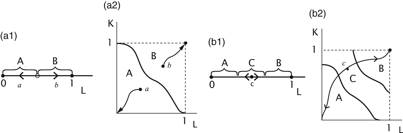
Figure 1 illustrates the relation between the models with one and with two state variables, and the distinction between the two interpretations of ‘more likely’. In the model with one state variable (L), illustrated by panels (a1) and (b1), the state space is [0, 1]; there are two steady states, L=0 and L=1 where, respectively, all labor is in Agriculture or in Manufacturing. In the model with two state variables, (L, K), illustrated by panels (a2) and (b2), the state space is the unit square. Here there are two stable steady states, (0, 0) and (1, 1). In the first, all labor is in Agriculture and the pollution stock is zero, so agricultural productivity is high. In the second, all labor is in Manufacturing and pollution is at its maximum level, equal to 1, causing agricultural productivity to be low.
Phase space for different models. (a1) one-state, unique equilibrium; (a2) two-state, unique equilibrium; (b1) one-state, multiple equilibria; (b2) two-state, multiple equilibria.

In panels (a1) and (a2), the basins of attraction for the steady states, in both the one-state and the two-state models, are the sets A and B. These sets are intervals in the one-state model and regions in the two-state model. The sets A and B have no intersection except for the boundary, which is of measure 0. A typical interior point a ∈ A (or b ∈ B) has a unique trajectory to the steady state where all labor is in Agriculture (respectively, Manufacturing). Panels (a1) and (a2) illustrate the situation where the equilibrium is unique and there is hysteresis: the steady state depends on the initial condition.
In contrast, in panels (b1) and (b2) the state space consists of three sets, A,B and C. The basin of attraction for the steady state with all labor in Agriculture is  $A \cup C$ and the basin of attraction for the steady state with all labor in Manufacturing is
 $B \cup C$. The intersection of these two sets, C, is the ROM. From point c ∈ C there are two trajectories, approaching different steady states. The equilibrium is not unique in the models represented by panels (b1) and (b2), because there is a set of initial conditions, with positive measure, for which there are multiple equilibrium trajectories.
According to Interpretation 1, a decrease in friction makes multiplicity more likely if it increases the measure of the set of parameters for which panels (b1) or (b2) rather than panels (a1) or (a2) describes the dynamics. According to Interpretation 2, the decrease in friction makes multiplicity more likely if it increases the measure of the ROM, C.
The chief result from our two-dimensional model is that there is a non-monotonic relation between the measure of the ROM and friction in the adjustment for labor. Thus, according to Interpretation 2, a decrease in labor adjustment costs may make multiplicity either more or less likely. A decrease in labor adjustment costs does, however, increase the set of other parameter values for which the ROM is positive. Thus, according to Interpretation I, lower adjustment costs make multiplicity more likely, just as in the standard one-state models. But according to Interpretation 2, lower adjustment costs might make multiplicity either more or less likely. Taken together, the two results imply that if labor adjustment costs are extremely small, the measure of the ROM is positive for a wide range of parameter values, but the measure is always extremely small. Multiplicity in this case is possible, but it occurs only for a small set of initial conditions and in that sense is not likely.
For the type of model we consider, this non-monotonicity requires the second state variable, e.g. a stock pollutant instead of a flow pollutant. However, the non-monotonicity survives even if the stock pollutant decays very quickly. In that case, the amount of damage-creating pollution remaining over a small interval of time closely tracks the emissions flow during that interval – because emissions flows over previous periods have already largely dissipated. In this respect, the two-state model with rapidly decaying stock appears to approximate a one-state model with a flow pollutant. Nevertheless, the non-monotonicty does not arise under a flow pollutant. Thus, two models that appear similar might lead to different types of results.
Even if the pollution stock decays rapidly (causing the stock to closely track the pollution flow), it remains possible for the labor allocation to change still more quickly. Rapid adjustment of labor requires that migration costs be small. When the speed of adjustment in the labor market is fast relative to the speed of adjustment of the pollution stock, a worker can move between sectors quickly enough to insure that she remains in the high wage sector ‘most of the time’. In this case, for most initial conditions, the worker's migration decision is not sensitive to her beliefs about what other workers will do. Multiplicity is possible, but the ROM is small.
We use a deterministic model and assume that agents have rational point expectations: they correctly anticipate the evolution of the economy. If agents were myopic, there would be no role for expectations to influence behavior. There might nevertheless be multiple stable steady states, each with its basin of attraction. In this case, there would be hysteresis, but not multiplicity of equilibria (as we use that term).
1.2 Literature review
Previous literature, excepting Krugman (Reference Krugman1991), Fukao and Benabou (Reference Fukao and Benabou1993) and Karp and Paul (Reference Karp and Paul2007), neglects the relation between parameters of the model and the measure of the ROM, and concentrates on the relation between parameter values and the existence of a ROM with positive measure. There are two likely reasons for this emphasis. First, although it is sometimes straightforward to determine conditions under which the ROM has positive measure, the comparative statics of this measure are complicated. Second, intuition (supported by Krugman's model) may have encouraged the idea that the two senses in which a parameter change can make multiplicity ‘more likely’ are essentially the same.
Multiplicity of equilibria arises when there are increasing returns to scale, or some other feature that makes the economy non-convex. Greater convexity of adjustment costs (more generally, increased friction) appears to counteract the effect of cross-sectoral pollution or increasing returns to scale. Therefore, a natural conjecture is that more convex adjustment costs make multiplicity less likely. Karp and Paul (Reference Karp and Paul2007) use numerical methods to show that this conjecture is not true in general in a two-state version of Krugman (Reference Krugman1991). Here we use a simpler framework and obtain analytic results, thereby improving our intuition for this type of model.
There is little empirical evidence regarding the type of multiplicity we described above. Davis and Weinstein (Reference Davis and Weinstein2002, Reference Davis and Weinstein2004) find that Japanese data is consistent with increasing returns to scale, but that the data is inconsistent with the existence of multiple stable steady states – a necessary condition for multiplicity of equilibria in this setting. Moro (Reference Moro2003) estimates a multiple equilibrium model of wage inequality; Brock and Durlauf (Reference Brock and Durlauf2001, Reference Brock and Durlauf2002) discuss the estimation of discrete choice models with social interactions, a situation that can lead to multiple equilibria.
There is a different type of multiplicity, often referred to as ‘indeterminacy’, that occurs when there exists a continuum of equilibrium trajectories to a single steady state. Indeterminacy is an important topic in macro-economics, where the role of costs of adjustment (friction) is significant. Benhabib and Farmer (Reference Benhabib, Farmer, Taylor and Woodford1999) review this literature; recent contributions include Cooper and Haltiwanger (Reference Cooper and Haltiwanger1996), Cooper and Johri (Reference Cooper and Johri1997), Wen (Reference Wen1998a,Reference Wenb), Benhabib et al. (Reference Benhabib, Meng and Nishimura2000), Nishimura and Shimonura (Reference Nishimura and Shimonura2002) and Lubik and Schorfheide (Reference Lubik and Schorfheide2004). A recurring question concerns the specification for which plausible estimates of adjustment costs and returns to scale are consistent with indeterminacy. In these models, lower costs of adjustment (less friction for the mobile factor) mean that indeterminacy is more likely, using Interpretation 1. Since the analysis of these models (typically) examines behavior in the neighborhood of the steady state, no attention is paid to Interpretation 2.
Recent theoretical papers show that changing an assumption of migration models may eliminate the multiplicity of equilibria. Frankel and Pauzner (Reference Frankel and Pauzner2000) show that multiplicity disappears in a variation of Matsuyama's model where the wage differential is subject to Brownian motion and there exist ‘dominance regions’. In another variation of this model, Herrendorf et al. (Reference Herrendorf, Valentinyi and Waldman2000) show that there is a unique equilibrium if agents are sufficiently heterogeneous. We provide another explanation that might either increase or diminish the importance of coordination problems.
2. The model
The discrete time model makes it easy to obtain the comparative static results in section 3. To introduce our model and also to establish the connection between our discrete time formulation and previous literature, we begin with a one-state, two-period formulation (section 2.1). This model reproduces the major insights from Krugman (Reference Krugman1991) who considers increasing returns to scale that are external to firms, whereas we focus on cross-sectoral pollution, where both sectors have constant returns to scale. This difference changes the interpretation of the one-state model but not the nature of the results.
Our contribution uses a two-state, three-period model where all migration occurs during the first two periods (section 2.2). We use the two-state, three-period model in section 3 to show analytically that an increase in intersectoral labor mobility (a decrease in friction) can reduce the set of initial conditions from which there emanate multiple equilibrium trajectories. That is, an increase in mobility can decrease the measure of the ROM, and in this respect make multiplicity less likely.
2.1 The two-period, one-state model
This section obtains the insights from Krugman's continuous time formulation using a two-period model. The initial stock of labor in Manufacturing is 0 ≤ L ≤ 1 and the measure of entrants into Manufacturing is u, so the amount of labor in Manufacturing in the next period is L+u. Workers who move incur a cost of migration in the current period and (possibly) obtain a higher wage in the next. The discount factor is β. The manufacturing wage is fixed at α M. Pollution arising from the manufacturing sector in the second period equals L+u. Average and marginal productivity (and thus the wage) in Agriculture in this period equals α A − b(L + u); each unit of pollution lowers the wage in Agriculture by b units. This one-state variable model describes a flow pollutant. The Manufacturing-Agriculture wage differential in the second period therefore equals a + b(L + u), with a ≡ α M − α A. We assume that a<0 and a+b>0: if all workers are in the same sector, that is the high-wage sector.
The social cost of migration is u 2/2γ, with γ > 0. Migration services are competitively supplied, so the price of migration (the amount that a migrant pays in order to switch sectors) is |u|/γ. A higher value of γ means that adjustment costs are lower: there is less friction. An agent who decides to migrate pays the migration cost in the current period, in order to be in a different sector at the next period.
The present value of the benefit minus the cost of migrating to Manufacture (u>0) or to Agriculture (u<0) equals the present value of the wage differential minus the cost of migration:
 $$n(L,u)\equiv \displaystyle{{1}\over{\gamma}} ( \beta \gamma ( a+b ( L+u) ) -u )$$
For bγβ < 1, the net benefit of migration decreases with the number of other agents migrating. In this case, actions are strategic substitutes and the equilibrium is unique. Agents play a coordination game (i.e. actions are strategic complements), and there are multiple equilibria, if and only if bγβ > 1, as we hereafter assume.
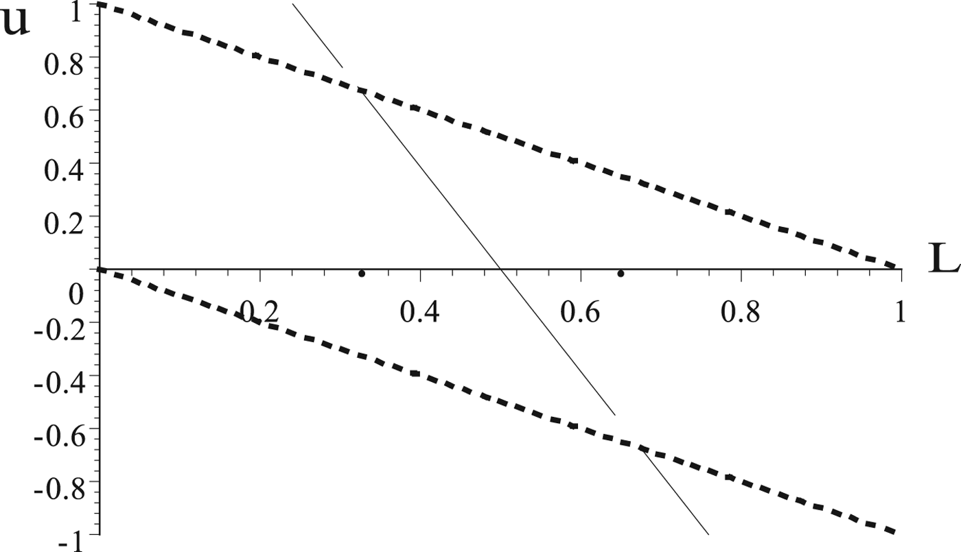
Figure 2 graphs the migration constraints 0 ≤ L + u ≤ 1 (the dotted lines) and the solution to n=0 for bγβ > 1 (the solid line). The L coordinates of the points of intersection between the graph of n=0 and the migration constraints (the heavy dots in figure 2) define the interval [1 − (a + b)βγ, − βaγ]. This interval corresponds to the interval C in figure 1, panel (b1). The ROM consists of the intersection of this interval and the set of feasible initial conditions, [0, 1]. For an initial condition (a value of L) in the ROM, the value of u that satisfies n(L, u) = 0 (i.e., a point on the solid line) is an unstable equilibrium.Footnote 1 At initial conditions inside the ROM there are two stable equilibria: all labor moves to Manufacturing or to Agriculture. For example, at u=1−L for L ∈ ROM, the benefit of moving to Manufacturing exceeds the cost (n(L, 1 − L) > 0) so it is a stable equilibrium for all labor to move to Manufacturing. The length of the ROM is
 $$\hbox{Length of ROM} = \max \{0,\min \{ 1,-\beta a\gamma \} )-\max \{ 0,1-(a+b)\beta \gamma \} \}.$$
For initial conditions to the left of the ROM, the unique equilibrium sends all labor to Agriculture. For initial conditions to the right of the ROM, the unique equilibrium sends all labor to Manufacturing.
The ROM in a one-period model with  $\beta \gamma G>1$. The heavy dots, given by the L coordinates of the solid and the dotted lines, show the boundary of the ROM.

The existence of multiplicity requires a combination of patience, a large externality, and low adjustment costs (large values of β, b, γ), just as in Krugman (Reference Krugman1991). An increase in any of these factors increases the length of the ROM when this is positive and less than 1. Thus, lower adjustment cost makes multiplicity ‘ more likely’ in both senses described in the Introduction.
For this model we do not need any assumptions about the measure used to assess the likelihood of multiplicity; that is, the statement that multiplicity becomes more likely is independent of the priors on the initial condition and on b and β. For example, an increase in γ can cause initial conditions to enter the ROM but never cause initial conditions to leave the ROM. Here, there is no loss in generality in using the length of the ROM to measure the likelihood of multiplicity. This measure corresponds to a uniform prior over initial conditions.
2.2 The three-period, two-state model
This section introduces the model that we use to establish the non-monotonicity of the ROM with respect to labor adjustment costs. Current migration affects the labor allocation in the next period, and current pollution affects the pollution stock in the next period. The period index is t ∈ {0, 1, 2}. The predetermined stock of pollution in period t equals K t and the flow of pollution in period t is GL t, with G>0. Each unit of labor in Manufacturing in the current period adds G units to the next-period pollution stock. The stock of pollution in t+1 is
 $$K_{t+1}=K_{t}+G ( L_{t}-K_{t}) \Rightarrow K_{t+1}-K_{t} = G (L_{t}-K_{t}).$$
Each unit of this stock reduces productivity in Agriculture by b units. The pollution stock at t is predetermined, so the Agriculture wage at t is α A − bK t. The Manufacturing wage is fixed at α M, so the Manufacturing-Agriculture wage differential is α A − α M − bK t = a − bK t.
In order to focus on our research question, we hereafter set a=0.5 and b = 1, so the wage differential is 0.5 − K t. With this choice of parameters, the wage differential equals 0 at K=0.5. Using equation (3), the pollution stock is constant at K=0.5 only for L=0.5. Thus, K = L = 0.5 is the only interior steady state for this linear model. Just as in the one-state model, this interior equilibrium is unstable. To further simplify notation, we define the state variables as deviations from these values: l t ≡ L t − 0.5 and k t ≡ K t − 0.5. By construction, k t equals the Manufacturing-Agricultural wage differential in period t. The state space for the model is the square
 $${-}0.5\leq l_{t}\leq 0.5, \ -0.5\leq k_{t}\leq 0.5,$$
and the equation of motion for the transformed pollution stock is
 $$k_{t+1}=k_{t} + G ( l_{t}-k_{t}).$$
Migration decisions are made at t=0 and at t=1. Agents base their migration decisions on their beliefs about wages in periods t=1 and t=2 and on migration costs in periods t=0 and t=1. Denote the amount of migration to Manufacturing in period 0 as u (as in the one-period model) and the amount of migration to Manufacturing in period 1 as v. Negative values mean that migration is into Agriculture. The social cost of migration is quadratic in migration, and the price that a migrant pays is | u|/γ in period 0 and | v|/γ in period 1. In the initial period, (t=0), the state variables L 0, K 0 are given.
We adopt the following parameter restriction:
 $$0 \lt G\leq 1.$$
This restriction and equation (3) imply that the next-period pollution stock is a convex combination of the current pollution stock and the current flow. Because our objective is to demonstrate and explain a counter-intuitive result, it is sufficient to show that the result holds for reasonable – not for all – parameterizations.Footnote 2 Section 3.2 notes that inequality (6) has a physical interpretation. If we think of the discrete time model as an approximation to a continuous time model, the value G=1 corresponds to the fastest possible speed of adjustment of the pollution stock. The special case G=1 also leads to particularly sharp analytic results.
3. Results
We first state our principal result. The next section contrasts the comparative statics of the ROM, with respect to γ, in the one-state and the two-state models. A final section offers a different perspective, sketching a continuous time model.
Our principal results use the following definitions:
 $$\eqalign{X(k_{0}) & = -\displaystyle{{\phi}\over{\chi}}k_{0} -0.5 \displaystyle{{\gamma \beta ^{2}G-1}\over{\chi}} \cr Y(k_{0}) &= -\displaystyle{{\phi}\over{\chi}}k_{0}+0.5 \displaystyle{{\gamma \beta ^{2}G-1}\over{\chi}}},$$
where
 $$\eqalign{\chi & =\gamma \beta G ( \gamma G\beta +3+\beta -\beta G-G) +1 \cr \phi & =\gamma \beta ( \gamma \beta G+2.0-1.0\gamma \beta G^{2}-3.0G+G^{2}-2.0\beta G+ \beta +\beta G^{2})}.$$
The following Proposition summarizes our main results; the appendix contains the proof.
Proposition 1 Suppose that inequality (6) holds in our three-period model.
(i) β 2Gγ > 1 is necessary and sufficient for the ROM to have positive measure. Thus, an increase in γ (i.e., a decrease in friction) increases the range of other parameter values ( β and G ) for which the ROM has positive measure.
(ii) The ROM is defined by the following set:
 $${\rm ROM} = \{(k,l):-.5\leq k\leq .5\cap -.5\leq l\leq .5\cap Y(k)\leq l\leq X(k)\}.$$
(iii) For β 2Gγ > 1, the area of the ROM is non-monotonic in γ.

The condition for the ROM to have positive measure, β 2Gγ > 1, is essentially the same as for the one-state variable model (with G playing a role analogous to b) except that here the condition involves β 2 rather than β. This difference arises because in the two-state variable model migration in period t affects the wage differential in period t+2 rather than in period t+1 (as was the case in the two-period model). The lag occurs because here the pollution stock mediates the effect of a change in labor allocation. In the one-state variable model, which describes a flow pollutant, the change in labor allocation has an immediate effect on the wage differential.
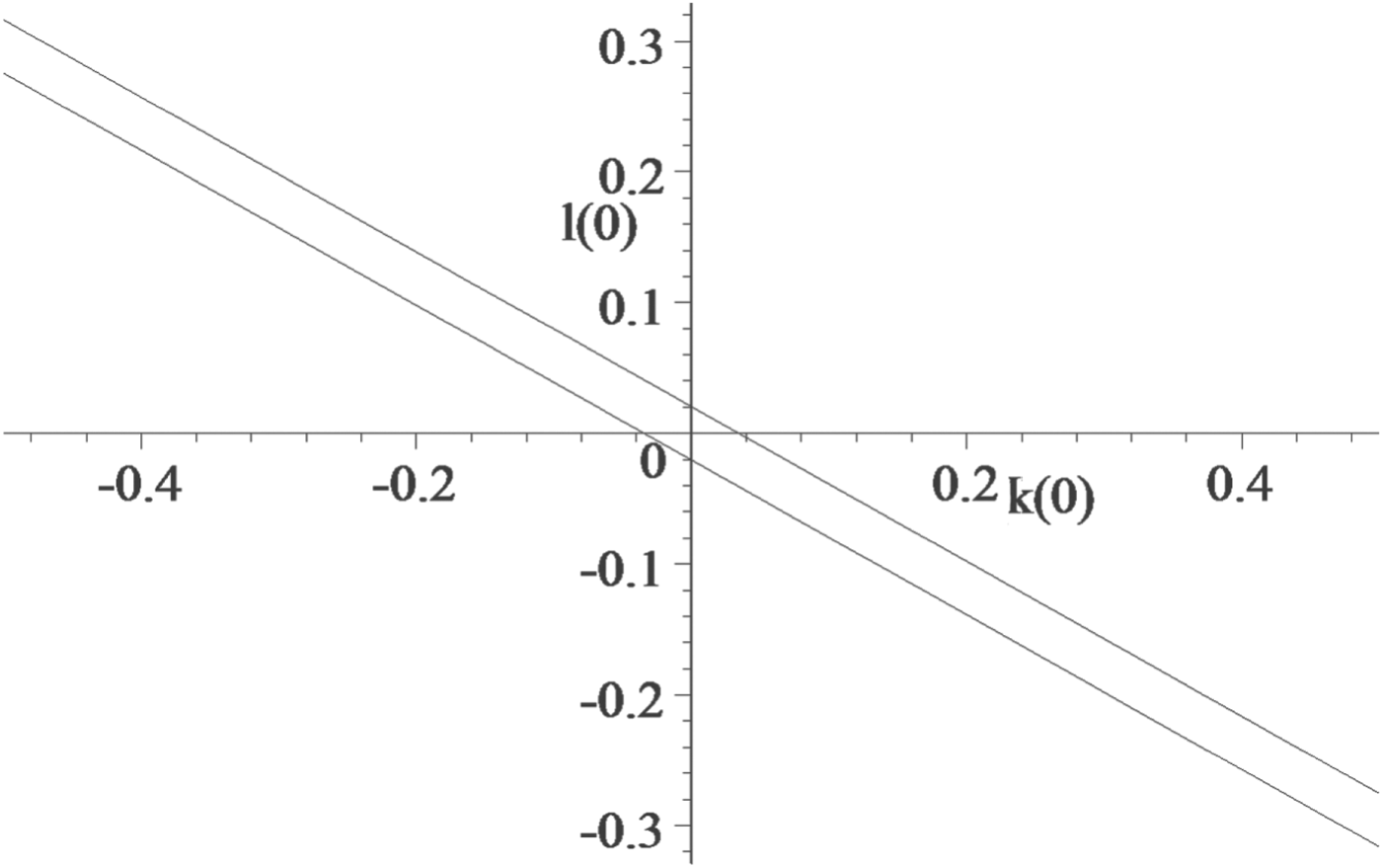
Figure 3 shows an example of the ROM. (Compare to figure 1, panel (b2).) The lower line is the graph of X and the upper line is the graph of Y, defined in equation (7). The area between these two lines is the ROM. Restriction (6) and β 2Gγ > 1 imply that χ > 0. This fact, equation (7), and the assumption that γβ 2G > 1 imply that X<Y. For any k 0, the vertical distance between Y and X is
 $$M\equiv Y-X=\displaystyle{{\gamma \beta ^{2}G-1}\over{\chi }}>0.$$
The ROM (area between lines) for β = 0.8,G = 0.5,γ = 2.5.

In general, we do not have a simple closed form expression for the area of the ROM. However, if Y(0.5) < −0.5 or X(0.5) > −0.5, then the ROM does not include the NW or SE corners of state space, and the ROM is a parallelogram. If X(0.5) > −0.5, the area of the ROM is simply M.Footnote 3
Interpretation 2 states that a parameter change increases the measure of the ROM. In general, checking this condition requires that we define the ‘measure’, i.e. a probability distribution for the set of initial conditions. For example, if the initial conditions are uniformly distributed over the unit square (the state space), then an increase in the area of the ROM unambiguously raises the likelihood that an arbitrarily chosen initial condition lies in the ROM. However, for a non-uniform distribution, an increase in the area of the ROM does not, in general, imply that it is ‘more likely’ that an initial condition lies in the ROM. For general parameter values, a change in γ causes the ROM to rotate as its area changes. Therefore, for two values of γ, γ 1 ≠ γ 2 the inequality area(ROM(γ 1)) > area(ROM(γ 2) does not imply that ROM(γ 2) ⊂ ROM(γ 1). Consequently, unless the distribution of initial conditions is uniform over state space, the fact that area(ROM(γ 1)) > area(ROM(γ 2) does not necessarily mean that multiplicity is more likely under γ 1 than under γ 2.
In contrast, for the special case G=1, equation (5) implies that the wage differential in the next period does not depend on the current wage differential (the current value of k). When G=1 the ROM is flat; its boundaries are independent of k 0. For G=1, the magnitude of γ affects only the vertical distance between the two lines in figure 3. In this case, area(ROM(γ 1)) > area(ROM(γ 2) does imply that Rom(γ 2) ⊂ Rom(γ 1). Thus, for G=1, a larger area of the ROM means that multiplicity is ‘more likely’, regardless of the distribution of the initial condition.
3.1 Comparison of one-state and two-state models
We noted that the presence of a second state variable (the stock of pollution) changes the relation between the amount of friction in labor adjustment and the likelihood of multiplicity of equilibria, as captured by the measure of the ROM. There are two reasons why the case G=1 is particularly useful for illustrating this difference. First, as noted above, in this situation there is no loss in generality in using a uniform prior for initial conditions. Second, the case G=1 is of special interest because it leads to a model that appears to approximate the one-state variable model. Recall that G=1 corresponds to complete adjustment of the pollution stock, following changes in L, within a single period. That is, when G=1 the stock of pollution adjusts very rapidly – precisely the situation where we might expect that a one-dimensional model provides a good approximation to the two-dimensional model.
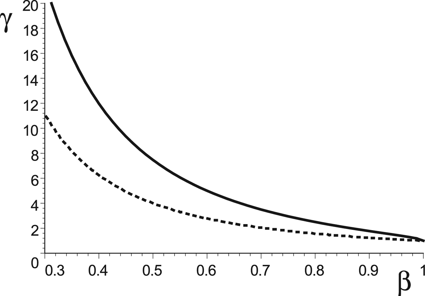
When G=1 the area of the ROM is max{0, M}, with M = γβ 2 − 1/γ 2β 2 − 1. Thus, γ > β −2 is necessary and sufficient for the ROM to have positive measure when G=1. For β = 1, M = 1/γ + 1, which is strictly decreasing in γ. For β < 1, M is first increasing in γ (in the neighborhood β −2) and then decreasing. The measure reaches its maximum at  $\gamma ^{m}\equiv {1}/{2\beta ^{2}} (2+2\sqrt {1-\beta ^{2}}) $ and thereafter decreases. The maximum point γ m converges to β −2 as β → 1.
Figure 4 shows the graph of γ m (the solid curve) and of β −2 (the dotted curve). For combinations of (β, γ) below the dotted curve, the measure of the ROM is 0; for a point between the two curves, the measure of the ROM is increasing in γ, holding β fixed; and for points above the solid curve, the measure is decreasing in γ, holding β fixed.
For G=1, measure of ROM is 0 below the dotted curve, increasing in γ between curves, and decreasing in γ above solid curve.

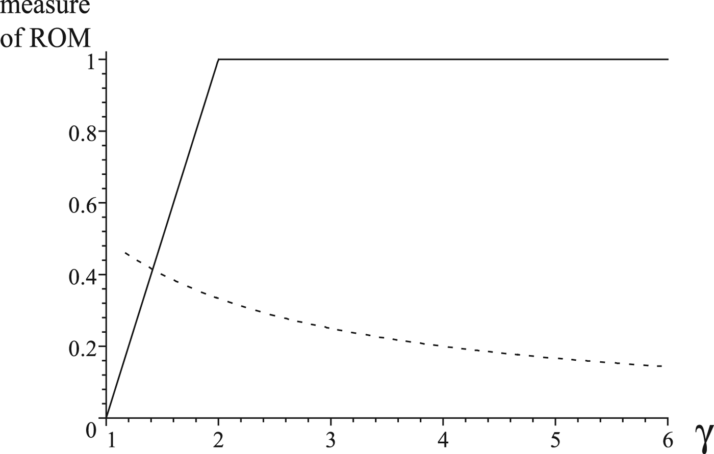
In presenting the model with two state variables, we set b=1 and a=−0.5. Therefore, to compare the two models we need to use these values in the model with one state variable. Here we also set β = 1, so that the necessary and sufficient condition for a positive measure of the ROM is γ > 1 in both models. With these restrictions, figure 5 graphs the measure of the ROM in the two models, for γ > 1. This figure uses equations (2) and (8). The figure shows that the friction parameter γ has the opposite effect on the measure of the ROM in the two models.
Meausure of ROM, with β = G = b = 1. The solid curve shows that for the model with one state variable, the measure increases with γ. The dotted curve shows that for the model with two state variables, the measure decreases with γ.

3.2 A different perspective
Here we sketch a continuous time model to make three points. First, it provides a physical interpretation of restriction (6). Second, it shows that our discrete time model can be viewed as an approximation of a continuous time model. Third, the idea of two state variables adjusting at different speeds is transparent in the continuous time setting, but not in the discrete time setting. The online appendix describes a more general model.
The continuous time analog of equation (3) is
 $$\dot{K}=g ( L_{t}-K_{t}).$$
If we hold L t in equation (9) constant for one unit of time and solve that equation, to rewrite it in the same form as equation (3), we see that the relation between the two parameters is G = 1 − e −g. Because g ≤ ∞, the restriction G ≤ 1 is reasonable. Of course G>0 because the pollution flow affects the stock.
Define a ‘provisional’ steady state of pollution as the steady state corresponding to a fixed value of labor allocation. For example, consider two economies. The first has been largely rural, with only 5 per cent of its labor force in Manufacturing (L=0.05), and the second has been industrialized, with 95 per cent of labor in the Manufacturing sector (L=0.95). If the two economies have been at their respective stages for a long period of time, then in both economies the respective pollution stocks will be close to their ‘provisional’ steady states: K=0.05 for the first economy and K=0.95 for the second. These are the values of K that solve  $\dot {K} =0$ in equation (9). The relatively low level of manufacturing in the first economy corresponds to a relatively cleaner environment.
In the continuous time setting, adjustment to a provisional steady state can be made arbitrarily rapid, by increasing the speed of adjustment parameter g in equation (9). As g → ∞, the pollution stock adjusts instantaneously. For large g, the pollution stock never deviates far from the pollution flow. Therefore, for large g a flow pollutant model approximates a stock pollutant pollutant model. In contrast, in the discrete time setting with our timing convention, adjustment of pollution to a provisional steady state takes at least one period, i.e. it always occurs with a lag. The two-state discrete time model cannot exactly reproduce the one-state model.
Define u as the flow of labor into Manufacturing (for u>0) or into Agriculture (for u<0), so dL/dt = u. The flow cost of migration is  ${u_{t}^{2}}/{2\gamma }$, so a migrant at time t pays the migration cost |u t|/γ. As in Krugman's one-state model, γ is inversely related to friction; γ is a speed-of-adjustment parameter for labor. When g and γ differ by orders of magnitude, the time scales over which the two state variables change are different: there are ‘slow-fast dynamics’. Equation (9) can be rewritten as
 $$\displaystyle{{\dot{K}}\over{g}}=L_{t}-K_{t}.$$
In the limit, as g → ∞, equation (10) implies that K t = L t, which implies that the Manufacturing-Agricultural wage differential in period t is L t − 0.5. This formula for the wage differential is the same as in Krugman's setting, using a=−0.5 and b=1. (We adopt these two parameter restrictions only to simplify the exposition.) More generally, when g is large (for fixed γ), K adjusts rapidly, relative to the speed of adjustment of L. Here, the pollution stock closely tracks L: K ≈ L for g large.
Thus, it would appear that the one-state model should provide a good approximation to the two-state model when the pollution stock adjusts rapidly. However, the two models have different implications concerning Interpretation 2. Provided that g < ∞, by making γ large migration becomes cheap enough that a worker can be sure of being in the high wage sector ‘most of the time’, regardless of other workers' decisions. In this case, a worker bases her migration decision primarily on the state variables, not on her beliefs about what other workers will do. Multiplicity is still possible, but it occurs for a small set of initial conditions: it is unlikely.
When g is finite, current migration affects the second time-derivative of the wage differential,
 $$\displaystyle{{d^{2} (K-0.5)}\over{dt^{2}}} = g (u-g(L-K)).$$
In contrast, in Krugman's model (g = ∞), current migration affects the first time-derivative of the wage differential. The presence of the second state variable mediates migration's effect on the wage differential. In a discrete time setting, we saw that the presence of the second state variable causes migration to affect the wage differential with a lag.
4. Conclusion and discussion
Many dynamic models can be viewed as extensions of static models, obtained by introducing a payoff-relevant state variable that adjusts over time. There are usually many ways of making a model dynamic. If we think that the friction in the adjustment of the mobile factor is the single most important source of dynamics, it is essential to include the labor allocation as a state variable. The additional complexity that comes from including a second state variable is a powerful argument in favor of the one-state model.
In addition, we may think that the one-state model is adequate. For example, we might agree that the cross-sectoral externality is not literally associated with the pollution flow, and that instead it is associated with a pollution stock. However, if the pollution stock tracks the flow very closely, it might appear that there would be little loss of economic insight in replacing the pollution stock with the flow, thereby using a one-state model. In a standard optimal control setting (i.e., a game against nature), when the speed of adjustment of different state variables differs by orders of magnitude, a higher dimensional problem can often be well-approximated using a lower dimensional state space. Where technology is convex, a competitive equilibrium can be obtained by solving a planner's optimization problem.
However, in nonconvex settings, an equilibrium problem involving agents with rational expectations can give rise to multiple equilibria. In this situation, it is typically not possible to obtain the equilibrium by solving a planner's problem. Here, an apparently innocuous reduced-dimensional ‘approximation’ of a higher dimensional state space might change important features of the problem. We used a simple model with two state variables to illustrate and explain this possibility.
When we ask how an increase in labor adjustment costs affects the likelihood of multiplicity, we might have in mind two different relations. Friction affects the measure of the set of (other) parameter values under which multiplicity is a possibility, and it affects the measure of the set of initial conditions for which multiplicity actually occurs. In Krugman's model and in our two-period simplification, the answer to the comparative statics question is the same, regardless of which of these two interpretations we have in mind. The theoretical and empirical literature on indeterminacy emphasizes the first interpretation. There is little discussion in the literature involving the second interpretation, which is arguably as important as the first.
We showed that when the labor allocation affects the wage differential with a lag, either because of an environmental stock externality or due to a stock of knowledge arising from learning-by-doing, then the answer to the comparative statics question may differ, depending on which interpretation one adopts. Under the first interpretation, a decrease in friction always makes multiplicity more likely in our model, just as in the one-state setting. Under the second interpretation, the relation is non-monotonic, unlike in the one-state setting.
When it is harder for an agent to take an action, such as moving to a new sector, it seems that there would be fewer initial conditions under which her decision would depend on beliefs about what other agents will do. This conclusion is (by now) so well-established that it seems obvious. However, when the current wage differential is sluggish, as occurs in our two-state model, the relation is reversed for low cost of labor adjustment. With low adjustment costs, for most initial states the agent's equilibrium migration decision does not depend on beliefs about what others will do; whatever their actions, it is cheap for an agent to move in future periods in order to remain in the high wage sector. That is, for most initial conditions, agents have a dominant strategy when adjustment costs are low.
This theoretical point shows the danger of drawing conclusions about the importance of multiplicity based on estimates of structural parameters of the model (i.e., based on Interpretation 1). Parameter estimates might suggest, for example, that there are significant cross-sectoral negative externalities or within-sectoral increasing returns to scale (or some other source of non-convexity); that factor adjustment costs are very low; and that a one-state variable model apparently provides a good approximation to the economy (because other state variables adjust rapidly). The conventional wisdom is that in these circumstances the ROM is likely to have positive measure. Our results agree with this conclusion, but also suggest that the measure of the ROM is likely to be very small, and therefore the economy is unlikely to have multiple equilibria.
An economy that has multiple steady states but a unique equilibrium might evolve in very different ways, depending on the initial condition. For example, an exogenous change in pollution control technology or environmental policy can change incentives about where to invest. Those kinds of exogenous changes can alter an interior steady state, leading to standard comparative statics results. If the changes in pollution control or policy are small, we expect the change in the steady state to also be small. However, those exogenous changes might shift the basins of attraction. If the shift causes a predetermined state variable to now reside in a different basin of attraction, the small exogenous change can cause the system to approach a different steady state. In that case, the exogenous change causes a large change in the equilibrium trajectory, even though each of the steady states has changed by a small amount.
Matters are even more complicated if there are multiple steady states and also multiple equilibria, i.e. if the ROM has positive measure. Here, where the outcome depends on agents' beliefs as well as economic fundamentals, the standard application of comparative statics might tell us very little. We would have to know how the exogenous change alters agents' beliefs.
Supplementary material
The supplementary material for this article can be found at https://doi.org/10.1017/S1355770X19000147.
Acknowledgments
We thank Tasos Xepapadeas and two anonymous referees for comments on an earlier draft. The usual disclaimer applies.
Appendix A: Proof of Proposition 1
We construct the equilibrium by working backwards, beginning with the agents' problem in period 1, the last period during which they can migrate.
Using equation (5) and l 1 = l 0 + u, we write the present value at t=1 of being in Manufacturing in period 2, as
 $$\beta k_{2}\,=\,\beta (k_{1}+G(l_{1}-k_{1})) \,=\, \beta (G(2-G)l_{0}+(G-1)^{2}k_{0}+Gu)\equiv f(u;k_{0},l_{0}).$$
Our timing conventions imply that this value is predetermined at period 1. The equilibrium for the subgame beginning in period 1 is therefore unique. Agents are indifferent between migrating and staying in their current sector if and only if βk 2 = v/γ, i.e. if v = γf(u;l 0, k 0). The speed of adjustment parameter affects the magnitude but not the sign of the quantity γf( · ), and f( · ) is increasing in u for all G>0.
Taking into account the labor supply constraint, the equilibrium value of v is
 $$v(u)=\left\{\matrix{0.5-l_{0}-u & {\rm if} & \gamma f>0.5-l_{0}-u \cr \gamma f & {\rm if} & -0.5-l_{0}-u\leq \gamma f\leq 0.5-l_{0}-u \cr -0.5-l_{0}-u & {\rm if} & \gamma f<-0.5-l_{0}-u}\right\}.$$
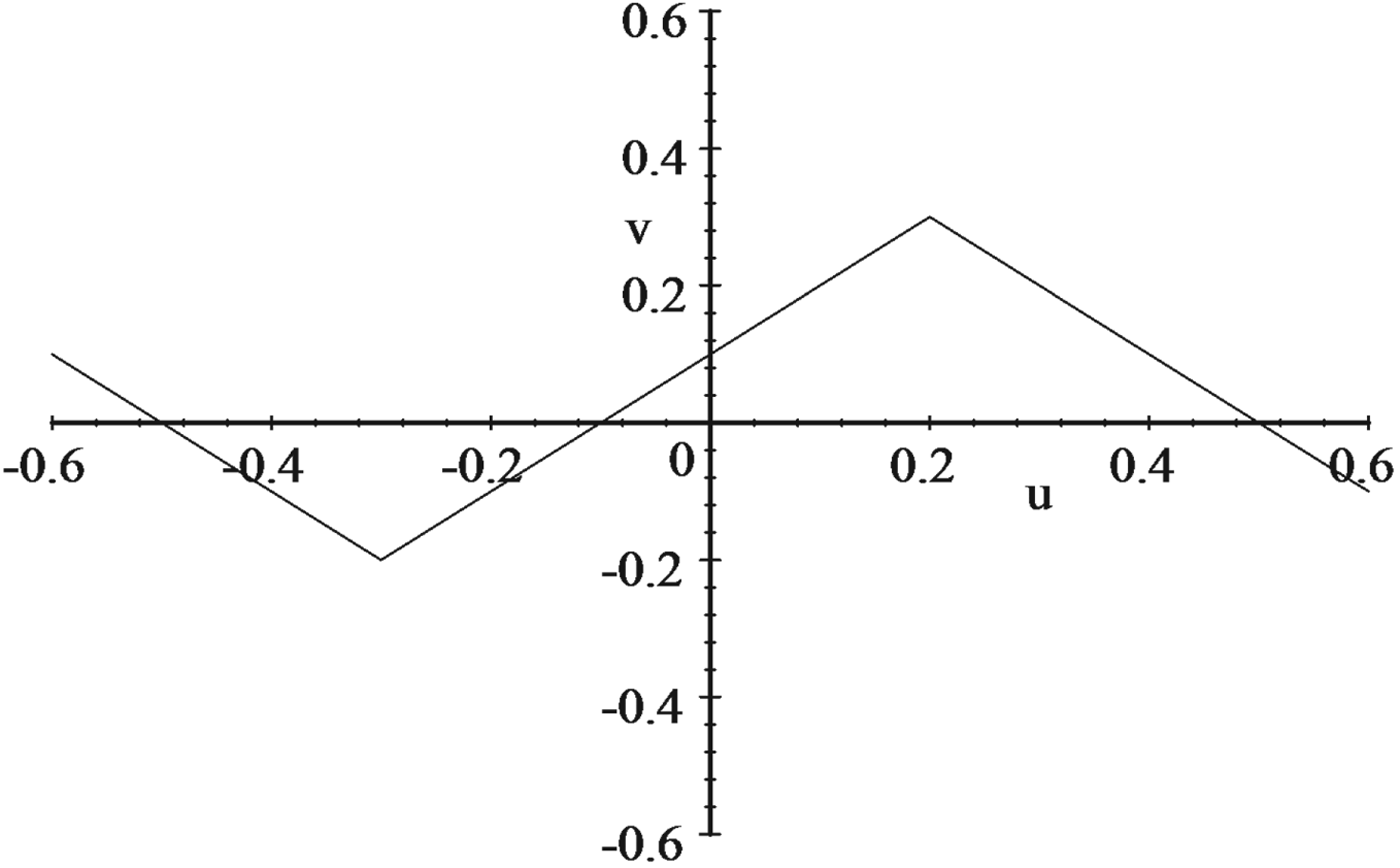
Figure A6 shows an example of the graph of v(u), given particular values l 0 = 0 and k 0 > 0.
Equilibrium second period migration (v) as a function of first period migration (u) for β = 0.8, γ = 2.5, G=0.5, l 0 = 0 and k 0 = 0.2.

The u coordinate of the left and the right kink in this graph are, respectively
 $$\matrix{{\rm left kink}{\rm : \ } & p\equiv \rho (l_{0},k_{0})-\displaystyle{{0.5}\over{1+\gamma \beta G}} \cr {\rm right kink}{\rm : \ } & q\equiv \rho (l_{0},k_{0})+\displaystyle{{0.5}\over{ 1+\gamma \beta G}},}$$
using the definition
 $$\rho (l_{0},e_{0})\equiv \displaystyle{{1}\over{1+\gamma \beta G}}(\gamma \beta G(G-2)-1)l_{0}-\gamma \beta (G-1)^{2}k_{0}).$$
For all l 0 and k 0, it is always the case that p<q. Inequality (6) implies that ρ is a decreasing function of l 0, so p and q are decreasing functions of l 0 – a fact that we use below.
Using these definitions and equation (A1) implies
 $$\displaystyle{{dv(u)}\over{du}} = \left\{\matrix{-1 & {\rm if} & u>q \cr \beta G\gamma & {\rm if} & p<u<q \cr -1 & {\rm if} & u<p}\right\}.$$
Thus, an increase in u increases the equilibrium v, provided that v is interior. In contrast, an increase in u decreases the equilibrium v when this variable is on the boundary of the labor supply constraint, as figure A6 illustrates.
In period 1 an agent is either indifferent between migrating and staying in her current sector (at an interior equilibrium) or she strictly prefers to migrate (at a boundary equilibrium). Agents with rational expectations understand this fact in period 0. Therefore, the benefit of migrating to Manufacturing in period 0 is the present value of the wage differential in period 1 (βk 1), plus the present value of migration costs in period 1 (βv(u)/γ).Footnote 4 The present value of migrating to Manufacturing in period 0 is therefore
 $$\beta \left( k_{1}+\displaystyle{{v (u)}\over{\gamma}}\right) \,=\,\beta \left( (1-G)k_{0}+Gl_{0}+\displaystyle{{v (u)}\over{\gamma}}\right).$$
If the value of this expression is negative, its absolute value is the value of migrating to Agriculture. For u > 0, the cost of moving to Manufacturing in period 0 is u/γ; for u<0, the cost of moving to Agriculture is − u/γ.
Define the difference between benefits and costs of moving to Manufacturing in the first period as
 $$h(u;l_{0},k_{0})\equiv \beta \left( (1-G)k_{0}+Gl_{0}+\displaystyle{{v(u)}\over{\gamma}} \right) -\displaystyle{{u}\over{\gamma}}.$$
(Again, if h<0, then − h is the value of moving to Agriculture.) Using equation (A2), we have
 $$\displaystyle{{dh}\over{du}}=\left\{\matrix{\displaystyle{{-\beta -1}\over{\gamma}} & {\rm if} & u>q \cr \displaystyle{{\beta ^{2}G\gamma -1}\over{\gamma}} & {\rm if} & p<u<q \cr \displaystyle{{-\beta -1}\over{\gamma}} & {\rm if} & u<p}\right\}.$$
Period 0 actions are always strategic substitutes for u<p and for u>q. For q<u<p, period 0 actions are strategic complements if and only if β 2Gγ > 1. When actions are strategic substitutes (for all values of the state variable) the equilibrium is generically unique; β 2Gγ > 1 is therefore necessary for the ROM to have positive measure, as part (i) of the Proposition states.
Since we are interested in the measure of the ROM as a function of γ, we hereafter assume that β 2Gγ > 1. Given this condition, we want to characterize the ROM, i.e. the region of the (k, l) plane such that if (k 0, l 0) is in this region, there are multiple equilibria in period 0.
An interior equilibrium requires that h=0 and a stable interior equilibrium requires in addition that dh/du < 0, evaluated at the equilibrium. (See footnote 1.) Since we are interested only in stable equilibria, equation (A4) means that we can rule out the possibility of interior equilibria where p<u<q. We are left with three possibilities: (i) The equilibrium is interior with 0.5 − l 0 > u > q, (ii) The equilibrium is interior with − 0.5 − l 0 < u < p, and (iii) The equilibrium is on the boundary, i.e. u = −0.5 − l 0 or u = 0.5 − l 0.
In order to construct the equilibrium, we determine the values of u for which h(u;l 0, k 0) = 0 at a stable equilibrium. We first consider the case where u ≥ q; here, by equation (A1), v = 0.5 − l 0 − u. We substitute v = 0.5 − l 0 − u into the function h( · ) defined in equation (A3), and solve h( · ) = 0 to obtain an expression for u as a function of l 0, k 0. Denote this function as x(l 0, k 0). Next, we consider the case u ≤ p, where v = −0.5 − l 0 − u. We use this relation in the equation h( · ) = 0 and solve for u to obtain a function that we denote as y(l 0, k 0). These functions x( · ) and y( · ) are
 $$\matrix{x (l_{0},k_{0}) \equiv \alpha +\displaystyle{{0.5\beta }\over{\beta +1}} \cr y (l_{0},k_{0}) \equiv \alpha -\displaystyle{{0.5\beta}\over{\beta +1}}},$$
using the definition
 $$\alpha \equiv \displaystyle{{\beta}\over{1+\beta}} ( (\gamma G-1) l_{0}-\gamma (G-1) k_{0}).$$
With this notation, we write the equilibrium correspondence:
 $$u(l_{0},k_{0}) = \left\{\matrix{\min \{x,0.5-l_{0}\} & {\rm if} & x\geq q \cr \max \{y,-0.5-l_{0}\} & {\rm if} & y \leq p}\right\}.$$
The first line states that if x ≥ q, then a stable equilibrium is u=x, provided that this value is less than the upper limit of migration, 0.5 − l 0; otherwise the labor supply constraint is binding, and all labor moves to Manufacturing. The second line has a similar interpretation. Thus, there are two equilibria if the initial condition satisfies both q ≤ x and y ≤ p. Using previous definitions, these two inequalities can be rewritten as
 $$0.5\displaystyle{{1-\gamma \beta ^{2}G}\over{(1.0+\gamma \beta G) (\beta +1.0)}}\leq \alpha -\rho \leq 0.5\displaystyle{{\gamma \beta ^{2}G-1}\over{( 1.0+\gamma \beta G) (\beta +1.0)}}.$$
This inequality defines the ROM.
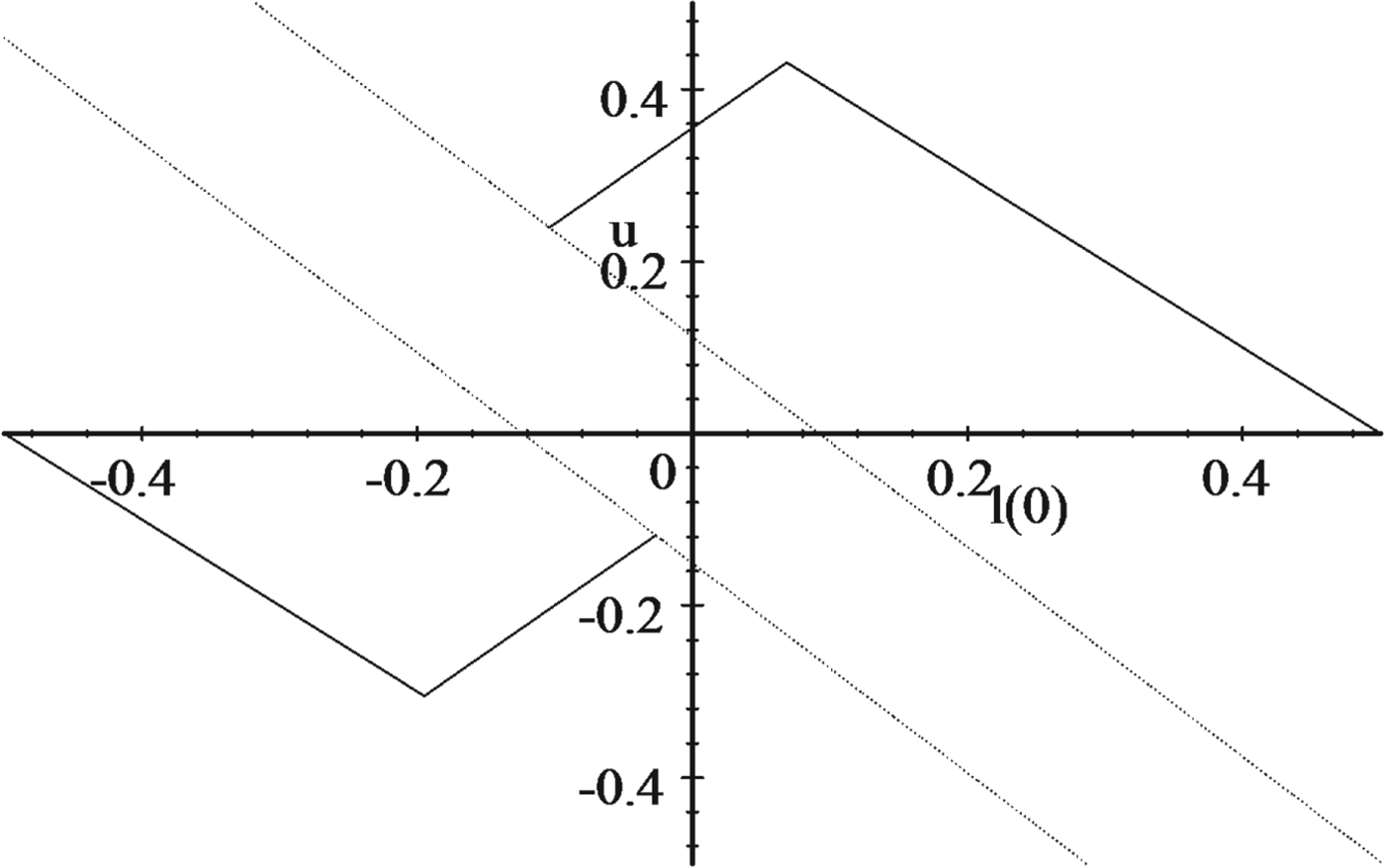
Figure A7 shows the graph of the equilibrium migration correspondence for k 0 = 0.2, G = 0.7, β = 0.8, and γ = 5.
The equilibrium first period migration (u) as a function of l 0 for β = 0.8, γ = 5, G = 0.7 and k 0 = 0.2.

The top kinked line is the graph of min{x,.5 − l 0} over the interval where x ≥ q. The kink occurs where x = .5 − l 0. The top straight line is the graph of q. The bottom kinked line and the bottom straight line are the graphs of max{y, − .5 − l 0} and of p, respectively. The overlap of the two kinked lines defines the ROM, given k 0 = 0.2. If, for example, l 0 = −0.05, the two equilibrium values of migration are u=−0.144 (a movement to Agriculture) and u=0.3 (a movement to Manufacturing).
Our assumptions β 2Gγ > 1 and β ≤ 1 imply that Gγ > 1, so the slope x and y (as functions of l 0) are always positive, as shown. We noted above that inequality (6) implies that the slope of p and q (graphed as functions of l 0) is negative. Therefore, if x ≥ p is satisfied, it holds for large values of l 0; if y ≤ q is satisfied, it holds for small l 0.
The boundaries of the overlap are determined by the solution to x=q and y = p. Denote X(k 0) as the value of l 0 that satisfies x=q, and denote Y(k 0) as the value of l 0 that satisfies y=p. Some calculation yields the formulae in equation (7) of the text. This step establishes part (ii) of the Proposition.
The vertical distance between the boundaries of the ROM is M, defined in equation (8). We noted in the text that inequality (6) and the assumption γβ 2G > 1 imply that χ > 0. Therefore, when these two inequalities hold, the ROM has positive measure. This fact establishes sufficiency in part (i) of the Proposition. The denominator of M is quadratic in γ and the numerator is linear, so M → 0 as γ → ∞. Thus, the measure of the ROM approaches 0 as γ → ∞. Since the measure is 0 for γβ 2G < 1, positive for γβ 2G > 1 and approaches 0 as γ → ∞, it is non-monotonic in γ, as part (iii) of the Proposition states.