


INTRODUCTION
Estimation of ideological positions among voters, legislators, justices, and other actors is central to many subfields of political science. Since the pioneering work of Poole and Rosenthal (Reference Poole and Rosenthal1991, Reference Poole and Rosenthal1997), a number of scholars have used spatial voting models to estimate ideological preferences from roll-call votes and other data in the fields of comparative politics and international relations as well as American politics (e.g., Bailey, Kamoie, and Maltzman Reference Bailey, Kamoie and Maltzman2005; Bailey, Strezhnev, and Voeten Reference Bailey, Strezhnev and Voeten2015; Bonica Reference Bonica2014; Clinton and Lewis Reference Clinton and Lewis2008; Hix, Noury, and Roland Reference Hix, Noury and Roland2006; Ho and Quinn Reference Ho and Quinn2010; Londregan Reference Londregan2007; McCarty, Poole, and Rosenthal Reference McCarty, Poole and Rosenthal2006; Morgenstern Reference Morgenstern2004; Spirling and McLean Reference Spirling and McLean2007; Voeten Reference Voeten2000). These and other substantive applications are made possible by numerous methodological advancements including Bayesian estimation (Clinton, Jackman, and Rivers Reference Clinton, Jackman and Rivers2004; Jackman Reference Jackman2001), optimal classification (Poole Reference Poole2000), dynamic modeling (Martin and Quinn Reference Martin and Quinn2002), and models with agenda setting or strategic voting (Clinton and Meirowitz Reference Clinton and Meirowitz2003; Londregan Reference Londregan1999).
With the increasing availability of data and methodological sophistication, researchers have recently turned their attention to the estimation of ideological preferences that are comparable across time and institutions. For example, Bailey (Reference Bailey2007) measures ideal points of U.S. presidents, senators, representatives, and Supreme Court justices on the same scale over time (see also Bailey Reference Bailey2013; Bailey and Chang Reference Bailey and Chang2001). Similarly, Shor and McCarty (Reference Shor and McCarty2011) compute the ideal points of the state legislators from all U.S. states and compares them with members of Congress (see also Battista, Peress, and Richman Reference Battista, Peress and Richman2013; Shor, Berry, and McCarty Reference Shor, Berry and McCarty2011). Finally, Bafumi and Herron (Reference Bafumi and Herron2010) estimate the ideological positions of voters and their members of Congress in order to study representation while Clinton et al. (Reference Clinton, Bertelli, Grose, Lewis and Nixon2012) compare the ideal points of agencies with those of presidents and congressional members.
Furthermore, researchers have begun to analyze large data sets of various types. For example, Slapin and Proksch (Reference Slapin and Proksch2008) develop a statistical model that can be applied to estimate ideological positions from textual data. Proksch and Slapin (Reference Proksch and Slapin2010) and Lowe et al. (Reference Lowe, Benoit, Mikhaylov and Laver2011) apply this and other similar models to the speeches of European Parliament and the manifestos of European parties, respectively (see also Kim, Londregan, and Ratkovic Reference Kim, Londregan and Ratkovic2014, who analyze the speeches of legislators in U.S. Congress). Another important new data source is social media, which often come in massive size. Bond and Messing (Reference Bond and Messing2015) estimate the ideological preferences of 6.2 million Facebook users while Barberá (Reference Barberá2015) analyze more than 40 million Twitter users. These social media data are analyzed as network data, and a similar approach is taken to estimate ideal points from data on citations using court opinions (Clark and Lauderdale Reference Clark and Lauderdale2010) and campaign contributions from voters to politicians (Bonica Reference Bonica2014).
These new applications pose a computational challenge of dealing with data sets that are orders of magnitude larger than the canonical single-chamber roll-call matrix for a single time period. Indeed, as Table 1 shows, the past decade has witnessed a significant rise in the use of large and diverse data sets for ideal point estimation. While most of the aforementioned works are based on Bayesian models of ideal points, standard Markov chain Monte Carlo (MCMC) algorithms can be prohibitively slow when applied to large data sets. As a result, researchers are often unable to estimate their models using the entire data and are forced to adopt various shortcuts and compromises. For example, Shor and McCarty (Reference Shor and McCarty2011) fit their model in multiple steps using subsets of the data whereas Bailey (Reference Bailey2007) resorts to a simpler parametric dynamic model in order to reduce computational costs (p. 441) (see also Bailey Reference Bailey2013). Since a massive data set implies a large number of parameters under these models, the convergence of MCMC algorithms also becomes difficult to assess. Bafumi and Herron (Reference Bafumi and Herron2010), for example, express a concern about the convergence of ideal points for voters (footnote 24).
Recent Applications of Ideal Point Models to Various Large Data Sets

Notes: The past decade has witnessed a significant rise in the use of large data sets for ideal point estimation. Note that “# of subjects” should be interpreted as the number of ideal points to be estimated. For example, if a legislator serves for two terms and are allowed to have different ideal points in those terms, then this legislator is counted as two subjects.
In addition, estimating ideal points over a long period of time often imposes a significant computational burden. Indeed, the use of computational resources at supercomputer centers has been critical to the development of various NOMINATE scores.Footnote 1 Similarly, estimation of the Martin and Quinn (Reference Martin and Quinn2002) ideal point estimates for U.S. Supreme Court justices over 47 years took over five days to estimate. This suggests that while these ideal point models are attractive, they are often practically unusable for many researchers who wish to analyze a large-scale data set.
In this article, we propose a fast estimation method for ideal points with massive data. Specifically, we develop the Expectation-Maximization (EM) algorithms (Dempster, Laird, and Rubin Reference Dempster, Laird and Rubin1977) that either exactly or approximately maximize the posterior distribution under various ideal point models. The main advantage of EM algorithms is that they can dramatically reduce computational time. Through a number of empirical and simulation examples, we demonstrate that in cases where a standard MCMC algorithm would require several days to compute ideal points, the proposed algorithm can produce essentially identical estimates within minutes. The EM algorithms also scale much better than other existing ideal point estimation algorithms. They can estimate an extremely large number of ideal points on a laptop within a few hours whereas current methodologies would require the level of computational resources only available at a supercomputer center to do the same computation.
We begin by deriving the EM algorithm for the standard Bayesian ideal point model of Clinton, Jackman, and Rivers (Reference Clinton, Jackman and Rivers2004). We show that the proposed algorithm produces ideal point estimates which are essentially identical to those from other existing methods. We then extend our approach to other popular ideal point models that have been developed in the literature. Specifically, we develop an EM algorithm for the model with mixed ordinal and continuous outcomes (Quinn Reference Quinn2004) by applying a certain transformation to the original parametrization. We also develop an EM algorithm for the dynamic model (Martin and Quinn Reference Martin and Quinn2002) and the hierarchical model (Bafumi et al. Reference Bafumi, Gelman, Park and Kaplan2005). Finally, we propose EM algorithms for ideal point models based on textual and network data.
For dynamic and hierarchical models as well as the models for textual and network data, an EM algorithm that directly maximizes the posterior distribution is not available in a closed form. Therefore, we rely on variational Bayesian inference, which is a popular machine learning methodology for fast and approximate Bayesian estimation (see Wainwright and Jordan (Reference Wainwright and Jordan2008) for a review and Grimmer (Reference Grimmer2011) for an introductory article in political science). For each case, we demonstrate the computational efficiency and scalability of the proposed methodology by applying it to a wide range of real and simulated data sets. Our proposed algorithms complement a recent application of variational inference to combine ideal point estimation with topic models (Gerrish and Blei Reference Gerrish and Blei2012). We implement the proposed algorithms via an open-source R package, emIRT (Imai, Lo, and Olmsted Reference Imai, Lo and Olmsted2015), so that others can apply them to their own research.
In the item response theory literature, the EM algorithm is used to maximize the marginal likelihood function where ability parameters, i.e., ideal point parameters in the current context, are integrated out (Bock and Aitkin Reference Bock and Aitkin1981). In the ideal point literature, Bailey (Reference Bailey2007) and Bailey and Chang (Reference Bailey and Chang2001) use variants of the EM algorithm in their model estimation. The M steps of these existing algorithms, however, do not have a closed-form solution. In this article, we derive closed-form EM algorithms for popular Bayesian ideal point models. This leads to faster and more reliable estimation algorithms.
Finally, an important and well-known drawback of these EM algorithms is that they do not produce uncertainty estimates such as standard errors. In contrast, the MCMC algorithms are designed to fully characterize the posterior, enabling the computation of uncertainty measures for virtually any quantities of interest. Moreover, the standard errors based on variational posterior are often too small, underestimating the degree of uncertainty. While many applied researchers tend to ignore estimation uncertainty associated with ideal points, such a practice can yield misleading inference. To address this problem, we apply the parametric bootstrap approach of Lewis and Poole (Reference Lewis and Poole2004) (see also Carroll et al. Reference Carroll, Lewis, Lo and Poole2009). Although this obviously increases the computational cost of the proposed approach, the proposed EM algorithms still scale much better than the existing alternatives. Furthermore, researchers can reduce this computational cost by a parallel implementation of bootstrap on a distributed system. We note that since our models are Bayesian, it is rather unconventional to utilize bootstrap, which is a frequentist procedure. However, one can interpret the resulting confidence intervals as a measure of uncertainty of our Bayesian estimates over repeated sampling under the assumed model.
STANDARD IDEAL POINT MODEL
We begin by deriving the EM algorithm for the standard ideal point model of Clinton, Jackman, and Rivers (Reference Clinton, Jackman and Rivers2004). In this case, the proposed EM algorithm maximizes the posterior distribution without approximation. We illustrate the computational efficiency and scalability of our proposed algorithm by applying it to roll-call votes in recent U.S. Congress sessions, as well as to simulated data.
The Model
Suppose that we have N legislators and J roll calls. Let yij denote the vote of legislator i on roll call j where yij = 1 (yij = 0) implies that the vote is in the affirmative (negative) with i = 1, . . ., N and j = 1, . . ., J. Abstentions, if present, are assumed to be ignorable such that these votes are missing at random and can be predicted from the model using observed data (see Rosas and Shomer Reference Rosas and Shomer2008). Furthermore, let x i represent the K-dimensional column vector of ideal point for legislator i. Then, if we use y* ij to represent a latent propensity to cast a “yea” vote where yij = 1{y* > 0}, the standard K-dimensional ideal point model is given by
 $$\begin{equation}
y_{ij}^\ast \ = \ \alpha _j + \mathbf {x}_i^\top \bm{\beta }_j + \epsilon _{ij},
\end{equation}$$
where β j is the K-dimensional column vector of item discrimination parameters and α j is the scalar item difficulty parameter. Finally, ε ij is an independently, identically distributed random utility and is assumed to follow the standard normal distribution.
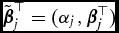
For notational simplicity, we use
 $\tilde{\bm{\beta }}_j^\top =(\alpha _j,\bm{\beta }_j^\top )$
and
 $\tilde{\mathbf {x}}_i^\top = (1, \mathbf {x}_i^\top )$
so that equation (1) can be more compactly written as
 $$\begin{eqnarray}
y_{ij}^\ast & = & \tilde{\mathbf {x}}_i^\top \tilde{\bm{\beta }}_j + \epsilon _{ij}.
\end{eqnarray}$$
Following the original article, we place independent and conjugate prior distributions on x
i
and
 $\tilde{\bm{\beta }}_j$
, separately. Specifically, we use
 $$\begin{eqnarray}
p(\mathbf {x}_1,\dots ,\mathbf {x}_N) \ &=& \ \prod _{i=1}^{N} \phi _K \left(\mathbf {x}_i; \bm{\mu }_{\mathbf {x}} , \bm{\Sigma }_{\mathbf {x}} \right) \quad {\rm and} \quad \nonumber\\
p(\tilde{\bm{\beta }}_1,\dots ,\tilde{\bm{\beta }}_J) \ &=& \ \prod _{j=1}^{J} \phi _{K+1} \left(\tilde{\bm{\beta }}_j; \bm{\mu }_{\tilde{\bm{\beta }}} , \bm{\Sigma }_{\tilde{\bm{\beta }}} \right),
\end{eqnarray}$$
where ϕ
k
(·;·) is the density of a k-variate Normal random variable,
μ
x
and
 $\bm{\mu }_{\tilde{\bm{\beta }}}$
represent the prior mean vectors, and
Σ
x
and
 $\bm{\Sigma }_{\tilde{\bm{\beta }}}$
are the prior covariance matrices.
Given this model, the joint posterior distribution of
 $(\mathbf {Y}^\ast ,\lbrace \mathbf {x}_i\rbrace _{i=1}^N,\lbrace \tilde{\bm{\beta }}_j\rbrace _{j=1}^J)$
conditional on the roll-call matrix Y is given by
 $$\begin{eqnarray}
&& p\left(\mathbf {Y}^\ast ,\lbrace \mathbf {x}_i\rbrace _{i=1}^N,\lbrace \tilde{\bm{\beta }}_j\rbrace _{j=1}^J \mid \mathbf {Y}\right) \nonumber \\
&&\quad \propto \ \prod _{i=1}^N \prod _{j=1}^J \left( \mathbf {1}\lbrace y_{ij}^\ast > 0\rbrace \mathbf {1}\lbrace y_{ij} = 1\rbrace\right.\nonumber\\
&&\quad \left.\quad + \, \mathbf {1}\lbrace y_{ij}^\ast \le 0\rbrace \mathbf {1}\lbrace y_{ij} = 0\rbrace \right)\ \phi _1\left(y_{ij}^\ast ; \tilde{\mathbf {x}}_i^\top \tilde{\bm{\beta }}_j, 1\right) \nonumber \\
\quad \times \, \prod _{i=1}^{N} \phi _K \left(\mathbf {x}_i; \bm{\mu }_{\mathbf {x}} , \bm{\Sigma }_{\mathbf {x}} \right) \prod _{j=1}^{J} \phi _{K+1} \left(\tilde{\bm{\beta }}_j; \bm{\mu }_{\tilde{\bm{\beta }}} , \bm{\Sigma }_{\tilde{\bm{\beta }}} \right),\quad
\end{eqnarray}$$
where Y and Y* are matrices whose element in the ith row and jth column is yij and y* ij , respectively. Clinton, Jackman, and Rivers (Reference Clinton, Jackman and Rivers2004) describe the MCMC algorithm to sample from this joint posterior distribution and implement it as the ideal() function in the open-source R package pscl (Jackman Reference Jackman2012).
The Proposed Algorithm
We derive the EM algorithm that maximizes the posterior distribution given in equation (4) without approximation. The proposed algorithm views {x
i
}
N
i = 1 and
 $\lbrace \tilde{\bm{\beta }}_j\rbrace _{j=1}^J$
as parameters and treats Y* as missing data. Specifically, at the tth iteration, denote the current parameter values as {x
(t − 1)
i
}
i = 1
N
and
 $\lbrace \tilde{\bm{\beta }}_j^{(t-1)}\rbrace _{j=1}^J$
. Then, the E step is given by the following so-called “Q function,” which represents the expectation of the log joint posterior distribution,
 $$\begin{eqnarray}
Q(\lbrace \mathbf {x}_i\rbrace _{i=1}^N, \lbrace \tilde{\bm{\beta }}_j\rbrace _{j=1}^J)\nonumber \\
\quad = \mathbb {E}\left[\log p(\mathbf {Y}^\ast ,\lbrace \mathbf {x}_i\rbrace _{i=1}^N,\lbrace \tilde{\bm{\beta }}_j\rbrace _{j=1}^J \mid \mathbf {Y}) \mid \mathbf {Y},\right.\nonumber\\
\left.\qquad\quad \lbrace \mathbf {x}_i^{(t-1)}\rbrace _{i=1}^N, \lbrace \tilde{\bm{\beta }}_j^{(t-1)}\rbrace _{j=1}^J \right] \nonumber \\
\quad = \,- \frac{1}{2} \sum _{i=1}^N \sum _{j=1}^J \left(\tilde{\bm{\beta }}_j^\top \tilde{\mathbf {x}}_i \tilde{\mathbf {x}}_i^\top \tilde{\bm{\beta }}_j - 2 \tilde{\bm{\beta }}_j^\top \tilde{\mathbf {x}}_i {y_{ij}^\ast }^{(t)}\right)\nonumber\\
\qquad\,- \frac{1}{2} \sum _{i=1}^N \left(\mathbf {x}_i^\top \bm{\Sigma }_\mathbf {x}^{-1} \mathbf {x}_i - 2 \mathbf {x}_i^\top \bm{\Sigma }_\mathbf {x}^{-1} \bm{\mu }_\mathbf {x}\right) \nonumber \\
\qquad\,- \frac{1}{2} \sum _{j=1}^J \left(\tilde{\bm{\beta }}_j^\top \bm{\Sigma }_{\tilde{\bm{\beta }}}^{-1} \tilde{\bm{\beta }}_j - 2 \tilde{\bm{\beta }}_j^\top \bm{\Sigma }_{\tilde{\bm{\beta }}}^{-1} \bm{\mu }_{\tilde{\bm{\beta }}}\right) + \mathrm{const.}\\[-25pt]
\nonumber
\end{eqnarray}$$
where
 $$\begin{eqnarray}
{y_{ij}^\ast }^{(t)} \ &=& \ \mathbb {E}\left(y_{ij}^\ast \mid \mathbf {x}_i^{(t-1)}, \tilde{\bm{\beta }}_j^{(t-1)}, y_{ij}\right)\nonumber\\
& = & \left\lbrace \arraycolsep5pt\begin{array}{@{}ll@{}}m_{ij}^{(t-1)} + \frac{\phi (m_{ij}^{(t-1)})}{\Phi (m_{ij}^{(t-1)})} & \textrm {if}\, y_{ij} = 1 \\
m_{ij}^{(t-1)} - \frac{\phi (m_{ij}^{(t-1)})}{1-\Phi (m_{ij}^{(t-1)})} & \textrm {if}\, y_{ij} = 0 \\
m_{ij}^{(t-1)} & \textrm {if}\, y_{ij} \textrm { is missing} \end{array}\right.
\end{eqnarray}$$
with
 $m_{ij}^{(t-1)}=(\tilde{\mathbf {x}}_i^{(t-1)})^\top \tilde{\bm{\beta }}_j^{(t-1)}$
.
Straightforward calculation shows that the maximization of this Q function, i.e., the M step, can be achieved via the following two conditional maximization steps:
 $$\begin{eqnarray}
\mathbf {x}_i^{(t)} &=& \left(\bm{\Sigma }_\mathbf {x}^{-1} + \sum _{j=1}^J \bm{\beta }_j^{(t-1)}{\bm{\beta }_j^{(t-1)}}^\top \right)^{-1}\nonumber\\
&&\times \left( \bm{\Sigma }_\mathbf {x}^{-1}\bm{\mu }_\mathbf {x}+ \sum _{j=1}^J \bm{\beta }_j^{(t-1)}({y_{ij}^\ast }^{(t)} - \alpha _j^{(t-1)})\right),
\end{eqnarray}$$
 $$\begin{eqnarray}
\tilde{\bm{\beta }}_j^{(t)} &=& \left(\bm{\Sigma }_{\tilde{\bm{\beta }}}^{-1} + \sum _{i=1}^N \tilde{\mathbf {x}}_i^{(t)}\left(\tilde{\mathbf {x}}_i^{(t)}\right)^\top \right)^{-1}\nonumber\\
&&\times \left( \bm{\Sigma }_{\tilde{\bm{\beta }}}^{-1}\bm{\mu }_{\tilde{\bm{\beta }}} + \sum _{i=1}^N \tilde{\mathbf {x}}_i^{(t)}{y_{ij}^\ast }^{(t)} \right).
\end{eqnarray}$$
The algorithm repeats these E and M steps until convergence. Given that the model is identified up to an affine transformation, we use a correlation-based convergence criteria where the algorithm terminates when the correlation between the previous and current values of all parameters reaches a prespecified threshold.Footnote 2
Finally, to compute uncertainty estimates, we apply the parametric bootstrap (Lewis and Poole Reference Lewis and Poole2004). Specifically, we first estimate ideal points and bill parameters via the proposed EM algorithm. Using these estimates, we calculate the choice probabilities associated with each outcome. Then, we randomly generate roll-call matrices given these estimated outcome probabilities. Where there are missing votes, we simply induce the same missingness patterns. This is repeated a sufficiently large number of times and the resulting bootstrap replicates for each parameter are used to characterize estimation uncertainty.
An Empirical Application
To assess its empirical performance, we apply the proposed EM algorithm to roll-call voting data for both the Senate and the House of Representatives for sessions of Congress 102 through 112. Specifically, we compare the ideal point estimates and their computation time from the proposed algorithm to those from three other methods; the MCMC algorithm implemented as ideal() in the R package pscl (Jackman Reference Jackman2012), the alternating maximum likelihood estimator implemented as wnominate() in the R package wnominate (Poole et al. Reference Poole, Lewis, Lo and Carroll2011), and the nonparametric optimal classification estimator implemented as oc() in the R package oc (Poole et al. Reference Poole, Lewis, Lo and Carroll2012). For all roll-call matrices, we restrict attention to just those legislators with at least 25 observed votes on nonunanimous bills. In all cases, we assume a single spatial dimension.
We caution that the comparison of computational efficiency presented here is necessarily illustrative. The performance of any numerical algorithm may depend on starting values, and no absolute convergence criteria exists for any of the algorithms we examine. For the MCMC algorithm, we run the chain for 100,000 iterations beyond a burn-in period of 20,000 iterations. Inference is based on a thinned chain where we keep every 100 draws. While the length of chain and its thinning interval are within the recommended range by Clinton, Jackman, and Rivers (Reference Clinton, Jackman and Rivers2004), we emphasize that any convergence criteria used for deciding when to terminate the MCMC algorithm is somewhat arbitrary. The default diffuse priors, specified in ideal() from the R package pscl, are used and propensities for missing votes are not imputed during the data-augmentation step. In particular, we assume a single dimensional normal prior for all ideal point parameters with a mean of 0 and a variance of 1. For the bill parameters, we assume a two-dimensional normal prior with a mean vector of 0’s and a covariance matrix with each variance term equal to 25 and no covariance. The standard normalization of ideal points, i.e., a mean of 0 and a standard deviation of 1, is used for local identification. The MCMC algorithm produces measures of uncertainty for the parameter estimates and so we distinguish it from those algorithms which produce only point estimates by labeling it in Figure 1 with bold, italic typeface.
Comparison of Computational Performance across the Methods

For the proposed EM algorithm, we use random starting values for the ideal point and bill parameters. The same prior distributions as the MCMC algorithm are used for all parameters. We terminate the EM algorithm when each block of parameters has a correlation with the values from the previous iteration larger than 1 − p. With one spatial dimension, we have three parameter blocks: the bill difficulty parameters, the bill discrimination parameters and the ideal point parameters. Following Poole and Rosenthal (Reference Poole and Rosenthal1997) (see p. 237), we use p = 10−2. We also consider a far more stringent criterion where p = 10−6, requiring parameters to correlate greater than 0.999999. In the following results, we focus on the latter “high precision” variant, except in the case of computational performance where results for both criteria are presented (labeled “EM” and “EM (high precision),” respectively). The results from the EM algorithm do not include measures of uncertainty. For this, we include the “EM with Bootstrap” variant which uses 100 parametric bootstrap replicates. To distinguish this algorithm from those which produce just point estimates, it is labeled in Figure 1 with bold, italic typeface.
Finally, for W-NOMINATE, we do not include any additional bootstrap trials for characterizing uncertainty about the parameters, so the results will only include point estimates. For optimal classification, we use the default setting of oc() in the R package oc. Because the Bayesian MCMC algorithm is stochastic and the EM algorithm has random starting values, we run each estimator 50 times for any given roll-call matrix and report the median of each performance measurement.
We begin by examining the computational performance of the EM algorithm.Footnote 3 Figure 1 shows the time required for the ideal point estimation for each Congressional session in the House (left panel) and the Senate (right panel). Note that the vertical axis is on the log scale. Although the results are only illustrative for the aforementioned reasons, it is clear that the EM algorithm is by far the fastest. For example, for the 102nd House of Representatives, the proposed algorithm, denoted by “EM,” takes less than one second to compute estimates, using the same convergence criteria as W-NOMINATE. Even with a much more stringent convergence criteria “EM (high-precision),” the computational time is only six seconds. This contrasts with the other algorithms, which require much more time for estimation. Although the direct comparison is difficult, the MCMC algorithm is by far the slowest, taking more than 2.5 hours. Because the MCMC algorithm produces standard errors, we contrast the performance of “IDEAL” with “EM with Bootstrap” and find that obtaining 100 bootstrap replicates requires just under one minute. Even if more iterations are desired, over 10,000 bootstrap iterations could be computed before approaching the time required by the MCMC algorithm.
The W-NOMINATE and optimal classification estimators are faster than the MCMC algorithm but take approximately one and 2.5 minutes, respectively. These methods do not provide measures of uncertainty, and all of the point-estimate EM variants are over ten times faster. Last, the EM algorithm is amenable to parallelization within each of the three update steps. The open-source implementation that we provide supports this on some platforms (Imai, Lo, and Olmsted Reference Imai, Lo and Olmsted2015). And, the parallelized implementation performs well. For any of these roll-call matrices, using eight processor cores to estimate the parameters instead of just one core reduces the required timeto completion to about one-sixth of the single core time.
We next show that the computational gain of the proposed algorithm is achieved without sacrificing the quality of estimates. To do so, we directly compare individual-level ideal point estimates across the methods. Figure 2 shows, using the 112th Congress, that except for a small number of legislators, the estimates from the proposed EM algorithm are essentially identical to those from the MCMC algorithm (left column) and W-NOMINATE (right column). The within-party correlation remains high across the plots, indicating that a strong agreement among these estimates up to affine transformation.Footnote 4 The agreement with the results based on the MCMC algorithm is hardly surprising given that both algorithms are based on the same posterior distribution. The comparability of estimates across methods holds for the other sessions of Congress considered.
Comparison of Estimated Ideal Points across the Methods for the 112th Congress

For a small number of legislators, the deviation between results for the proposed EM algorithm and both the MCMC algorithm and W-NOMINATE is not negligible. However, this is not a coincidence—it results from the degree of missing votes associated with each legislator.Footnote 5 The individuals for whom the estimates differ significantly all have no position registered for more than 40% of the possible votes. Examples include President Obama, the late Congressman Donald Payne (Democrat, NJ), and Congressman Thomas Massie (Republican, KY).Footnote 6 With a small amount of data, the estimation of these legislators’ ideal points is sensitive to the differences in statistical methods.
We also compare the standard errors from the proposed EM algorithm using the parametric bootstrap with those from the MCMC algorithm. Because the output from the MCMC algorithm is rescaled to have a mean of zero and standard deviation of 1, we rescale the EM estimates to have the same sample moments. This affine transformation is applied to each bootstrap replicate so that the resulting bootstrap standard errors are on the same scale as those based on the MCMC algorithm. Figure 3 does this comparison using the estimates for the 112th House of Representatives. The left panel shows that the standard errors based on the EM algorithm with the bootstrap (the vertical axis) are only slightly smaller than those from the MCMC algorithm (the horizontal axis) for most legislators. However, for a few legislators, the standard errors from the EM algorithm are substantially smaller than those from the MCMC algorithm. The right panel of the figure shows that these legislators have extreme ideological preferences.
Comparison of Standard Errors between the Proposed EM Algorithm and the Bayesian MCMC Algorithm using the 112th House of Representatives

To further examine the frequentist properties of our standard errors based on parametric bootstrap, we conduct a Monte Carlo simulation where roll-call votes are simulated consistent with data from the 112th House of Representatives. That is, we use the estimates obtained from these data as truths and simulate roll-call data 1,000 times according to the model. When simulating the data, the same missingness pattern as the observed data from the 112th Congress is used. For each of the 1,000 simulated roll call data sets, we estimate the ideal points and compute the standard error based on 100 parametric bootstrap replicates. We then estimate the bias of the resulting standard error for each legislator as the average difference between the bootstrap standard error and the standard deviation of estimated ideal points across 1,000 simulations.
Figure 4 shows the estimated biases. The left panel of the figure shows that the biases of the standard errors are not systematically related to the extremity of ideological positions. Thus, the divergence between the MCMC and parametric bootstrap standard errors for extreme legislators observed in Figure 3 does not necessarily suggest that the latter is underestimated. Instead, as shown in the right panel of Figure 4, the biases of parametric bootstrap standard errors are driven by the amount of missing data. The plot shows that the standard errors are significantly underestimated for those legislators with a large amount of missing data.
Bias of Standard Error based on the Parametric Bootstrap

Simulation Evidence
Next, we use Monte Carlo simulation to assess the computational scalability of the proposed EM algorithm as the dimensions of the roll-call matrix get larger. The empirical application in the previous subsection demonstrated the poor scalability of the MCMC algorithm. Hence, we compare the performance of our algorithm with W-NOMINATE. Figure 5 shows the median performance of both the EM algorithm with high precision and “W-NOMINATE” over 25 Monte Carlo trials for various numbers of legislators and bills. In the left panel, the number of bills is fixed at 1,000 and the number of legislators ranges from 50 to 10,000. In the right panel, the number of legislators is fixed at 500, and the number of bills ranges from 50 to 5,000. In both cases, the data-generating process follows the single dimensional ideal point model where ideal points are generated according to the standard normal distribution and the bill parameters follow from a normal distribution with mean zero and standard deviation of 10. These parameter values are chosen so that the true parameter values explain around 85% percent of the observed votes—a level of classification success comparable to the in-sample fit obtained in contemporary sessions of Congress.
Comparison of Changing Performance across the Methods as the Dimensions of Roll-Call Matrix Increase

The computational efficiency of the proposed algorithm can be seen immediately. Even with 10,000 legislators and 1,000 bills, convergence at high precision is achieved in less than 15 minutes. The runtime of our algorithm increases only linearly as the number of ideal points increases. This contrasts with W-NOMINATE, whose required computation time grows exponentially as the number of legislators increases. For example, both the EM algorithm and W-NOMINATE require less than 5 minutes to estimate the parameters associated with a roll-call matrix with 1,000 legislators and 1,000 bills. However, when the number of legislators increases to 10,000, W-NOMINATE takes around 2.5 hours while the EM algorithm requires less than 15 minutes. The difference is less stark when the number of bills increase (right panel). Even here, however, the EM algorithm is more computationally efficient, especially when the number of bills is large.
IDEAL POINT MODEL WITH MIXED BINARY, ORDINAL, AND CONTINUOUS OUTCOMES
We extend the EM algorithm developed above to the ideal point model with mixed binary, ordinal, and continuous outcomes. Quinn (Reference Quinn2004) develops an MCMC algorithm for fitting this model and implements it as the MCMCmixfactanal() function in the open-source R package MCMCpack (Martin, Quinn, and Park Reference Martin, Quinn and Park2013). The EM algorithm for the ordinal probit model, which is closely related to this model, poses a special challenge because its E step is not available in closed form. Perhaps for this reason, to the best of our knowledge, the EM algorithm has not been developed for the ordinal probit model in the statistics literature.
In this section, we first show that the E step can be derived in a closed form so long as the outcome variable only has three ordinal categories. With a suitable transformation of parameters, we derive an EM algorithm that is analytically tractable. We then consider the cases where the number of categories in the outcome variable exceeds three and the outcome variable is a mix of binary, ordinal, and continuous variables. Finally, we apply the proposed algorithm to a survey of Japanese politicians and voters.
The Model with a Three-category Ordinal Outcome
We consider the same exact setup as the standard model introduced above, with the exception that the outcome variable now takes one of the three ordered values, i.e., yij ∈ {0, 1, 2}. In this model, the probability of each observed choice is given as follows:
 $$\begin{equation}
\Pr (y_{ij} = 0) \ = \ \Phi (\alpha _{1j} - \mathbf {x}_i^\top \bm{\beta }_j),
\end{equation}$$
 $$\begin{eqnarray}
\Pr (y_{ij} = 1) \ = \ \Phi (\alpha _{2j} - \mathbf {x}_i^\top \bm{\beta }_j) - \Phi (\alpha _{1j} - \mathbf {x}_i^\top \bm{\beta }_j),\quad
\end{eqnarray}$$
 $$\begin{eqnarray}
\Pr (y_{ij} = 2) \ = \ 1 - \Phi (\alpha _{2j} - \mathbf {x}_i^\top \bm{\beta }_j),
\end{eqnarray}$$
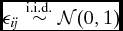
where α2j > α1j for all j = 1, 2, . . ., J. The model can be written using the latent propensity to agree y* ij for respondent i as
 $$\begin{eqnarray}
y^\ast _{ij} & \ = \ \mathbf {x}_i^\top \bm{\beta }_j + \epsilon _{ij},
\end{eqnarray}$$
where
 $\epsilon _{ij} \stackrel{\rm i.i.d.}{\sim }\mathcal {N}(0,1)$
and these latent propensities are connected to the observed outcomes through the following relationship:
 $$\begin{eqnarray}
y_{ij} \ = \ \left\lbrace \begin{array}{@{}ll@{}}0 & \text{if} \ \ y_{ij}^\ast < \alpha _{1j} \\
1 & \text{if} \ \ \alpha _{1j} \le y_{ij}^\ast < \alpha _{2j} \\
2 & \text{if} \ \ \alpha _{2j} \le y_{ij}^\ast \end{array}\right..
\end{eqnarray}$$
As in the standard ideal point model, we treat abstention as missing at random.
Following the literature, we assume the same normal independent prior distribution on ({ β j } J j = 1, {x i } N i = 1) as the one used for the standard binary model. For ({α1j , α2j } J j = 1), we assume an improper uniform prior with the appropriate ordering restriction α1j < α2j . Then, the joint posterior distribution is given by
 $$\begin{eqnarray}
&& p(\mathbf {Y}^\ast , \lbrace \mathbf {x}_i\rbrace _{i=1}^N, \lbrace \alpha _{1j},\alpha _{2j},\bm{\beta }_j\rbrace _{j=1}^J \mid \mathbf {Y}) \nonumber \\
&&\propto \ \prod _{i=1}^N \prod _{j=1}^J \left[\mathbf {1}\lbrace y_{ij}^\ast < \alpha _{1j}\rbrace \mathbf {1}\lbrace y_{ij}=0\rbrace\right.\nonumber\\
&&\left.\quad \,+\, \mathbf {1}\lbrace \alpha _{1j} \le y_{ij}^\ast < \alpha _{2j}\rbrace \mathbf {1}\lbrace y_{ij}=1\rbrace\right.\nonumber\\
&&\left.\quad \,+\, \mathbf {1}\lbrace y_{ij}^\ast \ge \alpha _{2j}\rbrace \mathbf {1}\lbrace y_{ij}=2\rbrace \right] \phi _1(y_{ij}^\ast ; \mathbf {x}_i^\top \bm{\beta }_j, 1) \nonumber \\
&&\quad \,\times\, \prod _{i=1}^N \phi _K(\mathbf {x}_i; \bm{\mu }_\mathbf {x}, \bm{\Sigma }_\mathbf {x}) \prod _{j=1}^J \phi _K(\bm{\beta }_j; \bm{\mu }_{\bm{\beta }}, \bm{\Sigma }_{\bm{\beta }}).
\end{eqnarray}$$
The Proposed Algorithm
To develop an EM algorithm that is analytically tractable, we employ the following one-to-one transformation of parameters:
 $$\begin{eqnarray}
\tau _j = \alpha _{2j} - \alpha _{1j} \ > \ 0,
\end{eqnarray}$$
 $$\begin{eqnarray}
\alpha _{j}^\ast = -\frac{\alpha _{1j}}{\tau _j},
\end{eqnarray}$$
 $$\begin{eqnarray}
\bm{\beta }_j^\ast = \frac{\bm{\beta }_j}{\tau _j},
\end{eqnarray}$$
 $$\begin{eqnarray}
z_{ij}^\ast = \frac{y_{ij}^\ast - \alpha _{1j}}{\tau _j},
\end{eqnarray}$$
 $$\begin{eqnarray}
\epsilon _{ij}^\ast = \frac{\epsilon _{ij}}{\tau _j}.
\end{eqnarray}$$
Then, the simple algebra shows that the model can be rewritten as
 $$\begin{eqnarray}
\Pr (y_{ij} = 0) \ = \ \Phi (-\tau _j \alpha _{j}^\ast - \tau _j\mathbf {x}_i^\top \bm{\beta }_j^\ast ),
\end{eqnarray}$$
 $$\begin{eqnarray}
\Pr (y_{ij} = 1) \ &=& \ \Phi (-\tau _j \alpha _j^\ast + \tau _j - \tau _j \mathbf {x}_i^\top \bm{\beta }_j^\ast )\nonumber\\
&& - \Phi (-\tau _j \alpha _j^\ast - \tau _j \mathbf {x}_i^\top \bm{\beta }_j^\ast ),
\end{eqnarray}$$
 $$\begin{eqnarray}
\Pr (y_{ij} = 2) \ = \ 1 - \Phi (-\tau _j \alpha _j^\ast + \tau _j - \tau _j \mathbf {x}_i^\top \bm{\beta }_j^\ast ),
\end{eqnarray}$$
where the latent variable representation is given by
 $$\begin{eqnarray}
z_{ij}^\ast = \alpha _j^\ast + \mathbf {x}_i^\top \bm{\beta }_j^\ast + \epsilon ^\ast {\rm with} \epsilon _{ij}^\ast \stackrel{\rm indep.}{\sim }\mathcal {N}(0,\ \tau _j^{-2}).\quad
\end{eqnarray}$$
Under this parametrization, the relationship between the observed outcome yij and the latent variable z* ij is given by
 $$\begin{eqnarray}
y_{ij} \ = \ \left\lbrace \begin{array}{@{}ll@{}}0 & \text{if} \ \ z_{ij}^\ast < 0 \\
1 & \text{if} \ \ 0 \le z_{ij}^\ast < 1 \\
2 & \text{if} \ \ 1 \le z_{ij}^\ast \end{array}\right..
\end{eqnarray}$$
Thus, the consequence of this reparametrization is that the threshold parameters (α1j , α2j ) are replaced with the intercept term α* j and the heterogeneous variance parameter τ−2 j .
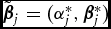
To maintain conjugacy, we alter the prior distribution specified in equation (14). In particular, we use the following prior distribution:
 $$\begin{eqnarray}
&&p\left(\lbrace \tilde{\bm{\beta }}_j\rbrace _{j=1}^J, \left\lbrace \tau _j^2\right\rbrace _{j=1}^J, \lbrace \mathbf {x}_i\rbrace _{i=1}^N\right) = \prod _{j=1}^J \phi _{K+1}(\tilde{\bm{\beta }}_j; \bm{\mu }_{\tilde{\bm{\beta }}}, \bm{\Sigma }_{\tilde{\bm{\beta }}}) \nonumber\\
&&\quad\,\times\, \mathcal{G}\left(\tau _j^2; \frac{\nu _\tau }{2}, \frac{s_\tau }{2}\right) \prod _{i=1}^N \phi _K(\mathbf {x}_i; \bm{\mu }_\mathbf {x}, \bm{\Sigma }_\mathbf {x}),
\end{eqnarray}$$
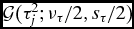
where
 $\tilde{\bm{\beta }}_j = (\alpha _j^\ast , \bm{\beta }_j^\ast )$
and
 $\mathcal {G}(\tau _j^2; \nu _\tau /2, s_\tau /2)$
is the Gamma distribution with ντ/2 > 0 and s
τ/2 > 0 representing the prior shape and rate parameters, respectively. This change in prior distribution alters the model but so long as the prior is diffuse and the size of data is large the resulting inference should not differ much.
Given this setup, we derive the EM algorithm to maximize the posterior distribution. We take the analytical strategy similar to the one used for the standard ideal point model. The resulting algorithm is described in the final section.
Mixed Binary, Ordinal, and Continuous Outcomes
Here we consider how to apply, possibly after some modification, the EM algorithm developed above to a more generel case with mixed binary, ordinal, and continuous outcomes. If the number of ordered categories in outcome exceeds 3, we collapse them into three categories for the sake of analytical tractability and computational efficiency.Footnote 7 For example, responses to a survey question on the five-point Likert scale, i.e., strongly disagree, disagree, neither agree nor disagree, agree, strongly agree, may be converted into a three-point scale by combining strongly disagree and disagree into a single category and strongly agree and agree into another category. Researchers must carefully judge the extent of tradeoff between the loss of information and the computational speed for each application.
Next, suppose that yij is a binary outcome for a particular observation (i, j). Then, we consider the following relationship between this observed outcome and the latent propensity z* ij ; zij < 1⟺yij = 0 and zij ⩾ 0⟺yij = 1. Under this assumption, the E step becomes
 $$\begin{eqnarray}
{z_{ij}^\ast }^{(t)} & \!\!\,=\,\!\! \left\lbrace \begin{array}{@{}ll@{}}m_{ij}^{(t-1)} -\frac{1}{\tau _j^{(t-1)}}\lambda \left(-m_{ij}^{(t-1)}+1, \tau _j^{(t-1)}\right) & \text{if } y_{ij}=0\nonumber\\
m_{ij}^{(t-1)} + \frac{1}{\tau _j^{(t-1)}} \lambda \left(m_{ij}^{(t-1)}, \tau _j^{(t-1)}\right) & \text{if } y_{ij}=1 \end{array}\right.\!\!\!\!\! \\
\end{eqnarray}$$
and
 $$\begin{eqnarray}
\left({z_{ij}^\ast }^2\right)^{(t)}\nonumber\\
\quad = \left\lbrace \begin{array}{@{}ll@{}}\left({z_{ij}^\ast }^{(t)}\right)^2 + \frac{1}{\left(\tau _j^{(t-1)}\right)^2} \left[1 - \frac{1-m_{ij}^{(t-1)}}{\tau _j^{(t-1)}} \lambda\right.\\[4pt]
\quad \left.\times\, \left(m_{ij}^{(t-1)}-1, \tau _j^{(t-1)}\right) \right.\\[4pt]
\quad \left. -\, \left\lbrace \lambda \left(m_{ij}^{(t-1)}-1, \tau _j^{(t-1)}\right)\right\rbrace ^2 \right] \nonumber\\[6pt]
\text{if } y_{ij}=0\\[6pt]
\left({z_{ij}^\ast }^{(t)}\right)^2 + \frac{1}{\left(\tau _j^{(t-1)}\right)^2}\left[1\vphantom{\left(-m_{ij}^{(t-1)}, \tau _j^{(t-1)} \right)} \right.
\left.-\, \lambda \left(-m_{ij}^{(t-1)}, \tau _j^{(t-1)} \right)\right.\\[4pt]
\quad \left.\times\, \left\lbrace \lambda \left(-m_{ij}^{(t-1)}, \tau _j^{(t-1)} \right)\right.\right.
\left.\left. +\, m_{ij}^{(t-1)} \tau _j^{(t-1)} \right\rbrace \right] \nonumber\\[6pt]
\text{if } y_{ij}=1 \end{array}\right., \nonumber\\
\end{eqnarray}$$
where if yij is missing, we set z* ij (t) = mij (t − 1) and (z* ij 2)(t) = (zij *(t))2 + (τ(t − 1) j )−2. Other than these modifications, the rest of the EM algorithm stays identical.
Finally, it is straightforward to extend this model to also include a continuous outcome as done by Quinn (Reference Quinn2004). In that case, set the first and second moments of the latent propensity as z* ij (t) = yij and (z* ij 2)(t) = yij 2 + (τ(t − 1) j )−2 for this observation. The rest of the EM algorithm remains unchanged.
An Empirical Application
We apply the ordinal ideal point model to the survey data of the candidates and voters of Japanese Upper and Lower House elections. This Asahi-Todai Elite survey was conducted by the University of Tokyo in collaboration with a major national newspaper, the Asahi Shimbun, covering all candidates (both incumbents and challengers) for the eight elections that occurred between 2003 and 2013. In six out of eight waves, the survey was also administered to a nationally representative sample of voters with the sample size ranging from approximately 1,100 to about 2,000. The novel feature of the data is that there are a set of common policy questions, which can be used to scale both politicians and voters over time on the same dimension. Another important advantage of the data is a high response rate among politicians, which exceeded 85%. Such a high response rate is obtained in large part because the survey results are published in the Asahi Shimbun whose circulation is approximately eight million (see Hirano et al. Reference Hirano, Imai, Shiraito and Taniguchi2011, for more details).
All together, the data set we analyze contains a total of N = 19,443 respondents, including 7,734 politicians and 11,709 voters. Here, we count multiple appearances of the same politician separately because an ideal point will be estimated separately for each wave. There are J = 98 unique questions in the survey, most of which consisted of questions asking for responses on a five-point Likert scale. We apply the proposed EM algorithm after coarsening each response into three categories (disagree, neutral, and agree). For the purpose of comparison, we developed and used a customized C language implementation of the MCMC algorithm. The data set in this application was too large for MCMCmixfactanal() from the R package MCMCpack to handle. One model uses the full range of categories found in the data without coarsening, and the other model uses the same coarsened responses as done for our algorithm. Obtaining 10,000 draws from the posterior distribution using the MCMC algorithm takes 4 hours and 24 minutes (5 category) or 3 hours and 54 minutes (3 category). In contrast, estimation using our proposed EM algorithm takes 164 iterations and only 68 seconds to complete where the algorithm is iterated until the correlation of parameter values between two consecutive iterations reaches 1 − 10−6.
Figure 6 compares the estimated ideal points of politicians based on our EM algorithm (vertical axis) against those obtained from the standard MCMC algorithm (horizontal axis). As explained earlier, the EM estimates are based on the coarsened three category response, while we present the MCMC estimates using the original five category response (right panel) as well as the same coarsened three category response (left panel). The plots show that these two algorithms produce essentially identical estimates, achieving a correlation greater than 0.95. In addition, for this data set, coarsening the original five category response into a three category response does not appear to have a significant impact on the degree of correlation between the two sets of ideal point estimates of Japanese politicians.
Comparison of Ideal Point Estimates from the EM and Markov Chain Monte Carlo (MCMC) Algorithms for Japanese Politicians Using the Asahi-Todai Elite Survey

Figure 7 compares the estimated ideal points of voters for each wave of survey, obtained from our EM algorithm (white box plots) and the standard MCMC algorithm (light and dark grey box plots for the coarsened three category and original five category responses, respectively). Across all six waves of the survey, the three algorithms give similar distributions of estimated ideal points. The differences across the algorithms lie mostly in their estimated ideal points for a small subset of voters who answer too few questions. For example, the 2003 survey included only two policy questions, and 306 respondents from this survey gave the same two responses. For these respondents, our EM algorithm produces an identical ideal point estimate of − 0.89 whereas the MCMC algorithm gives a set of ideal points ranging from about − 3 to 0, mainly due to the imprecise nature of posterior mean point estimates when votes are not informative. Overall, the results suggest that our EM algorithm recovers virtually identical estimates to those derived via the standard MCMC algorithm but with substantial savings in time.
Comparing the Distributions of Estimated Ideal Points between the EM and Markov Chain Monte Carlo (MCMC) Algorithms for Japanese Voters across Six Waves of the Asahi-Todai Elite Survey

DYNAMIC IDEAL POINT MODEL
We next consider the dynamic ideal point model of Martin and Quinn (Reference Martin and Quinn2002), who characterized how the ideal points of supreme court justices change over time. The authors develop an MCMC algorithm for fitting this model and make it available as the MCMCdynamicIRT1d() function in the open-source R package MCMCpack (Martin, Quinn, and Park Reference Martin, Quinn and Park2013). This methodology is based on the dynamic linear modeling approach and is more flexible than polynomial time trend models considered by other scholars (see, e.g., DW-NOMINATE, Bailey Reference Bailey2007).
Nevertheless, this flexibility comes at a significant computational cost. In particular, Martin and Quinn (Reference Martin and Quinn2002) report that using a dedicated workstation it took over 6 days to estimate ideal points for U.S. Supreme Court justices over 47 years (footnote 12). Because of this computational burden, Bailey (Reference Bailey2007) resorts to a simpler parametric dynamic model (p. 441). In addition, unlike the two models we considered above, no closed-form EM algorithm is available for maximizing the posterior in this case. Therefore, we propose use of variational inference that approximates posterior inference by deriving a variational EM algorithm. We show that the proposed algorithm is orders of magnitude faster than the standard MCMC algorithm and scales to a large data set while yielding the estimates that are similar to those obtained from the standard MCMC algorithm.
The Model
Let yijt be an indicator variable representing the observed vote of legislator i on roll call j at time t where yijt = 1 (yijt = 0) represents “yea” (“nay”). There are a total of N unique legislators, i.e., i = 1, . . ., N, and for any given time period t, there are Jt roll calls, i.e., j = 1, . . ., Jt . Finally, the number of time periods is T, i.e., t = 1, . . ., T. Then, the single-dimensional ideal point model is given by
 $$\begin{eqnarray}
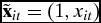
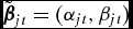
\Pr (y_{ijt} = 1) &\ = \ \Phi (\alpha _{jt} + \beta _{jt} x_{it}) \ = \ \Phi (\tilde{\mathbf {x}}_{it}^\top \tilde{\bm{\beta }}_{jt} ),
\end{eqnarray}$$
where xit
is justice i’s ideal point at time t, and α
jt
and β
jt
represent the item difficulty and item discrimination parameters for roll call j in time t, respectively. Note that as before we use a vector notation
 $\tilde{\mathbf {x}}_{it} = (1, x_{it})$
and
 $\tilde{\bm{\beta }}_{jt} = (\alpha _{jt}, \beta _{jt})$
. As before, the model can be rewritten with the latent propensity y*
ijt
,
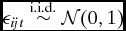
 $$\begin{eqnarray}
y^\ast _{ijt} \ = \ \tilde{\mathbf {x}}_{it}^\top \tilde{\bm{\beta }}_{jt} + \epsilon _{ijt},
\end{eqnarray}$$
where
 $\epsilon _{ijt} \stackrel{\rm i.i.d.}{\sim }\mathcal {N}(0,1)$
and yijt
= 1 (yijt
= 0) if y*
ijt
> 0 (y*
ijt
⩽ 0).
As done in the standard dynamic linear modeling framework, the dynamic aspect of the ideal point estimation is specified through the following random walk prior for each legislator i:
 $$\begin{eqnarray}
x_{it} \mid x_{i,t-1} & \stackrel{\rm indep.}{\sim }& \mathcal {N}(x_{i,t-1},\ \omega _x^2)
\end{eqnarray}$$
for
 $t = \underline{T}_i,\underline{T}_i + 1,\dots ,\overline{T}_i - 1,\overline{T}_i$
where
 $\underline{T}_i$
is the first time period legislator i enters the data and
 $\overline{T}_i$
is the last time period the legislator appears in the data, i.e.,
 $1 \le \underline{T}_i \le \overline{T}_i \le T$
. In addition, we assume
 $x_{i,\underline{T}_i - 1} \stackrel{\rm i.i.d.}{\sim }\mathcal {N}(\mu _{x}, \Sigma _{x})$
for each legislator i.
Finally, given this setup, with the independent conjugate prior on
 $\tilde{\bm{\beta }}_{jt}$
, we have the following joint posterior distribution:
 $$\begin{eqnarray}
p(\mathbf {Y}^\ast ,\lbrace \mathbf {x}_{i}\rbrace _{i=1}^N, \lbrace \tilde{\bm{\beta }}_j\rbrace _{t=1}^T \mid \mathbf {Y}) \nonumber \\
\quad\propto \prod _{i=1}^N \prod _{t = \underline{T}_i}^{\overline{T}_i} \prod _{j=1}^{J_t} \left( \mathbf {1}\lbrace y_{ijt}^\ast > 0\rbrace \mathbf {1}\lbrace y_{ijt} = 1\rbrace\right.\nonumber\\
\qquad\left.\,+\, \mathbf {1}\lbrace y_{ijt}^\ast \le 0\rbrace \mathbf {1}\lbrace y_{ijt} = 0\rbrace \right)\ \phi _1\left(y_{ijt}^\ast ; \tilde{\mathbf {x}}_{it}^\top \tilde{\bm{\beta }}_{jt}, 1\right) \nonumber \\
\qquad\times \prod _{i=1}^N \left\lbrace \phi _1(x_{i,\underline{T}_i-1}; \mu _x, \Sigma _x) \prod _{t=\underline{T}_i}^{\overline{T}_i} \phi _1(x_{it}; x_{i,t-1}, \omega _x^2)\right\rbrace\nonumber\\
\qquad\,\times\,\prod _{t=1}^T \prod _{j=1}^{J_t} \phi _2(\tilde{\bm{\beta }}_{jt}; \bm{\mu }_{\tilde{\bm{\beta }}}, \bm{\Sigma }_{\tilde{\bm{\beta }}}),
\end{eqnarray}$$
where
 $\mathbf {x}_i = (x_{i\underline{T}_i},\dots ,x_{i\overline{T}_i})$
for i = 1, . . ., N.
We propose a variational EM algorithm for the dynamic ideal point model summarized above. The variational inference makes factorization assumptions and approximates the posterior inference by minimizing the Kullback-Leibler divergence between the true posterior distribution and the factorized distribution (see Wainwright and Jordan (Reference Wainwright and Jordan2008) for a review and Grimmer (Reference Grimmer2011) for an introductory article in political science). In the current context, we assume the following factorization assumption:
 $$\begin{eqnarray}
&&q(\mathbf {Y}^\ast , \lbrace \mathbf {x}_{i}\rbrace _{i=1}^N, \lbrace \tilde{\bm{\beta }}_j\rbrace _{t=1}^T)\nonumber\\
&&\quad = \prod _{i=1}^N \prod _{t=\underline{T}_i}^{\overline{T}_i} q(y_{it}^\ast ) \prod _{i=1}^N q(\mathbf {x}_i) \prod _{t=1}^T\prod _{j=1}^{J_t} q(\tilde{\bm{\beta }}_{jt})
\end{eqnarray}$$
which basically assumes the independence across parameters. Importantly, we do not assume the independence between xit and x it′ so that we do not sacrifice our ability to model dynamics of ideal points. We also do not assume a family of approximating distributions. Rather, our results show that the optimal variational distribution belongs to a certain parametric family. The proposed variational EM algorithm is described in the final section while the detailed derivation is given in Appendix C.Footnote 8
An Empirical Application
We apply the proposed variational EM algorithm for estimating the dynamic ideal point to the voting data from the U.S. Supreme court (from October 1937 to October 2013). The data set includes 5,164 votes on court cases by 45 distinct justices over 77 terms, resulting in the estimation of 697 unique ideal points for all justice-term combinations. The same data set was used to compute the ideal point estimates published as the well-known Martin-Quinn scores at http://mqscores.berkeley.edu/ (July 23, 2014 Release version).
We set the prior parameters using the replication code, which was directly obtained from the authors. In particular, the key random-walk prior variance parameter ω2 x is set to be equal to 0.1 for all justices. Note that this choice differs from the specification in Martin and Quinn (Reference Martin and Quinn2002) where Douglas’ prior variance parameter was set as ω2 x = 0.001 because of his ideological extremity and the small number of cases he heard towards the end of his career. This means that Douglas’s ideal point estimate is fixed at his prior mean of − 3.0, but in the results we report below this constraint is not imposed.
We use the same prior specification and apply the proposed variational EM algorithm as well as the standard MCMC algorithm implemented via the MCMCdynamicIRT1d() function from MCMCpack. For the MCMC algorithm, using the replication code, 1.2 million iterations took just over 5 days of computing time. In contrast, our variational EM algorithm took only four seconds. To obtain a measure of estimation uncertainty, we use the parametric bootstrap approach of Lewis and Poole (Reference Lewis and Poole2004) to create 100 replicates and construct bias-corrected 95% bootstrap confidence intervals. Note that even with this bootstrap procedure, the computation is done within several minutes.
We begin by examining, for each term, the correlation of the resulting estimated ideal points for nine justices between the proposed variational inference algorithm and MCMC algorithm. Figure 8 presents both Pearson’s correlations and Spearman’s rank-order correlations. Overall, the correlations are high, exceeding 95% in most cases. In particular, for many terms, rank-order correlations are equal to unity, indicating that the two algorithms produce justices’ estimated ideal points whose rank order is identical. We note that a significant drop in Pearson correlation between 1960 and 1975 is driven almost entirely by the extreme MCMC estimates of Douglas’ position in these years, which correspond to the final years of his tenure. And yet, even in these years, the rank-order correlations remain high.
Correlation of the Estimated Ideal Points for each Term between the Variational EM and Markov Chain Monte Carlo (MCMC) Algorithms

Figures 9 present time series plots of the estimated ideal points for the 16 justices who served the longest periods of time in our study. Solid lines indicate the variational estimates, while the dashed lines indicate their 95% confidence intervals based on the parametric bootstrap. The grey polygons represent the 95% credible intervals obtained from the MCMC algorithm. For almost all justices, the movement of estimated ideal points over time is similar between the two algorithms. Indeed, for most justices, the correlation between the two sets of estimates is high, often exceeding .95. A notable exception to this is Douglas, where we see his ideal point estimates based on the MCMC algorithm becomes more extreme as time passes. The behavior observed here is consistent with earlier warnings about Douglas’ ideological extremity and the fact that he cast only a small number of votes in the final years of his career (Martin and Quinn Reference Martin and Quinn2002). The correlation across all ideal points between the two sets of estimates increases from 0.93 to 0.96, once we exclude Douglas. Overall, our proposed variational inference algorithm produces the estimates of ideal points that are close to the Martin-Quinn score but with significantly less computing time.
Ideal Point Estimates for 16 Longest-serving Justices based on the Variational Inference (VI) and Markov Chain Monte Carlo (MCMC) Algorithm

Simulation Evidence
We further demonstrate the computational scalability of the proposed variational EM algorithm through a series of simulations. We generate a number of roll call matrices that vary in size. These include roll call matrices that have N = 10 legislators and J = 100 roll calls per session (roughly corresponding to the size of the U.S. Supreme Court), roll-call matrices with N = 100 and J = 500 (roughly corresponding to the size of the U.S. Senate), and roll-call matrices with N = 500 and J = 1,000 (roughly corresponding in size to the U.S. House). We also vary the total number of sessions, ranging from T = 10 to T = 100. Thus, the largest roll-call matrix represents a scenario that all members of the U.S. House vote on 1,000 bills during each of 100 consecutive sessions! As we show next, even in this extreme case, our algorithm runs in about 25 minutes, yielding the estimated ideal points that are close to the true values.
We then apply our variational EM algorithm and record the amount of time needed to estimate the model, as well as correlation between the true and recovered ideal points. In the simulation, all legislators serve throughout all periods, whose ideal points in the first period follow the standard normal distribution. Independence across legislators is assumed as done in the model, and their subsequent ideal points are generated as a random walk with ω2 x = 0.1 for all legislators. Item difficulty and discrimination parameters in all sessions were drawn from uniform ( − 1.5, 1.5) and ( − 5.5, 5.5) distributions respectively. While parallelization of the algorithm is trivial and would further reduce run times, we do not implement it for this calculation. As before, convergence is assumed to be achieved when correlation across all parameters across consecutive iterations is greater than 1 − 10−6.Footnote 9
The left panel of Figure 10 displays the amount of time needed for each simulation, with the total number of sessions T given on the horizontal axis. As a benchmark comparison, MCMC replication code provided by Martin and Quinn (Reference Martin and Quinn2002) took over five days to estimate ideal points for U.S. Supreme Court justices over 77 years (N = 45, T = 77, and J = 5,164). For the scenario with N = 10 legislators and J = 100 roll calls per session, estimation is completed under a minute regardless of the number of sessions. Similarly, for the scenarios with 100 legislators and 500 roll calls per session, computation is completed in a matter of minutes regardless of the number of sessions. Computation only begins to significantly increase with our largest scenario of 500 legislators and 1,000 roll calls per session. But even here, for 100 sessions, the variational EM algorithm converges in under 25 minutes.
Scalability and Accuracy of the Proposed Variational Inference for the Dynamic Ideal Point Model

The right panel of the figure presents, for each simulation scenario, the correlation between the variational estimates of ideal points and their true values across all legislators and sessions. The plot demonstrates that the correlation exceeds .95 throughout all the simulations except the case where the size of roll call matrix is small. Even in this case, the correlation is about .90, which suggests the reasonable accuracy of the variational estimates under the dynamic ideal point model.
HIERARCHICAL IDEAL POINT MODEL
Finally, we consider the hierarchical ideal point model where the ideal points are modeled as a linear function of covariates (Bafumi et al. Reference Bafumi, Gelman, Park and Kaplan2005). Like the dynamic ideal point model, there is no closed-form EM algorithm that directly maximizes the posterior distribution. Therefore, we apply variational inference to approximate the posterior distribution. We derive the variational EM algorithm and demonstrate its computational efficiency and the accuracy of approximation through empirical and simulation studies.
The Model
Let each distinct vote be denoted by the binary random variable yl where there exist a total of L such votes, i.e., ℓ ∈ {1, . . ., L}. Each vote y ℓ represents a vote cast by legislator i[ℓ] on bill j[ℓ] (y ℓ = 1 and y ℓ = 0 representing “yea” and “nay,” respectively) where i[ℓ] ∈ {1, . . ., N} and j[ℓ] ∈ {1, . . ., J}. Thus, there are a total of N legislators and J bills. Finally, let g[i[ℓ]] represent the group membership of legislator i[ℓ] where g[i[ℓ]] ∈ {1, . . ., G} and G indicates the total number of groups.
The hierarchical model we consider has the following latent variable structure with the observed vote written as y ℓ = 1{y*ℓ > 0} as before:
 $$\begin{eqnarray}
y^\ast _{\ell } = \alpha _{j[\ell ]} + \beta _{j[\ell ]} x_{i[\ell ]} + \epsilon _{\ell } \quad {\rm where} \quad \epsilon _{\ell } \, \stackrel{\rm i.i.d.}{\sim }\, \mathcal {N}(0,1),\!\!\!\!\nonumber\\
\end{eqnarray}$$
 $$\begin{eqnarray}
x_{i[\ell ]} = \bm{\gamma }_{g[i[\ell ]]}^\top \mathbf {z}_{i[\ell ]} \,{+}\, \eta _{i[\ell ]} \,{\!\!}{\rm where}{\!\!}\, \eta _{i[\ell ]} \,{\!}\stackrel{\rm indep.}{\sim }\, {\!}\mathcal {N}\left(0, \sigma _{g[i[\ell ]]}^2\right),\!\!\!\!\!\!\!\!\nonumber\\
\end{eqnarray}$$
where γ g[i[ℓ]] is an M-dimensional vector of group-specific coefficients, z i[ℓ] is an M-dimensional vector of legislator-specific covariates, which typically includes one for an intercept, and σ2 g[i[ℓ]] is the group-specific variance.
One important special case of this model is a dynamic ideal point model with a parametric time trend, an approach used to compute DW-NOMINATE scores (Poole and Rosenthal Reference Poole and Rosenthal1997) and adopted by some scholars (e.g., Bailey Reference Bailey2007). In this case, the i[ℓ] represents a legislator session, e.g., John Kerry in 2014, and g[i[ℓ]] indicates the legislator, John Kerry, whereas z i[ℓ] may include the number of sessions since the legislator took office as well as a constant for the intercept term. Then, the ideal points are modeled with a linear time trend. In addition, including the square term will allow one to model ideal points using a quadratic time trend. Note that in this setting the time trend is estimated separately for each legislator.
The model is completed with the following conjugate prior distribution:
 $$\begin{eqnarray}
\tilde{\bm{\beta }}_{j[\ell ]} \stackrel{\rm i.i.d.}{\sim }& \mathcal {N}(\bm{\mu }_{\tilde{\bm{\beta }}},\ \bm{\Sigma }_{\tilde{\bm{\beta }}}),
\end{eqnarray}$$
 $$\begin{eqnarray}
\bm{\gamma }_{g[i[\ell ]]} \stackrel{\rm i.i.d.}{\sim }& \mathcal {N}(\bm{\mu }_{\bm{\gamma }},\ \bm{\Sigma }_{\bm{\gamma }}),
\end{eqnarray}$$
 $$\begin{eqnarray}
\sigma _{g[i[\ell ]]}^2 \stackrel{\rm i.i.d.}{\sim }& \mathcal {IG}\left(\displaystyle\frac{\nu _\sigma }{2}, \frac{s_\sigma ^2}{2} \right),
\end{eqnarray}$$
where
 $\tilde{\bm{\beta }}_{j[\ell ]}=(\alpha _{j[\ell ]},\bm{\beta }_{j[\ell ]})$
and
 $\mathcal {IG}(\nu , s^2)$
represents the inverse-gamma distribution with scale and shape parameters equal to ν and s
2, respectively.
It is convenient to rewrite the model in the following reduced form:
 $$\begin{eqnarray}
y_\ell ^\ast & = & \alpha _{j[\ell ]} + \beta _{j[\ell ]}\bm{\gamma }_{g[i[\ell ]]}^\top \mathbf {z}_{i[\ell ]} + \beta _{j[\ell ]} \eta _{i[\ell ]} + \epsilon _\ell
\end{eqnarray}$$
Then, the joint posterior distribution is given by
 $$\begin{eqnarray}
&& p(\mathbf {Y}^\ast , \lbrace \tilde{\bm{\beta }}_{k}\rbrace _{k=1}^J, \lbrace \bm{\gamma }_m\rbrace _{m=1}^G, \lbrace \eta _n\rbrace _{n=1}^N \mid \mathbf {Y}) \nonumber \\
&&\quad\propto \prod _{\ell =1}^L \prod _{k=1}^J \prod _{n=1}^N \prod _{m=1}^G \left(\mathbf {1}\lbrace y_{ij}^\ast \ge 0, y_{ij} = 1 \rbrace \right. \nonumber \\
&&\left.\quad +\, \mathbf {1}\lbrace y_{ij}^\ast < 0, y_{ij} = 0 \rbrace \right) \nonumber \\
&&\quad\times\,\phi _1(y_{\ell }^\ast ; \alpha _k + \beta _k\bm{\gamma }_m^\top \mathbf {z}_n + \beta _k\eta _n, 1)^{\mathbf {1}\lbrace j[\ell ]=k, i[\ell ]=n, g[i[\ell ]]=m\rbrace } \nonumber \\
&&\quad \times \prod _{k=1}^J \phi _2(\tilde{\bm{\beta }}_k; \bm{\mu }_{\tilde{\bm{\beta }}}, \bm{\Sigma }_{\tilde{\bm{\beta }}}) \prod _{n=1}^N \prod _{m=1}^G \phi _1(\eta _n; 0, \sigma _{m}^2) ^{\mathbf {1}\lbrace g[n]=m\rbrace } \nonumber \\
&&\quad\times\,\prod _{m=1}^G \mathcal {IG}\left(\sigma ^2_m; \frac{\nu _\sigma }{2}, \frac{s_\sigma ^2}{2}\right).
\end{eqnarray}$$
For this hierarchical model, there is no closed-form EM algorithm that can directly maximize the posterior distribution given in equation (39). Therefore, as done in the case of the dynamic model, we seek the variational approximation. The factorization assumption we invoke is given by the following:
 $$\begin{eqnarray}
q\left(\mathbf {Y}^\ast , \lbrace \tilde{\bm{\beta }}_k\rbrace _{k=1}^J, \lbrace \bm{\gamma }_m, \sigma _m^2 \rbrace _{m=1}^G, \lbrace \eta _n\rbrace _{n=1}^N\right) \nonumber \\
\quad= \prod _{\ell =1}^L q(y_\ell ^\ast ) \prod _{k=1}^J q(\tilde{\bm{\beta }}_k) \prod _{m=1}^G q(\bm{\gamma }_m) q(\sigma _m^2) \prod _{n=1}^N q(\eta _n).
\end{eqnarray}$$
Under this factorization assumption, we can derive the variational EM algorithm that approximates the joint posterior distribution by maximizing the lower bound. Note that aside from the factorization assumption no additional assumption is made to derive the proposed algorithm. The proposed algorithm is described in the final section while the derivation is given in Appendix D.
Simulation Evidence
We conduct a simulation study to demonstrate the computational scalability and accuracy of the proposed variational EM algorithm. To do this, we generate roll-call matrices that vary in size following the simulation study for dynamic models where the number of legislators is now replaced by the number of groups G instead. Each group has N different ideal points to be estimated, and three covariates z i[ℓ] are observed for each ideal point, i.e., M = 3. Finally, we construct the simulation such that each group votes on the same set of J bills but within each group different members vote on different subsets of the bills.
The intercepts for ideal points follow another uniform distribution with ( − 1, 1), while item discrimination parameters were both drawn uniformly from ( − 0.2, 0.2). The group-level variance parameters σ2 g[i[ℓ]] were set to 0.01 for all groups. We use diffuse priors for item difficulty and discrimination parameters as well as for group-level coefficients. Specifically, the prior distribution for these parameters is the independent normal distribution with a mean of zero and a standard deviation of five. For group-level variance parameters, we use a semi-informative prior such that they follow the inverse-gamma distribution with ν0 = 2 and s 2 = 0.02.
When compared to the other models considered in this article, we find the hierarchical model to be computationally more demanding. To partially address this issue, we parallelize the algorithm wherever possible and implement this parallelized code using eight cores through OpenMP in this simulation study. We also use a slightly less stringent convergence criteria than in the other cases where we check whether the correlations for bill parameters and group-level coefficients across their consecutive iterations is greater than 1 − 10−3. We find that applying a stricter convergence criteria does not significantly improve the quality of the resulting estimates.
We consider three different sets of simulation scenarios where the number of groups G varies from 10 to 500 and the number of bills (per group) J ranges from 100 to 1,000. Figure 11 shows the results. In the left plot, the vertical axis represents the runtime of our algorithm in hours, while the horizontal axis shows the size of each group N, i.e., the number of ideal points to be estimated per group. Our variational EM algorithm scales well to a large data set. In the largest data set we consider (N = 100, J = 1,000, and G = 500), for example, the proposed algorithm can estimate a hundred thousand ideal points in only about 14 hours.
Scalability and Accuracy of the Proposed Variational Inference for the Hierarchical Ideal Point Model

In the right plot of Figure 11, we plot the correlation between the estimated ideal points and their true values for each simulation scenario.Footnote 10 The quality of estimates appear to depend on the number of groups with the simulations with a larger number of groups yielding almost perfect correlation. When the number of groups is small, however, we find that the correlations are weaker and the results are highly dependent on prior specification. This is a well-known feature of Bayesian hierarchical models (Gelman Reference Gelman2006) and the ideal point models appear to be no exception in this regard.
An Empirical Illustration
As noted earlier, DW-NOMINATE scores adopt a linear time trend model for legislators. A model essentially equivalent to this model can be estimated as a special case of our general hierarchical model, in which the covariate z i[l] is the term served by a particular legislator and the ideal point noise parameter η i[l] is fixed at 0.Footnote 11 We analyze the roll-call data from the 1st–100th U.S. House and show empirically that the proposed variational EM algorithm for this model produces the ideal point estimates essentially similar to DW-NOMINATE scores. We specify the prior parameters as νσ = 108 and s 2 σ = 10−8, which effectively fix the noise parameter as desired, and use the same starting values as those used in DW-NOMINATE. An additional constraint we impose that is consistent with DW-NOMINATE is that legislators who serve less than four terms do not shift ideal points over time.
Our model includes G = 10,474 groups (i.e., legislators) with I = 36,177 different ideal points, estimated using J = 48,381 bills. Estimation of the model using eight threads required just under 5 hours of computing time. This run time could be considerably reduced, for example, by not updating η i[ℓ] and σ−2 m , which are fixed at zero. Figure 12 shows the estimated ideal points from the hierarchical model, plotted against the corresponding DW-NOMINATE estimates. The two sets of ideal points correlate at 0.97, thus validating the ability of the hierarchical model to reproduce DW-NOMINATE’s linear time trend ideal point model.
Correlation between DW-NOMINATE Estimates and the Proposed Hierarchical Ideal Point Estimates for the 1st–110th Congress

IDEAL POINT MODELS FOR TEXTUAL AND NETWORK DATA
In recent years, political scientists began to develop and apply ideal point models to new types of data, going beyond roll call votes and survey data. They include text data (e.g., Kim, Londregan, and Ratkovic Reference Kim, Londregan and Ratkovic2014; Lauderdale and Herzog Reference Lauderdale and Herzog2014; Lowe et al. Reference Lowe, Benoit, Mikhaylov and Laver2011; Slapin and Proksch Reference Slapin and Proksch2008) and network data such as campaign contributions(Bonica Reference Bonica2013; Reference Bonica2014), court citations (Clark and Lauderdale Reference Clark and Lauderdale2010), and social media data (Barberá Reference Barberá2015; Bond and Messing Reference Bond and Messing2015). We expect that the applications of ideal point models to these new types of “big data” will continue to increase over the next few years. In this section, we demonstrate that our approach can be extended to these models. In particular, we consider the popular “Wordfish” model of Slapin and Proksch (Reference Slapin and Proksch2008) for text analysis and an ideal point model commonly used for network data analysis.
Fast Estimation of an Ideal Point Model for Textual Data
Suppose that we have a corpus of K documents, each of which is associated with one of N actors, and there are J unique words possibly after pre-processing the corpus (e.g., stemming). Slapin and Proksch (Reference Slapin and Proksch2008) propose to analyze the (J × K) term-document matrix Y using a variant of ideal point model called the Wordfish model (see also Lowe et al. Reference Lowe, Benoit, Mikhaylov and Laver2011, for a related model). Their substantive application is the analysis of manifestos to estimate ideological positions of political parties.
The Generalized Wordfish Model
The original Wordfish model only allows one document per actor. Here, we generalize this model by enabling multiple documents per actor. Let yjk denote the (j, k) element of the term-document matrix Y, representing the frequency of term j in document k. Then, our generalized Wordfish model is defined as
 $$\begin{eqnarray}
p(y_{jk} \mid \alpha _j, \beta _j, \psi _{k}, x_i) = {Poisson}( \lambda _{jk} ),
\end{eqnarray}$$
 $$\begin{eqnarray}
\lambda _{jk} = \exp (\psi _{k} + \alpha _j + \beta _j x_{i[k]} ),
\end{eqnarray}$$
where
 $\psi _{k}$
represents the degree of verboseness of document k, α
j
is the overall frequency of term j across all documents, β
j
is the discrimination parameter for term k, and finally x
i[k] represents the ideological position of the actor to whom document k belongs.
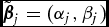
Although the original model is developed under the frequentist framework, we consider the Bayesian formulation by specifying a set of independent prior distributions:
 $$\begin{eqnarray}
p(\tilde{\bm{\beta }}_j) \stackrel{\rm i.i.d.}{\sim }& \mathcal {N}(\bm{\mu }_{\tilde{\bm{\beta }}}, \bm{\Sigma }_{\tilde{\bm{\beta }}}),
\end{eqnarray}$$
 $$\begin{eqnarray}
p(\psi _{k}) \stackrel{\rm i.i.d.}{\sim }& \mathcal {N}(\mu _\psi , \sigma _\psi ^2),
\end{eqnarray}$$
 $$\begin{eqnarray}
p(x_i) \stackrel{\rm i.i.d.}{\sim }& \mathcal {N}(\mu _x, \sigma _x^2),
\end{eqnarray}$$
where
 $\tilde{\bm{\beta }}_j = (\alpha _j, \beta _j)$
is a vector of term parameters. The joint posterior distribution is therefore given by
 $$\begin{eqnarray}
&&p\left(\lbrace \psi _j\rbrace _{k=1}^K, \lbrace \tilde{\bm{\beta }}_j\rbrace _{j=1}^J, \lbrace x_{i=1}^N\rbrace \mid \mathbf {Y}\right) \nonumber\\
&&\quad \propto \left[\prod _{j=1}^J \left\lbrace \prod _{k=1}^K p(y_{jk} \mid \psi _{k}, \tilde{\bm{\beta }}_j, x_{i[k]}) p(\psi _{k})\right\rbrace p(\tilde{\bm{\beta }}_j) \right] \nonumber\\
&&\quad\times\,\prod _{i=1}^N p(x_i).
\end{eqnarray}$$
In Appendix E, we derive the EM algorithm for the local variational inference under the following factorization assumption:
 $$\begin{eqnarray}
&&q\left(\lbrace \psi _{k}\rbrace _{k=1}^K, \lbrace \tilde{\bm{\beta }}_j\rbrace _{j=1}^J, \lbrace x_{i=1}^N\rbrace \right) \nonumber\\
&&\quad = \prod _{j=1}^J q(\tilde{\bm{\beta }}_j) \prod _{k=1}^K q(\psi _{k}) \prod _{i=1}^N q(x_i).
\end{eqnarray}$$
A Simulation Study
We conduct a simulation study to demonstrate the computational scalability and accuracy of the proposed variational EM algorithm. Here, we generate text-document matrices that vary in size. We consider three different sets of simulation scenarios where the number of actors N varies from 100 to 1,000, while the number of words are fixed at J = 5,000. We also vary the number of documents linked to each legislator, K/N, from 10 to 100. Therefore, in this simulation study, the total number of documents, K, ranges from 1,000 to 100,000. Note that the number of parameters to be estimated in this simulation (K + 2J + N) varies from 11,100 to 111,000. Results are shown in Figure 13, with run times on the vertical axis in minutes. In the largest data set we consider (N = 1,000, J = 5,000, K/N = 100), the proposed algorithm completes estimation in under 2.5 hours. For all simulations above, the correlation between the estimated ideal points and their true values exceeds 0.99.
Scalability of the Proposed Variational Inference for the Generalized Wordfish Model

Fast Estimation of an Ideal Point Model for Network Data
We next consider the estimation of ideal points from the network data including citation, social media, and campaign contribution data. These data provide the information about a set of nodes and edges. For example, in the court citation data (Clark and Lauderdale Reference Clark and Lauderdale2010), a node represents a court opinion and the existence of a directed edge from one opinion to another implies a citation. Similarly, in social media data analyzed by Barberá (Reference Barberá2015) and Bond and Messing (Reference Bond and Messing2015), nodes are Twitter and Facebook users and edges indicate whether they follow each other. For campaign contribution data (Bonica Reference Bonica2014), nodes are candidates and voters and edges represent the donations from voters to politicians.
The Network Ideal Point Model
Here, we consider the model developed by Barberá (Reference Barberá2015) to analyze more than four million Twitter users. Let yij = 1{y* ij > 0} represent whether Twitter user i follows politician j where y* ij is the latent propensity where i = 1, 2, . . ., N and j = 1, 2, . . ., J. The network ideal point model is given by
 $$\begin{eqnarray}
y_{ij}^\ast & = & \alpha _j + \beta _i - \Vert x_i - z_j\Vert ^2 + \epsilon _{ij},
\end{eqnarray}$$
where ‖ · ‖ represents the Euclidian norm, and ε ij is the error term.Footnote 12 We assume that ε ij follows the standard normal distribution. The ideal points of Twitter user i and politician j are denoted by xi and zj , respectively. The model assumes that twitter user i are more likely to follow politician j if their ideal points are similar. The model parameters, α j and β i , represents the overall degree to which politician j is followed and Twitter user i follows politicians, respectively.
The model is completed by the following specification of prior distributions:
 $$\begin{eqnarray}
p(\lbrace \alpha _j\rbrace _{j=1}^J) = \prod _{j=1}^{J} \mathcal {N}\left(\mu _\alpha , \sigma _\alpha ^2 \right),
\end{eqnarray}$$
 $$\begin{eqnarray}
p(\lbrace \beta _i\rbrace _{i=1}^N) = \prod _{i=1}^{N} \mathcal {N}\left(\mu _\beta , \sigma _\beta ^2 \right),
\end{eqnarray}$$
 $$\begin{eqnarray}
p(\lbrace x_i\rbrace _{i=1}^N) = \prod _{i=1}^{N} \mathcal {N}\left(\mu _x, \sigma _x^2 \right),
\end{eqnarray}$$
 $$\begin{eqnarray}
p(\lbrace z_j\rbrace _{j=1}^J) = \prod _{j=1}^{J} \mathcal {N}\left(\mu _z, \sigma _z^2 \right).
\end{eqnarray}$$
Together, the joint posterior distribution conditional on the observed (N × J) matrix Y is given by
 $$\begin{eqnarray}
& & p(\mathbf {Y}^\ast , \lbrace \alpha _j\rbrace _{j=1}^J, \lbrace \beta _i\rbrace _{i=1}^N, \lbrace x_i\rbrace _{i=1}^N, \lbrace z_j\rbrace _{j=1}^J \mid \mathbf {Y}) \nonumber \\
&& \quad\propto \prod _{i=1}^N \prod _{j=1}^J \left( \mathbf {1}\lbrace y_{ij}^\ast > 0\rbrace \mathbf {1}\lbrace y_{ij} = 1\rbrace \right.\nonumber\\
&&\left.\quad +\, \mathbf {1}\lbrace y_{ij}^\ast \le 0\rbrace \mathbf {1}\lbrace y_{ij} = 0\rbrace \right)\nonumber\\
&&\quad\times \phi _1\left(y_{ij}^\ast ; \alpha _j + \beta _i - \Vert x_i - z_i\Vert ^2 \right) \nonumber \\
& & \quad\times \prod _{i=1}^{N} \left\lbrace \phi _1 \left(x_i; \mu _{x} , \sigma _{x}^2 \right) \phi _1 \left(\beta _i; \mu _{\beta } , \sigma _{\beta }^2 \right) \right\rbrace \nonumber\\
&&\quad\times\, \prod _{j=1}^{J}\left\lbrace \phi _{1} \left(\alpha _j; \mu _{\alpha } , \sigma _{\alpha }^2 \right) \phi _{1} \left(z_j; \mu _{z} , \sigma _{z}^2 \right) \right\rbrace .
\end{eqnarray}$$
In Appendix F, we derive the variational EM algorithm for the above ideal point model for network data under the following factorization assumption:
 $$\begin{eqnarray}
&&q(\mathbf {Y}^\ast , \lbrace \alpha _j\rbrace _{j=1}^J, \lbrace \beta _i\rbrace _{i=1}^N, \lbrace x_i\rbrace _{i=1}^N, \lbrace z_j\rbrace _{j=1}^J) \nonumber\\
&&\quad = \prod _{i=1}^N \prod _{j=1}^J q(y_{ij}^\ast ) \prod _{i=1}^N q(x_i) q(\beta _i) \prod _{j=1}^J q(\alpha _i) q(z_i). \qquad \end{eqnarray}$$
The variational distributions for the ideal points for users and politicians are based on the second-order Taylor approximation.
An Empirical Study
We test the performance of our estimation algorithm by applying it to a subset of the U.S. Twitter data made available by Barberá (Reference Barberá2015). The original data set includes N = 301,537 voters following J = 318 political elites. Since the replication archive recommends using a subset of N = 10,000 voters following J = 176 political elites, we proceed with this smaller data set instead. Even with this subset of the original data, it took 6.5 days on our machine to sample just 500 posterior draws using an MCMC algorithm via RStan software.Footnote 13 In contrast, our variational EM algorithm was able to complete the estimation for this same data set within 35 minutes even though we did not use any parallelization. This demonstrates the scalability of our algorithm when compared to a standard MCMC algorithm.
In Figure 14, we compare our ideal point estimates with those of Barberá (Reference Barberá2015) for both voters (left panel) and political elites (right panel). In both cases, we observe that the variational EM algorithm produces essentially the same estimates as the Markov chain Monte Carlo algorithm as implemented via RStan software.
Comparison of Our Ideal Point Estimates with Those of Barberá (Reference Barberá2015)

CONCLUDING REMARKS
Political ideology is at the core of political science theories across all subfields. And yet, when conducting empirical analyses, it is impossible to directly observe political ideology. Instead, researchers must infer ideological positions of various actors from their behavior or expressed attitudes. Quantitative analysis of political ideology begins with the specification of a measurement model that formally connects latent ideological positions with observed behavior and attitudes. Over the last couple of decades, ideal point estimation methods based on spatial voting models and item response theory have been the main workhorse for quantitative researchers in political science to measure political ideology. These models have been used to analyze the voting in U.S. Congress (e.g., Poole and Rosenthal Reference Poole and Rosenthal1997), courts (e.g., Martin and Quinn Reference Martin and Quinn2002), other legislatures (e.g., Hix, Noury, and Roland Reference Hix, Noury and Roland2006; Londregan Reference Londregan2007), and United Nations assembly (e.g., Bailey, Strezhnev, and Voeten Reference Bailey, Strezhnev and Voeten2015; Voeten Reference Voeten2000). Beyond roll call votes, the methods are also applied to survey data (e.g., Clinton and Lewis Reference Clinton and Lewis2008), campaign contributions (e.g., Bonica Reference Bonica2014), party manifestos (e.g., Lowe et al. Reference Lowe, Benoit, Mikhaylov and Laver2011), speeches (e.g., Proksch and Slapin Reference Proksch and Slapin2010), and social media (e.g., Bond and Messing Reference Bond and Messing2015).
Over the last decade, political science, like other social science disciplines, witnessed the “big data revolution” where empirical researchers are collecting increasingly large data sets of diverse types. These rich data sets allow researchers to answer the questions they were previously unable to tackle and often enable to employ more realistic but complicated modeling strategies. While the available computational power is steadily increasing, the amount of data available to social scientists and the degree of methodological sophistication are growing at an even faster rate. As a result, researchers are unable to estimate the models of their choice within a reasonable amount of time and are often forced to make a compromise by adopting a feasible and yet undesirable statistical procedure.
In this article, we develop fast estimation algorithms for ideal points with massive data. These algorithms overcome the computational bottleneck created by massive data in the ideal point measurement context. Specifically, we develop the expectation-maximization (EM) algorithms that maximize the posterior distribution. When such an algorithm is not available in a closed form, we derive a variational EM algorithm that approximates posterior inference. Through empirical and simulation studies, we show that the proposed methodology improves the computational efficiency by orders of magnitude without sacrificing the accuracy of the resulting estimates.Footnote 14 With this new methodology, researchers can estimate ideal points from massive data on their laptop within minutes rather than running other estimation algorithms for days on a high-performance computing cluster.
We predict that this line of methodological research will become essential for the next generation of empirical political science research. The political science data now come in a variety of form—textual data, network data, and spatial-temporal data to name a few—and in a large quantity. To efficiently extract useful information from these data will require the development of scalable statistical estimation techniques like the ones proposed in this article.
THE DETAILS OF THE PROPOSED EM ALGORITHMS
In this section, we present the details of the proposed EM algorithms. The derivation of these algorithms is given in the Supplementary Appendix.
The Ordinal Ideal Point Model
Below, we describe the EM algorithm for the three-category ordinal ideal point model. The latent variable updates are equal to
 $$\begin{eqnarray}
{z_{ij}^\ast }^{(t)} = \mathbb {E}\left(z_{ij}^\ast \mid \mathbf {x}_i^{(t-1)}, \tau _j^{(t-1)}, \tilde{\bm{\beta }}_j^{(t-1)}, y_{ij}\right) \nonumber\\
\quad = \left\lbrace \begin{array}{@{}ll@{}}m_{ij}^{(t-1)} -\frac{1}{\tau _j^{(t-1)}}\lambda \left(m_{ij}^{(t-1)},\ \tau _j ^{(t-1)}\right) & \text{if}\ y_{ij}=0,\\
m_{ij}^{(t-1)} + \frac{1}{\tau _j^{(t-1)}}\delta \left(1-m_{ij}^{(t-1)},\ \tau _j^{(t-1)}\right) & \text{if}\ y_{ij}=1,\\
m_{ij}^{(t-1)} + \frac{1}{\tau _j^{(t-1)}}\lambda \left(1-m_{ij}^{(t-1)},\ \tau _j^{(t-1)}\right) & \text{if}\ y_{ij}=2, \end{array}\right. \nonumber\\
\end{eqnarray}$$
where
 $m_{ij}^{(t-1)} = (\tilde{\mathbf {x}}_i^{(t-1)})^\top \tilde{\bm{\beta }}_j^{(t-1)}$
, λ(m, τ) = ϕ(mτ)/{1 − Φ(mτ)} and δ(m, τ) = {ϕ(mτ) − ϕ((1 − m)τ)}/{Φ((1 − m)τ) + Φ(mτ) − 1}. If yij
is missing, then we set z*
ij
(t) = mij
(t − 1). The required second moment is given by
 {\fontsize{6.9}{8.9}\selectfont{$$\begin{eqnarray*}
\left({z_{ij}^\ast }^2\right)^{(t)} = \mathbb {E}({z_{ij}^\ast }^2 \mid \mathbf {x}_i^{(t-1)}, \tau _j^{(t-1)}, \tilde{\bm{\beta }}_j^{(t-1)}, y_{ij}) \nonumber \\
\quad= \left\lbrace \begin{array}{@{}l@{}l@{}}
\left({z_{ij}^\ast }^{(t)}\right)^2 + \frac{1}{\left(\tau _j^{(t-1)}\right)^{2}} \Big[1+\tau _j^{(t-1)}m_{ij}^{(t-1)} \lambda \left(m_{ij}^{(t-1)},\ \tau _j ^{(t-1)}\right) \\[12pt]
\quad - \left\lbrace \lambda \left(m_{ij}^{(t-1)},\ \tau _j ^{(t-1)}\right)\right\rbrace ^2 \Big] & \text{if}\ y_{ij}=0\\[12pt]
\left({z_{ij}^\ast }^{(t)}\right)^2 + \frac{1}{\left(\tau _j^{(t-1)}\right)^{2}} \\[12pt]
\quad\times\, \left[1- \frac{\tau _j^{(t-1)} \left\lbrace m_{ij}^{(t-1)}\phi \left(m_{ij}^{(t-1)} \tau _j ^{(t-1)}\right) + \left(1-m_{ij}^{(t-1)}\right)\phi \left(\left(1-m_{ij}^{(t-1)}\right)\tau _j^{(t-1)}\right)\right\rbrace }{\Phi \left(\left(1-m_{ij}^{(t-1)}\right)\tau _j^{(t-1)}\right) + \Phi \left(m_{ij}^{(t-1)}\tau _j^{(t-1)}\right) - 1}\right.\\[21pt]
\left.\qquad\quad -\, \left\lbrace \delta \left(1-m_{ij}^{(t-1)},\ \tau _j^{(t-1)}\right)\right\rbrace ^2 \right] & \text{if}\ y_{ij}=1\\[12pt]
\left({z_{ij}^\ast }^{(t)}\right)^2 + \frac{1}{\left(\tau _j^{(t-1)}\right)^{2}} \left[1 - m_{ij}^{(t-1)} \lambda \left(1-m_{ij}^{(t-1)},\ \tau _j^{(t-1)}\right)\right. \\[12pt]
\left.\quad\times\,\left\lbrace \lambda \left(1-m_{ij}^{(t-1)},\ \tau _j^{(t-1)}\right) - \left(1-m_{ij}^{(t-1)}\right)\tau _j^{(t-1)} \right\rbrace \right] & \text{if}\ y_{ij}=2 \end{array}\right., \\[-10pt]
\end{eqnarray*}$$}}
where if yij is missing, then we set (z* ij (t))2 = (mij (t − 1))2 + (τ(t − 1) j )−2.
Finally, the M step consists of the following conditional maximization steps:
 $$\begin{eqnarray}
\mathbf {x}_i^{(t)} &=& \left(\bm{\Sigma }_\mathbf {x}^{-1} + \sum _{j=1}^J \left(\tau _j^{(t-1)}\right)^2\bm{\beta }_j^{(t-1)} {\bm{\beta }_j^{(t-1)}}^\top \right)^{-1} \bm{\Sigma }_\mathbf {x}^{-1} \bm{\mu }_\mathbf {x}\nonumber \\
&&+\, \sum _{j=1}^J \left(\tau _j^{(t-1)}\right)^2 \bm{\beta }_j^{(t-1)} ({z_{ij}^\ast }^{(t)} - \alpha _j^{(t-1)}),
\end{eqnarray}$$
 $$\begin{eqnarray}
\tilde{\bm{\beta }}_j^{(t)} &= & \left(\bm{\Sigma }_{\tilde{\bm{\beta }}}^{-1} + \left(\tau _j^{(t-1)}\right)^2 \sum _{i=1}^N \tilde{\mathbf {x}}_i^{(t)} \left(\tilde{\mathbf {x}}_i^{(t)}\right)^\top \right)^{-1} \bm{\Sigma }_{\tilde{\bm{\beta }}}^{-1} \bm{\mu }_{\tilde{\bm{\beta }}}\nonumber \\
&& +\, \left(\tau _j^{(t-1)}\right)^2 \sum _{i=1}^N \tilde{\mathbf {x}}_i^{(t)} {z_{ij}^\ast }^{(t)},
\end{eqnarray}$$
 {\fontsize{6}{8}\selectfont{$$\begin{eqnarray*}
\left(\tau _j^{(t)}\right)^2 \\
&&= \frac{N + \nu _\tau - 2}{s_\tau ^2 + \left(\tilde{\bm{\beta }}_j^{(t)}\right)^\top \left\lbrace \sum _{i=1}^N \tilde{\mathbf {x}}_i^{(t)} \left(\tilde{\mathbf {x}}_i^{(t)}\right)^\top \right\rbrace \tilde{\bm{\beta }}_j^{(t)} - 2 \left(\tilde{\bm{\beta }}_j^{(t)}\right)^\top \sum _{i=1}^N \tilde{\mathbf {x}}_i^{(t)} {z_{ij}^\ast }^{(t)} + \sum _{i=1}^N \left({z_{ij}^\ast }^2\right)^{(t)}}.
\end{eqnarray*}$$}}
The Dynamic Ideal Point Model
The algorithm consists of three steps. First, the latent propensity update step is based on the following optimal approximating distribution:
 $$\begin{eqnarray}
q(y_{ijt}^\ast ) & = & \left\lbrace \begin{array}{@{}ll@{}}\mathcal {TN}\left(m_{ijt}, 1, 0, \infty \right) & \textrm {if}\, y_{ijt} = 1 \\[5pt]
\mathcal {TN}\left(m_{ijt}, 1, -\infty , 0 \right) & \textrm {if}\, y_{ijt} = 0
\end{array}\right.
\end{eqnarray}$$
with
 $m_{ijt}=\mathbb {E}(\tilde{\mathbf {x}}_{it})^\top \mathbb {E}(\tilde{\bm{\beta }}_{jt})$
. Then, the updated mean of y*
ijt
is given by
 $$\begin{eqnarray}
\mathbb {E}(y_{ijt}^\ast ) & = & \left\lbrace \begin{array}{@{}ll@{}}m_{ijt} + \frac{\phi (m_{ijt})}{\Phi (m_{ijt})} & \textrm {if}\, y_{ijt} = 1 \\[5pt]
m_{ijt} - \frac{\phi (m_{ijt})}{1-\Phi (m_{ijt})} & \textrm {if}\, y_{ijt} = 0 \end{array}\right..
\end{eqnarray}$$
For abstention (i.e., missing yijt
), we set
 $q(y_{ijt}^\ast ) = \mathcal {N}(m_{ijt}, 1)$
and
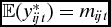 $\mathbb {E}(y_{ijt}^\ast ) = m_{ijt}$
.
Second, the variational distribution for
 $\tilde{\bm{\beta }}$
is given by
 $$\begin{eqnarray}
q(\tilde{\bm{\beta }}_{jt}) & = & \mathcal {N}(\mathbf {B}_{jt}^{-1} \mathbf {b}_{jt}, \ \mathbf {B}_{jt}^{-1}),
\end{eqnarray}$$
where
 $\mathbf {b}_{jt}=\Sigma _{\tilde{\bm{\beta }}}^{-1} \bm{\mu }_{\tilde{\bm{\beta }}} + \sum _{i \in \mathcal {I}_t} \mathbb {E}(\tilde{\mathbf {x}}_{it}) \mathbb {E}(y_{ijt}^\ast )$
and
 $\mathbf {B}_{jt} = \Sigma _{\tilde{\bm{\beta }}}^{-1} + \sum _{i\in \mathcal {I}_t} \mathbb {E}(\tilde{\mathbf {x}}_{it} \tilde{\mathbf {x}}_{it}^\top )$
with
 $\mathcal {I}_t = \lbrace i: \underline{T}_i \le t \le \overline{T}_i\rbrace$
. Note that the summation is taken over
 $\mathcal {I}_t$
, the set of legislators who are present at time t.
Finally, we consider the variational distribution of dynamic ideal points. Here, we rely on the forward-backward algorithm derived for the variational Kalman filtering. Specifically, we first use the forward recursion to compute
 $$\begin{eqnarray}
x_{it} \mid \ddot{y}_{i1},\dots ,\ddot{y}_{it} & \stackrel{\rm indep.}{\sim }& \mathcal {N}(c_{it},\ C_{it}),
\end{eqnarray}$$
where
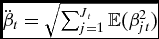 $\ddot{\beta }_{t} = \sqrt{\sum _{j=1}^{J_t} \mathbb {E}(\beta _{jt}^2)}$
,
 $\ddot{y}_{it} \ = \ \lbrace \sum _{j=1}^{J_t} \mathbb {E}(y_{ijt}^\ast ) \mathbb {E}(\beta _{jt}) - \mathbb {E}(\beta _{jt}\alpha _{jt}) \rbrace /\ddot{\beta }_{t}$
,
 $c_{it} = c_{i,t-1} + K_t(\ddot{y}_{it} - \ddot{\beta }_t c_{i,t-1})$
and
 $C_{it} = (1-K_t\ddot{\beta }_t)\Omega _t$
with Ω
t
= ω2
x
+ C
i, t − 1,
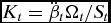 $K_t=\ddot{\beta }_t \Omega _t/S_t$
and
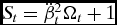 $S_t = \ddot{\beta }_t^2 \Omega _t + 1$
. We recursively compute these quantities by setting c
i0 = μ
x
and C
i0 = Σ
x
. Then, combined with the backward recursion, we can derive the following variational distribution:
 $$\begin{eqnarray}
x_{it} \mid \ddot{y}_{i\underline{T}_i},\dots ,\ddot{y}_{i\overline{T}_i} & \stackrel{\rm indep.}{\sim }& \mathcal {N}(d_{it},\ D_{it}),
\end{eqnarray}$$
where dit
= ct
+ Jt
(d
t + 1 − cit
) and Dit
= Cit
+ J
2
t
(D
t + 1 − Ω
t + 1) with Jt
= Cit
/Ω
t + 1. The recursive computation is done by setting
 $d_{i\overline{T}_i}=c_{i\overline{T}_i}$
and
 $D_{i\overline{T}_i} = C_{i\overline{T}_i}$
. Thus, the required first and second moments of xit
can be easily obtained.
The Hierarchical Ideal Point Model
The proposed EM algorithm cycles through the following updating steps until convergence. First, we update the variational distribution for the latent propensities y*ℓ for all ℓ = 1, . . ., L:
 $$\begin{equation}
q(y_{\ell }^\ast ) \ = \ \left\lbrace \begin{array}{@{}ll@{}}\mathcal {TN}(m_{\ell }, 1, -\infty , 0) & \text{if} \quad y_{\ell }=1\\[4pt]
\mathcal {TN}(m_{\ell }, 1, 0, \infty ,) & \text{if} \quad y_{\ell }=0\\[4pt]
\mathcal {N}(m_{\ell }, 1) & \text{if} \quad y_{\ell } \ \text{is missing }
\end{array}\right.,
\end{equation}$$
where
 $m_\ell = \mathbb {E}(\alpha _{j[\ell ]}) + \mathbb {E}(\beta _{j[l]})\mathbb {E}(\bm{\gamma }_{g[i[\ell ]]})^\top \mathbf {z}_{i[\ell ]} + \mathbb {E}(\eta _{i[\ell ]}) \mathbb {E}(\beta _{j[\ell ]})$
. The required moment update step is given by
 $$\begin{eqnarray}
\mathbb {E}(y_\ell ^\ast ) & = & \left\lbrace \begin{array}{@{}ll@{}}m_\ell + \frac{\phi (m_\ell )}{\Phi (m_\ell )} & {\rm if} \quad y_\ell = 1\\[4pt]
m_\ell - \frac{\phi (m_\ell )}{1-\Phi (m_\ell )} & {\rm if} \quad y_\ell = 0 \\[4pt]
m_\ell & {\rm if} \quad y_\ell {\rm \ is\ missing} \end{array}\right..
\end{eqnarray}$$
Next, we update the first and second moments of the ideal point error term η n using the following variational distribution:
 $$\begin{equation}
q(\eta _n) \ = \ \mathcal {N}(A_n^{-1} a_n,\ A_n^{-1}),
\end{equation}$$
where
 $A_n = \mathbb {E}(\sigma ^{-2}_{g[n]}) + \sum _{\ell =1}^L \mathbf {1}\lbrace i[\ell ] = n\rbrace \mathbb {E}(\beta _{j[\ell ]}^2)$
and
 $a_n=\sum _{\ell =1}^L \mathbf {1}\lbrace i[\ell ] = n \rbrace \lbrace \mathbb {E}(y_\ell ^\ast )\mathbb {E}(\beta _{j[\ell ]}) - \mathbb {E}(\alpha _{j[\ell ]} \beta _{j[\ell ]}) - \mathbb {E}(\beta _{j[\ell ]}^2) \mathbb {E}(\bm{\gamma }_{g[n]})^\top \mathbf {z}_{n}\rbrace$
. Thus, the required moments are given by
 $\mathbb {E}(\eta _n)=A_n^{-1} a_n$
and
 $\mathbb {E}(\eta _n^2)=A_n^{-1} + (A_n^{-1}a_n)^2$
.
Third, we derive the variational distribution for the item parameters. This distribution is equal to
 $$\begin{eqnarray}
q(\tilde{\bm{\beta }}_k) & = & \mathcal {N}(\mathbf {B}_k^{-1}\mathbf {b}_k, \mathbf {B}_k^{-1}),
\end{eqnarray}$$
where
 $\mathbf {B}_k=\bm{\Sigma }_{\tilde{\bm{\beta }}}^{-1} + \sum _{\ell =1}^L \mathbf {1}\lbrace j[\ell ]=k\rbrace \mathbb {E}(\tilde{\mathbf {x}}_{i[\ell ]}\tilde{\mathbf {x}}_{i[\ell ]}^\top )$
and
 $\mathbf {b}_k=\bm{\Sigma }_{\tilde{\bm{\beta }}}^{-1} \bm{\mu }_{\tilde{\bm{\beta }}} + \sum _{\ell =1}^L \mathbf {1}\lbrace j[\ell ]=k\rbrace \mathbb {E}(y_\ell ^\ast ) \mathbb {E}(\tilde{\mathbf {x}}_{i[\ell ]})$
with
 $\tilde{\mathbf {x}}_{i[\ell ]} = (1, \bm{\gamma }_{g[i[\ell ]]}^\top \mathbf {z}_{i[\ell ]}+\eta _{i[\ell ]})^\top$
. We note that
 $\mathbb {E}(\tilde{\mathbf {x}}_{i[\ell ]})=\break (1, \mathbb {E}(\bm{\gamma }_{g[i[\ell ]]})^\top \mathbf {z}_{i[\ell ]}+\mathbb {E}(\eta _{i[\ell ]}))^\top$
and
 $$\begin{eqnarray}
\mathbb {E}\left(\tilde{\mathbf {x}}_{i[\ell ]}\tilde{\mathbf {x}}_{i[\ell ]}^\top \right) \nonumber\\
&& \quad= \left(\begin{array}{cc}
1 & \mathbb {E}(\bm{\gamma }_{g[i[\ell ]]})^\top \mathbf {z}_{i[\ell ]}+\mathbb {E}(\eta _{i[\ell ]}) \\[6pt]
\mathbb {E}(\bm{\gamma }_{g[i[\ell ]]})^\top \mathbf {z}_{i[\ell ]} & \mathbf {z}_{i[\ell ]}^\top \mathbb {E}(\bm{\gamma }_{g[i[\ell ]]}\bm{\gamma }_{g[i[\ell ]]}^\top ) \mathbf {z}_{i[\ell ]}\\[6pt]
+\,\mathbb {E}(\eta _{i[\ell ]})& +\, 2 \mathbb {E}(\bm{\gamma }_{g[i[\ell ]]})^\top \mathbf {z}_{i[\ell ]} \mathbb {E}(\eta _{i[\ell ]})\\[6pt]
& +\, \mathbb {E}(\eta _{i[\ell ]}^2) \end{array} \right). \nonumber\\
\end{eqnarray}$$
This gives the required moment update,
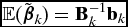 $\mathbb {E}(\tilde{\bm{\beta }}_k)=\mathbf {B}_k^{-1}\mathbf {b}_k$
.
Fourth, the variational distribution for the group-level coefficients is given by
 $$\begin{eqnarray}
q(\bm{\gamma }_m) & = & \mathcal {N}(\mathbf {C}_m^{-1} \mathbf {c}_m,\ \mathbf {C}_m^{-1}),
\end{eqnarray}$$
where
 $\mathbf {C}_m\! =\! \bm{\Sigma }_{\bm{\gamma }}^{-1}\! +\! \sum _{\ell\! =\!1}^L 1\lbrace g[i[\ell ]]\!=\!m\rbrace \mathbb {E}(\beta _{j[\ell ]}^2) \mathbf {z}_{i[\ell ]}\mathbf {z}_{i[\ell ]}^\top$
and
 $\mathbf {c}_m=\bm{\Sigma }_{\bm{\gamma }}^{-1} \bm{\mu }_{\bm{\gamma }} + \sum _{\ell =1}^L 1\lbrace g[i[\ell ]]=m\rbrace \mathbf {z}_{i[\ell ]}[\mathbb {E}(\beta _{j[\ell ]})\break \lbrace \mathbb {E}(y_\ell ^\ast )- \mathbb {E}(\alpha _{j[\ell ]})\rbrace - \mathbb {E}(\beta _{j[\ell ]}^2) \mathbb {E}(\eta _{i[\ell ]})]$
. Thus, the required moment updates are given by
 $\mathbb {E}(\bm{\gamma }_m) = \mathbf {C}_m^{-1}\mathbf {c}_m$
and
 $\mathbb {E}(\bm{\gamma }_m \bm{\gamma }_m^\top )=\mathbf {C}_m^{-1}+\mathbf {C}_m^{-1}\mathbf {c}_m \mathbf {c}_m^\top \mathbf {C}_m^{-1}$
.
Finally, we derive the variational distribution for the group-level variance parameters. This distribution is equal to
 $$\begin{eqnarray}
q(\sigma _m^2) & = & \mathcal {IG}\left(\frac{\nu _\sigma + \sum _{n=1}^N \mathbf {1}\lbrace g[n] = m\rbrace }{2},\ \right.\nonumber\\
&&\left.\times\frac{1}{2} \left(s_\sigma ^2 + \sum _{n=1}^N \mathbf {1}\lbrace g[n] = m\rbrace \mathbb {E}(\eta _n^2)\right) \right),
\end{eqnarray}$$
where the desired moment update is given by
 $\mathbb {E}(\sigma _m^{-2})=[\nu _\sigma +\sum _{n=1}^N \mathbf {1}\lbrace g[n] = m\rbrace ]/[s_\sigma ^2 + \sum _{n=1}^N \mathbf {1}\lbrace g[n] = m\rbrace \mathbb {E}(\eta _n^2)]$
. These updating steps are repeated until convergence.
The Generalized Wordfish Model
The approximate update distribution for the document verboseness parameter
 $\psi _{k}$
for k = 1, . . ., K is given by
 $$\begin{eqnarray}
q(\psi _{k}) &\approx & \mathcal {N}(A_k^{-1} a_k , A_k^{-1})
\end{eqnarray}$$
where
 $a_k = \sum _{j=1}^J [y_{jk} - \exp (\xi _{jk}) \lbrace 1 - \xi _{jk} + \mathbb {E}(\alpha _j) + \mathbb {E}(\beta _j) \mathbb {E}(x_{i[k]})\rbrace ] + \sigma _\psi ^{-2}\mu _\psi$
and Ak
= ∑
J
j = 1exp (ξ
jk
) + σ−2
ψ. Next, the variational distribution for ideal points xn
for n = 1, . . ., N is given by
 $$\begin{eqnarray}
q(x_{n}) & \approx & \mathcal {N}(B_{n}^{-1} b_{n}, B_{n}^{-1}),
\end{eqnarray}$$
where
 $b_{n}= \sum _{j=1}^{J}\sum _{k=1}^{K} \mathbf {1}\lbrace i[k]=n\rbrace \mathbb {E}(\beta _j) \lbrace y_{jk} - \exp (\xi _{jk})(1 + \mathbb {E}(\alpha _j) - \xi _{jk} + \mathbb {E}(\psi _{k}))\rbrace + \sigma _{x}^{-2}\mu _{x}$
and
 $B_{n} =\break \sum _{j=1}^{J}\sum _{k=1}^{K} \mathbf {1}\lbrace i[k]=n\rbrace \exp (-\xi _{jk}) / \mathbb {E}(\beta _j^2) + \sigma _{x}^{-2}$
. Finally, the update for the term parameters
 $\tilde{\bm{\beta }}_j$
for j = 1, . . ., J is given by
 $$\begin{eqnarray}
q(\tilde{\bm{\beta }}_j) & \approx & \mathcal {N}(\mathbf {C}_j^{-1} \mathbf {c}_j , \mathbf {C}_j^{-1}),
\end{eqnarray}$$
where
 $\mathbf {c}_j = \lbrace y_{jk} - \exp (\xi _{jk})(1-\xi _{jk}+\mathbb {E}(\psi _{k})) \rbrace \mathbb {E}(\tilde{\mathbf {x}}_{i[k]}) + \bm{\Sigma }_{\tilde{\bm{\beta }}}^{-1} \bm{\mu }_{\tilde{\bm{\beta }}}$
and
 $\mathbf {C}_j = \sum _{k=1}^K \exp (\xi _{jk}) \mathbb {E}(\tilde{\mathbf {x}}_{i[k]} \tilde{\mathbf {x}}_{i[k]}^\top ) + \bm{\Sigma }_{\tilde{\bm{\beta }}}^{-1}$
.
The Network Ideal Point Model
The variational distribution for the latent propensity is given by the following truncated normal distribution:
 $$\begin{equation}
q(y_{ij}^\ast ) \ = \ \left\lbrace \begin{array}{@{}ll@{}}\mathcal {TN}(m_{ij}, 1, 0, \infty ) & \textrm {if}\, y_{ij} = 1 \\[4pt]
\mathcal {TN}(m_{ij}, 1, -\infty , 0) & \textrm {if}\, y_{ij} = 0
\end{array}\right.,
\end{equation}$$
where
 $m_{ij} = \mathbb {E}(\alpha _j) + \mathbb {E}(\beta _i) - \mathbb {E}(x_i^2) - \mathbb {E}(z_j^2) + 2\mathbb {E}(x_i)\mathbb {E}(z_j)$
.
The variational distribution for the user-specific intercept is given by
 $$\begin{eqnarray}
q(\beta _i) & = & \mathcal {N}(B^{-1} b_i,\ B^{-1}),
\end{eqnarray}$$
where B = J + 1/σ2
β and
 $b_i = \mu _\beta /\sigma _\beta ^2 + \sum _{j=1}^J \left( \mathbb {E}(y_{ij}^\ast ) - \mathbb {E}(\alpha _j) + \mathbb {E}(x_i^2) - 2\mathbb {E}(x_i)\mathbb {E}(z_j) + \mathbb {E}(z_j^2) \right)$
. The update step for the users’ ideal points is based on the following variational distribution:
 $$\begin{eqnarray}
q(\mathbf {x}) & = & \prod _{i=1}^N q(x_i) \ \approx \ \prod _{i=1}^N \mathcal {N}(D_i^{-1} d_i, D_i^{-1}),
\end{eqnarray}$$
where
 $D_i = \mathbb {E}(f^{\prime \prime }(\hat{x}_i))/2$
and
 $d_i = \lbrace \mathbb {E}(f^{\prime \prime }(\hat{x}_i))\hat{x}_i - \mathbb {E}(f^\prime (\hat{x}_i))\rbrace /2$
. The relevant expectations are given by
 $$\begin{eqnarray}
\mathbb {E}(f^\prime (x)) & = & \frac{2}{\sigma _x^2}\left(x - \mu _x\right) \nonumber \\
& & +\, 4\! \sum _{j=1}^J \!\left\lbrace \left(x\,{-}\,\mathbb {E}(z_j)\right)\! \left( \mathbb {E}(y_{ij}^*) \,{-}\, \mathbb {E}(\alpha _j) \,{-}\, \mathbb {E}(\beta _i)\right)\right.\nonumber \\
& &\left. + \left( x^3 - 3 x^2 \mathbb {E}(z_j) + 3 x \mathbb {E}(z_j^2) - \mathbb {E}(z_j^3)\right) \right\rbrace , \nonumber \\
\end{eqnarray}$$
 $$\begin{eqnarray}
\mathbb {E}(f^{\prime \prime }(x)) & = & \frac{2}{\sigma _x^2} + 4\sum _{j=1}^J \left\lbrace \left(\mathbb {E}( y_{ij}^*) - \mathbb {E}(\alpha _j) - \mathbb {E}(\beta _i)\right)\right.\nonumber \\
& &\left. +\, 3 \left(x^2 - 2 x\mathbb {E}( z_j) + \mathbb {E}(z_j^2) \right) \right\rbrace .
\end{eqnarray}$$
The updates for the politician-specific intercept and politicians’ ideal points are similar to the ones for users,
 $$\begin{eqnarray}
q(\alpha _j) = \mathcal {N}(A^{-1} a_j, A^{-1}),
\end{eqnarray}$$
where A = N + 1/σ2
α and
 $a_j = \mu _\alpha /\sigma ^2_\alpha + \sum _{i=1}^N ( \mathbb {E}(y_{ij}^{\ast }) - \mathbb {E}(\beta _i) +(\mathbb {E}(x_i^2) - 2\mathbb {E}(x_i)\mathbb {E}(z_j) + \mathbb {E}(z_j^2) ))$
,
 $$\begin{eqnarray*}
q(z_j) \approx \mathcal {N}(E_j^{-1} e_j, E_j^{-1}),
\end{eqnarray*}$$
where
 $E_j = \mathbb {E}(g^{\prime \prime }(\hat{z}_j))/2$
and
 $e_j = \lbrace \mathbb {E}(g^{\prime \prime }(\hat{z}_j))\hat{z}_j - \mathbb {E}(g^\prime (\hat{z}_j))\rbrace /2$
. The relevant expectations are given by
 $$\begin{eqnarray*}
\mathbb {E}(g^\prime (z)) & = & \frac{2}{\sigma _z^2}\left(z - \mu _z\right) \\
& & - 4 \sum _{i=1}^N \left\lbrace (\mathbb {E}(x_i)-z) \left( \mathbb {E}(y_{ij}^*) - \mathbb {E}(\alpha _j) - \mathbb {E}(\beta _i)\right) \right.\nonumber \\
& &\left.+\, \left( \mathbb {E}(x_i^3) - 3 \mathbb {E}(x_i^2) z + 3 \mathbb {E}(x_i) z^2 - z^3\right) \right\rbrace , \\
\mathbb {E}(g^{\prime \prime }(z)) & = & \frac{2}{\sigma _z^2} + 4\sum _{i=1}^N \left\lbrace \left(\mathbb {E}( y_{ij}^*) - \mathbb {E}(\alpha _j) - \mathbb {E}(\beta _i)\right) \right.\nonumber \\
& &\left.+\, 3 \left(\mathbb {E}(x_i^2) - 2 \mathbb {E}(x_i) z + z^2 \right) \right\rbrace .
\end{eqnarray*}$$
SUPPLEMENTARY MATERIAL
To view supplementary material for this article, please visit https://doi.org/10.1017/S000305541600037X
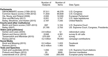
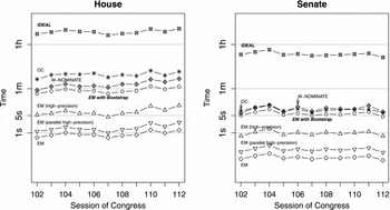
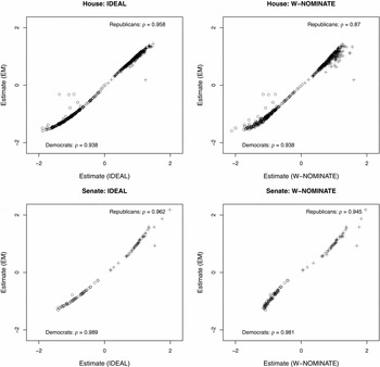
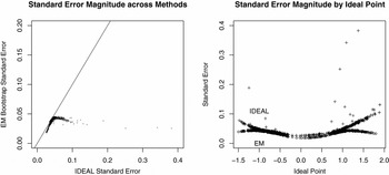
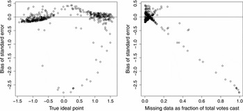
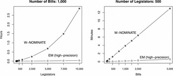
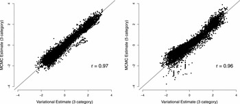
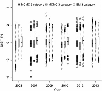
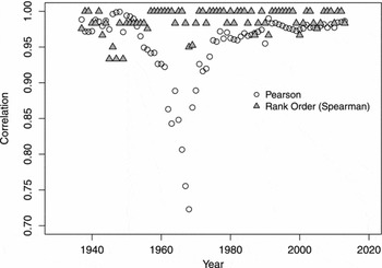
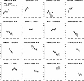
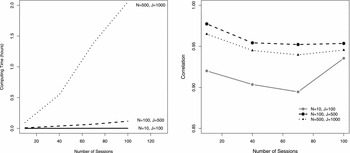
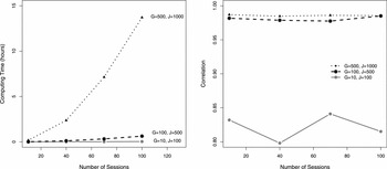
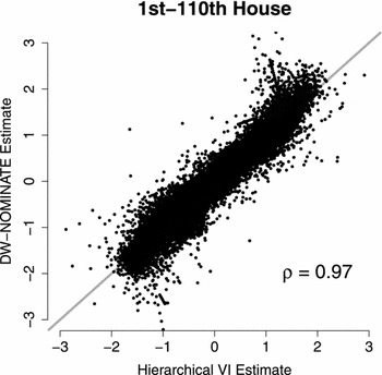
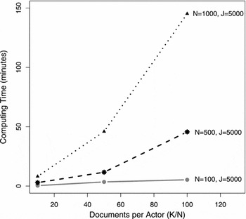
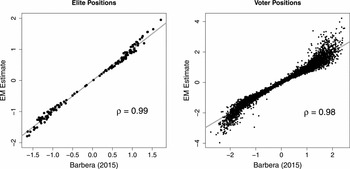




Comments
No Comments have been published for this article.