Nomenclature
-
 $F$
-
generated thrust (N)
-
$h$
-
Inletpressure head (mmWC)
-
$M$
-
total number of bootstrap-trained base models
-
$N$
-
turbine rotational speed (RPM)
-
$n$
-
total number of regressors or trees in ensemble
-
${P_1}$
-
compressor inlet pressure (bar)
-
${P_2}$
-
compressor outlet pressure (bar)
-
${P_3}$
-
combustion chamber pressure (bar)
-
${T_1}$
-
compressor inlet air temperature (°C)
-
${T_2}$
-
fuselage temperature (°C)
-
${T_3}$
-
combustion chamber temperature (°C)
-
${T_4}$
-
turbine exhaust gas temperature (outlet) (°C)
-
${T_5}$
-
nozzle exhaust gas temperature (°C)
-
${T_a}$
-
ambient air temperature (°C)
-
${V_f}$
-
volumetric fuel flow rate (LPH)
-
${w_i}$
-
weight for the
$i$
-th regressor in weighted voting -
$x$
-
input feature vector
-
$\hat y$
-
predicted output (general)
-
${\hat y_{bag}}$
-
ensemble prediction for bagging (N)
-
${\hat y_{{{CatBoost}}}}$
-
ensemble prediction for CatBoost (N)
-
${\hat y_{{{LGBM}}}}$
-
ensemble prediction for LightGBM (N)
-
${\hat y_{stacking}}$
-
ensemble prediction for stacking (N)
-
${\hat y_{{{VR}}}}$
-
ensemble prediction for voting regressor (N)
-
${\alpha _m}$
-
weight for the
$m$
-th learner in AdaBoost -
$\eta $
-
learning rate in CatBoost


Subscripts
- i
-
Index for regressor or feature
- k
-
Index for tree in LightGBM
- m
-
Index for base learner or iteration
1.0 Introduction
The adoption of gas turbine engines (GTEs) in UAV propulsion systems has grown steadily, primarily due to their advantageous power-to-weight characteristics, high operational efficiency and compact design architecture. With UAV platforms increasingly deployed in critical applications such as search and rescue operations, infrastructure assessment, environmental surveillance and aerial monitoring, precise thrust estimation and control have emerged as key requirements for maintaining operational reliability and enhancing overall propulsion performance [Reference Rendón, Sánchez R, Gallo M and A.H.1–Reference Léonard, Borguet and Dewallef3]. The expanding demand for compact, lightweight and high-efficiency propulsion systems for UAVs and model aircraft has accelerated the development of the micro gas turbine industry, thereby stimulating increased research efforts in advanced predictive modelling techniques [Reference Pisano and Lawrence4, Reference Villarreal Valderrama, Takano, Liceaga-Castro, Hernandez-Alcantara, Zambrano-Robledo and Amezquita-Brooks5]. Among the available propulsion configurations, turbojet engines are widely adopted in UAV applications because of their relatively simple mechanical structure and straightforward maintenance requirements [Reference Balli6]. Nevertheless, despite ongoing technological improvements, modelling the transient and nonlinear performance characteristics of gas turbines under varying flight regimes and load conditions remains a complex task. This challenge is particularly evident in small-scale engines, where rapid fluctuations in operating parameters intensify real-time performance variability.
A wide range of data-driven methodologies has been investigated to model the nonlinear and coupled dynamics of gas turbine systems, with particular emphasis on adaptive network-based fuzzy inference systems (ANFIS) and artificial neural networks (ANN). Bartolini et al. [Reference Bartolini, Caresana, Comodi, Pelagalli, Renzi and Vagni7] showed that ANN-based frameworks are capable of accurately representing engine performance across diverse operating regimes, identifying load variation as a more influential factor on power output than parameters such as temperature and pressure. In the context of micro gas turbines (MGTs), Jurado [Reference Jurado8] implemented nonlinear autoregressive models with exogenous inputs (NARX) to analyse system behaviour during electrical disturbances. For off-design performance estimation of single-shaft gas turbines, Lazzaretto and Toffolo [Reference Lazzaretto and Toffolo9] employed feedforward neural networks (FFNN), whereas Ogaji et al. [Reference Ogaji, Singh and Probert10] applied ANN techniques to fault diagnosis in twin-shaft turbine configurations. Arriagada et al. [Reference Arriagada, Genrup, Loberg and Assadi11] utilised multilayer perceptron (MLP) architectures for detecting faults in single-shaft turbines. Mehrpanahi et al. [Reference Mehrpanahi, Hamidavi and Ghorbanifar12] observed that ANN models provide a superior representation of shaft speed dynamics during startup when compared to NARX approaches. Similarly, Basso et al. [Reference Basso, Giarre, Groppi and Zappa13] adopted NARX structures to characterise operational state transitions in heavy-duty gas turbines (HDGTs). Bettocchi et al. [Reference Bettocchi, Pinelli, Spina, Venturini and Burgio14] further validated MLP-based predictive models under varying operating conditions. Bai et al. [Reference Bai, Liu, Chai, Zhao and Yu15] introduced a NARX-driven anomaly detection strategy that demonstrated improved capability in capturing dynamic behaviour relative to conventional techniques. Chiras et al. [Reference Chiras, Evans and Rees16] developed a nonlinear autoregressive moving average model with exogenous inputs (NARMAX) tailored for twin-shaft aero GTEs, integrating both linear and nonlinear dynamic components. Ibrahem et al. [Reference Ibrahem, Akhrif, Moustapha and Staniszewski17] performed a comparative assessment of static and dynamic NARX configurations for triple-shaft aero-derivative turbines and subsequently extended this research [Reference Ibrahem, Akhrif, Moustapha and Staniszewski18] by proposing hybrid ANN–NARX models aimed at enhancing fault detection and condition monitoring. Nikpey et al. [Reference Nikpey, Assadi and Breuhaus19] applied ANN-based methods for health assessment in micro gas turbines, while Vatani et al. [Reference Vatani, Khorasani and Meskin20] combined recurrent neural networks (RNN) with NARX architectures to monitor degradation trends. Tarik et al. [Reference Tarik, Omar, Abdullah and Ibrahim21] implemented NARX modelling specifically for heavy-duty gas turbines operating under low-emission regimes. In addition, Amozegar et al. [Reference Amozegar and Khorasani22] conducted comparative analyses of multiple NARX variants, including RBF-NARX, MLP-NARX and SVM-NARX formulations, whereas Fast et al. [Reference Fast, Palme and Genrup23] integrated ANN approaches with cumulative sum techniques for enhanced monitoring applications.
Recent advancements have further reinforced the prominence of ANN-based methodologies in gas turbine modelling applications. Asgari et al. [Reference Asgari, Chen, Sainudiin, Morini, Pinelli, Spina and Venturini24–Reference Asgari, Chen, Menhaj and Sainudiin26] explored data-driven frameworks for the modelling, simulation and control of GTEs, demonstrating the flexibility and robustness of ANN architectures across diverse operational scenarios. The integration of principal component analysis (PCA) with ANN has also shown considerable promise in enhancing fault detection and diagnostics (FDD) capabilities in industrial gas turbine systems. In a related study, Sarwar et al. [Reference Sarwar, Muhammad, Mokhtar, Khan, Behrani and Kaka27] implemented supervised and unsupervised ANN-based sensor fusion techniques, achieving high diagnostic precision for a twin-shaft 18.7 MW industrial gas turbine. Similarly, Alsarayreh et al. [Reference Alsarayreh, Mohamed and Matar28] examined dual-fuel turbine dynamics using hybrid NARX-ANN and convolutional neural network (CNN) models, reporting that the NARX configuration provided marginally superior performance in predicting shaft speed and exhaust temperature. Despite these advancements, conventional thrust estimation methods in gas turbine engines continue to rely heavily on physics-based thermodynamic cycle analysis, empirical modelling or high-fidelity computational fluid dynamics (CFD) simulations. While such approaches offer valuable physical interpretability, they often depend on simplifying assumptions related to component efficiencies, steady-state approximations and boundary constraints, which may compromise predictive accuracy under highly transient operating conditions. Moreover, the computational expense associated with detailed simulations limits their suitability for real-time applications in small-scale UAV propulsion systems, where rapid thrust prediction is critical for effective control and monitoring. In contrast, data-driven machine learning techniques can capture complex nonlinear relationships directly from experimental data without explicit thermodynamic formulations, enabling rapid inference with lower computational demand. Nevertheless, most prior investigations predominantly employ single neural network structures, which can exhibit drawbacks such as overfitting, sensitivity to training data variability and diminished robustness under rapidly fluctuating operating environments typical of small-scale UAV-based GTEs [Reference Ibrahem, Akhrif, Moustapha and Staniszewski18, Reference Torella, Gamma and Palmesano29].
Given the challenges in accurately representing nonlinear and transient dynamics in gas turbine engines, ensemble methods such as bagging, AdaBoost, LightGBM, CatBoost, stacking and voting remain underexplored for thrust prediction in small-scale UAV applications. Although neural network models dominate the literature, systematic evaluations of modern ensemble regression techniques for real-time thrust estimation under varying experimental conditions are limited. This gap motivates investigating ensemble-based approaches for modelling complex propulsion dynamics.
In response to this need, the present study offers three primary contributions. First, a detailed real-time experimental dataset was obtained from a KingTech K 130G4+ turbojet engine operating under diverse conditions, including variations in rotational speed, fuel flow rate, pressure, temperature and thrust output. Second, several advanced ensemble regression algorithms were implemented and evaluated using standardised preprocessing, training and validation procedures to ensure a consistent and unbiased comparison. Third, the models were systematically examined in terms of predictive accuracy, generalisation performance and robustness to assess their capability in capturing nonlinear thrust behaviour relevant to UAV propulsion systems.
The remainder of this paper is organised as follows. Section 2 describes the experimental configuration and data acquisition methodology. Section 3 presents the ensemble modelling techniques. Section 4 provides the comparative results and performance analysis. Section 5 concludes the study with key findings and outlines potential directions for future work.
2.0 Experimental setup and data collection
A specialised facility has been developed for the performance evaluation of axial-flow gas turbine engines. At the core of this setup is the KingTech K-130G4+ turbojet engine, securely mounted on a custom-designed platform to support detailed performance assessment.
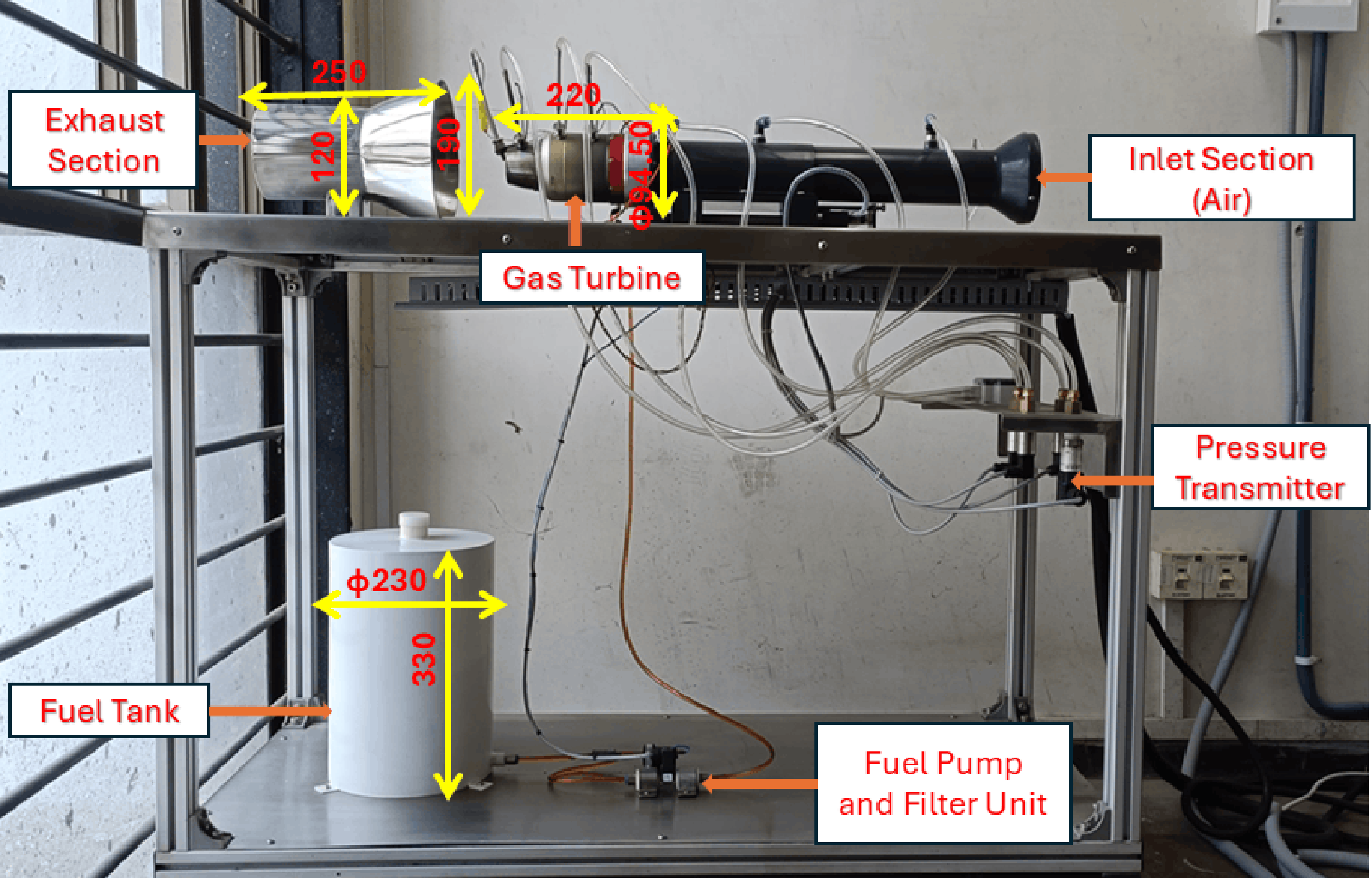
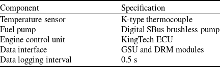
As illustrated in Fig. 1, the system incorporates essential subsystems including a fuel storage and filtration unit, an inlet air management section and a comprehensive instrumentation suite consisting of pressure transducers, thermocouples and an integrated control system. A high-precision data acquisition system operates in real time, continuously capturing critical operating parameters such as thrust, rotational speed, fuel flow rate, temperature distribution and pressure data. The specifications of the instrumentation and data acquisition system used in the experimental setup are summarised in Table 2. The system includes the engine control unit (ECU), temperature sensing devices, fuel delivery components and the associated data interface modules employed for real-time engine monitoring and data logging. This setup enables in-depth analysis of the engine’s dynamic behaviour across a wide range of operating conditions. Key component dimensions are annotated in the Fig. 1. The turbine assembly measures 220 mm in length, with an external casing diameter of 94.5 mm. The exhaust duct extends approximately 250 mm, featuring an inlet diameter of 190 mm and an outlet diameter of 120 mm. The fuel reservoir is 330 mm tall, 230 mm in diameter and has a storage capacity of 15 liters. The inlet and outlet duct sections used in the present experimental setup differ from the original manufacturer configuration and can influence engine performance through changes in airflow and nozzle backpressure. However, fixed duct dimensions were maintained throughout all experiments to ensure consistent operating conditions and reliable comparative analysis for machine learning model development.
Gas turbine experimental setup for thrust measurement and data acquisition.

Figure 1. Long description
A diagram of a gas turbine experimental setup for thrust measurement and data acquisition. The setup includes several labeled components arranged on a metal frame. The inlet section for air is located on the right side, leading into the gas turbine. Following the gas turbine, the exhaust section is positioned on the left side. Below the gas turbine, there is a fuel tank connected to a fuel pump and filter unit. A pressure transmitter is mounted on the frame near the inlet section. Arrows and dimensions indicate the flow and measurements within the system.
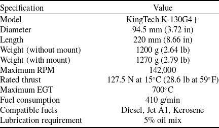
Key specifications of the KingTech K-130G4+ engine are summarised in Table 1, covering geometrical parameters, mass characteristics, operational speed limits, rated thrust, exhaust gas temperature (EGT) thresholds, fuel consumption rate and compatible fuel types.
Technical specifications of the KingTech K-130G4+ turbine engine

Specifications of the instrumentation and data acquisition system

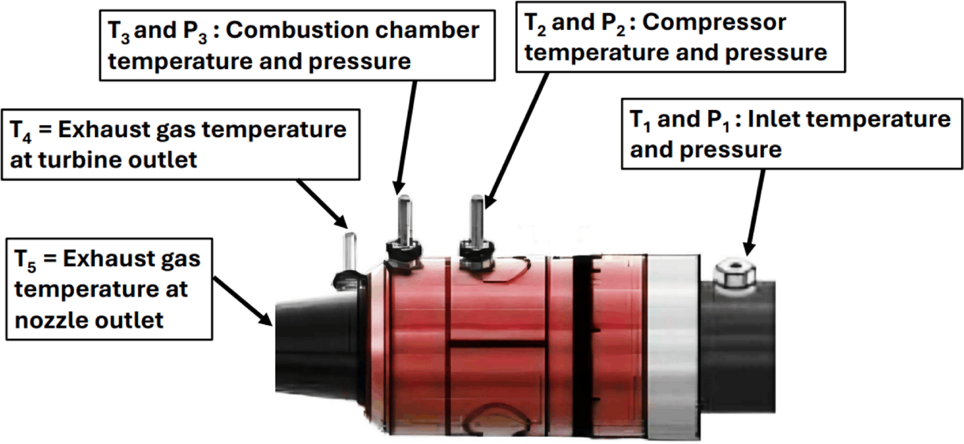
The experimental campaign was conducted over an engine speed range from 40,000 to 90,000 RPM. The experiments were limited to 90,000 RPM to ensure safe and stable operation of the laboratory-scale test setup during repeated steady-state measurements and prolonged data acquisition. Measurements captured included inlet pressure head (
 $h$
) in millimeters of water column (mmWC), fuel flow rate (
 ${V_f}$
) in liters per hour (LPH) and ambient air temperature (
 ${T_a}$
) in degrees Celsius. The parameter
 ${T_a}$
represents the local compressor inlet air temperature measured near the turbojet inlet section under operating conditions, which may vary slightly during engine operation due to localised heating effects and airflow interaction within the experimental setup. Temperature readings (
 ${T_1}$
through
 ${T_5}$
) and pressure measurements (
 ${P_1}$
,
 ${P_2}$
,
 ${P_3}$
) were recorded at strategic locations throughout the engine system, as depicted in Fig. 2. Each operating point was tested multiple times, and average values were used to improve measurement reliability.
Location of temperature and pressure measurements.

The feature variables and target variable employed for machine learning model development are described in the nomenclature section. The selected parameters characterise the thermodynamic and operational state of the engine and are directly related to thrust generation mechanisms. The selection of input features was guided by thermodynamic principles governing turbojet engine operation and the fundamental relationship between thrust generation, mass flow rate, pressure ratio, fuel–air mixing and exhaust gas energy. Turbine rotational speed (
 $N$
) directly influences compressor mass flow rate and overall engine operating point. Fuel flow rate (
 ${V_f}$
) governs combustion energy release and directly affects exhaust gas temperature and thrust output. Inlet pressure head (
 $h$
) and ambient temperature (
 ${T_a}$
) account for variations in inlet air density, which significantly impact mass flow and thrust performance. Temperature measurements (
 ${T_1}$
–
 ${T_5}$
) capture the thermal state of the compressor, combustion chamber and exhaust system, reflecting combustion efficiency and energy transfer through the turbine stages. Pressure variables (
 ${P_2}$
,
 ${P_3}$
) represent compressor and combustion chamber pressure ratios, which are key determinants of engine cycle performance and thrust production. Collectively, these variables represent measurable thermodynamic states that directly influence momentum exchange at the nozzle exit, thereby providing physically meaningful predictors for thrust estimation. The present experimental campaign primarily focused on steady-state operating conditions within the 40,000–90,000 RPM operating range. Although the dataset captures variations in thermodynamic and operational parameters across different engine conditions, it does not fully represent rapid transient throttle transition dynamics and therefore serves as a foundational framework for future dynamic testing studies. The measured temperature and pressure parameters correspond to the principal thermodynamic states of the Brayton cycle across the compressor, combustion chamber, turbine and exhaust sections of the turbojet engine.
Comprehensive safety protocols were implemented during the experimental campaign. Carbon dioxide (CO
 ${_2}$
) fire extinguishers were stationed near the test rig, and flammable materials were cleared from the exhaust vicinity. Operators wore hearing protection and maintained a safe distance from the engine during operation. A post-operation cooling period of 1-2 hours was enforced to avoid residual heat hazards. Electrical systems were carefully regulated between 200 V and 230 V, and all switches were set to OFF before startup.
Pre-startup checks ensured that the ECU was powered by a fully charged battery and that the fuel tank was filled with a properly mixed blend of diesel, Jet A1 or kerosene with 5% oil for lubrication. Fuel lines were purged, brakes were engaged and the model was oriented into the wind before ignition. Engine startup was initiated by setting the GSU throttle trim to activate the ‘Ready’ state, followed by throttle stick cycling. The ECU autonomously managed ignition, preheating, fuel ramping and stabilisation at idle. Shutdown was executed by lowering the throttle trim, triggering a controlled cooling sequence managed by the ECU before safe disconnection of power supplies.
3.0 Ensemble learning methodology
3.1 Bagging
Bagging was introduced in 1996 [Reference Hansen and Salamon30] as an ensemble method aimed at reducing prediction variance and improving generalisation by training multiple base models on resampled datasets obtained through bootstrap sampling. The outputs of these models are then combined, typically by averaging in regression or majority voting in classification tasks [Reference Zhang31]. This technique is especially effective when applied to high-variance learners such as decision trees [Reference Tibshirani and Efron32]. The underlying principle is based on bias–variance decomposition, where the ensemble structure is designed to reduce variance without substantially increasing bias.
The overall ensemble prediction
 ${\hat y_{{\rm{bag}}}}\left( {x{\rm{'}}} \right)$
is obtained by computing the average of the outputs from all base regressors. This aggregation strategy stabilises predictions by reducing sensitivity to fluctuations in the training data. The ensemble prediction is mathematically expressed as Equation (1).
 \begin{align} {\hat y_{{\rm{bag}}}}\!\left( {x{\rm{'}}} \right) = {1 \over M}\mathop \sum \limits_{m = 1}^M {\hat y_m}\left( {x{\rm{'}}} \right) \end{align}
where
 ${\hat y_{{\rm{bag}}}}\left( {x{\rm{'}}} \right)$
denotes the aggregated prediction for input
 $x{\rm{'}}$
,
 $M$
represents the total number of bootstrap-trained base models and
 ${\hat y_m}\left( {x{\rm{'}}} \right)$
corresponds to the prediction generated by the
 ${m^{{\rm{th}}}}$
base regressor.
Algorithm: bagging regression procedure
The implementation procedure of the bagging regression algorithm is summarised as follows:
-
1. Input: Training dataset
$D = \left\{ {\left( {{x_1},{y_1}} \right)\!,\left( {{x_2},{y_2}} \right)\!, \ldots ,\left( {{x_N},{y_N}} \right)} \right\}$
, number of bootstrap iterations
$M$
and base regressor
$h$
. -
2. For
$m = 1$
to
$M$
, generate a bootstrap dataset
${D_m}$
by sampling with replacement from
$D$
. -
3. Train base regressor
${h_m}\!\left( x \right)$
using dataset
${D_m}$
. -
4. For a new input
$x{\rm{'}}$
, compute predictions
${\hat y_m} = {h_m}\!\left( {x{\rm{'}}} \right)$
from each trained model. -
5. Compute the final ensemble prediction using Equation (1).


3.2 AdaBoost
Introduced by Freund and Schapire in 1995 [Reference Freund, Schapire and Abe33], AdaBoost was the first widely recognised boosting technique and remains a foundational method in ensemble learning. In regression applications, AdaBoost combines multiple weak regressors, typically shallow decision trees, in a sequential manner. Each subsequent learner is trained by assigning higher importance to samples with larger prediction errors from previous learners [Reference Freund and Schapire34].
Unlike simple averaging-based ensembles, AdaBoost is adaptive, meaning that the training sample weights are iteratively adjusted based on the performance of preceding models. This sequential reweighting mechanism enables the ensemble to progressively reduce residual errors and improve predictive accuracy.
The final prediction is obtained as a weighted sum of the outputs from all weak learners. The prediction function for AdaBoost regression is expressed as Equation (2).
 \begin{align} \hat y\!\left( x \right) = \mathop \sum \limits_{m = 1}^M {\alpha _m}{h_m}\!\left( x \right) \end{align}
where
 $M$
represents the total number of weak learners,
 ${h_m}\!\left( x \right)$
is the output of the
 ${m^{{\rm{th}}}}$
regressor for input
 $x$
and
 ${\alpha _m}$
denotes the corresponding weight determined according to the weighted regression error of the
 ${m^{{\rm{th}}}}$
learner.
Algorithm: AdaBoost regression procedure
The implementation steps of the AdaBoost regression algorithm are summarised as follows:
-
1. Input: Training dataset
$S = \left\{ {\left( {{x_1},{y_1}} \right)\!,\left( {{x_2},{y_2}} \right)\!, \ldots ,\left( {{x_n},{y_n}} \right)} \right\}$
, number of iterations
$M$
and learning rate
$\eta $
. -
2. Initialise sample weights
${w_{i,1}} = \frac{1}{n}$
for
$i = 1,2, \ldots ,n$
. -
3. For
$m = 1$
to
$M$
, train a weak regressor
${h_m}\!\left( x \right)$
using weighted squared error. -
4. Compute the weighted regression error
${\epsilon _m}$
for the
${m^{{\rm{th}}}}$
learner. -
5. Determine the learner weight
${\alpha _m}$
based on the error
${\epsilon _m}$
. -
6. Update the sample weights by increasing the weights of samples with larger prediction errors.
-
7. Normalise the weights such that
$\mathop \sum \nolimits_{i = 1}^n {w_{i,m + 1}} = 1$
. -
8. Compute the final prediction using Equation (2).


3.3 LightGBM
LightGBM, developed by Microsoft in 2017, is a highly optimised and scalable implementation of gradient boosting that enhances conventional gradient boosting decision tree (GBDT) frameworks [Reference Ke, Meng, Finley, Wang, Chen, Ma, Ye and Liu35]. Compared to traditional GBDT models, LightGBM introduces several innovations to improve computational efficiency and predictive performance. These include a histogram-based algorithm for decision tree construction, a leaf-wise (best-first) growth strategy instead of the conventional level-wise approach, and exclusive feature bundling (EFB) to reduce feature dimensionality. These enhancements enable faster training and better memory utilisation [Reference Ju, Sun, Chen, Zhang, Zhu and Rehman36].
In LightGBM, trees are grown using a leaf-wise strategy, where splits are selected to maximise the reduction in the loss function at each leaf. Unlike depth-wise expansion, this approach captures complex nonlinear relationships more effectively, although it may increase the risk of overfitting if not appropriately regularised. Continuous features are discretised into
 $b$
histogram bins, allowing optimal split selection from these bins and significantly reducing computational cost [Reference Friedman37].
For regression problems, LightGBM builds an additive model in a stage-wise manner. At each iteration, a new tree is fitted to the negative gradients (residuals) of the loss function from the current model. The final prediction is obtained by summing the scaled outputs of all trees, as expressed in Equation (3).
 \begin{align} {\hat y_{{\rm{LGBM}}}}\left( x \right) = {\hat y^{\left( 0 \right)}} + \mathop \sum \limits_{k = 1}^K \eta {h_k}\!\left( x \right) \end{align}
where
 ${\hat y^{\left( 0 \right)}}$
is the initial prediction (typically the mean of the target values),
 $K$
is the total number of trees,
 ${h_k}\!\left( x \right)$
represents the prediction of the
 ${k^{{\rm{th}}}}$
regression tree and
 $\eta $
is the learning rate controlling the contribution of each tree.
Algorithm: LightGBM regression procedure
The LightGBM regression procedure can be summarised as follows:
-
1. Input: Training dataset
$S = \left\{ {\left( {{x_1},{y_1}} \right)\!,\left( {{x_2},{y_2}} \right)\!, \ldots ,\left( {{x_n},{y_n}} \right)} \right\}$
, number of trees
$K$
, number of histogram bins
$b$
, learning rate
$\eta $
and regularisation parameters. -
2. Initialise model prediction
${\hat y^{\left( 0 \right)}}$
(e.g. mean of target values). -
3. For
$k = 1$
to
$K$
:-
(a) Compute gradients (residuals) based on current predictions.
-
(b) Discretise continuous features into
$b$
histogram bins. -
(c) Construct regression tree
${h_k}\!\left( x \right)$
using the binned data. -
(d) Determine optimal splits by minimising the loss function.
-
(e) Expand the tree using the leaf-wise growth strategy.
-
(f) Update the model prediction:
\begin{align*} {\hat y^{\left( k \right)}}\!\left( x \right) = {\hat y^{\left( {k - 1} \right)}}\!\left( x \right) + \eta {h_k}\!\left( x \right) \end{align*}
-
(g) Apply stopping criteria (e.g. maximum depth, minimum leaf samples).
-
-
4. Output final prediction using Equation (3).


3.4 CatBoost
CatBoost, proposed by Dorogush et al. in 2018 [Reference Dorogush, Ershov and Gulin38], is an advanced gradient boosting framework designed to address limitations of conventional boosting methods such as gradient bias and prediction shift [Reference Prokhorenkova, Gusev, Vorobev, Dorogush and Gulin39]. By incorporating ordered boosting and specialised tree construction strategies, CatBoost improves model stability and generalisation performance.
A distinguishing feature of CatBoost is its symmetric (oblivious) tree structure, where the same splitting condition is applied across each level of the tree. This balanced structure reduces variance and enhances computational efficiency. Although CatBoost is particularly well known for its native handling of categorical variables through ordered target encoding, its boosting framework is equally applicable to purely numerical datasets.
For regression tasks, CatBoost builds an additive model in a stage-wise manner, fitting successive trees to the gradients of the loss function. The final prediction is obtained by summing the contributions of all trees as shown in Equation (4).
 \begin{align} {\hat y_{{\rm{CatBoost}}}}\!\left( x \right) = {\hat y^{\left( 0 \right)}} + \mathop \sum \limits_{t = 1}^T \eta {h_t}\!\left( x \right) \end{align}
where
 ${\hat y^{\left( 0 \right)}}$
is the initial prediction (typically the mean of the target variable),
 $T$
denotes the total number of trees,
 ${h_t}\!\left( x \right)$
represents the prediction of the
 ${t^{{\rm{th}}}}$
tree and
 $\eta $
is the learning rate controlling the contribution of each tree.
Algorithm: CatBoost regression procedure
The implementation steps of the CatBoost regression algorithm are summarised as follows:
-
1. Input: Training dataset
$S = \left\{ {\left( {{x_1},{y_1}} \right)\!,\left( {{x_2},{y_2}} \right)\!, \ldots ,\left( {{x_n},{y_n}} \right)} \right\}$
, number of trees
$T$
, learning rate
$\eta $
and regularisation parameters. -
2. Initialise model prediction
${\hat y^{\left( 0 \right)}}$
. -
3. Apply the ordered boosting strategy to the dataset.
-
4. For
$t = 1$
to
$T$
:-
(a) Compute gradients of the regression loss based on current predictions.
-
(b) Construct symmetric (oblivious) tree
${h_t}\!\left( x \right)$
. -
(c) Select optimal splits using gradient-based loss minimisation.
-
(d) Update the model prediction:
\begin{align*} {\hat y^{\left( t \right)}}\!\left( x \right) = {\hat y^{\left( {t - 1} \right)}}\!\left( x \right) + \eta {h_t}\!\left( x \right)\end{align*}
-
-
5. Output final prediction using Equation (4).


3.5 Stacking
Stacking, originally proposed by Smyth and Wolpert in 1997 [Reference Smyth and Wolpert40], is an ensemble learning strategy that integrates multiple base models through a secondary learning algorithm to improve predictive performance. The fundamental idea is to combine diverse base learners by training a meta-learner on their predictions [Reference Ma, Wang, Gao, Wang and Khalighi41].
The stacking framework consists of two levels. In Level-0 (base learners), a set of models
 ${g_1}\!\left( x \right)\!,{g_2}\!\left( x \right), \ldots ,{g_n}\!\left( x \right)$
is trained to generate predictions. In Level-1 (meta-learner), these predictions are used as input features to train a higher-level model
 $h\!\left( \cdot \right)$
that learns how to optimally combine them.
To prevent information leakage and overly optimistic performance estimates, stacking is implemented using out-of-fold (OOF) predictions generated through
 $K$
-fold cross-validation. The final stacking prediction for regression is expressed in Equation (5).
 \begin{align} {\hat y_{{\rm{stacking}}}}\!\left( x \right) = h\!\left( {{g_1}\!\left( x \right)\!,{g_2}\!\left( x \right), \ldots ,{g_n}\!\left( x \right)} \right) \end{align}
where
 ${g_i}\!\left( x \right)$
represents the prediction of the
 ${i^{{\rm{th}}}}$
base learner and
 $h\!\left( \cdot \right)$
denotes the meta-learner responsible for combining the outputs of the base models.
Algorithm: stacking regression procedure
The implementation steps of the stacking regression framework are summarised as follows:
-
1. Input: Training dataset
$S = \left\{ {\left( {{x_1}\!,{y_1}} \right),\left( {{x_2},{y_2}} \right)\!, \ldots ,\left( {{x_m},{y_m}} \right)} \right\}$
, base learners
${g_1},{g_2}, \ldots ,{g_n}$
, meta-learner
$h$
and number of folds
$K$
. -
2. Split the training dataset into
$K$
folds for cross-validation. -
3. For each base learner
${g_i}$
:-
(a) Train
${g_i}$
on
$K - 1$
folds of the training data. -
(b) Predict the outputs for the held-out fold.
-
(c) Store these predictions as OOF predictions.
-
-
4. Construct the meta-feature matrix
${X_{{\rm{meta}}}}$
using the OOF predictions from all base learners. -
5. Train the meta-learner
$h$
using
${X_{{\rm{meta}}}}$
and the corresponding target values. -
6. Retrain all base learners
${g_i}$
on the full training dataset. -
7. For a new input
${x_{{\rm{new}}}}$
, obtain predictions from all base learners and compute the final prediction:
\begin{align*} {\hat y_{{\rm{final}}}} = h\!\left( {{g_1}\left( {{x_{{\rm{new}}}}} \right)\!,{g_2}\!\left( {{x_{{\rm{new}}}}} \right)\!, \ldots ,{g_n}\!\left( {{x_{{\rm{new}}}}} \right)} \right)\end{align*}


3.6 Voting
The voting regressor is a simple ensemble strategy inspired by early work on ensemble averaging by Hansen and Salamon (1990) and aggregation approaches such as bagging introduced by Breiman (1996) [Reference Hansen and Salamon30, Reference Breiman42]. Unlike boosting-based methods, voting does not iteratively update model weights based on residual errors; instead, it aggregates predictions from multiple independently trained regression models to improve stability and robustness [Reference Kilimci43].
The voting approach combines predictions using either simple averaging or weighted averaging. In simple averaging, each model contributes equally to the final prediction, which is computed as the arithmetic mean of their outputs. In weighted averaging, different importance weights are assigned to each model according to its predictive capability, typically satisfying
 $\mathop \sum \nolimits_{i = 1}^n {w_i} = 1$
[Reference Brownlee44]. The ensemble prediction is expressed in Equation (6).
 \begin{align} \hat{y}_{\mathrm{VR}}(x) = \left\{ \begin{matrix} \dfrac{1}{n} \sum_{i=1}^n \hat{y}_i(x) \\[7pt] \sum_{i=1}^n w_i \hat{y}_i(x) \end{matrix} \right. \end{align}
where
 ${\hat y_i}\!\left( x \right)$
denotes the prediction of the
 ${i^{{\rm{th}}}}$
regressor,
 ${w_i}$
represents the weight assigned to that model in the weighted scheme and
 $n$
is the total number of base regressors.
Algorithm: voting regressor procedure
The implementation steps of the voting regression framework are summarised as follows:
-
1. Input: Training dataset
$S = \left\{ {\left( {{x_1},{y_1}} \right),\left( {{x_2},{y_2}} \right), \ldots ,\left( {{x_m},{y_m}} \right)} \right\}$
, base regressors
${R_1},{R_2}, \ldots ,{R_n}$
, voting strategy (simple averaging or weighted averaging) and weights
${w_1},{w_2}, \ldots ,{w_n},$
if weighted voting is used. -
2. Train each base regressor
${R_i}$
independently using the training dataset
$S$
. -
3. For a new input sample
${x_{{\rm{new}}}}$
, obtain predictions from all trained regressors:
\begin{align*} {\hat y_i}\!\left( {{x_{{\rm{new}}}}} \right) = {R_i}\!\left( {{x_{{\rm{new}}}}} \right)\end{align*}
-
4. Combine the predictions using the selected voting strategy:
-
• Simple averaging:
\begin{align*} {\hat y_{{\rm{VR}}}}\!\left( {{x_{{\rm{new}}}}} \right) = {1 \over n}\mathop \sum \limits_{i = 1}^n {\hat y_i}\!\left( {{x_{{\rm{new}}}}} \right)\end{align*}
-
• Weighted averaging:
\begin{align*} {\hat y_{{\rm{VR}}}}\!\left( {{x_{{\rm{new}}}}} \right) = \mathop \sum \limits_{i = 1}^n {w_i}{\hat y_i}\!\left( {{x_{{\rm{new}}}}} \right) \end{align*}
-
5. Output the final ensemble prediction
${\hat y_{{\rm{VR}}}}\!\left( {{x_{{\rm{new}}}}} \right)$
.
-
-


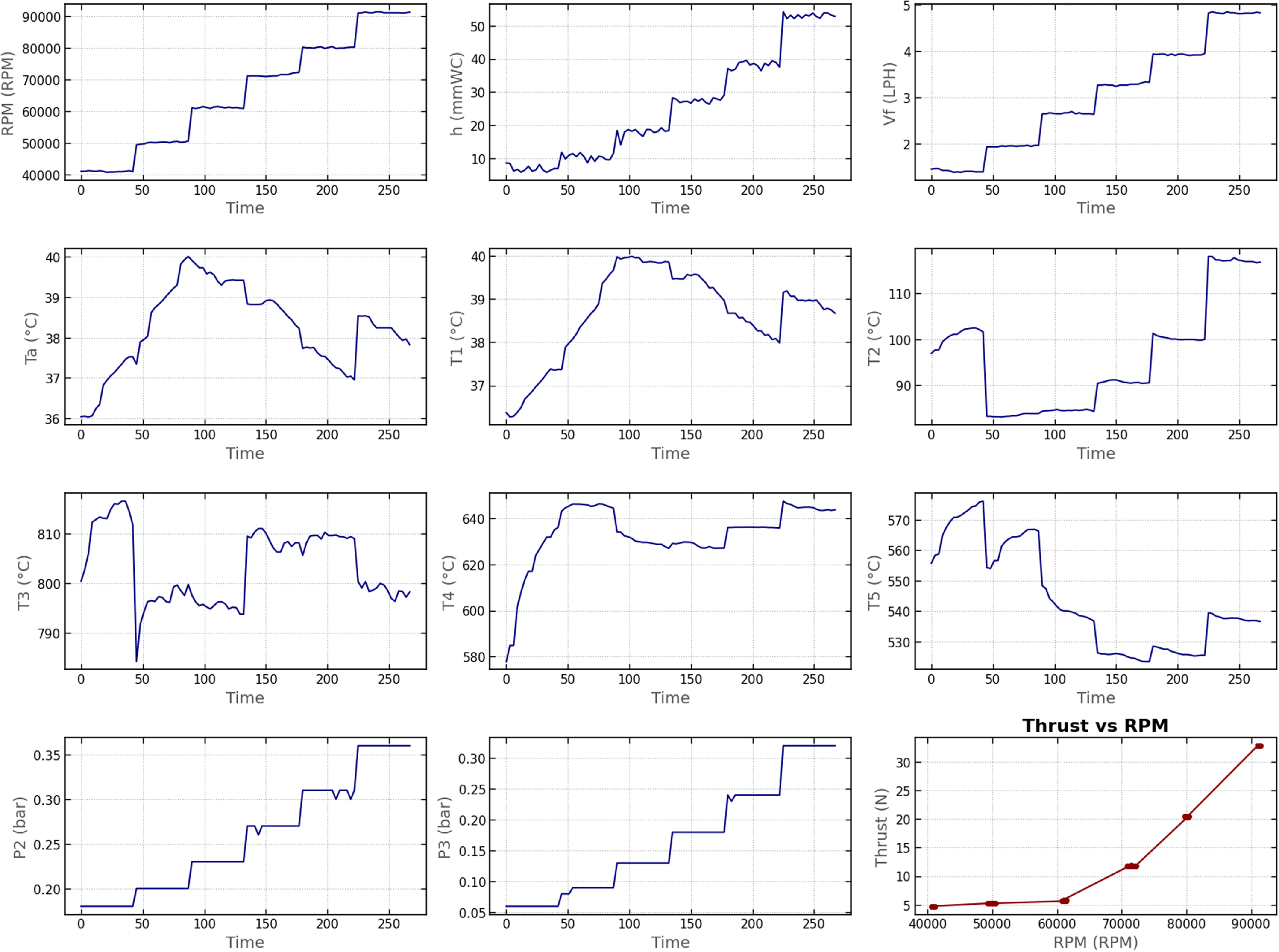
Variation of feature variables and thrust with engine speed (
 $N$
) during gas turbine operation.

Figure 3. Long description
Panel A: A line graph shows the variation of RPM with time. The x-axis is labeled Time and the y-axis is labeled RPM (revolutions per minute). The RPM increases in steps over time. Panel B: A line graph shows the variation of heat input (h) with time. The x-axis is labeled Time and the y-axis is labeled h (millimeters of water column). The heat input increases in steps over time. Panel C: A line graph shows the variation of fuel flow (Vf) with time. The x-axis is labeled Time and the y-axis is labeled Vf (liters per hour). The fuel flow increases in steps over time. Panel D: A line graph shows the variation of ambient temperature (Ta) with time. The x-axis is labeled Time and the y-axis is labeled Ta (degrees Celsius). The ambient temperature shows a peak and then decreases. Panel E: A line graph shows the variation of turbine inlet temperature (T1) with time. The x-axis is labeled Time and the y-axis is labeled T1 (degrees Celsius). The turbine inlet temperature increases and then decreases. Panel F: A line graph shows the variation of turbine exit temperature (T2) with time. The x-axis is labeled Time and the y-axis is labeled T2 (degrees Celsius). The turbine exit temperature shows a peak and then decreases. Panel G: A line graph shows the variation of turbine exit temperature (T3) with time. The x-axis is labeled Time and the y-axis is labeled T3 (degrees Celsius). The turbine exit temperature shows fluctuations over time. Panel H: A line graph shows the variation of turbine exit temperature (T4) with time. The x-axis is labeled Time and the y-axis is labeled T4 (degrees Celsius). The turbine exit temperature increases and then stabilizes. Panel I: A line graph shows the variation of turbine exit temperature (T5) with time. The x-axis is labeled Time and the y-axis is labeled T5 (degrees Celsius). The turbine exit temperature shows fluctuations over time. Panel J: A line graph shows the variation of pressure (P2) with time. The x-axis is labeled Time and the y-axis is labeled P2 (bars). The pressure increases in steps over time. Panel K: A line graph shows the variation of pressure (P3) with time. The x-axis is labeled Time and the y-axis is labeled P3 (bars). The pressure increases in steps over time. Panel L: A scatter plot shows the relationship between thrust and RPM. The x-axis is labeled RPM (revolutions per minute) and the y-axis is labeled Thrust (Newtons). The thrust increases with increasing RPM.
4.0 Results and discussion
The effectiveness of ensemble learning techniques, namely bagging, AdaBoost, LightGBM, CatBoost, stacking and voting, was evaluated for predicting the thrust output of the KingTech K-130G4+ axial-flow GTE. The proposed modelling framework was implemented in a Google Colab environment to ensure computational efficiency and reproducibility. Data processing and numerical computations were performed using pandas and NumPy libraries. Feature standardisation was carried out using StandardScaler from Scikit-learn to normalise input variables prior to model training. The dataset was divided into training and testing subsets using a 60–40 train-test split, with five-fold cross-validation integrated throughout the model development process to ensure robust evaluation and mitigate overfitting. Hyperparameter optimisation was performed using GridSearchCV with five-fold cross-validation to determine optimal configurations for bagging, AdaBoost, LightGBM and CatBoost, incorporating regularisation parameters such as L1/L2 regularisation for LightGBM and l2_leaf_reg for CatBoost to enhance generalisation. The stacking model was configured with internal five-fold cross-validation to prevent data leakage, while the voting regressor combined predictions from multiple base models. Model performance was assessed using MAE, RMSE, coefficient of determination (R2) and cross-validated R² scores (mean ± standard deviation) to provide a comprehensive evaluation of prediction accuracy and model stability.
The predictive framework employed several critical operating variables, including engine rotational speed (
 $N$
in RPM), inlet duct height (
 $h$
in mmWC), fuel flow rate (
 ${V_f}$
in LPH), five temperature measurements (
 ${T_1}$
–
 ${T_5}$
in °C), ambient air temperature (
 ${T_a}$
in °C) and two pressure readings (
 ${P_2}$
and
 ${P_3}$
in bar), as shown in Fig. 3. The thrust force (
 $F$
in N) was modeled as the target variable. The thrust values presented in Fig. 3 correspond to experimentally measured data obtained from the KingTech K-130G4+ gas turbine engine test campaign, while the predictive models were subsequently trained and validated using these experimental measurements. As observed experimentally, thrust exhibits a nonlinear increase with engine speed, reflecting the complex aerodynamic and thermodynamic phenomena within the GTE.
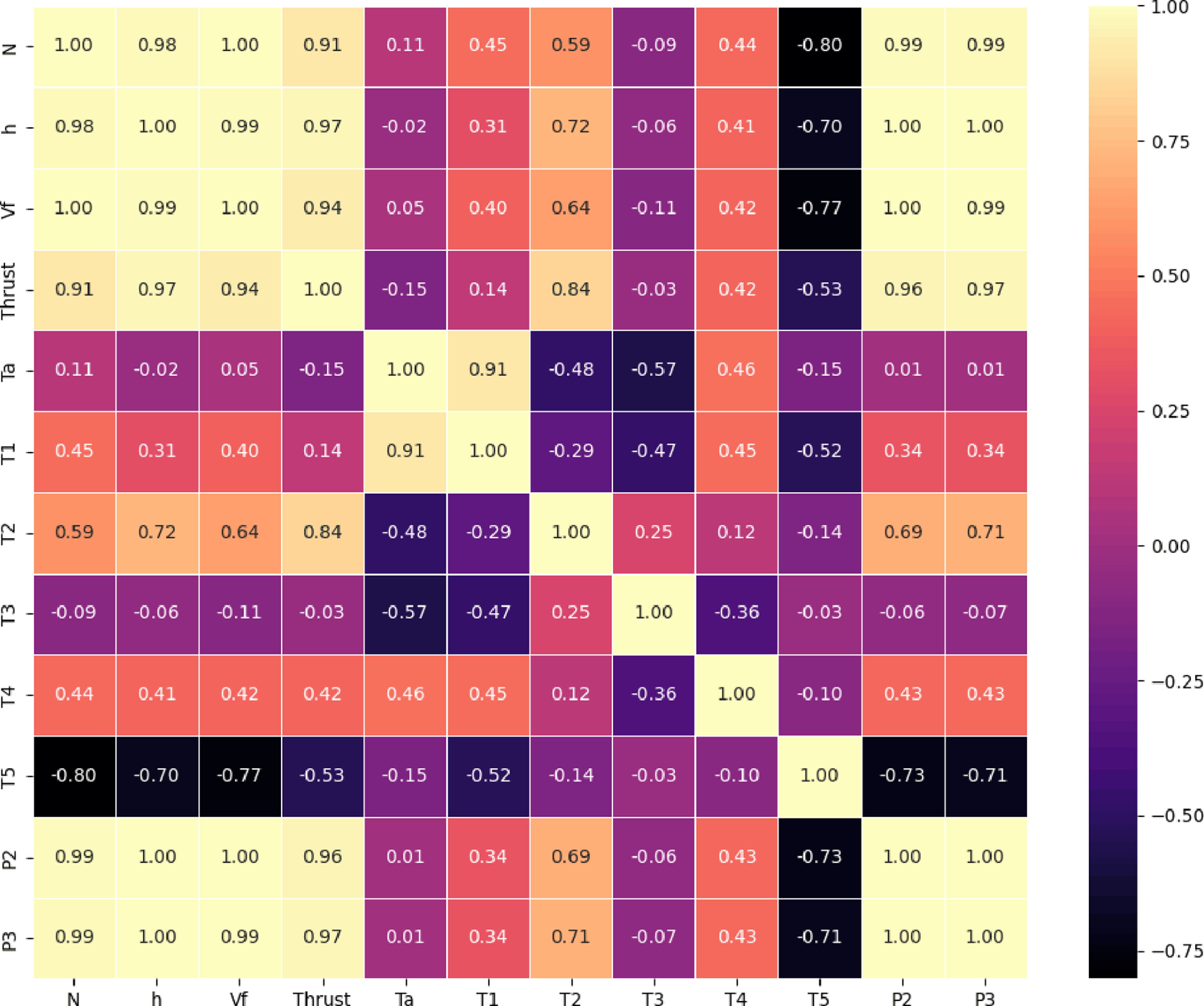
To gain preliminary insights, the correlations with thrust of the features were studied (Fig. 4). The heatmap shows a positive linear correlation of thrust to
 $RPM$
, h,
 ${V_f}$
,
 ${P_2}$
and
 ${P_3}$
suggesting that higher dependence in the output thrust with increasing magnitudes of these operational and pressure-related factors. The temperature-related variables
 $\;{T_2}$
and
 ${T_4}$
are relatively higher (
 $\sim 0.6$
) and of moderate (
 $\sim 0.5$
) level correlation with thrust, respectively. In contrast,
 ${T_5}$
correlates negatively, indicating it is opposed to engine performance. The two other temperature parameters (
 ${T_1}$
and
 ${T_3}$
) present weak to moderate correlations, thus weaker direct linear influence on the thrust production. In conclusion, the correlation analysis indicates that influenced by rotational speed and pressure-related parameters.
Correlation analysis between feature variables and the target variable.

Training set predictions for all ensemble models.

Testing set predictions for all ensemble models.

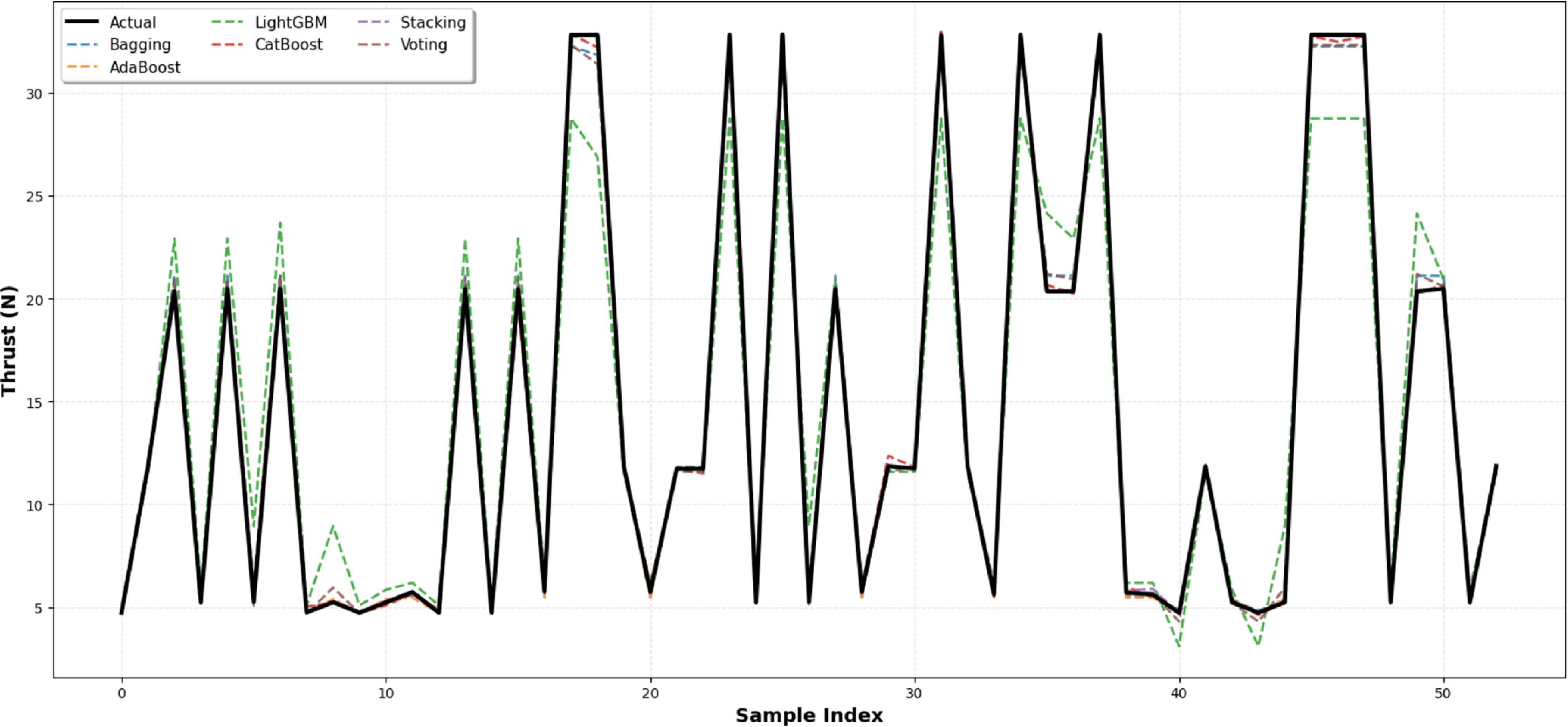
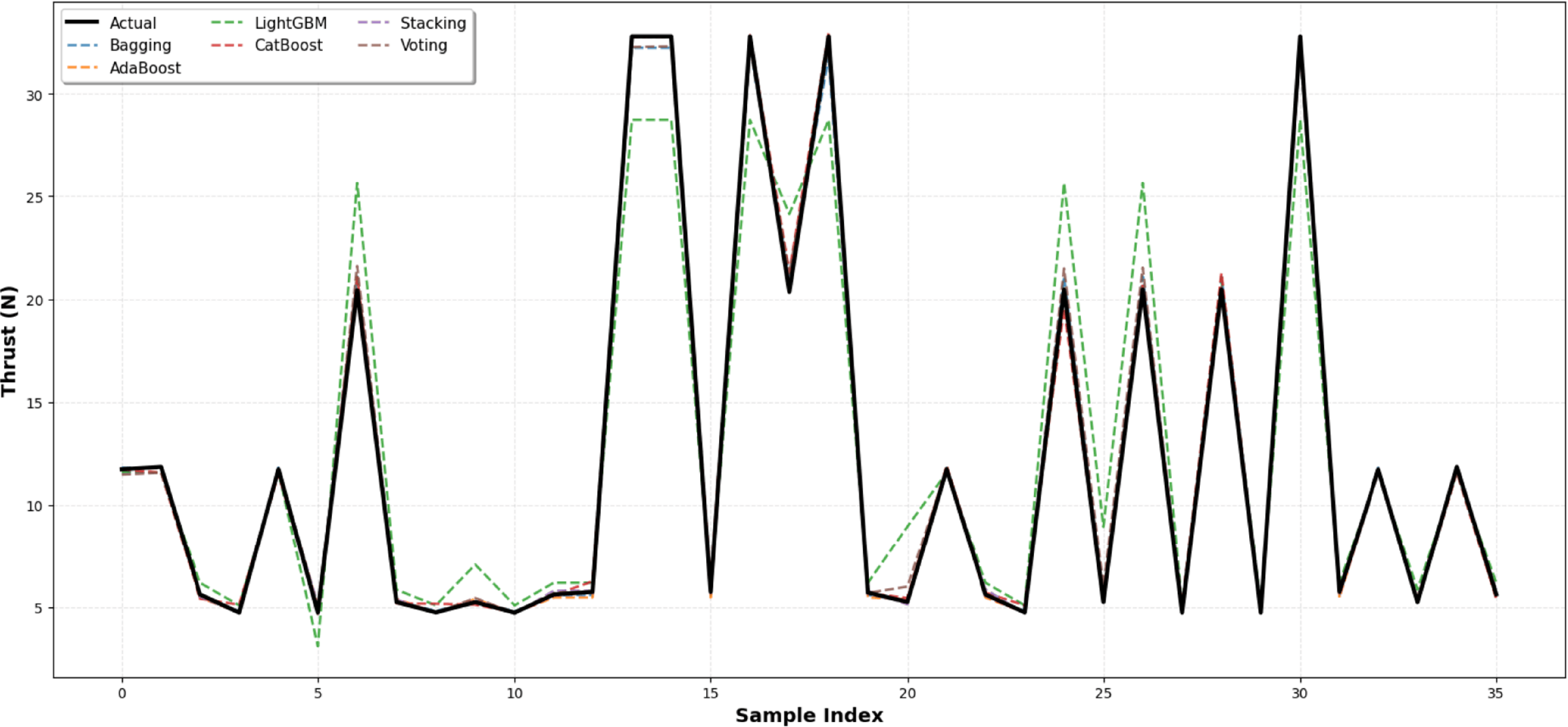
Prior to model development, standard scaling was applied using the StandardScaler from Scikit-Learn to ensure zero mean and unit variance for all input features. The dataset was partitioned into 60% training and 40% testing subsets to balance model learning and generalisation capabilities. This 60–40 split strikes a balance between providing sufficient data for effective model training and ensuring an unbiased assessment of the model’s ability to generalise to new data. After selecting the training and testing data, the hyperparameters of the ensemble regression models were tuned to achieve optimal predictive performance. Grid Search with five-fold cross-validation was employed to systematically explore a predefined set of hyperparameter values for each model. Given the relatively limited dataset size of 90 samples, the adoption of five-fold cross-validation plays an important role in reducing the risk of overfitting and improving the reliability of model evaluation. In this strategy, the dataset is repeatedly partitioned into different training and validation subsets such that each sample contributes to both model training and validation across multiple iterations. This repeated resampling process reduces sensitivity to any single train-test partition and provides a more robust estimate of the model generalisation capability. Furthermore, integrating cross-validation within the hyperparameter optimisation procedure helps prevent the ensemble models from becoming excessively tuned to a specific subset of the experimental data. The training and testing prediction results across all models are presented in Figs 5 and 6, respectively. The relatively broad variation in thrust values corresponds to the complete experimental operating range of the KingTech K-130G4+ engine, including low-throttle and near-maximum RPM conditions within the 40,000–90,000 RPM test envelope. Therefore, the observed thrust distribution reflects the full range of experimentally measured operating states rather than a narrow steady operating condition. All ensemble models demonstrated strong fitting behaviour on the training set, with stacking, AdaBoost and CatBoost showing particularly close agreement with the measured thrust values. On the testing set, stacking achieved the highest predictive accuracy across all operating conditions, followed closely by AdaBoost and CatBoost. Bagging and voting also performed well with stable predictions, while LightGBM exhibited comparatively lower accuracy. These findings indicate that stacking, AdaBoost and CatBoost are the most effective models for thrust prediction in this application.
Residual plots of predicted thrust across all ensemble models.

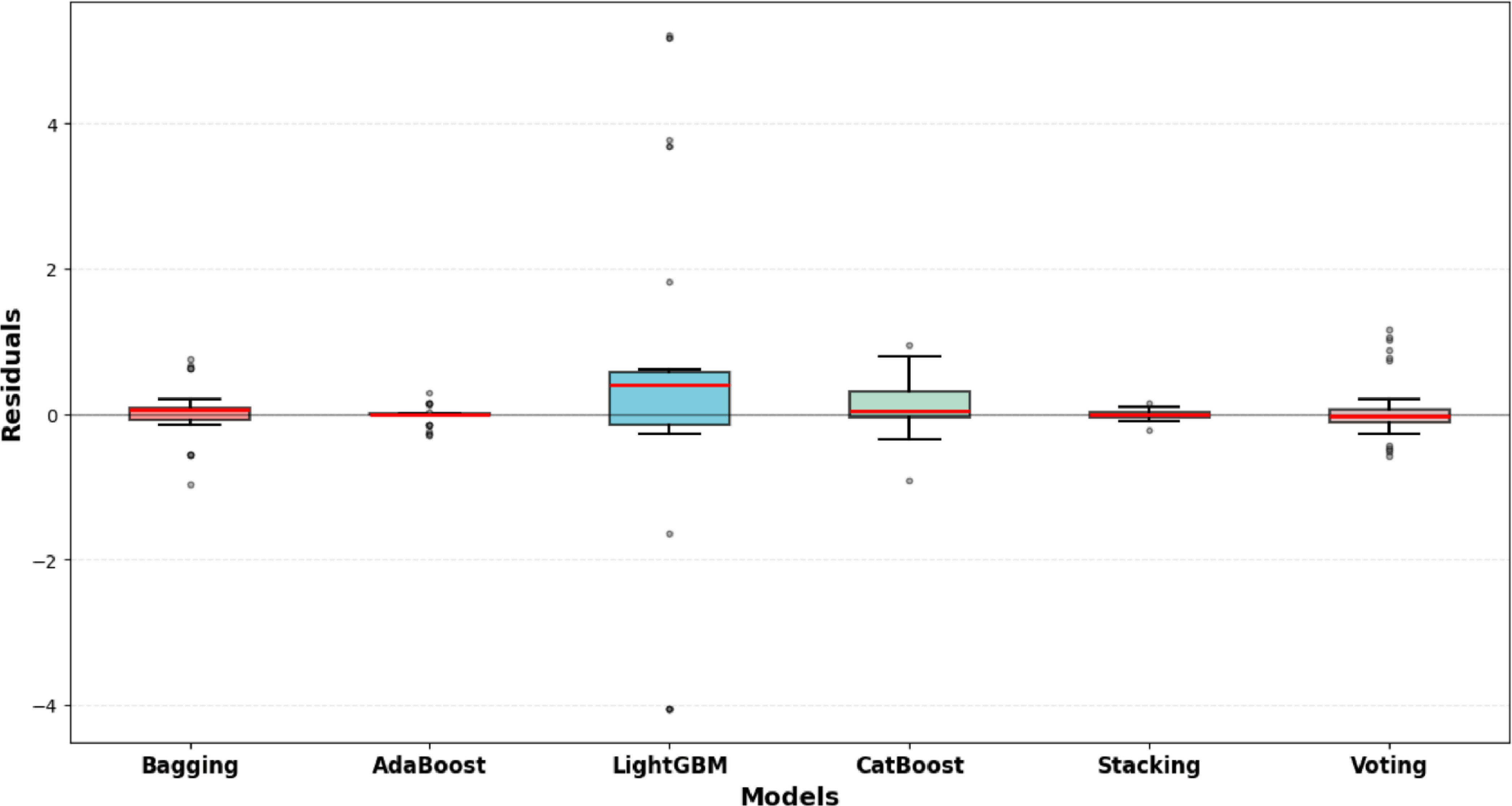
The residual analysis (Fig. 7) provides further insight into the predictive stability and generalisation performance of the evaluated ensemble models. The residuals, defined as the difference between the predicted and experimental thrust values, are largely centred around zero for most models, indicating the absence of significant systematic bias. Stacking exhibits the most compact residual distribution with the narrowest inter-quartile range and minimal extreme values, reflecting exceptional stability and consistent prediction accuracy across all operating conditions. Bagging and voting also demonstrate relatively narrow residual spreads with medians near zero, indicating reliable and consistent performance. AdaBoost and CatBoost show moderate dispersion with residuals centred around zero, suggesting occasional but limited variability. In contrast, LightGBM exhibits the widest residual spread with several extreme outliers, indicating comparatively lower predictive consistency and higher sensitivity to specific data instances. Overall, the differences in residual spread and outlier distribution highlight significant variations in model reliability, with stacking demonstrating the most superior predictive consistency, followed by bagging and voting, while LightGBM shows the highest variability among all evaluated models.
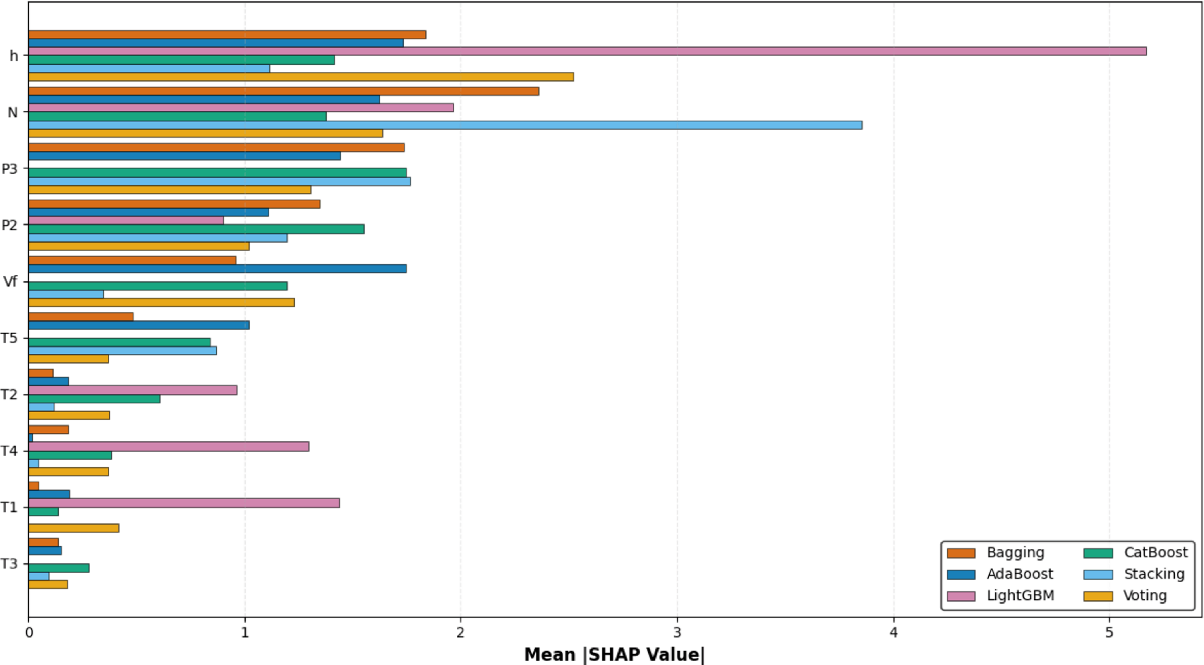
Figure 8 illustrates the comparative feature importance derived from the mean absolute shapley additive explanation (SHAP) values, which quantify the average magnitude of each feature’s contribution to the prediction output across the evaluated models. The mean
 $\left| {{\rm{SHAP}}} \right|$
metric captures the overall influence of a variable on model predictions irrespective of direction, thereby providing a robust measure of global importance. Among the analysed variables,
 $h$
and
 $N$
consistently exhibit the highest contributions across most models, indicating that they are the most influential predictors in determining thrust output. Features such as
 ${P_3}$
,
 ${P_2}$
and
 ${V_f}$
also demonstrate substantial importance, although their relative magnitudes vary across modelling approaches, reflecting differences in how nonlinear relationships and feature interactions are captured. Moderate influence is observed for
 ${T_5}$
,
 ${T_2}$
and
 ${T_4}$
, suggesting that these temperature-related variables contribute meaningfully but not dominantly to predictive performance. In contrast,
 ${T_1}$
and
 ${T_3}$
display comparatively low mean
 $\left| {{\rm{SHAP}}} \right|$
values across all models, indicating a limited marginal impact on the model outputs. Notably, LightGBM shows a distinct feature importance pattern with higher reliance on
 $h$
and
 $N$
compared to other models, while bagging and CatBoost demonstrate more distributed importance across multiple features. Overall, the distribution of SHAP values highlights the dominance of key predictors, particularly
 $h$
and
 $N$
, while also revealing variability in feature sensitivity across models. This emphasises the importance of SHAP-based interpretability for understanding global feature effects in complex predictive systems.
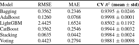
Model performance based on cross-validation metrics

Feature importance analysis using SHAP values across ensemble models.

Figure 8. Long description
Panel A: A horizontal bar graph comparing the mean SHAP values of various input features across different ensemble models. The horizontal axis represents the mean SHAP value, while the vertical axis lists the input features. The input features include h, N, P 3, P 2, V f, T 5, T 2, T 4, T 1, and T 3. The bars are grouped by color, representing different ensemble models: Bagging, CatBoost, AdaBoost, Stacking, LightGBM, and Voting. Notable trends include high mean SHAP values for the input feature h in the LightGBM model and for N in the Stacking model.
The comprehensive model performance comparison is summarised in Table 3. Among all models, stacking demonstrated the highest predictive accuracy with the lowest error metrics (RMSE: 0.0635, MAE: 0.0442) and an exceptional cross-validated R² score of 0.9984 ± 0.0024, indicating excellent generalisation with minimal variance. AdaBoost also exhibited outstanding performance, achieving a near-perfect cross-validated R² of 0.9998 ± 0.0001 with remarkably low RMSE (0.1260) and MAE (0.0768), demonstrating exceptional consistency across cross-validation folds. CatBoost delivered strong results with an R² of 0.9944 ± 0.0032 and RMSE of 0.3562, showing reliable predictive capability. Voting and bagging showed good to moderate performance with R² values of 0.9881 ± 0.0098 and 0.9395 ± 0.0246, respectively. In contrast, LightGBM recorded the highest prediction errors with an RMSE of 2.4425, MAE of 1.6524 and the lowest cross-validated R² of 0.8502 ± 0.1192, along with the highest performance variability, suggesting reduced effectiveness in this particular application.
These findings suggest that ensemble models, particularly stacking, AdaBoost and CatBoost, provide an accurate and robust framework for thrust prediction, offering significant potential for real-time engine health monitoring and autonomous UAV applications. The superior performance of stacking can be attributed to its meta-learning approach that effectively combines the strengths of multiple base estimators, while AdaBoost and CatBoost’s adaptive boosting mechanisms excel at capturing complex nonlinear relationships inherent in gas turbine engine dynamics.
5.0 Conclusion
In this study, ensemble learning-based regression techniques were investigated to model the nonlinear dynamics and parameter interactions governing thrust generation in a gas turbine engine. Six ensemble models, including bagging, AdaBoost, LightGBM, CatBoost, stacking and voting, were trained and evaluated using experimentally acquired data under varying operating conditions. Among the evaluated approaches, the stacking model achieved the lowest prediction errors with RMSE of 0.0635 and MAE of 0.0442, along with a cross-validated R² of 0.9984 ± 0.0024. AdaBoost also demonstrated strong predictive capability, with a cross-validated R² of 0.9998 ± 0.0001 and low associated error metrics. CatBoost delivered consistently high performance with R² of 0.9944 ± 0.0032, while bagging and voting provided moderate to good predictive accuracy. In contrast, LightGBM exhibited comparatively higher error values and larger variability across folds, indicating relatively lower predictive stability within the present dataset.
Overall, the results indicate that ensemble regression techniques, particularly stacking and adaptive boosting methods, can effectively capture the nonlinear relationships between thermodynamic variables and thrust output under the examined experimental conditions. However, it should be noted that the dataset size is limited to 90 samples, and the models were validated within a controlled experimental environment. Therefore, further validation using larger datasets and broader operating conditions is necessary to fully assess the generalisation capability of the proposed models. Nevertheless, the findings demonstrate promising predictive performance for thrust estimation in UAV gas turbine propulsion systems.
From an application perspective, the observed predictive accuracy suggests that ensemble learning approaches may support data-driven thrust estimation frameworks for gas turbine-based UAV propulsion systems. With appropriate validation and implementation considerations, such models could contribute to improved performance monitoring, adaptive control strategies and condition-based maintenance planning. Future work should focus on expanding the dataset, evaluating real-time computational performance and validating the models under flight-representative operating conditions to establish practical deployment feasibility.
Acknowledgements
We gratefully acknowledge the support provided by the Center of Excellence in Aerospace and Defence at the Institute of Infrastructure, Technology, Research, and Management (IITRAM). Access to their advanced facilities and equipment, particularly the KingTech K-130G4+ axial flow gas turbine engine, was essential to the successful execution of this research.
AI use declaration
The authors declare that AI tools were used only for language editing and improving the clarity of the manuscript. All research design, data analysis, results and scientific conclusions are the original work of the authors. The use of AI tools has been transparently declared in accordance with the policies of The Aeronautical Journal and the Royal Aeronautical Society.
 N