Introduction
Measuring and monitoring snow melt is important for studying climate induced changes in polar regions and for hydrological modelling studies of snow melt runoff in high latitude and mountainous regions. The polar regions play an important role in the global heat budget by controlling the exchange of heat, moisture and momentum at the surface–atmosphere interface (Wang Reference Wang2012). At locations with a low surface slope, small changes in surface air temperature can induce large areal changes in wet snow zones on polar ice sheets. Therefore, surface melt of polar ice sheets could serve both as a sensitive indicator and a strong contributing factor to global climate change (Zwally & Fiegles Reference Zwally and Fiegles1994, Liu et al. Reference Liu, Wang and Jezek2005, Reference Liu, Wang and Jezek2006). In high latitude and mountainous regions, snow and glacier ice melt can be a significant contributor to the total yearly runoff volume. Additionally, accurate and timely measurements of the extent of seasonal snow and glacier ice melt are crucial inputs for modelling and forecasting stream discharge, available water resources and possible floods during spring and summer (Ramage & Isacks Reference Ramage and Isacks2003). Although weather stations or shallow snow cores can provide data for snow melt studies, they are often widely scattered. Many empirical studies (Abdalati & Steffen Reference Abdalati and Steffen1995, Reference Abdalati and Steffen1997, Wismann Reference Wismann2000, Joshi et al. Reference Joshi, Merry, Jezek and Bolzan2001, Nghiem et al. Reference Nghiem, Steffen, Kwok and Tsai2001, Bartsch et al. Reference Bartsch, Kidd, Wagner and Bartalis2007) have demonstrated that SSM/I (Special Sensor Microwave Imager) and QuikSCAT (Quick Scatterometer) data are well suited to acquiring temporally detailed records of snow melt. To improve the accuracy of estimating snow melt in the Antarctic, the high spatial resolution of QuikSCAT data and the high reliability of SSM/I data (Lee & Anagnostou Reference Lee and Anagnostou2004, Brown et al. Reference Brown, Derksen and Wang2007, Oza Reference Oza2015) could be combined.
The SSM/I is capable of collecting multifrequency and dual polarization surface radiation measurements, and the QuikSCAT is capable of collecting dual polarization surface scattering measurements. Several scholars have conducted numerous studies on snow melt detection based on SSM/I and QuikSCAT data (Torinesi et al. Reference Torinesi, Fily and Genthon2003, Steffen et al. Reference Steffen, Nghiem, Huff and Neumann2004, Steiner & Tedesco Reference Steiner and Tedesco2014, Bothale et al. Reference Bothale, Rao, Dutt and Dadhwal2015). Regarding the combined use of SSM/I and QuikSCAT data for snow melt detection, there have been a few notable studies. For example, Kunz & Long (Reference Kunz and Long2006) used QuikSCAT data to derive Antarctic snow melt results through the maximum likelihood method and then used SSM/I data for comparison and verification purposes. Ashcraft & Long (Reference Ashcraft and Long2006) proposed a snow melt radiation and scattering physical model for SSM/I data and QuikSCAT data, and used it to obtain information on snow melt in Greenland. Foster et al. (Reference Foster, Hall, Eylander, Riggs, Nghiem, Tedesco, Kim, Montesano, Kelly, Casey and Choudhury2011) derived a global snow product based on optical, SSM/I and QuikSCAT data. Dupont et al. (Reference Dupont, Royer, Langlois, Gressent, Picard, Fily, Cliche and Chum2012) obtained the melt season length of the Barnes ice cap over the 1979–2010 period by using SSM/I and QuikSCAT data. Nghiem et al. (Reference Nghiem, Hall, Mote, Tedesco, Albert, Keegan, Shuman, DiGirolamo and Neumann2012) obtained snow melt information for the Greenland ice sheet by comprehensively analysing the results from optical, SSM/I and QuikSCAT data. The main problem in all the above work is as follows: SSM/I and QuikSCAT data have not been actually combined in terms of the methodology, and the methods used involved separate data processing techniques to obtain corresponding snow melt maps that were then comprehensively analysed and summarized in the results. Therefore, there is a need to further strengthen the methodology for research into snow melt using a synergetic method combining SSM/I and QuikSCAT data.
The aim of this study was to develop a new method to accurately derive snow melt information based on the synergy of SSM/I and QuikSCAT data, i.e. the snow melt physical model directly incorporates the complementary advantages of both types of data. First, attenuation coefficients are calculated for SSM/I and QuikSCAT data for the same positions based on a snow melt physical model. Then, the corrected backscattering coefficients of each pixel point are obtained for QuikSCAT data. With this new method, Antarctic snow melt distribution maps can be created.
Data sets
The SSM/I microwave radiometer data (19.35 GHz vertical polarization (19 V)) were used in this study. SSM/I is mounted on the F8 (9 July 1987 to 30 December 1991), F11 (3 December 1991 to 30 September 1995), F13 (3 May 1995 to 29 April 2009) and F17 (after 1 January 2009) satellite platforms of the Defense Meteorological Satellite Program (DMSP). The DMSP satellites have a near-polar circular sun-synchronous orbit and global coverage over a 24 hour period. The 19.35, 37.05 and 85.50 GHz data have both horizontal and vertical polarization, while the 22.24 GHz data have vertical polarization. The spatial resolution of the 19.35, 22.24 and 37.05 GHz data is 25 km, and the spatial resolution of the 85.50 GHz data is 12.5 km. Microwave radiometers receive thermal radiation from ground-based objects, and this information is primarily used to obtain the surface brightness temperature.
The microwave scatterometer SeaWinds on QuikSCAT (QSCAT) was launched successfully in 1999, and its operating frequency is 13.4 GHz. This system employs a conical scanning pen type antenna. Internal and external beams of QSCAT use two fixed incidence angles (46° and 54°) corresponding to the horizontal polarization (HH) and vertical polarization (VV) modes. This study mainly used the spatial resolution of the SIR (Scatterometer Image Reconstruction) data format (Early & Long Reference Early and Long2001). The format file consists of a header and the data subject, containing the data subject and projection information.
In situ temperature data from Antarctic automatic weather stations (AWSs) include data collected at three hour and ten minute intervals (available free of charge via ftp://amrc.ssec.wisc.edu/). The three hour temperature data are calibrated and some erroneous data removed. The ten minute temperature data are not calibrated and are affected by the acquisition instrumentation and the weather. This study employed three hour temperature data for ground verification purposes, and any unusual data was eliminated based on the daily average data used.
Methods
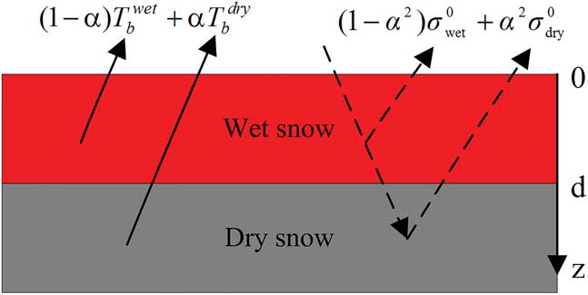
Microwave measurements are very sensitive to the appearance of liquid water in the snow pack. The most significant change in the electromagnetic properties is a large change in the imaginary part of the dielectric constant. The SSM/I microwave radiometer has high reliability and experiences limited effects from roughness, while the microwave scatterometer QuikSCAT has high spatial resolution. There is the same wet snow depth in the same area for the microwave radiometer and scatterometer measurements used in the snow melt physical model (shown in Fig. 1) proposed by Ashcraft & Long (Reference Ashcraft and Long2006). Based on the above model, a synergistic Antarctic snow melt detection method was developed for SSM/I and QuikSCAT data that can be used to improve the accuracy of snow melt estimates. Specifically, the attenuation coefficients of SSM/I are used to modify the attenuation coefficients of QuikSCAT. Then, the modified backscattering coefficients are obtained. Finally, the snow melt estimates are calculated based on the snow melt physical model.
Physical model of snow melt with microwave radiometer and scatterometer data.
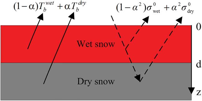
The physical temperatures of SSM/I and the backscattering coefficients of QuikSCAT based on the snow melt physical model are (Ashcraft & Long Reference Ashcraft and Long2006):
 $$T_{b} \left( 0 \right){\,\equals\,}\alpha _{1} T_{b}^{{\rm dry}} {\plus}\left( {1{\,\minus\,}\alpha _{1} } \right)T_{b}^{{\rm wet}} \quad ({\rm in}\quad {\rm K}),$$
 $$\sigma ^{0} {\,\equals\,}\left( {1{\minus}\alpha _{2}^{2} } \right)\sigma _{{\rm wet}}^{0} {\plus}\alpha _{2}^{2} \sigma _{{\rm dry}}^{0} ,$$
where, T
b
(0) is physical temperature, α1 is the attenuation coefficient of SSM/I,
 $T_{b}^{{\rm dry}} $
is the dry snow physical temperature,
 $T_{b}^{{\rm wet}} $
is the wet snow physical temperature, σ0 is the backscattering coefficient (no units), α
2 is the attenuation coefficient of QuikSCAT,
 $\sigma _{{{\rm wet}}}^{{\rm 0}} $
is the wet snow backscattering coefficient (no units),
 $\sigma _{{{\rm dry}}}^{{\rm 0}} $
is the dry snow backscattering coefficient (no units). The attenuation coefficients (
 $\alpha _{1} {\,\equals\,}e^{{{\minus}k_{{\alpha _{1} }} d_{1} \sec \theta _{1} }} $
and
 $\alpha _{2} {\,\equals\,}e^{{{\minus}k_{{\alpha _{2} }} d_{2} \sec \theta _{2} }} $
; in which, k
α
is the absorption loss coefficient, d is the wet snow depth and θ is the transmission angle) are mainly determined by the thickness of the wet snow layer. In this model, the measured emissions are near the Brewster angle, so the reflections at the interface of air/wet snow and wet snow/dry snow can be ignored. Therefore, the wet snow depths are:
 $$d_{1} {\,\equals\,}{{\ln \alpha _{1} } \over {{\minus}k_{{\alpha 1}} \sec \theta _{1} }},$$
 $$d_{2} {\,\equals\,}{{\ln \alpha _{2} } \over {{\minus}k_{{\alpha 2}} \sec \theta _{2} }},$$
which can been obtained through
 $\alpha _{1} {\,\equals\,}e^{{{\minus}k_{{\alpha _{1} }} d_{1} \sec \theta _{1} }} $
and
 $\alpha _{2} {\,\equals\,}e^{{{\minus}k_{{\alpha _{2} }} d_{2} \sec \theta _{2} }} $
. The wet snow depth is the same in the same area with SSM/I and QuikSCAT, therefore:
 $${{\ln \,\alpha _{1} } \over {{\minus}k_{{\alpha 1}} \,\sec \theta _{1} }}{\,\equals\,}{{\ln \,\alpha _{2} } \over {{\minus}k_{{\alpha 2}} \,\sec \theta _{2} }},$$
where k α1 sec θ 1=16.2220 and k α2 sec θ 2=12.7684, and therefore:
 $${{\ln \,\alpha _{{\rm 1}} } \over {16.2220}}{\,\equals\,}{{\ln \,\alpha _{2} } \over {12.7684}}.$$
Therefore, 12.7684 ln α 1=16.2220 ln α 2. This can be expressed in the exponential form as:
 $$\alpha _{2} {\,\equals\,}\alpha _{1} ^{{{{12.7684} \over {16.2220}}}} .$$
The relationship between the attenuation coefficients of SSM/I and QuikSCAT is then established, where α 1 is the attenuation coefficient for SSM/I data and α 2 is the calculated attenuation coefficient of the corresponding pixel for QuikSCAT data.
The weighting coefficient w can be defined as follows:
 $$w{\,\equals\,}{{\alpha _{2} } \over {\overline{{\alpha _{2} }} }}{\,\equals\,}\alpha _{2} \,/\,({{\alpha _{{_{1} }}^{'} {\plus}\alpha _{{_{2} }}^{'} {\plus} \cdots {\plus}\alpha _{{_{n} }}^{'} } \over n})\matrix{ {} & {(n{\,\equals\,}25)} \cr } ,$$
where
 $$\alpha _{{_{1} }}^{'} ,\alpha _{{_{2} }}^{'} , \cdots ,\alpha _{{_{n} }}^{'} $$
are the attenuation coefficients of QuikSCAT corresponding to the position of SSM/I pixels. Eq. (2) can be sorted to:
 $$\sigma ^{0} {\,\equals\,}\sigma _{{{\rm wet}}}^{{\rm 0}} {\minus}\alpha ^{2} \sigma _{{{\rm wet}}}^{{\rm 0}} {\plus}\alpha ^{2} \sigma _{{{\rm dry}}}^{{\rm 0}} .$$
Then:
 $$\sigma ^{0} {\minus}\sigma _{{{\rm wet}}}^{{\rm 0}} {\,\equals\,}\alpha ^{2} (\sigma _{{{\rm dry}}}^{{\rm 0}} {\minus}\sigma _{{{\rm wet}}}^{{\rm 0}} ).$$
In decibels, Eq. (10) (no units) can be expressed as follows:
 $$10\lg (\sigma ^{0} {\minus}\sigma _{{{\rm wet}}}^{{\rm 0}} ){\,\equals\,}20\lg \alpha {\plus}10\lg (\sigma _{{{\rm dry}}}^{{\rm 0}} {\minus}\sigma _{{{\rm wet}}}^{{\rm 0}} ).$$
Recalling that
 $$\sigma _{{{\rm wet}}}^{{\rm 0}} $$
is relatively small (Ashcraft & Long Reference Ashcraft and Long2006), the contribution from
 $$\sigma _{{{\rm wet}}}^{{\rm 0}} $$
is assumed negligible. Thus:
 $$\sigma _{{^{1} }}^{0} {\,\equals\,}20\,\lg \,\alpha {\plus}\sigma _{{{\rm dry1}}}^{{\rm 0}} \matrix{ {} \cr } \left( {{\rm in}\matrix{ {} \cr } {\rm dB}} \right).$$
Moreover, the attenuation coefficients of QuikSCAT can be obtained as:
 $$\alpha {\,\equals\,}10^{{(\sigma _{{^{1} }}^{0} {\minus}\sigma _{{\rm dry1}}^{0} )\,/\,20}} .$$
The modified backscattering coefficients of SSM/I can be obtained by the weighting (revision) coefficient w substituted into Eq. (12) as follows:
 $$\sigma _{{^{1} }}^{0} {\,\equals\,}20\,\lg (w\alpha ){\plus}\sigma _{{{\rm dry1}}}^{{\rm 0}} .$$
The attenuation coefficients and the weighting (revision) coefficients of QuikSCAT are substituted into Eq. (13), which can be used to generate the modified backscatter results.
The important steps of the snow melt detection method based on the proposed synergistic algorithm can be summarized as follows:
-
i) Calculate the brightness temperature
 $$T_{b}^{{\rm dry}} $$
and the backscattering coefficient
$$\sigma _{{\rm dry}}^{0} $$
of each pixel point;
$$T_{b}^{{\rm dry}} $$
and
$$\sigma _{{\rm dry}}^{0} $$
are estimated as the average T
b
and σ
0 from 1 June to 31 August during the winter at each location (here, in 2000 and 2001).
-
ii) Calculate the attenuation coefficient α of SSM/I by T wet≈273k and the obtained
$$T_{b}^{{\rm dry}} $$
value based on step i). -
iii) Calculate the attenuation coefficient α of QuikSCAT by the obtained
$$\sigma _{{\rm dry}}^{0} $$
value based on step i). -
iv) Resample the images of SSM/I and QuikSCAT (by using the nearest neighbour method); QuikSCAT data are resampled from the original 4.45 km to 5 km resolution, and SSM/I data are resampled from the original 25 km to 5 km resolution.
-
v)Clip the resampled images of SSM/I and QuikSCAT data; the clipping range is 1150×950.
-
vi) Calculate the attenuation coefficient of QuikSCAT with the same position used for the SSM/I; it can be calculated by Eq. (7).
-
vii) Find the correction coefficient w of QuikSCAT; it can be obtained by:
(15)
$$w{\,\equals\,}{{\alpha _{1} } \over {\overline{{\alpha _{2} }} }}{\,\equals\,}\alpha _{1} \,/\,({{\alpha _{{_{1} }}^{'} {\plus}\alpha _{{_{2} }}^{'} {\plus} \cdots {\plus}\alpha _{{_{n} }}^{'} } \over n}).$$
-
viii) The backscattering coefficient of each pixel point can be obtained by Eq. (14) for QuikSCAT data.
-
ix) Produce Antarctic snow melt maps based on the snow melt physical model proposed by Ashcraft & Long (Reference Ashcraft and Long2006) with a threshold of 2.8 dB. Melt detection is based on thresholding some melt signal (q(t)) which varies with time. Let m(t) represent the melt detection with m=1 indicating melt and m=0 indicating non-melt, i.e:


 $$m\left( t \right){\,\equals\,}\left\{ \matrix{ 1\matrix{ {} \cr } {\rm if}\matrix{ {} \cr } q\left( t \right){\,\equals\,}\sigma _{{{\rm dry}}}^{{\rm 0}} {\,\minus\,}\sigma ^{0} \geq 2.8 \hfill \cr 0\matrix{ {} \cr } {\rm if}\matrix{ {} \cr } q\left( t \right){\,\equals\,}\sigma _{{{\rm dry}}}^{{\rm 0}} {\,\minus\,}\sigma ^{0} \,\lt\,2.8 \hfill \cr} \right..$$
Results
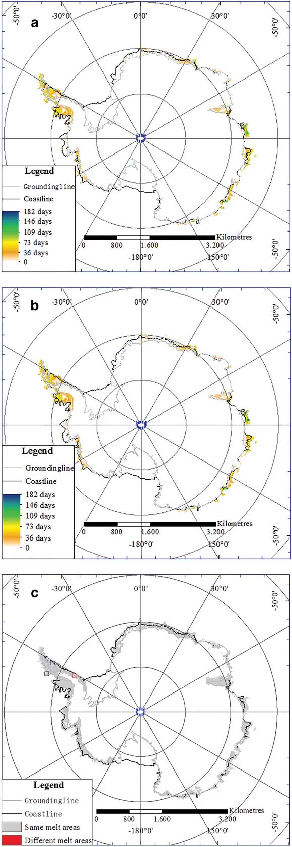
First, the correction coefficients for QuikSCAT data for every pixel point were calculated. Then, the modified backscattering coefficients were obtained. Finally, the Antarctic snow melt maps based on the synergistic data and QuikSCAT data from 1 October 2000 to 31 March 2001 (shown in Fig. 2) were obtained with a threshold of 2.8 dB and use of the snow melt physical model for microwave radiometer and scatterometer data.
Snow melt duration with a. QuikSCAT data and b. the synergetic method. c. Differences between the two methods. Red box = Butler Island, blue box = Larsen Ice Shelf, black box = Bonaparte Point.
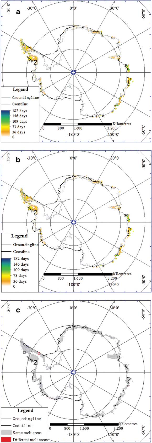
Figure 2a & b shows that snow melt duration and distribution were the same for most pixels, and that there are 210 different pixel points for snow melt duration (Fig. 2c and Table I).
Different pixel points for snow melt duration.

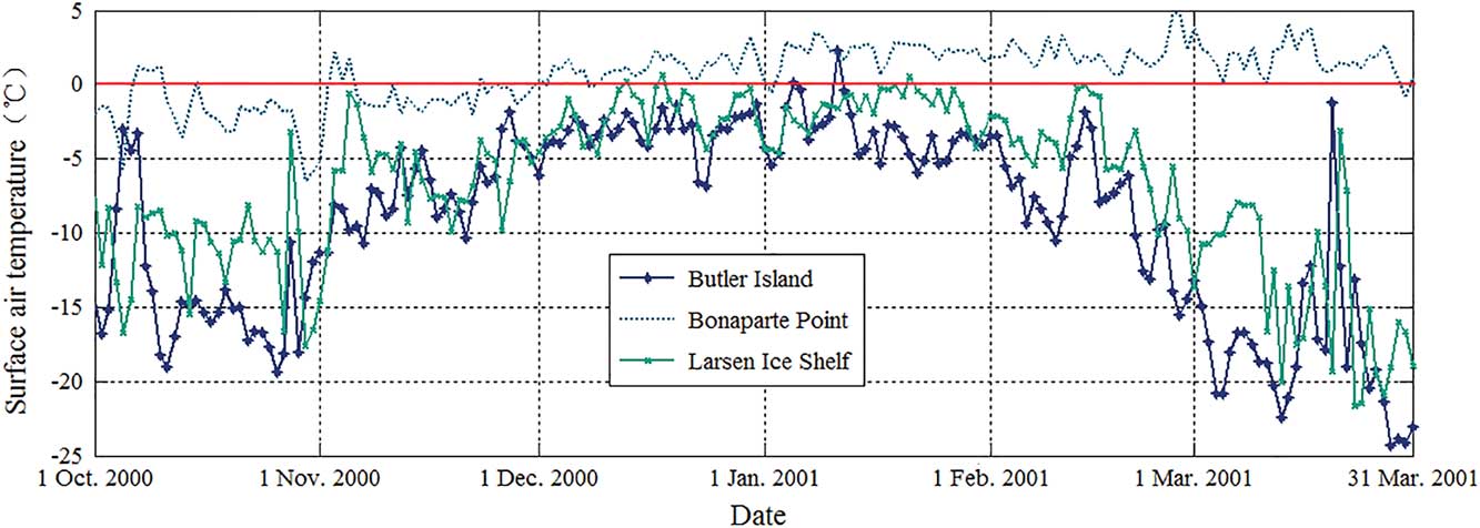
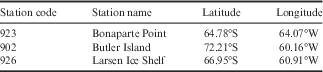
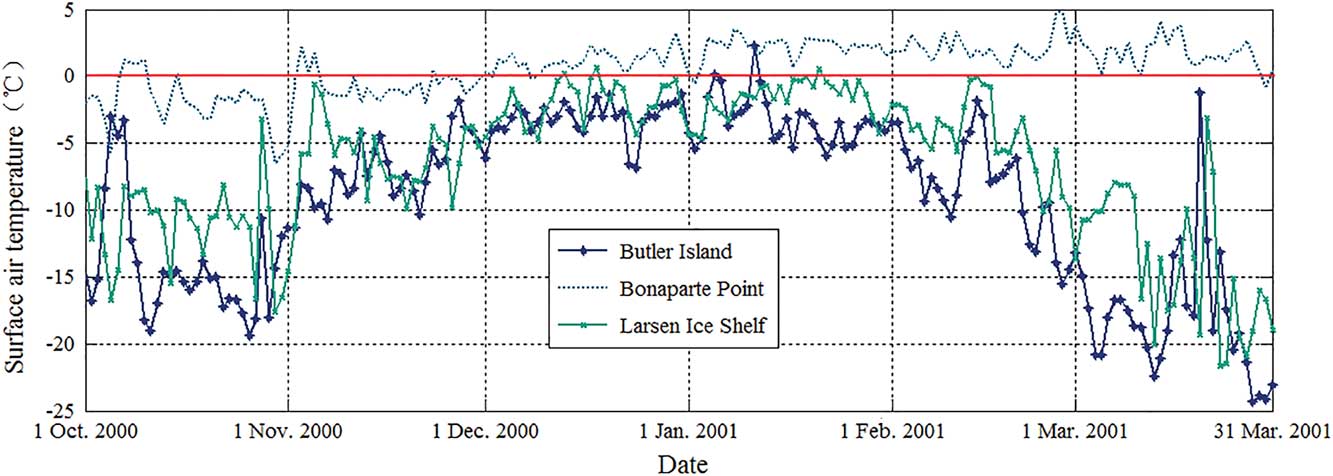
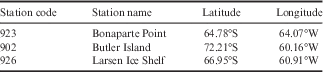
The different pixels were located in the region bordering Antarctica, and these pixels were affected by the complex terrain. To verify that the snow melt estimates obtained by the proposed synergetic method had a higher accuracy than those obtained with the original method, three regions with 10×10 zoom-in pixel points (as shown in Fig. 2c) were selected where the temperature data were collected from three AWSs (see Table II for details) at wet snow points (Fig. 3).
Temperature changes at Bonaparte Point, Butler Island and the Larsen Ice Shelf from 1 October 2000 to 31 March 2001.
Geographical information for the automatic weather stations.
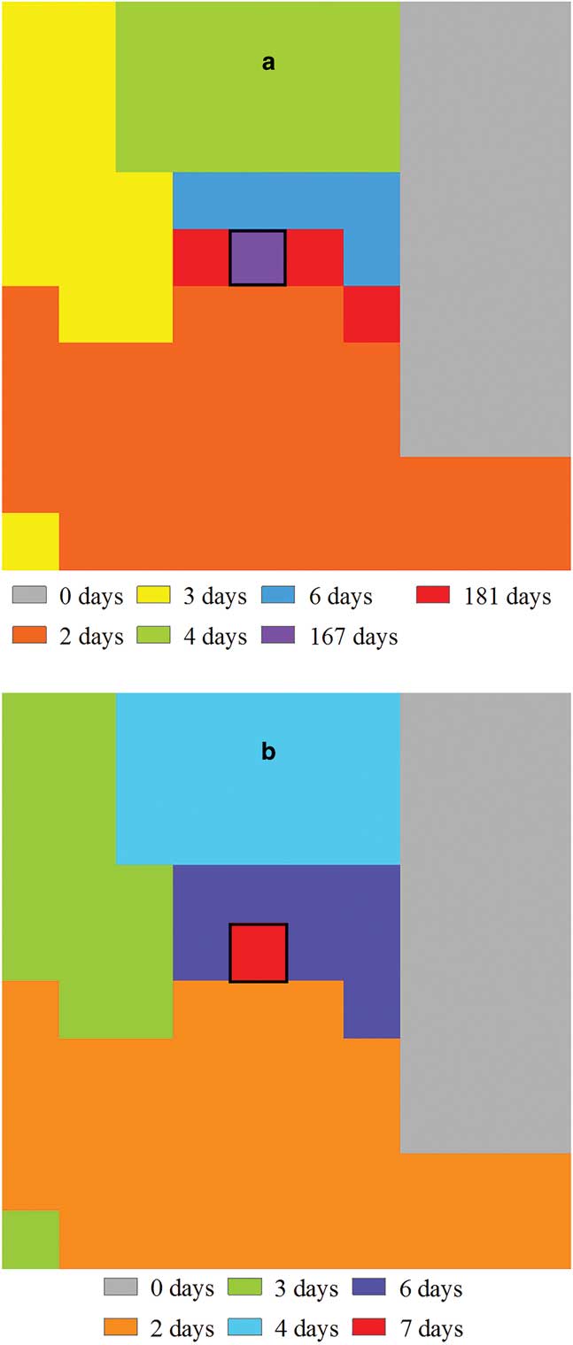
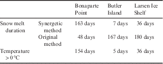
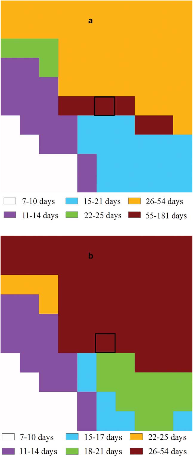
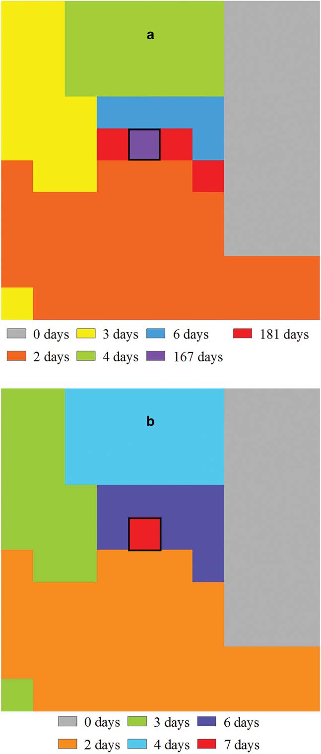
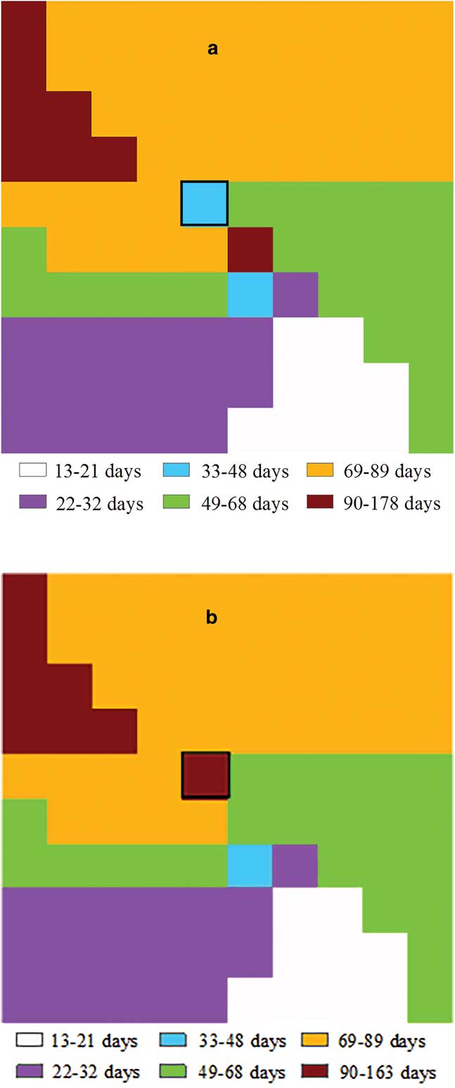
The snow melt duration for the pixel point where Bonaparte Point is located (black box pixel in Fig. 4) was 163 days according to the synergetic method compared with 48 days with the original method (Table III). The estimate of the synergetic method is more consistent with the number of days (154 days) that the temperature was >0 °C.
Snow melt duration at Bonaparte Point (black box in Fig. 2c) with a. QuikSCAT data and b. the synergetic method.
Comparison of temperature and snow melt duration (synergetic and original methods) data from the automatic weather stations.
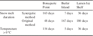
For the pixel point where Butler Island is located (black box pixel in Fig. 5) the snow melt duration was seven days with the synergetic method, which is similar to the number of days (five days) that the temperature was >0 °C (Table III). The estimated snow melt duration with the original method was 167 days. Again, the estimate of the synergetic method is more consistent with the number of days >0 °C.
Snow melt duration at Butler Island (red box in Fig. 2c) with a. QuikSCAT data and b. the synergetic method.

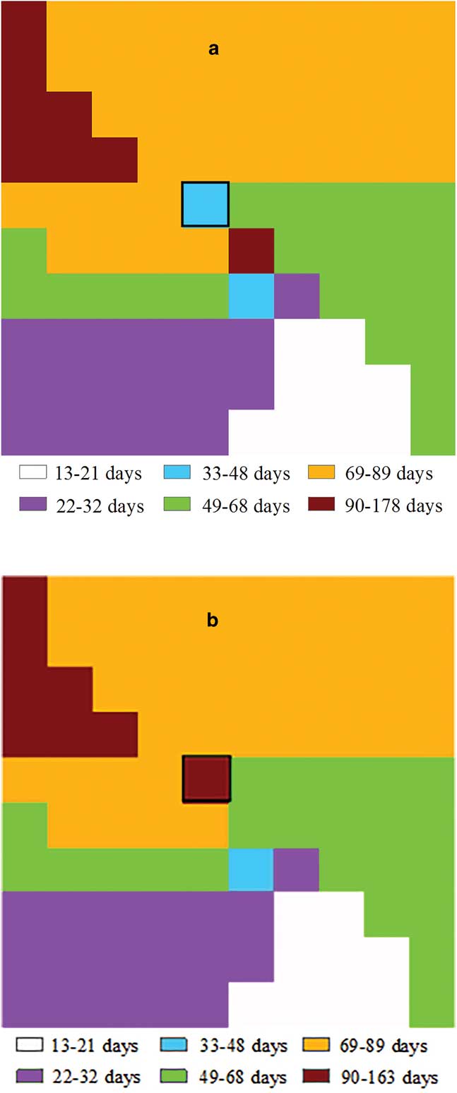
For the pixel point where the Larsen Ice Shelf is located (black box pixel in Fig. 6) the snow melt duration was estimated at 36 days with the synergetic method, exactly the same as the number of days that the temperature was >0 °C, compared with 180 days with the original method (Table III). Thus, the synergistic approach should be effective for obtaining accurate Antarctic snow melt estimates.
Snow melt duration at the Larsen Ice Shelf (blue box in Fig. 2c) with a. QuikSCAT data and b. the synergetic method.
Discussion
The brightness temperatures of SSM/I and the backscattering coefficients of QuikSCAT are very sensitive to the appearance of liquid water in snow, and snow melt information can be obtained through the snow melt physical model using SSM/I and QuikSCAT data. Both SSM/I and QuikSCAT data have their own characteristics and advantages in snow melt detection, i.e. SSM/I data has higher reliability (there are smaller effects of surface roughness, surface morphological changes, etc) and QuikSCAT data has higher spatial resolution. Here, the advantages of SSM/I and QuikSCAT data have been combined to complement each other. Comparison of temperature data from three AWSs with snow melt estimates made using the synergetic method and the original method shows that the proposed method can improve the accuracy of snow melt detection.
Since the SSM/I and QuikSCAT data have low spatial resolution (SSM/I: 25×25 km, QuikSCAT: 4.45×4.45 km, synergetic method: 5×5 km) it is difficult to validate estimates of snow melt (i.e. it is difficult to accurately quantify a temperature AWS data point to verify the snow melt), and most research is based on either comparative verification with different algorithms or qualitative analysis. In addition, snow melt is affected by temperature, terrain, slope, aspect and altitude; therefore, the temperature data from three AWSs can only be used to qualitatively explain that the proposed method may improve the detection accuracy to some extent.
In future studies, the synergetic method will be applied to other regions. We believe that the proposed method will provide support for and supplement global snow melt detection.
Conclusion
The proposed synergistic algorithm based on SSM/I and QuikSCAT data improved the accuracy of snow melt estimates in Antarctica compared to traditional methods. This new synergetic algorithm could also be applied to other areas, which would provide further evidence to support its use and additional data to document changes in the Antarctic due to global climate change.
Acknowledgements
This research was supported by the National Natural Science Foundation of China (No. 41606209); the National Key Research and Development Program of China (No. 2016YFB0501501), Fujian Provincial Key Laboratory of Photonics Technology, Key Laboratory of Optoelectronic Science and Technology for Medicine of Ministry of Education, Fujian Normal University, China (No. JYG1707); Polar Science Strategic Research Foundation of China (No. 20150312); the Fundamental Research Funds for the Henan Provincial Colleges and Universities (No. 2015QNJH16); the science and technology project of Zhengzhou Science and Technology Bureau (No. 20150251); and high-level talent scientific research fund item of Henan University of Technology (No. 150525). We thank the Editor and the anonymous reviewers for their time and effort, which significantly improved this manuscript.
Author contributions
XW and XL conducted the mapping from SSM/I and QuikSCAT data, carried out the analyses and interpretation of the data, and led the writing of the manuscript. All authors discussed the results and implications, and commented on the manuscript at all stages.