1. INTRODUCTION
A comprehensive map of global shipping density is fundamental for Maritime Situational Awareness (MSA), which consists of vessel and traffic density. The definition of vessel density in a region was taken as the expected number of vessels per unit area at any time, and traffic density as the average number of vessels crossing this region per unit area per unit time. Considering that maritime transportation represented approximately 80% of global trade by volume in 2014 (United Nations Conference on Trade and Development (UNCTAD), 2015), MSA is essential for the detection of incidents such as piracy, accidents, smuggling, and terrorism to protect the safety of life at sea. In addition to safety, the situation and trends of shipping density will also have important economic value.
According to the International Convention for the Safety of Life at Sea (IMO, 1974), ships of 300 gross tonnes and upwards on international voyages, 500 tonnes and upwards for cargos not in international waters and passenger vessels are required to fit an AIS transceiver (ITU-R, 2010), which broadcasts kinematic (dynamic) and identity (static) information automatically. AIS data is now an important source of information for MSA.
The Maritime Mobile Service Identity number (MMSI) in AIS messages broadcast by each ship is supposed to be unique, and it was used by Pallotta et al. (Reference Pallotta, Vespe and Bryan2013a) to identify and track each vessel. It is not unusual that a MMSI is shared by different vessels (Mazzarella et al., Reference Mazzarella, Alessandrini, Greidanus, Alvarez, Argentieri, Nappo and Ziemba2013), as this field is input manually and not considered reliable. In this instance, vessels will appear to jump quickly on the map, distorting their real tracks and shipping density maps. In the study of AIS data received from 23 November 2005 to 2 May 2006 mainly in European waterways (Harati-Mokhtari et al., Reference Harati-Mokhtari, Wall, Brooks and Wang2007), there were up to 25 vessels transmitting the incorrect MMSI number of 1193046. The authors supposed that this number might be the default MMSI for a specific model of AIS transponder. Greidanus et al. (Reference Greidanus, Alvarez, Eriksen, Argentieri, Çokacar, Pesaresi, Falchetti, Nappo, Mazzarella and Alessandrini2013) listed 5155 distinct MMSIs which were reported from 5235 distinct ships over the Gulf of Aden and the Western Indian Ocean during one month. This situation is much worse when global data is observed, because the probability of duplication increases when the number of ships rises to hundreds of thousands. To remove noise, Pallotta et al. (Reference Pallotta, Vespe and Bryan2013a) eliminated duplicate data resulting from different ships using the same MMSI using velocity gating. Instead of eliminating data, Mazzarella et al. (Reference Mazzarella, Alessandrini, Greidanus, Alvarez, Argentieri, Nappo and Ziemba2013, Reference Mazzarella, Vespe, Damalas and Osio2014) adopted a nearest neighbour method to assign AIS messages to ships. However, their methods were only applied in small areas, and no information was given about the performance and results.
The wide use of AIS makes automatic analysis of global shipping possible. However, related works were focused at regional and national scales for periods ranging from several days to a year (Arguedas et al., Reference Arguedas, Pallotta and Vespe2014; Holsten, Reference Holsten2009; MMO, 2014a; Pallotta et al., Reference Pallotta, Vespe and Bryan2013a; Shelmerdine, Reference Shelmerdine2015). MMO (2014b) and Shelmerdine (Reference Shelmerdine2015) both reported a processing time of one day for one month's AIS data. Although these studies carried out a significant amount of quality control within their processing, it would be necessary to reduce this processing time for AIS to be examined at a global level.
To monitor the coverage of global AIS receiving networks (including base stations and satellites), it is important to have AIS receiving frequency maps to find weak coverage areas, which is relatively unexplored in previous works. To eliminate the influence of vessel density, the definition of AIS receiving frequency in a region was taken as the expected number of received distinct messages broadcast by any single vessel per unit time when the vessel is in this region. A high value of AIS receiving frequency in a region indicates low packet loss rate.
There are two types of methods of analysing traffic: grid-based and vector-based. Grid-based methods were the most widely used in the literature (MMO, 2014a; Natale et al., Reference Natale, Gibin, Alessandrini, Vespe and Paulrud2015; Pan et al., Reference Pan, Jiang, Hu and Shao2012; Shelmerdine, Reference Shelmerdine2015), which subdivided the area of interest into grids and characterised them using various properties. The processing rate was reported in only a few works. It took Shelmerdine (Reference Shelmerdine2015) one day to process a month of data (from 16,999 to 122,355 records). To reduce the amount of data and processing time, the Marine Management Organisation (MMO) performed transit identification and thinning before processing (MMO, 2014b), which took 30 to 100 hours per week of data around the UK (between latitudes 47°N and 65°N and between longitudes 10°W and 10°E) depending on PC specifications and hardware. Grid-based methods have been considered effective only for small area surveillance and the computational burden was regarded as its limitation when increasing the scale (Pallotta et al., Reference Pallotta, Vespe and Bryan2013a, Reference Pallotta, Vespe and Bryan2013b, Reference Pallotta, Vespe and Bryan2013c; Vespe et al., Reference Vespe, Visentini, Bryan and Braca2012). Therefore a “vectorial” representation of traffic was proposed (Arguedas et al., Reference Arguedas, Pallotta and Vespe2014) to allow implementation at a global scale, including waypoint objects and route objects. However, these methods had only been implemented in bounding areas (e.g. a 200 × 160 km area in the North Adriatic Sea (Pallotta et al., Reference Pallotta, Vespe and Bryan2013c) and the Dover Strait (Arguedas et al., Reference Arguedas, Pallotta and Vespe2014)), and no information was given about performance.
There are two important problems to be studied when mapping global shipping density from AIS data: duplication of MMSIs and implementation of algorithms on a global scale. The aim of this work was to describe a pre-processing method to discriminate different ships using the same MMSI on a global scale, which takes both spatial and temporal factors into consideration. The use of a grid-based method for computing shipping density, which is fast enough when implemented at a global scale, will be demonstrated. The performance and results of pre-processing, as well as shipping density computation will also be addressed.
2. MATERIALS AND METHODS
The China Transport Telecommunications and Information Centre (CTTIC) provided us with 21,162,882,025 pieces of dynamic data and 635,055 pieces of static data. Each piece of static data was the last record received from a MMSI. Due to some flaws in CTTIC's system, static data of some ships was not in the dataset. This problem will be solved in the near future. The data sources of CTTIC include AISHub, ORBCOMM, China's Maritime authorities and universities, etc. AIS messages can also be broadcast by coast stations and handheld VHF transceivers. These were excluded by limiting the first digit of a MMSI within the range from 2 to 7, which was used by individual ships. To further improve the quality of data, only ships with valid names (non-empty) and types (between 20 and 99) were taken into consideration. These AIS records were from August 2012 to May 2015, 34 months in total. All these 21 billion records were pre-processed in Section 2.1 and 20 billion records from the former 33 months were used to study shipping density in Section 2.2, as the data for the last month (about one billion pieces) was incomplete. All of these records were in a single table of MySQL Community Server 5·6·24. This table was partitioned by MMSI, with MMSI and timestamp as the primary key. In this way, data in the table were ordered by MMSI and timestamp, speeding up the retrieval. After pre-processing, data were inserted into a second table, which was partitioned by timestamp (one month per partition) with ship ID and timestamp as the primary key, facilitating retrieval as well as incremental processing. The MySQL server ran on a CentOS server with 2 × Xeon E5 2620v2 CPU, 16 × 8 GB DDR3 1600 MHz RAM and 8 × 3TB SAS disk. All of the processing programs ran on another server of the same model, using C++.
2.1. Pre-Processing and Data Association
The main task in the pre-processing step of our work was to associate each AIS dynamic record to an existing or new ship ID. The likelihood of the association between an AIS dynamic record and each candidate ship ID was calculated according to their spatial and temporal proximity, see Algorithm 1. In the algorithm, D is a record of AIS dynamic data, V i is one of the vessels whose MMSI is the same as that of D, l is the likelihood that D was broadcast by V i , Pos1 and Pos 2 are two pieces of AIS dynamic data broadcast by V i and their timestamps are prior to and after that of D respectively, Dis 1 is the distance between D and Pos 1 , Dis2 is the distance between D and Pos 2 , t1 is the time between D and Pos 1 , t2 is the time between D and Pos 2 . According to MarineTraffic, among 72,371 ships within the range of its worldwide AIS receiving networks when accessing the website, only 94 ships had a speed equal to or above 30 knots (MarineTraffic, 2016a). So the speed of a ship is unlikely to be more than 30 knots, which was the value of Speed thr in the algorithm. Among these craft, only one had a speed equal to or above 45 knots (MarineTraffic, 2016b), which was a Search And Rescue (SAR) aircraft. The maximum and average speed of this aircraft was 133 and 87·6 knots respectively (MarineTraffic, 2016c). So it is almost impossible for the speed of a ship to be more than 120 knots, which was the value of Speed max in the algorithm. When two positions are within a small range Dis proxi (set empirically as 100 kilometres) and from the same MMSI, then it was very likely that they were reported by the same ship regardless of computed speed. Due to errors such as imprecise timestamp, the computed speed of a ship may be extremely high.
Computing the likelihood that a record of AIS dynamic data was from a vessel Vi

In most cases, each record would be associated to the vessel with the maximum likelihood. When the track of one ship was split into several parallel ones erroneously, subsequent AIS records would be associated to one of these tracks almost randomly. To converge these tracks in this situation, when at least two likelihood values were not less than 0·8, this AIS record was assigned to the ‘freshest’ ship whose last message was newest. The threshold value 0·8 was set empirically, and the likelihood was above it when the average speed between the record and the candidate track was below 10 knots or when the distance between them was less than 100 kilometres (see Algorithm 1). When the maximum likelihood was not above zero, this record was considered as from a new ship and this ship was assigned a new ship ID. After data association, new ships with only a few records were regarded as noise and moved to a separate table named “L1_Noise_Ship_History_Positions”.
The threshold values used in our work for classifying duplicated MMSIs were looser than those used by Greidanus et al. (Reference Greidanus, Alvarez, Eriksen, Argentieri, Çokacar, Pesaresi, Falchetti, Nappo, Mazzarella and Alessandrini2013), trying to lower the false positive rate. For example, in Greidanus et al. (Reference Greidanus, Alvarez, Eriksen, Argentieri, Çokacar, Pesaresi, Falchetti, Nappo, Mazzarella and Alessandrini2013), a speed of >45 knots and two positions farther than 2·25 NM will be regarded as two ships. While in our paper, these two numbers were 120 knots (Speed max ) and 100 kilometers (Dis proxi ) respectively.
2.2. Shipping Density Analysis
Global vessel density and traffic density maps were calculated based on 15 ship types output by the AIS system (ITU-R, 2010). All these maps were output in three different spatial resolutions: 1° latitude by 1° longitude, 10 minutes latitude by 10 minutes longitude, and 1 minute latitude by 1 minute longitude. AIS receiving frequency maps were also computed to reflect the coverage of AIS receiving networks.
The temporal resolution of these maps were one month, which was refined enough to reflect shipping density variation in most cases and can be further aggregated into seasonally and yearly density maps. When analysing shipping density, the motion between two successive records in a track was assumed uniform to compute the length and time the ship sailed in each grid. When analysing shipping density, if the likelihood of a record was below 0·7, or time interval between two successive positions was more than one day, the track ends there.
2.2.1. Vessel Density Analysis
The vessel density in a region at time t is the number of vessels per unit area in this region at this time. The vessel density in a region from time t to t + T was defined as the expected value of vessel density in this region during the period. According to this definition, the vessel density in grid_i in month_m can be calculated as:
 $$ShipDensity_i^m = \displaystyle{{\mathop \sum \nolimits_{s = 1}^{s = ship\_count} Time_i^s} \over {Time_{month\_m} \ {^\ast}Area_{grid\_i}}} = \displaystyle{{CrossingTimeSum_i} \over {Time_{month\_m} \ {^\ast}Area_{grid\_i}}} $$
where ship_count is the number of ships recorded in this area in month_m, Time i s is the total time that the s-th ship stayed in this grid, Time month_m is the total time of this month, Area grid_i is the area of this grid, CrossingTimeSum i is the sum of the time stayed by all the ships in this grid in this month.
2.2.2. Traffic Density Analysis
Traffic density represents how many vessels crossed a unit area per unit time. The traffic density in a region from time t to t + T was defined as the average number of vessels which cross this region per unit area per unit time. According to this definition, the traffic density in grid_i in month_m can be calculated as:
 $$TrafficDensity_i^m = \displaystyle{{\mathop \sum \nolimits_{s = 1}^{s = ship\_count} CrossingCount_i^s} \over {Time_{month\_m} \ {^\ast}Area_{grid\_i}}} = \displaystyle{{CrossingCountSum_i} \over {Time_{month\_m} \ {^\ast}Area_{grid\_i}}} $$
where ship_count is the total number of ships which crossed grid_i in month_m, CrossingCount i s is the count that the s-th ship crossed this grid this month, Time month_m is the total time of this month, Area grid_i is the area of this grid, CrossingCountSum i is the sum of the count that each ship crossed this grid this month.
When a ship is on the border of two or more grids, it may jump between these grids continuously, enlarging the traffic density of these grids. To solve this problem, a queue was used to record the recent grids the vessel under analysis had crossed.
2.2.3. AIS Receiving Frequency
The definition of AIS receiving frequency in a region was taken as the expected number of received distinct messages broadcast by any single vessel per unit time when the vessel was in this region. AIS receiving frequency maps reflect the coverage of AIS networks. The AIS receiving frequency in the i-th grid in month_m was calculated as follows:
 $$F{\rm req}_i^m = \displaystyle{{\mathop \sum \nolimits_{s = 1}^{ship\_count} AIS\_Count_i^s} \over {\mathop \sum \nolimits_{s = 1}^{ship\_count} Time_s}} = \displaystyle{{AISCountSum_i} \over {CrossingTimeSum_i}} $$
where AIS_Count i s is the number of messages received from s-th ship when it is in grid_i, Time s is the total time that the s-th ship spent in this grid, AISCountSum i is the total number of messages received from ships in this grid this month, CrossingTimeSum i is the sum of time that each ship spent in this grid.
To derive these three types of maps, three properties for each grid need to be calculated: CrossingTimeSum, CrossingCountSum and AISCountSum. In the program of density computing, tracks of each ship were traversed and properties of grids crossed were updated. As data was ordered by ship ID and timestamp in the table, the program just traversed the table sequentially once.
3. RESULTS
The program of association ran with 20 threads, and completed the task after 16 hours and 10 minutes. The results showed that the 21,162,882,025 records of AIS dynamic data came from 1,998,200 distinct MMSIs and, of these, 1,607,664 MMSIs had broadcast only 18,167,656 messages in total which were regarded as noise. The other 390,536 MMSIs were shared by 491,346 different vessels, and 21,144,714,369 messages had been received from them. Among the 390,536 MMSIs, there were 308,279 which had not been used by more than one vessel. The total number of vessels which had broadcast during the first five months of 2015 was 368,186, sharing 317,108 MMSIs. MMSIs like 123456789, 111111111, 999999999, 222222222, 100000000, 888888888, 413000000, and 808664168, had been shared by more than ten vessels.
More than 99·9% of the final likelihood computed by Algorithm 1 was above 0·7. Lower likelihood denotes smaller confidence in the association, which may result from an unlikely high speed, large time intervals, or a suspiciously long distance between two AIS records. It took 56 hours to produce all the global monthly ship density, traffic density and AIS receiving frequency maps, from August 2012 to April 2015; 33 months of data. This equated to an average of 1·7 hours processing per month's global data.
Maps at the resolution of 1° by 1° were used mainly for previewing the data, and are not shown here. Data at a resolution of 10 minutes by 10 minutes was used when observing shipping density globally. When more detail was required about a specific area, data at a resolution of 1 minute by 1 minute was examined. The colours used in the map outputs are shown in Figure 1.
The colours from left to right represent a rising value of vessel density/traffic density/AIS. receiving frequency from low to high.

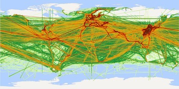
To verify the impact of pre-processing, the global shipping density from the raw AIS data in April 2015 (latest month of the data used for shipping analysis) was computed for comparison. The traffic density map is depicted in Figure 2, which was overwhelmed by noisy lines crossing continents resulting from ships in different areas sharing MMSI numbers. When a ship jumped between two areas frequently, the line connecting them would appear to have high traffic density. There were many lines connecting points spanning almost half of the earth, indicating how severe the problem was when analysing global shipping. There were also some vertical and horizontal lines in the map, probably due to a reset or error of a device. During the pre-processing of our work, those AIS records due to reset or error would be regarded as from another ship with the same MMSI at first. Then they would be recognised as noise and no ship ID would be created for them, because the “ship” had broadcast only a few messages.
Global traffic density maps in April, 2015, based on the data before pre-processing. The spatial resolution is 10 minute longitude by 10 minute latitude.

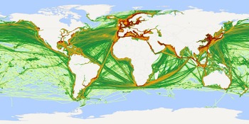
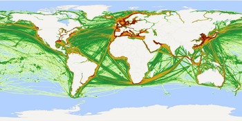
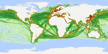
As a comparison, in the traffic density map of the same period (April 2015), based on pre-processed data, noisy lines on continents as well as those vertical and horizontal lines were hardly seen (Figure 3). From traffic density maps of different months, some obvious variations over time can be observed. For example, during April, in Russia and Canada, traffic on the rivers was hardly seen, probably due to the cold temperatures freezing the water, but traffic routes were noted between South America and Antarctica (Figure 3). By September, traffic routes on the rivers of Russia and Canada appeared, while Antarctica witnessed a gradual decline of visits (Figure 4).
Global traffic density in April, 2015, at the spatial resolution of 10 minutes longitude by 10 minutes latitude.

Global traffic density in September, 2014, at the spatial resolution of 10 minutes longitude by 10 minutes latitude.

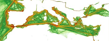
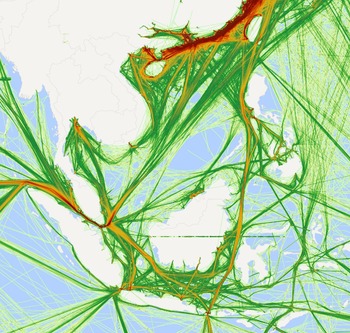
With density maps at a finer resolution, more details were observed (Figures 5 and 6) which represented the traffic density around the Mediterranean Sea and Southeast Asia, respectively. The traffic separation scheme along the west coast of Portugal was clearly observed as high density (Figure 5). From the dense straight lines connecting numerous ports along the Mediterranean Sea, it can be concluded that there were tight connections among these ports. Constrained by masses of islands and reefs in Southeast Asia, curved traffic routes as well as “holes” were commonly observed (Figure 6). The Strait of Malacca seemed a bottleneck considering the extremely dense traffic there, influencing the shipping of products made in Southeast Asia to the West.
Traffic density around Mediterranean Sea in April, 2015, at the spatial resolution of 1 minute longitude by 1 minute latitude.

Traffic density in Southeast Asia in April, 2015, at the spatial resolution of 1 minute longitude by 1 minute latitude.

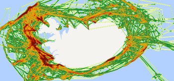
The patterns of fishing vessels’ tracks were chaotic (Figures 7 and 8). In contrast, traffic density maps of cargo ships and tankers were much more regular (Figures 9 and 10, respectively), because these ships tended to seek the shortest path to their destination.
Global traffic density of fishing ships in April, 2015, at the spatial resolution of 10 minutes longitude by 10 minutes latitude.

Traffic density of fishing ships around Iceland in January, 2014, at the spatial resolution of 10 minutes longitude by 10 minutes latitude.

Global traffic density of cargo ships in April, 2015, at the spatial resolution of 10 minutes longitude by 10 minutes latitude.

Global traffic density of tankers in April, 2015, at the spatial resolution of 10 minutes longitude by 10 minutes latitude.

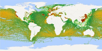
A global vessel density map reflects the expected number of vessels per unit area when observing the world. From Figure 11, the distribution of vessels in April, 2015 can be observed. Apart from busy routes, a high density of ships was also found in some isolated points, see the dots in the figure.
Global vessel density in April, 2015, at the spatial resolution of 10 minutes longitude by 10 minutes latitude.

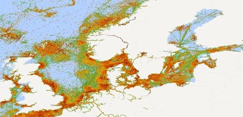
AIS receiving frequency maps represented the expected number of AIS messages received by base stations and satellites from any single ship per unit time when it was in a specific area (Figures 12 and 13). Low receiving frequency indicates weak coverage of AIS receiving networks, and can serve as a guide for maintenance and construction of base stations.
Global AIS receiving frequency in April 2015, at the spatial resolution of 10 minutes longitude by 10 minutes latitude.

AIS receiving frequency around Nordic Europe in August, 2014, at the spatial resolution of 10 minutes longitude by 10 minutes latitude.

4. DISCUSSION
In this paper, three types of density maps were defined and computed: vessel density, traffic density and AIS receiving frequency maps. The former two represented the flow and distribution of ships respectively, and the latter reflected the coverage of AIS receiving networks.
Traffic was commonly studied by visualising AIS points on maps. For example, in the work of Vespe et al. (Reference Vespe, Greidanus and Alvarez2015), traffic crossing the Indian Ocean was represented by isolated AIS points. This type of map had no information about the sequence of points and was distorted by various coverage qualities of AIS receiving networks. In comparison, traffic density maps in our paper were more informative and better approximated the real situation.
Vessel density analysis has not been greatly explored in previous works. The term “ship density” was represented as messages per grid in the work of Greidanus et al. (Reference Greidanus, Alvarez, Eriksen and Gammieri2016). As a result, the density maps demonstrated in their work were actually “AIS message density” maps. Besides, as routes between consecutive AIS records were not deduced, the computed ship density maps were full of isolated points. In our paper, vessel density maps reflected the expected number of vessels per unit area when observing the world. Places of interest can be discovered by observing high density areas. For example, in the global vessel density map in Figure 11, isolated dots along coasts with large numbers of ships can be observed. In most cases, each of them corresponds to a port.
Different types of vessels may have quite different activity patterns. For example, vessels have slower speed and irregular tracks (Mazzarella et al., Reference Mazzarella, Vespe, Damalas and Osio2014) when they are engaged in fishing (Figures 7 and 8). Shipping density analysis of different ship types was performed in this paper. It was preliminarily found that traffic density maps of fishing vessels might be good indications of probable fishing activities but this information would have to be quality controlled at the local level. For instance, these results in Figure 8 compare well with those of Mazzarella et al. (Reference Mazzarella, Vespe, Damalas and Osio2014) of the same period around Iceland.
AIS coverage maps are needed to mitigate the ambiguities between actual absence of ships and lack of receiver coverage. Besides, they can serve as an important reference for the maintenance of receiver networks. Natale et al. (Reference Natale, Gibin, Alessandrini, Vespe and Paulrud2015) used the ratio between AIS positions and trajectory interpolated points to estimate coverage capabilities. In our paper, AIS receiving frequency was defined and computed to evaluate the coverage condition. The weak coverage areas in Figure 13 were similar to those found by Natale et al. (Reference Natale, Gibin, Alessandrini, Vespe and Paulrud2015).
5. CONCLUSIONS
The wide adoption of AIS makes the computation of global shipping density possible. However, terms like “shipping density”, “ship density” and “traffic density” were used without definition in previous literature. In this paper, three terms have been defined and equations were given for computing them: vessel density, traffic density and AIS receiving frequency.
Existing works on computing shipping density were focused at regional and national scales for periods ranging from several days to a year. This paper analysed shipping density at a global scale with just over 2·5 years of data. The results of pre-processing showed that, among 1,998,200 distinct MMSIs recorded, 1,607,664 were suspicious: the average number of AIS messages broadcast by each of them was only 11·3. The remaining 390,536 MMSIs were used by 491,346 vessels. Considering the threshold values used in our work were much looser than those used by Greidanus et al. (Reference Greidanus, Alvarez, Eriksen, Argentieri, Çokacar, Pesaresi, Falchetti, Nappo, Mazzarella and Alessandrini2013), the real condition is probably much worse. After pre-processing, global vessel density, traffic density and receiving frequency maps were computed by a grid-based method. It took on average 28·5 minutes and 1·7 hours for the pre-processing and shipping density analysis of one month's data, fast enough for global shipping density analysis. Global vessel density, traffic density, and AIS receiving frequency maps as well as some regional density maps were demonstrated in this paper.
Some of the threshold parameters used in the pre-processing were set empirically, and we plan to adjust them according to results of data mining as well as expert knowledge. The false positive and false negative rates of the data association algorithm in the pre-processing step need to be examined. As there are still various types of errors in the AIS data, more work on data quality control needs to be done. Future work should include mining points of interest like anchorages and moorings. Combining shipping density maps and points of interest would make it possible to perform anomaly detection.
ACKNOWLEDGEMENTS
China Transport Telecommunications & Information Centre is thanked for providing AIS data. The reviewers are thanked for their comments that have improved the paper.
FINANCIAL SUPPORT
This work was supported by Important National Science & Technology Specific Projects (grant number 2014ZX03006–003).