Introduction
The number of detectable (i.e. communicating) extraterrestrial civilizations in the Milky Way galaxy is usually calculated by using the Drake equation (Burchell Reference Burchell2006). This equation was established in 1961 by Frank Drake and was the first step to quantifying the Search for ExtraTerrestrial Intelligence (SETI) field (Drake Reference Drake, Mamikunian and Briggs1965). This formula is broadly used in the fields of exobiology and the SETI. Practically, this equation is rather a simple algebraic expression and its simplistic nature leaves it open to frequent re-expression (Walters et al. Reference Walters, Hoover and Kotra1980; Shermer Reference Shermer2002; Burchell Reference Burchell2006; Forgan Reference Forgan2009). While keeping in mind that other equivalent forms exist, we investigate the following form:
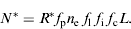
In this expression, the symbols have the following meanings: N is the number of Galactic civilizations that can communicate with Earth; R* is the average rate of star formation per year in our galaxy; f p is the fraction of stars that host planetary systems; n e is the number of planets in each system which are potentially habitable; f l is the fraction of habitable planets where life originates and becomes complex; f i is the fraction of life-bearing planets that bear intelligence; f c is the fraction of intelligence bearing planets where technology can develop; and L is the mean lifetime of a technological civilization within the detection window.
An additional problem of the Drake equation is the time-independence of its terms (Cirkovic Reference Cirkovic2004a, Reference Cirkovicb), which for example excludes the effects of the physico-chemical history of the galaxy (Forgan Reference Forgan2009). Indeed, Cirkovic (Reference Cirkovic2004a, Reference Cirkovicb) shows that the main shortcoming of the Drake equation is its lack of temporal structure, i.e., it fails to take into account various evolutionary processes that form a prerequisite for anything quantified by f parameters and n e. This Drake equation's drawback was mentioned earlier by Franck Drake but the discussion of systematic biases following such simplification was avoided (Drake & Sobel Reference Drake and Sobel1991).
In particular, not only some difficulties arise from changing one or more parameters values in equation (1) with time, but also the Drake equation does not provide any error estimation about the measured quantity. To be short, a estimation of N=5 with a standard deviation (SD) SD(N)<<1 is radically different from an estimation of N=10 with a standard error of SD(N)=10. Recently, Maccone (Reference Maccone2010) derived the first statistical Drake equation by associating each parameter with a random variable and then, given some assumptions, applying the Theorem Central Limit. However, this important new result does not take into account the temporal aspect of the processes of civilizations appearance. Here, we propose a first treatment for these evolutionary aspects by constructing a simple stochastic process that will be able to provide both a temporal structure to the Drake equation (i.e. introduce time in the Drake formula in order to obtain something like N(t)=(R*f pn ef lf if cL)(t)) and a first standard error on N(t).
A stochastic process approach of the Drake equation
Grouping the Drake parameters
When looking at the Drake equation given by equation (1), it is obvious that a kind of Bayesian structure underlying its construction (Shklovsky & Sagan Reference Shklovsky and Sagan1966). While the Bayesian structure of the SETI equation has been extensively described by Wilson (Reference Wilson1984), the Drake equation has not been analysed in this way. To begin with a heuristics approach, let us consider the three terms of the product f lf if c. For instance, f c is the estimate (because it is a frequency) of the probability that a technology arise on a planet, knowing the fact that intelligence has appeared. Without worrying about formalism, it is something like f c=P(technology|intelligence), where P(A|B) is the conditional probability measure of the event A given B (Capiński & Kopp Reference Capiński and Kopp2002). In a similar way, f i is the estimate of the probability that intelligence arise on a planet, knowing the fact that life has appeared (f i=P(intelligence|life)) and f l is the estimate of the probability that life arise on a planet, knowing the fact that we considered only potentially habitable planet (f l=P(life|potentially habitable planet)). More rigorously, if we consider the three set of events (i) E T (planet bears technology), (ii) E I (planet bears intelligence) and (iii) E L (planet bears life), all are subsets of the sample space of all potentially habitable planet, and then it is straightforward that we have E T⊂E I⊂E L. As a consequence of this underlying conditional structure, the product of these three previous terms is simply:
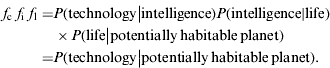
This expression is an estimate of the probability that a technological civilization develops on a potentially habitable planet. All these preliminary remarks and heuristics approaches suggest that equation (1) parameters can be grouped together into two new parameters for which the meaning is straightforward:
1. A=R*f p is the number of new planetary systems produced in the galaxy per year.
2. B=n ef lf if c is the number of advanced intelligent civilizations (AIC) that are able to communicate (and for which we can detect their communication) per planetary systems. AIC can be interpreted as instantiations of the sixth Dick's mega trajectory (Dick Reference Dick2003), in the same way Cirkovic's ATC (i.e. advanced technological civilizations), are instantiations of the seventh one (Cirkovic & Bradbury Reference Cirkovic and Bradbury2006).
In other words, AB is the number of new AIC produced per year. L is the average AIC lifetime. Historically, the Drake equation was rather written N*=Rf sL, where R is the average rate of life-supportable star production, f s is the number of civilizations per suitable star and L is still the average lifetime of an AIC. Equation (1) was established by Shklovsky & Sagan (Reference Shklovsky and Sagan1966) by expanding f s.
AIC appearance occurs in a space that is by definition the galactic habitable zone (GHZ). The concept of GHZ was introduced a few years ago as an extension of the much older concept of Circumstellar Habitable Zone (Lineweaver et al. Reference Lineweaver, Fenner and Gibson2004). This location is usually considered to be an annulus, with an inner radius of 7 kpc and an outer radius of 9 kpc (1 kpc=1000 pc≈3000 light years) (Lineweaver et al. Reference Lineweaver, Fenner and Gibson2004; Forgan Reference Forgan2011). However, other authors are pointing out that the physical processes underlying the former concept are hard to identify and that the entire Milky Way disk may well be suitable for complex life (Prantzos Reference Prantzos2008; Gowanlock et al. Reference Gowanlock, Patton and McConnell2011). In this paper, we will consider the entire Milky Way disk to be suitable for the complex life, i.e. to be the GHZ. This will also allow us to use estimation of R* for the entire galaxy (Diehl et al. Reference Diehl, Halloin, Kretschmer, Lichti, Schönfelder, Strong, von Kienlin, Wang, Jean and Knödlseder2006).
This above new parameter grouping, the need for a temporal structure to the Drake equation and the reasonable assumption that AIC appearance should be roughly random in time and in space (this assumptions are discussed in the following part), strongly suggest that an AIC appearance mathematical model could be made by using a stochastic process like a Poisson process {N(t):t⩾0} with rate parameter λ=AB.
Poisson process
A Poisson process is a continuous-time stochastic process in which events occur continuously and independently of each others. Examples that are well-modelled as Poisson processes include the radioactive decay of atoms (Foata & Fuchs Reference Foata and Fuchs2002), Turing machine rules mutations (Glade et al. Reference Glade, Ben Amor, Bastien and Amar2009), the arrival of customers in a queue n telephone calls arriving at a switchboard and proteins evolution (Bastien Reference Bastien2008; Ortet & Bastien Reference Ortet and Bastien2010). The Poisson process is a collection {N(t):t⩾0} of random variables, where N(t) is the number of events, often called “top”, that have occurred up to time t (starting from time 0). The number of events between time a and time b is given as N(b)−N(a) and has a Poisson distribution. Each realization of the process {N(t):t⩾0} is a non-negative integer-valued step function that is non-decreasing in time. In our case, each “top” could be an AIC appearance. Hence, N(t) would be the number of AIC that has appeared up to time t.
Definition of a homogeneous Poisson process
The homogeneous Poisson process is one of the most well-known Lévy processes (Itô Reference Itô2004). A continuous-time counting process {N(t):t⩾0} will be called a Poisson process if it possesses the following properties:
1. N(0)=0.
2. Independent increments (the numbers of occurrences counted in disjoint intervals are independent from each other).
3. Stationary increments (the probability distribution of the number of occurrences counted in any time interval only depends on the length of the interval).
4. No counted occurrences are simultaneous. More precisely, the process is locally continuous in probability, i.e., for all t⩾0,
 .
 .
In our model, condition 1 means that we must begin the AIC count at a time when no previous AIC exists. Condition 2 means that each AIC evolves independently from each others. Condition 3 means that the number of AIC in a time interval does not depend on the date at which we sample this interval, that is to say invariance of physical law and global homogeneity of the space–time in the considered galaxy region, i.e. the GHZ (Gonzales et al. Reference Gonzalez, Brownlee and Ward2001; Cirkovic Reference Cirkovic2004a, b; Lineweaver et al. Reference Lineweaver, Fenner and Gibson2004; Vukotic & Cirkovic Reference Vukotic and Cirkovic2007; Prantzos Reference Prantzos2008; Gowanlock et al. Reference Gowanlock, Patton and McConnell2011). If these conditions are satisfied, then we can deduce the following results.
1. Consequences of this definition include: The probability distribution of N(t) is a Poisson distribution. That is to say
where N(t+τ)−N(t) is the number of events between the time interval [t, t+τ] and λ is the stochastic process rate parameter also called density or intensity. The product λτ is called the parameter of the Poisson distribution.2. The probability distribution of the waiting time until the next event occurs is an exponential distribution.
3. The occurrences are distributed uniformly on any interval of time. (Note that N(t), the total number of occurrences, has a Poisson distribution over [0, t], whereas the location of an individual occurrence on t in [a, b] is uniform.)
 where N(t+τ)−N(t) is the number of events between the time interval [t, t+τ] and λ is the stochastic process rate parameter also called density or intensity. The product λτ is called the parameter of the Poisson distribution.
Homogeneous and non-homogeneous Poisson process
As recalled above, a homogeneous Poisson process is characterized by its rate parameter λ, which is the expected number of events (also called arrivals) that occur per unit time. Nevertheless, in general, the rate parameter may change over time; such a process is called a non-homogeneous Poisson process or inhomogeneous Poisson process. In this case, the generalized rate function is given as λ(t), where λ(t) is a real continuous function of time (and hence, defined on the positive part of the real axis). In this case, the above definition of a Poisson process remains unchanged except for the third condition (stationary increments). Then, the three Poisson process conditions are:
1. N(0)=0.
2. Independent increments (the numbers of occurrences counted in disjoint intervals are independent from each other).
3. Let
; then for all pair (s,t) with 0⩽s<t<+∞, the number N(t)−N(s) of events occurring in [s, t] is a Poisson random variable with parameter .
 ; then for all pair (s,t) with 0⩽s<t<+∞, the number N(t)−N(s) of events occurring in [s, t] is a Poisson random variable with parameter
![$\mu (\left] {s,t} \right]) = {\rm \rho} (t) - {\rm \rho} (s) = \int_s^t {{\rm \lambda} (u){\rm d}u} $](https://static.cambridge.org/binary/version/id/urn:cambridge.org:id:binary:20151007144341355-0733:S1473550411000413_eqnU5.gif?pub-status=live) .
This last condition implies the fourth of the definition of the homogeneous processes, that is to say: the process is locally continuous in probability. Moreover, it can be demonstrate (Foata & Fuchs Reference Foata and Fuchs2002) that this condition is similar to the following:
Condition 3bis. For h→0, we have P(N(t+h)−N(t)=1)=λ(t)+o(h) and P(N(t+h)−N(t)⩾2)=o(h).
Usually, m(t) is called the renewable function. A remarkable result is that all non-homogeneous Poisson process can be transformed into a homogeneous Poisson process by a time transformation (Foata & Fuchs Reference Foata and Fuchs2002). Of course, a homogeneous Poisson process may be viewed as a special case when λ(t)=λ, a constant rate.
AIC birth and death process
Here, we construct a simple stochastic process that will represent the stochastic appearance of AIC in the Milky Way as a function of time. More exactly, we will construct a model that will give us the number C(t) of existing AIC for a given time t. A first reasonable hypothesis for this model is that there exist a time t 0 for which no AIC is present in the galaxy, i.e. C(t 0)=0. So, without loss of generality, we can consider a stochastic process for which the first condition, C(0)=0, for the process to be a Poisson process is true. A second hypothesis for this model is that AIC appearances (i.e. births) are independent from each other (communication between them does not influence their birth or their lifetime). As a consequence, a possible limitation of the present model could come from the fact that there is a legitimate case to be made that AIC numbers may violate this condition of the Poisson distribution: the longevity, may be significantly affected by the discovery of a long-lived intelligent community, possibly leading to clustering in time. A third hypothesis is that the number of AIC in a time interval does not depend (at least locally) on the date at which we sample this interval.
With these three hypotheses, we can consider the stationary increments Poisson stochastic process {N(t):t⩾0} with density λ>0 (Itô Reference Itô2004) where each “top” of the Poisson process is an AIC birth event. As the rate parameter λ represents the expected number of events that occur per unit time, it is clear that it is equal to the number of new AIC produced per year, that is to say the product AB of the upper new Drake equation parameter grouping. We also suppose that each AIC lifetime is a random variable X, i.e. all AIC during time are independent, identically distributed and are independent of the process {N(t):t⩾0}. Let S k be the birth date of the kth AIC and X k its lifetime. Then, its death date is S k+X k. Let S 0:=X 0:=0 and C(t) be the number of AIC present at the time t. The question is to evaluate the probability law of C(t), with the hypothesis N(0)=0 (and hence C(0)=0). The following theorem for the current AIC number can then be formulated (for the proof, see the Appendix):
Theorem 1.Theorem for the current AIC number: with the previous hypotheses and notations, the number C(t) of AIC present at the time t is a Poisson distributed random variable with parameter  , where λ is the rate parameter of the AIC appearance Poisson stochastic process and r(u) is the survival function of AIC lifetime random variable X.
To resume, the Poisson stochastic process {N(t):t⩾0}, which represents the appearance of new AIC in the Milky Way is combined with a random variable X, which represents the lifetime of these new civilizations. The main result is that the number C(t) of AIC present at time t is a Poisson distributed random variable with parameter m(t). This general result can be link to the classical Drake equation by the following. As t tends to infinity and using a classical theorem of probability about survival function (which stated that  ; Skorokhod & Prokhorov Reference Skorokhod and Prokhorov2004), we observe that
 . As a consequence, C(t) is going towards a Poisson random variable V with parameter λE[X]. This result is exactly the Drake equation with
 , E[X]=L and λ=AB. Interestingly, if one assumes that the lifetime of any galactic civilization is finite, that is to say has an upper bound. Then, their exists a number t M for which r(t M)=0 and so the limit value of m(t) will be reached at finite time, that is to say we will have
 .
Discussion
Mean and variance of the number of AIC
As stated above, as t becomes larger than the AIC maximum lifetime, the previous approximation becomes exact. So we have E[V(t)]=VAR[V(t)]=λE[X] (the mean and the variance of a Poisson distributed random variable are equal; Skorokhod & Prokhorov Reference Skorokhod and Prokhorov2004) and the three terms of the equality are time independent. As a consequence, we can study the coefficient of variation ε of the C(t) (also named fluctuation around the mean) which is the ratio between the SD and the mean of the stochastic process. Here, we have

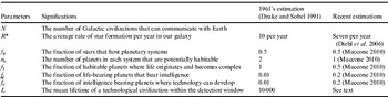
With the 1961's Drake parameters estimation (see Table 1), λ=0.001 and hence, depending on the AIC lifetime, we can have
1. with E[X]=200, we obtain E[V(t)]=0.2 and ε=2.23,
2. with E[X]=10 000, we obtain E[V(t)]=10 and ε=0.31.
An error of magnitude one order in any parameter can lead to a estimation of E[V(t)] and ε equal to 1. For example, a lower bound can be estimated for E[X], while considering the span time between now and the invention of the parabolic telescope, i.e. radioastronomy (Reber & Conklin Reference Reber and Conklin1938). This gives E[X]=73, and so E[V(t)]=0.072 and ε=3.9.
Drake equation parameter estimations

The dramatic effect of parameter evolution estimations on a possible value of N(t) can be seen in the following. Indeed, with more recent estimations (Diehl et al. Reference Diehl, Halloin, Kretschmer, Lichti, Schönfelder, Strong, von Kienlin, Wang, Jean and Knödlseder2006; Maccone Reference Maccone2010), we obtain λ=0.07 and hence, we can have
1. with E[X]=200, we obtain E[V(t)]=14 and ε=0.27,
2. with E[X]=10 000, we obtain E[V(t)]=700 and ε=0.04,
3. with E[X]=73, we obtain E[V(t)]=5 and ε=0.45.
All these considerations give a large probability for detection of another AIC, depending on the reliability of the new estimations. Starting from V(t 0)=0, the Poisson stochastic process theory allow us to estimate the average mean time for the occurrence of a new AIC appearance, which is given by the inverse of λ (Foata & Fuchs Reference Foata and Fuchs2002). With the 1961's Drake parameters estimation (respectively, recent estimation), this average time is equal to 1000 years (respectively, 14 years). Apply to the SETI research programme, if we suppose that we are alone in our universe, the average mean time for the occurrence of another AIC should be roughly 14 years with recent parameter estimations (respectively, 1000 years for the 1961's Drake estimation), with a standard error of the same order error.
Conclusion
The proposed model allows a first analytic estimation of the SD of the number of Galactic civilization estimate. In addition, it provides a temporal structure of the Drake equation which can help study the influence of several effects on the number of Galactic civilization estimate. An important case is the notion of global regulation mechanism (i.e. a dynamical process preventing uniform emergence and development of life all over the Galaxy; Annis Reference Annis1999; Vukotic & Cirkovic Reference Vukotic and Cirkovic2008). Vukotic & Cirkovic (Reference Vukotic and Cirkovic2007) investigated the effects of a particular global regulation mechanism, the Galactic gamma-ray bursts (GRBs) (colossal explosions caused either by terminal collapse of supermassive objects or mergers of binary neutron stars), on the temporal distribution of hypothetical inhabited planets, using simple Monte Carlo numerical experiments. Here, GRB is clearly just one of the possible physical processes for resetting astrobiological clocks. They obtain that the times required for biological evolution on habitable planets of the Milky Way are highly correlated. More precisely, using simulations cosmological observations (Bromm & Loeb Reference Bromm and Loeb2002), they demonstrated that the correlation (and so the covariance cov(t b, t*)) between the biological timescale t b and the astrophysical timescale t* is non-zero. Using the distribution of GRB over the time, an analytic approach would be to compute the random time T since the last GRB event. Assuming that T is independent from both N(t):t⩾0, the Poisson stochastic process that represents the appearance of new AIC, and X which represents the lifetime of these new civilizations, Theorem 1 can be replaced by a more general form:
Theorem 2.Theorem for the current AIC number under global regulation mechanisms: with the previous hypotheses and notations, the number C(T) of AIC present at the time T is a Poisson distributed random variable with parameter  , where λ is the rate parameter of the AIC appearance Poisson stochastic process, r(u) is the survival function of AIC lifetime random variable X and T is the random variable ‘time elapsed since the last major global regulation event’.
This result follows from the above fact that  , which can be rewritten as E[C(T)|T=t]=m(t), where E[.|.] is the conditional expectation operator. This last formula is called the conditional expectation of C given T=t. Since we do not know the true value of t since the last GRB event, we must consider the new random variable m∁T=m(T)=E[C|T]. Future works will explore this result. Especially, it would be suitable to obtain a formula
 where the expectation is computed using the global regulation event (in particular GRB events) distribution over the time. This analytic approach could provide an accurate analysis of classical Monte-Carlo simulations (Vukotic & Cirkovic Reference Vukotic and Cirkovic2008; Forgan Reference Forgan2009, Reference Forgan2011; Hair Reference Hair2011). For instance, Hair (Reference Hair2011) and Forgan (Reference Forgan2011) had proposed in their two models that the distribution of the civilization arrival times is Gaussian-distributed. In principle, this is equivalent to allowing the AIC appearance rate parameter λ, to varying in time. More precisely, the rate parameter λ(t) corresponding to the Forgan model (Forgan Reference Forgan2011) should be an increasing function of [0, μ], where μ is the mean of the Hair (Reference Hair2011) and Forgan (Reference Forgan2011) arrival time Gaussian distribution (μ has the same order of magnitude than the Hubble time, t H=13 700 Myr), and a decreasing function of [μ, +∞]. Nevertheless, this work is mainly the first approach to model AIC appearance, but future studies would have to address the fact that AIC appearance in habitable planets should be correlated with the Galaxy's star formation history (Heavens et al. Reference Heavens, Panter, Jimenez and Dunlop2004; Juneau et al. Reference Juneau, Glazebrook, Crampton, McCarthy, Savaglio, Abraham, Carlberg, Chen, Borgne and Marzke2005; Vukotic & Cirkovic Reference Vukotic and Cirkovic2007) and the location of the GHZ (Gonzalez et al. Reference Gonzalez, Brownlee and Ward2001; Lineweaver et al. Reference Lineweaver, Fenner and Gibson2004; Prantzos Reference Prantzos2008; Gowanlock et al. Reference Gowanlock, Patton and McConnell2011). For instance, Planet formation and star formation could be included in the first AIC appearance model by extracting the original Drake parameters R*, f p and n e from λ and let them to vary in time.
Appendix: Demonstration of the theorem
The proof of the theorem can be divided into three parts (Foata & Fuchs Reference Foata and Fuchs2002).
Lemma 1.Let r(u):=P{X⩾u} be the survival function of X and 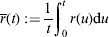 . If U is a uniform random variable on [0, t], independent of X, the survival function of U+X is given by
 .
Proof. Following the fact that the density of U is ![${\textstyle{1 \over t}}I_{[0,t[} $](https://static.cambridge.org/binary/version/id/urn:cambridge.org:id:binary:20151007144341355-0733:S1473550411000413_eqnU17.gif?pub-status=live) , where
![$I_{[0,t[} (x)$](https://static.cambridge.org/binary/version/id/urn:cambridge.org:id:binary:20151007144341355-0733:S1473550411000413_eqnU18.gif?pub-status=live) is 0 outside the interval [0,t[, we have
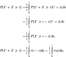
which are equal to  by definition.
Lemma 2.The generating function h(u):=E[uC (t)] of C(t) is given by  .
Proof. For k⩾0, let  . Obviously we have
 , and so
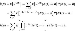
Conditionally to the event {N(t)=n} (n⩾1), the system (S 1,S 2, … ,S n) has the same distribution than the system (U 1,U 2, … ,U n) of independent and uniformly distributed on [0, t] random variables.
For 1⩽k⩽n, let Z k:=I {Uk+Xk⩾t}. We have

But Z 1 is a Bernoulli random variable with parameter  . Hence,
 is the generating function of the Z 1 random variable and is given by
 (Koroliouk Reference Koroliouk1978). Finally, we obtain

Proof of the theorem. We can write 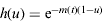 which is the generating function of a composed Poisson distribution (Koroliouk Reference Koroliouk1978) and so, is a Poisson distributed random variable with parameter

Acknowledgements
O.B. was supported by the French Agence Nationale de la Recherche, as part of the ReGal project.
Author disclosure statement
No competing financial interests exist.