


1. Introduction
The accurate modeling of mortality risk plays a fundamental role in the insurance and pension industries, where the valuation and risk management of financial instruments are intricately tied to demographic uncertainties. Mortality-linked securities, such as longevity bonds and catastrophe mortality bonds, serve as vital tools for transferring risk from insurers to the capital markets. These instruments enable stakeholders to manage exposure to extreme demographic events while supporting the stability of financial systems. However, the development of these securities requires sophisticated models that account for the stochastic dynamics of mortality rates and their interplay with economic variables, particularly interest rates as their joint behavior determines the valuation of mortality-linked securities (Biffis, Reference Biffis2005; Blackburn and Sherris, Reference Blackburn and Sherris2013).
Traditional approaches to mortality modeling often rely on deterministic methods, such as life tables or parametric laws (e.g., Gompertz, Reference Gompertz1825; Makeham, Reference Makeham1860). While these models provide useful baselines for life insurance pricing, they fail to capture the inherent randomness and temporal evolution of mortality rates, especially in the face of systemic demographic shocks. To address these limitations, stochastic mortality models have been developed, such as the Lee–Carter model (Lee and Carter, Reference Lee and Carter1992) and the Cairns–Blake–Dowd models (Cairns et al., Reference Cairns, Blake and Dowd2006; Cairns et al., Reference Cairns, Blake, Dowd, Coughlan, Epstein, Ong and Balevich2009). These seminal works introduced discrete-time stochastic frameworks for mortality forecasting, which have since been extended to continuous-time settings (Biffis, Reference Biffis2005; Blackburn and Sherris, Reference Blackburn and Sherris2013). Such stochastic approaches offer more robust tools for assessing demographic risks over time and are particularly relevant when mortality is coupled with economic factors, such as fluctuating interest rates, which jointly influence the valuation of mortality-linked securities (Milevsky and Promislow, Reference Milevsky and Promislow2001; Zeddouk and Devolder, Reference Zeddouk and Devolder2020).
A rich body of work has addressed mortality modeling and the pricing of longevity-linked securities through the lens of affine frameworks and contingent-claim analysis. For example, Bauer and Kramer (Reference Bauer and Kramer2016) employ a continuous-time approach to quantify the risk of mortality catastrophes, showing that extreme mortality events can be priced within a no-arbitrage framework. Affine mortality modeling has been developed by Jevtić et al. (Reference Jevtić, Luciano and Vigna2013) who construct a continuous-time cohort model for the mortality surface, Blackburn and Sherris (Reference Blackburn and Sherris2013) who propose a Heath-Jarrow-Morton framework for mortality, and Jevtić and Regis (Reference Jevtić and Regis2019) who extend the continuous-time stochastic approach to multiple populations. More recently, Hanna and Devolder (Reference Hanna and Devolder2024) develop a multidimensional affine approach using Hull–White dynamics for interest and mortality rates. Ungolo et al. (Reference Ungolo, Garces, Sherris and Zhou2024) conduct a systematic comparison of multifactor affine mortality models, and Ungolo et al. (Reference Ungolo, Garces, Sherris and Zhou2025) operationalize a broad library of affine specifications in an open-source R package.
While these affine mortality studies have substantially advanced the field, a common limitation is the reliance on standard Brownian motion as the driving noise, which precludes LRD in the dynamics of mortality and interest rates. Empirical evidence based on real-world data suggests that both mortality and interest rates exhibit LRD, characterized by persistent correlations over extended time horizons (Cajueiro and Tabak, Reference Cajueiro and Tabak2007; Wang et al., Reference Wang, Chiu and Wong2021; Yan et al., Reference Yan, Peters and Chan2019). Recent actuarial studies, such as Yan et al. (Reference Yan, Peters and Chan2021), Zhou et al. (Reference Zhou, Zhou and Li2022), Zhou and Li (Reference Zhou and Li2023), Deelstra et al. (Reference Deelstra, Devolder and Roelants du Vivier2024), have investigated the importance of LRD in mortality modeling and demonstrated its critical role in accurately pricing longevity-linked securities and life insurance products. In particular, frameworks based on fractional Ornstein–Uhlenbeck processes (Delgado-Vences and Ornelas, Reference Delgado-Vences and Ornelas2019) and mixed fractional Poisson processes (Jiang et al., Reference Jiang, Zhang and Zhu2024), have been developed to capture these effects, providing a theoretical basis for incorporating long-memory dynamics.
Another key limitation is the lack of joint modeling of mortality and interest, as unexpected shocks can simultaneously affect mortality and interest rate trajectories. For instance, the COVID-19 pandemic triggered sharp spikes in mortality from direct health impacts, while central banks responded with aggressive monetary easing that depressed long-term interest rates. Conversely, a financial crisis may primarily affect interest rates through market stress, while also having indirect effects on mortality through reduced healthcare spending. Many existing mortality models fail to capture such systemic shocks when accounting for long-memory features. This interdependence further complicates the pricing process of mortality-linked products (Deelstra et al., Reference Deelstra, Devolder and Roelants du Vivier2024; Hanna and Devolder, Reference Hanna and Devolder2024) and motivates the need for a joint modeling framework that integrates LRD, short-term volatility, mean-reverting trends, and instantaneous correlation.
This paper introduces a novel bivariate stochastic framework to jointly model excess mortality and interest rate dynamics. We focus on excess mortality rather than raw mortality, as the latter exhibit seasonal variation that would otherwise require explicit modeling. The mixed fractional Brownian motion that drives our stochastic model can effectively capture the LRD inherent in both mortality and interest rate data. The drift part of our model incorporates mean-reverting trends that are essential for pricing mortality-linked securities. The model also considers short-term volatility and explicitly uses a correlation coefficient matrix to describe the interactions between mortality and interest rates. By addressing these interdependencies and dynamic features, our model framework aims to overcome limitations in existing stochastic mortality models and provide a robust foundation for actuarial and financial applications.
A key modeling choice in our framework is to work with excess mortality rather than raw (all-cause) mortality rates. Excess mortality is defined as the deviation of the observed mortality rate from a pre-specified baseline that reflects normal seasonal and trend patterns. This has two important advantages for our purposes. First, it removes predictable seasonal variation (e.g., higher winter mortality) that would otherwise need to be modeled through a separate seasonal component, keeping the stochastic model parsimonious. Second, the resulting series fluctuates around zero in normal times and exhibits positive spikes during periods of elevated mortality – such as pandemics, heatwaves, or other catastrophic events – making it a natural candidate for the mean-reverting Vasicek-type specification we employ. This approach is consistent with recent work on pandemic-era mortality modeling (e.g., Li et al., Reference Li, Liu, Tang and Yuan2023) and aligns with the data structure of the HMD Short-Term Mortality Fluctuations database, which provides the weekly observations used in our empirical analysis.
The contributions of this paper are threefold. The first goal of this paper is to contribute in the research line on the applications of fractional Brownian motion in actuarial work and to explore the valuable insights that fractional models can offer to capture the joint dynamics of interest rate and mortality rate. As mentioned, a novel long-memory bivariate stochastic framework driven by a flexible long-memory process, mixed fractional Brownian motion, is proposed and studied. Fractional Brownian motion is known to have more flexibility than Brownian motion that has been traditionally used in actuarial literature. It can effectively capture the LRD that has been proved to exist in financial market and mortality data. Due to the tractability challenges that classic Itô calculus cannot be directly applied in stochastic models driven by fractional Brownian motion, the research on these models still remains a frontier in probability theory, and it also appears to be an emerging field in applications including both quantitative finance and actuarial science. Through our investigation in this paper, the model we present demonstrates another important application of fractional Brownian motion in actuarial work. It has sufficient flexibility to capture the fore-mentioned features to fill significant gaps in the actuarial literature of stochastic modeling and provides a robust tool for analyzing mortality-interest rate dynamics.
Second, we study the properties of the proposed model, including the probabilities of negative interest rates, the upper and lower bound estimates for the tail probability of extreme mortality rates, and the representation of the model under a risk-neutral pricing measure. Based on these properties, we derive analytical solutions for pricing financial instruments, such as zero-coupon bonds and catastrophe mortality bonds. Specifically, we obtain the value of zero-coupon bonds both at the time of issuance and at any subsequent time point during their lifetime. Furthermore, we investigate the application of the proposed model to price catastrophe mortality bonds, extending its utility to manage extreme mortality risks, similar to the ones considered in Chen et al. (Reference Chen, Yang and Huang2022) and Schmitt and Spaeter (Reference Schmitt and Spaeter2023). These analytical solutions enhance the tractability of the model and provide valuable tools for actuarial and financial applications.
Third, the paper presents a comprehensive calibration methodology using weekly mortality data from the Short-Term Mortality Fluctuations series of the Human Mortality Database (HMD) and interest rate data from the Federal Reserve Economic Data (FRED). It should be mentioned that our framework models excess mortality rates, which provides flexibility in the choice of baseline mortality. While Li et al. (Reference Li, Liu, Tang and Yuan2023) adopts average mortality rates over the observation period as the baseline, we take a different approach that accounts for seasonality in weekly mortality patterns and allows for adaptability to potential systemic shifts in mortality dynamics. A sequential calibration procedure is designed to estimate the parameters of the proposed bivariate model, including long-memory Hurst parameters to quantify long-term persistence and the correlation coefficient between mortality and interest rates. Numerical results reveal, similar to findings in Li et al. (Reference Li, Liu, Tang and Yuan2023), that the correlation between mortality and interest rates is negative. Additionally, the proposed model is calibrated under the pricing measure to observed real-world catastrophe mortality bond prices, demonstrating its practical applicability for risk management and insurance pricing.
The paper is organized as follows. In Section 2, the stochastic calculus elements concerning the fractional Brownian motion and the mixed fractional Brownian motion are introduced. In Section 3, we propose our bivariate stochastic models to describe the joint dynamics of interest rates and excess mortality rates. The properties of the proposed model will be studied that include an estimate of the extreme value of excess mortality and the construction of the pricing measure
 $\mathbb{Q}$
. In Section 4, actuarial mathematics is developed with respect to the pricing of mortality-linked securities. In Section 5, we will discuss the methodologies of calibrating our stochastic models under both physical measure
 $\mathbb{P}$
and pricing measure
 $\mathbb{Q}$
. The simulation-based numerical analysis is applied in Section 6 to investigate the sensitivity of a stylized catastrophic mortality bond to the changes in different parameters of our stochastic models. We conclude the paper in Section 7 by summarizing our main results and discussing potential future work.
2. Stochastic calculus elements
As the fractional Brownian motion (fBm) is not Markovian, the classic Itô calculus cannot be directly applied to study the stochastic integrals with respect to fBm. In this section, we introduce some important elements of stochastic analysis that we will use to analyze the properties of stochastic models driven by fractional Brownian motion.
2.1. Fractional Brownian motion
We consider a filtered probability space
 $(\Omega, \mathcal{F}, \mathcal{F}_t, \mathbb{P})$
such that all random variables are well defined and stochastic processes are
 $\mathcal{F}_t$
adapted. The natural filtration of a stochastic process is taken as the
 $\mathbb{P}$
-completion of the filtration that it generates. For some fixed
 $T\gt0$
, a (standard) fractional Brownian motion (fBm) on time interval [0, T],
 $B^H = (B_t^H, t \in [0, T])$
with Hurst parameter
 $H \in (0, 1)$
is defined as a centered Gaussian process with continuous paths such that
 $B_0^H = 0$
and
 \begin{align*}\mathrm{Cov}(B^H_s, B^H_t) = \mathbb{E}\left(B^H_s B^H_t\right) = \frac{1}{2}\left(s^{2H} + t^{2H} - |s-t|^{2H}\right), \ 0 \leq s, t \leq T. \end{align*}
The Hurst parameter
 $H \in (0,1)$
governs the memory structure of the fBm and has a direct economic interpretation. When
 $H = \tfrac{1}{2}$
, the fBm reduces to standard Brownian motion, where increments are independent and the process has no memory of past shocks. When
 $H \gt \tfrac{1}{2}$
, the process exhibits LRD. In the context of excess mortality,
 $H \gt \tfrac{1}{2}$
captures the phenomenon whereby a mortality shock persists over many periods rather than reverting quickly, such as the lasting effect of the COVID-19 pandemic. For interest rates,
 $H \gt \tfrac{1}{2}$
reflects prolonged monetary-policy regimes, such as the low interest rate periods observed over 2008–2015 and 2020–2021. Conversely, when
 $H \lt \tfrac{1}{2}$
, the process is antipersistent, meaning that positive increments tend to be followed by negative corrections. This will produce rougher and more rapidly mean-reverting trajectories that may be relevant for short-term fluctuations that are quickly corrected by market forces. Lastly, we remark that, when
 $H \neq \frac{1}{2}$
, fBm is not a semimartingale and the classic Itô theory cannot be applied to study the corresponding stochastic integrals.
The construction of stochastic integrals can follow the traditional limiting arguments (see Hu et al., Reference Hu, Nualart and Zhou2019; Nualart, Reference Nualart2006 and the references therein). Specifically, we consider the elementary space
 $\mathcal{E}$
of real valued step functions and define the Hilbert space
 $\mathfrak{H}$
as the closure of the space
 $\mathcal{E}$
endowed with the inner product
 \begin{align*} \langle \unicode{x1D7D9}_{[0, t]}, \unicode{x1D7D9}_{[0, s]} \rangle_{\mathfrak{H}} = \mathbb{E}(B_s^H B_t^H). \end{align*}
The mapping
 $\unicode{x1D7D9}_{[0, t]} \to B_t^H$
can be extended to the linear isometry between the Hilbert space and the Gaussian subspace spanned by fBm. In other words,
 $\int_0^T \unicode{x1D7D9}_{[0, t]} (s) dB_s^H = B^H_t$
. By the limiting argument, the stochastic integral (also called the Wiener integral)
 $ \int_0^T f(t) dB_t^H$
whose integrand
 $f \in \mathfrak{H}$
is deterministic follows a centered Gaussian distribution. When
 $H\gt\frac{1}{2}$
, the variance can be computed by
 \begin{equation} \mathbb{E}\left[\left(\int_0^T f(t) dB_t^H\right)^2\right] = \alpha_H \int_0^T \int_0^T f(s) f(t) |t-s|^{2H-2} {\mathop{}\! {\mathop{}\!\mathrm{d}}s{\mathop{}\!\mathrm{d}}t}, \end{equation}
where
 $\alpha_H = H(2H-1)$
. The covariance between two Wiener integrals is computed by
 \begin{equation} \mathrm{Cov}\left(\int_0^T f(t) dB_t^H, \int_0^T g(t) dB_t^H\right) = \alpha_H\int_0^T \int_0^T f(t) g(s) |t-s|^{2H-2} {\mathop{}\! {\mathop{}\!\mathrm{d}}s{\mathop{}\!\mathrm{d}}t}. \end{equation}
There are some integral transformations that can change fBm to martingales (see Norros et al., Reference Norros, Valkeila and Virtamo1999). The following results from Norros et al. (Reference Norros, Valkeila and Virtamo1999) will be used in this paper. We first introduce the deterministic functions for
 $0 \lt s \lt t \leq T$
,
 \begin{align*}k_H(t, s) = \kappa_H^{-1} s^{\frac{1}{2} - H} (t-s)^{\frac{1}{2} - H}, \ \kappa_H = 2H\Gamma\bigg(\frac{3}{2}-H\bigg)\Gamma\bigg(H+\frac{1}{2}\bigg), \end{align*}
 \begin{align*}\omega_t^H = \lambda_H^{-1} t^{2-2H}, \ \lambda_H = \frac{2H\Gamma(3-2H)\Gamma(H+\frac{1}{2})}{\Gamma(\frac{3}{2}-H)}. \end{align*}
Then, we can construct a Gaussian martingale
 $M_t^H = \int_0^t k_H(t, s) dB_s^H$
, and it is called the fundamental martingale. The natural filtration generated by this martingale actually coincides with that of the fBm
 $B^H$
, and the quadratic variation
 $\langle M^H \rangle_t$
equals
 $\omega_t^H$
. The fundamental martingale is very useful in the stochastic analysis about fBm, and one of the applications is to derive the Girsanov formula for fBm (see Kleptsyna et al., Reference Kleptsyna, Breton and Roubaud2000). Namely, we consider a process
 $Y_t$
that is the pathwise solution to the following stochastic differential equation
 \begin{align*}dY_t = A(t) dt + \sigma(t) dB_t^H, \ 0 \leq t \leq T, \end{align*}
where the functions
 $A(t), \sigma(t)$
satisfy some nice properties to ensure the existence of a pathwise solution for a given initial condition. The process defined by
 \begin{align*}Q_H(t) = \frac{d}{d \omega_t^H} \int_0^t k_H(t, s)\sigma^{-1}(s)A(s) {\mathop{}\! {\mathop{}\!\mathrm{d}}s}, \ t \in [0, T], \end{align*}
belongs to the measurable space
 $L^2([0, T], d\omega^H)$
. Then, we can construct the random variable
 \begin{align*}Z_H(T) = \exp\left(-\int_0^T Q_H(t) dM_t^H - \frac{1}{2} \int_0^T (Q_H(t))^2 d\omega_t^H\right) \end{align*}
such that
 $\mathbb{E}[Z_H(T)] = 1$
. Consequently,
 $\mathbb{Q} = Z(T)\mathbb{P}$
is a probability measure, and the process Y under the measure
 $\mathbb{Q}$
satisfies the following equation
 \begin{align*}dY_t = \sigma(t) dB_t^{H, \mathbb{Q}}, \ t \in [0, T], \end{align*}
where
 $B_t^{H, \mathbb{Q}}$
is a fBm with Hurst parameter H under measure
 $\mathbb{Q}$
.
2.2. Mixed fractional Brownian motion
We will use the combination of fBm and Bm for our proposed stochastic models, as it offers the flexibility of describing different types of driving noise. A mixed fractional Brownian motion (mfBm),
 $B = B^{\alpha, H} = \{B_t, t \in [0, T]\}$
with parameters
 $\alpha$
and H, was first introduced in Cheridito (Reference Cheridito2001). It is defined as
 \begin{equation} B_t = \alpha W_t + B_t^H,\end{equation}
where
 $\{W_t, t \in [0, T]\}$
is a standard Brownian motion,
 $\{B_t^H, t \in [0, T]\}$
is a fBm with Hurst parameter H, and these two processes are assumed to be independent. The parameter
 $\alpha \in \mathbb{R}^+$
governs the relative contribution of the standard Brownian component to the mfBm.
The two processes underlying the mfBm in Equation (3) have distinct economic roles in mortality and interest rate modeling. The standard Bm captures short-lived, memoryless shocks; for example, transitory weather-related mortality fluctuations or short-term liquidity-driven movements in the money market. By contrast, the fBm captures persistent dynamics; for example, the gradual and sustained impact of pandemics and the slow build-up and unwinding of inflation expectations that shape long-term interest rate movements. By combining both components, the mfBm offers the flexibility to control the relative contribution of short-memory and long-memory effects within a single unified setup.
An mfBm inherits many properties from the fBm. It is not a semimartingale if
 $H \neq \frac{1}{2}$
. When
 $H=\frac{1}{2}$
, the mfBm is essentially a Bm. When
 $H \in (\frac{1}{2}, 1)$
, the increment of mfBm exhibits long-range dependence (LRD). Namely, we can take a look at the correlation of the increments. Since the mfBm has stationary increments, we can compute
 \begin{align*}\rho(k) \, :\!= \, \mathbb{E}[B_1(B_{k+1} - B_k)] = \frac{1}{2}[(k+1)^{2H} - 2k^{2H} + (k-1)^{2H}], \end{align*}
for any natural number
 $k \geq 1$
. Clearly, when k is large, the correlation
 $\rho(k)$
behaves like
 $k^{2H-2}$
and
 $\sum_k \rho(k) = \infty$
when
 $H \gt \frac{1}{2}$
. This shows that the mfBm has LRD when
 $H \gt \frac{1}{2}$
.
To model the joint dynamics of interest rate and mortality rate under the influence of both temporary and persistent effect, it is natural to consider the use of mfBm. On the one hand, standard Bm is commonly employed to capture short-term stochastic fluctuations arising from the economic and ecological environment. On the other hand, there is growing empirical evidence that mortality rates and economic data exhibit long-memory behavior, as documented in Zhou et al. (Reference Zhou, Zhou and Li2022) and references therein. The LRD reflects the persistent impact of sociodemographic, medical, and environmental factors over extended periods. Similarly, studies such as Li et al. (Reference Li, Liu, Tang and Yuan2023) have shown interest rates, under stressed conditions, exhibit sensitivity to health-related shocks. They do not necessarily imply a direct causal relationship but they reveal meaningful empirical association. As noted, the COVID-19 pandemic has reinforced this interdependence and highlighted how systemic events can induce lasting correlated shifts in both financial market and human mortality. These observations suggest a modeling framework based on mfBm, in contrast to traditional Brownian models, offers a more realistic and flexible approach for capturing the joint behavior of interest rates and mortality rates. In the next section, we introduce a general version of this framework and present its mathematical formulation.
3. Model description
In this section, we propose a bivariate stochastic model for interest rate process and excess mortality process. Specifically, each process is modeled as a Vasicek-type stochastic differential equation driven by a mfBm. The two processes are linked through a correlated structure governed by an instantaneous correlation parameter. We then derive the key distributional properties of this bivariate model, which serve as the foundation for the numerical analysis in subsequent sections.
Assume that the bivariate process
 $\{ X_t, 0 \leq t \leq T \}$
follows a mean-reverting process. Namely, for any
 $0 \leq t \leq T$
,
 \begin{align*}dX_t = (m_t - \Theta_t X_t)dt + \Sigma_{1,t} A_t dW_t + \Sigma_{2,t} dB_t^H, \end{align*}
where
 $\Theta_t, \Sigma_{1,t}, \Sigma_{2,t}, A_t \in \mathbb{R}^{2 \times 2}$
, and
 $m_t \in \mathbb{R}^2$
are all deterministic functions of t.
 $W_t = (W_{1, t}, W_{2, t})'$
for
 $0 \leq t \leq T$
is a standard bivariate Brownian motion.
 $B_t^H = (B_{1, t}^{H_1}, B_{2, t}^{H_2})'$
for
 $0 \leq t \leq T$
is a bivariate fractional Brownian motion with Hurst parameters
 $H = (H_1, H_2) \in (\frac{1}{2}, 1) \times (\frac{1}{2}, 1)$
. We assume that the stochastic process
 $W_t$
is independent of
 $B_t$
.
By taking
 \begin{align*}\Theta_t = \left(\begin{matrix} \theta_1 &\quad 0 \\[3pt] 0 &\quad \theta_2 \end{matrix}\right), \ m_t = \left(\begin{matrix} m_1 \\[3pt] m_2 \end{matrix} \right), \ A_t = \left(\begin{matrix} \alpha_1 &\quad 0 \\[3pt] 0 &\quad \alpha_2 \end{matrix}\right), \ \Sigma_{1,t} = \left(\begin{matrix} \sigma_1 &\quad 0 \\[3pt] \frac{\sigma_2 \alpha_2}{\alpha_1} \rho &\quad \sigma_2 \sqrt{1-\rho^2}\end{matrix}\right), \ \Sigma_{2,t} = \left(\begin{matrix} \sigma_1 & 0 \\[3pt] 0 &\quad \sigma_2 \end{matrix}\right), \end{align*}
we can consider an important special case to model the interest rate process
 $r_t$
and the excess mortality process
 $\mu_t$
. Equivalently, the bivariate process
 $(r_t, \mu_t)'$
satisfies the system of stochastic differential equations (SDEs),
 \begin{eqnarray} d r_t & = & (m_1 - \theta_1 r_t) dt + \sigma_1 (\alpha_1 dW_{1, t} + d B_{1, t}^{H_1}), \nonumber\\[3pt] d \mu_t & = & (m_2 - \theta_2 \mu_t) dt + \sigma_2 \left[\alpha_2 \left(\rho dW_{1, t} + \sqrt{1-\rho^2} dW_{2, t} \right) + d B_{2, t}^{H_2}\right]. \end{eqnarray}
This is essentially a Vasicek-type model, where
 $\theta_1$
and
 $\theta_2$
are the speed of mean reversion,
 $m_1$
and
 $m_2$
are the drift parameters,
 $\sigma_1$
and
 $\sigma_2$
are the volatility parameters, and
 $\rho$
is the correlation parameter.
The mean-reverting dynamics of
 $r_t$
and
 $\mu_t$
are governed by their respective parameters
 $(\theta_1, m_1)$
and
 $(\theta_2, m_2)$
independently. The long-term mean of
 $r_t$
is given by
 $\bar{r} \, :\!= \, m_1 / \theta_1$
, while the long-term mean of
 $\mu_t$
is given by
 $\bar{\mu} \, :\!= \, m_2 / \theta_2$
. A rapid mean reversion of
 $\mu_t$
(i.e., large
 $\theta_2$
) does not necessarily affect the long-term mean of
 $r_t$
(i.e., change
 $\bar{r}$
), and vice versa. The dependence between
 $r_t$
and
 $\mu_t$
is captured specifically by the correlation parameter
 $\rho$
. This instantaneous correlation between the two processes can be computed using the following lemma.
Lemma 3.1. Suppose the interest rate
 $r_t$
and excess mortality rate
 $\mu_t$
are described by the system of SDEs (4). For
 $H \in (\frac{1}{2}, 1)$
, the instantaneous covariance of the increments is given by
 \begin{align*}\mathrm{Cov}(d r_t, d \mu_t) = \rho \sigma_1 \sigma_2 \alpha_1 \alpha_2 {\mathop{}\! {\mathop{}\!\mathrm{d}}t} \end{align*}
and the instantaneous correlation is given by
 \begin{align*}\mathrm{Corr}(d r_t, d \mu_t) \approx \frac{\rho \sigma_1 \sigma_2 \alpha_1 \alpha_2 {\mathop{}\! {\mathop{}\!\mathrm{d}}t}}{\sqrt{\sigma_1^2 \alpha_1^2 {\mathop{}\! {\mathop{}\!\mathrm{d}}t} + \sigma_1^2 ({\mathop{}\! {\mathop{}\!\mathrm{d}}t})^{2H_1}}\sqrt{\sigma_2^2 \alpha_2^2 {\mathop{}\! {\mathop{}\!\mathrm{d}}t} + \sigma_2^2 ({\mathop{}\! {\mathop{}\!\mathrm{d}}t})^{2H_2}}}. \end{align*}
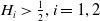
The instantaneous correlation given in Lemma 3.1 demonstrates that Hurst parameters
 $H_1$
and
 $H_2$
affect the instantaneous correlation between the interest rate and the excess mortality rate when observed over a small time interval. Specifically, while the instantaneous covariance arising from the correlated Brownian motions is proportional to the time increment dt, the instantaneous correlation relates to dt through the variance terms, which contain contributions from both the Brownian and fractional Brownian components. As the time increment dt approaches zero when
 $H_i \gt \frac{1}{2}, i=1, 2$
, the instantaneous correlation will approach
 $\rho$
. However, for small dt, the fractional Brownian motion inflates the variances, which tends to reduce the magnitude of the correlation compared to
 $\rho$
.
In the next two theorems, we discuss the positiveness of interest rates and an estimate of extreme mortality rates. We will use the function
 \begin{align*}\nu_t^2(\alpha, H, \theta, \sigma) = \frac{\alpha^2 \sigma^2 \left(1 - e^{-2\theta t}\right)}{2\theta} + \frac{\sigma^2 H(2H-1)}{\theta^{2H} } \left(\gamma(2H-1, \theta t) - e^{-\theta_1 t} \gamma^*(2H-1, \theta t)\right), \end{align*}
where the incomplete gamma functions are given by
 \begin{align*}\gamma(u, x) = \int_0^x s^{u-1} e^{-s} {\mathop{}\! {\mathop{}\!\mathrm{d}}s}, \quad \gamma^*(u, x) = \int_0^x (x-s)^{u-1} e^{-s} {\mathop{}\! {\mathop{}\!\mathrm{d}}s}. \end{align*}
Theorem 3.2. Suppose that the interest rate
 $r_t$
is described by the system of SDEs (4). Then, the random variable
 $r_t$
follows the normal distribution with mean
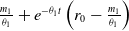 $\frac{m_1}{\theta_1} + e^{-\theta_1 t}\left(r_0 - \frac{m_1}{\theta_1}\right)$
and variance
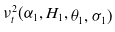 $\nu_t^2(\alpha_1, H_1, \theta_1, \sigma_1)$
. In addition, the probability that
 $r_t$
is nonnegative is given by
 \begin{equation} P(r_t \geq 0) = \Phi\left(\frac{\frac{m_1}{\theta_1} + e^{-\theta_1 t}\left(r_0 - \frac{m_1}{\theta_1}\right)}{\nu_t(\alpha_1, H_1, \theta_1, \sigma_1)}\right), \end{equation}
where
 $\Phi(\! \cdot \!)$
denotes the cumulative distribution function of the standard normal distribution.
Proof. The pathwise solution to the SDE for
 $r_t$
with initial condition
 $r_0$
is
 \begin{align*}r_t = \frac{m_1}{\theta_1} + e^{-\theta_1 t}\left(r_0 - \frac{m_1}{\theta_1}\right) + \sigma_1 \int_0^t e^{-\theta_1(t-s)} d(\alpha_1 W_{1,s} + B_{1,s}^{H_1}). \end{align*}
Clearly, it is a Gaussian random variable with mean
 $\frac{m_1}{\theta_1} + e^{-\theta_1 t}\left(r_0 - \frac{m_1}{\theta_1}\right)$
according to the property of stochastic integrals (Mishura, Reference Mishura2008; Biagini et al., Reference Biagini, Hu, Øksendal and Zhang2008). To compute the variance, we use the formula (1) to derive
 \begin{eqnarray*} \mathrm{Var}[r_t] & = & \mathrm{Var}\left[\sigma_1 e^{-\theta_1 t} \left(\int_0^t \alpha_1 e^{\theta_1 s} dW_{1,s} + \int_0^t e^{\theta_1 s} dB_{1, s}^{H_1}\right)\right] \\[3pt] & = & \sigma_1^2 e^{-2\theta_1 t} \left(\alpha_1^2 \int_0^t e^{2\theta_1 s} {\mathop{}\! {\mathop{}\!\mathrm{d}}s} + H_1(2H_1-1)\int_0^t \int_0^t e^{\theta_1 (u+v)} |u-v|^{2H_1-2} {\mathop{}\! {\mathop{}\!\mathrm{d}}u}{\mathop{}\! {\mathop{}\!\mathrm{d}}v}\right) \\[3pt] & = & \frac{\alpha_1^2 \sigma_1^2 \left(1 - e^{-2\theta_1 t}\right)}{2\theta_1} + \frac{\sigma_1^2 H_1(2H_1-1)}{\theta_1^{2H_1}} \left(\int_0^{\theta_1 t} e^{-x} x^{2H_1-2} {\mathop{}\! {\mathop{}\!\mathrm{d}}x} - \int_0^{\theta_1 t} e^{-2\theta_1 t + x} x^{2H_1-2} {\mathop{}\! {\mathop{}\!\mathrm{d}}x}\right), \\[-30pt] \end{eqnarray*}
where we have made change of variables
 $x=\theta_1(u-v)$
,
 $y=\theta_1 v$
when evaluating the double integral. As
 $r_t$
is Gaussian, it is clear that
 \begin{align*}P(r_t \geq 0) = \Phi\left(\frac{\frac{m_1}{\theta_1} + e^{-\theta_1 t}\left(r_0 - \frac{m_1}{\theta_1}\right)}{\sqrt{\frac{\alpha_1^2 \sigma_1^2 \left(1 - e^{-2\theta_1 t}\right)}{2\theta_1}} + \frac{\sigma_1^2 H_1(2H_1-1)}{\theta_1^{2H_1}} \left(\gamma(2H_1-1, \theta_1 t) - e^{-\theta_1 t} \gamma^*(2H_1-1, \theta_1 t)\right)} \right), \end{align*}
which is consistent with (5).
The variance function
 $\nu_t^2$
is an increasing function of time t. It should be noted that as
 $t \to \infty$
, we have
 \begin{align*}\lim_{t \to \infty} \nu_t^2 = \frac{\alpha_1^2 \sigma_1^2}{2\theta_1} + \frac{\sigma_1^2 \Gamma(2H_1+1)}{2\theta_1^{2H_1}}, \end{align*}
and moreover, when t is large,
 \begin{align*}P(r_t \geq 0) \approx \Phi\left(\frac{\frac{m_1}{\theta_1}}{\sqrt{\frac{\alpha_1^2 \sigma_1^2}{2\theta_1} + \frac{\sigma_1^2 \Gamma(2H_1+1)}{2\theta_1^{2H_1}}}}\right) = \Phi\left(\sqrt{\frac{2m_1^2}{\alpha_1^2 \sigma_1^2 \theta_1 + \sigma_1^2 \Gamma(2H_1+1)\theta_1^{2-2H_1}}}\right). \end{align*}
It is well known that the Gaussian specification of
 $r_t$
in the Vasicek framework does not prevent negative interest rates in theory (see, e.g., Brigo and Mercurio, Reference Brigo and Mercurio2006). However, for the parameter values calibrated in Section 6, the probability of
 $r_t$
becoming negative is negligibly small over the time horizons relevant to our applications.
Similarly, we can see that the excess mortality rate
 $\mu_t$
given by (4) is also a Gaussian process with mean
 $\mathbb{E}[\mu_t] = \frac{m_2}{\theta_2} + e^{-\theta_2 t}\left(\mu_0 - \frac{m_2}{\theta_2}\right)$
and variance
 $\mathrm{Var}[\mu_t] = \nu_t^2(\alpha_2, H_2, \theta_2, \sigma_2)$
. Using properties of Gaussian processes, we can find an upper and a lower bound for the tail probability of extreme excess mortality rates in the time interval [0, T]. This is stated in the following theorem.
Theorem 3.3. The maximum value of the excess mortality rate
 $\mu_t$
defined by (4) in the time interval [0, T] satisfies the following inequality
 \begin{equation} P\left(\sup_{0 \leq t \leq T} \mu_t \geq a + \mathbb{E}[\mu_t] \right) \geq \int_{c*}^\infty \sqrt{\frac{2}{\pi}} e^{-\frac{x^2}{2}} {\mathop{}\! {\mathop{}\!\mathrm{d}}x}, \end{equation}
where
 $c* = a \nu_T^{-1}(\alpha_2, H_2, \theta_2, \sigma_2).$
Moreover,
 \begin{equation} P\left(\sup_{0 \leq t \leq T} \mu_t \geq a + \mathbb{E}\Big[\sup_{0 \leq t \leq T} \mu_t\Big] \right) \leq \exp\left(-\frac{a^2}{2\nu_T^2(\alpha_2, H_2, \theta_2, \sigma_2)}\right). \end{equation}
Proof. We follow the proof idea in Ruzmaikina (Reference Ruzmaikina2000) by using Slepian’s lemma (see Slepian, Reference Slepian1962) to prove this theorem. Denote
 \begin{align*}X(t) = \alpha_2 \int_0^t e^{-\theta_2(t-s)} d\big( \rho dW_{1, s} + \sqrt{1-\rho^2} dW_{2, s}\big) + \int_0^t e^{-\theta_2(t-s)} d B_{2,s}^{H_2}. \end{align*}
By the property of mixed fractional Brownian motion, we know
 $\mathbb{E}[X_t]=0$
and apply the formula (2) to obtain the covariance
 \begin{align*}\gamma_{t, s} \, :\!= \, \mathbb{E}[X_t X_s]= \int_0^t \int_0^s e^{-\theta_2(t-u)} e^{-\theta_2(s-v)} |u-v|^{2H_2-2} {\mathop{}\! {\mathop{}\!\mathrm{d}}u}{\mathop{}\! {\mathop{}\!\mathrm{d}}v} + \alpha_2^2 \int_0^{t\wedge s} e^{-\theta_2(t+s-2u)} {\mathop{}\! {\mathop{}\!\mathrm{d}}u}. \end{align*}
Next, we introduce another continuous Gaussian process
 $\widehat X_t$
with
 $\mathbb{E}[\widehat X_t] = 0$
and
 $\mathbb{E}[\widehat X_t \widehat X_s] = \gamma_{s, s}$
for
 $s \leq t$
. By this construction,
 $\widehat X_t$
is a Markov process. By the reflection principle, we have the following estimate
 \begin{align*}P\Big(\max_{0 \leq t \leq T} \widehat X_t \geq k\Big) = 2P(Y(T) \geq k) = \int_{k/\sqrt{\gamma_{T,T}}}^\infty \sqrt{\frac{2}{\pi}} e^{-\frac{x^2}{2}} {\mathop{}\! {\mathop{}\!\mathrm{d}}x}. \end{align*}
Clearly,
 $\mathbb{E}[X_t^2] = \mathbb{E}[\widehat X_t^2]$
, and we can use the results of Lemma 18 in Hu et al. (Reference Hu, Nualart and Zhou2019) and Cauchy-Schwarz inequality to verify that
 $\mathbb{E}[X_t X_s] \leq \mathbb{E}[\widehat X_t \widehat X_s]$
. Thus, the processes X(t) and
 $\widehat X(t)$
satisfy the assumptions of Slepian’s lemma. Applying Slepian’s lemma yields
 \begin{align*}P\left(\max_{0 \leq t \leq T} \mu_t \geq a + \mathbb{E}[\mu_t]\right) = P\left(\max_{0 \leq t \leq T} \sigma_2 X(t) \geq a\right) \geq P\Big(\max_{0 \leq t \leq T} \widehat X_t \geq a \sigma_2^{-1}\Big) = \int_{\frac{a} {\sigma_2\sqrt{\gamma_{T,T}}}}^\infty \sqrt{\frac{2}{\pi}} e^{-\frac{x^2}{2}} {\mathop{}\! {\mathop{}\!\mathrm{d}}x}. \end{align*}
Taking into account of
 $\nu_T^2(\alpha_2, H_2, \theta_2, \sigma_2) = \sigma_2^2 \gamma_{T, T}$
, we obtain the inequality (6). For the second inequality (7), we can apply Borell-TIS inequality (see Adler and Taylor, Reference Adler and Taylor2007; Borell, Reference Borell1975; Marcus and Shepp, Reference Marcus and Shepp1972). Namely, the fact that
 $\mu_t$
is a bounded Gaussian process in the time interval [0, T] yields
 \begin{align*}P\left(\sup_{t \in [0, T]} X_t - \mathbb{E}\Big[\sup_{t \in [0, T]} X_t\Big] \geq a\right) \leq \exp\left(-\frac{a^2}{2 \sup_{t \in [0, T]} \gamma_{t, t}}\right) = \exp\left(-\frac{a^2}{2 \gamma_{T, T}}\right). \end{align*}
This completes the proof of the theorem.
Next, we study the change of measure for the special model (4). Motivated by Li et al. (Reference Li, Liu, Tang and Yuan2023), we take the simplest choice for the market price of diffusion risks, that is,
 \begin{eqnarray} dW_{i, t} & = & dW_{i, t}^{\mathbb{Q}} + \gamma_i dt, \ i = 1, 2, \nonumber \\[3pt] dB_{j, t}^{H_j} & = & dB_{j, t}^{H_j, \mathbb{Q}} + \eta_j dt, \ j=1, 2, \end{eqnarray}
for
 $t \in [0, T]$
. The parameters
 $\gamma_i$
and
 $\eta_j$
specify the market prices of the risks driven by the Brownian motions and the fractional Brownian motions, respectively. The existence and construction of the probability measure
 $\mathbb{Q}$
are specified in the following theorem and its proof. Note that this construction of the pricing measure is restricted to a finite-time horizon [0, T], but it suffices for our actuarial study.
Theorem 3.4. There exists a probability measure
 $\mathbb{Q}$
such that the system of Equations (8) is valid on [0, T]. Under the pricing measure
 $\mathbb{Q}$
,
 $(W_{1, t}^{\mathbb{Q}}, W_{2, t}^{\mathbb{Q}})$
is a standard bivariate Brownian motion, and
 $(B_{1, t}^{H_1, \mathbb{Q}}, B_{2, t}^{H_2, \mathbb{Q}})$
is a two-dimensional fBm with Hurst parameters
 $(H_1, H_2)$
respectively. These two multivariate processes are mutually independent. Then, the model in (4) on time interval [0, T] can be rewritten as
 \begin{eqnarray} d r_t & = & (m'_1 - \theta_1 r_t) dt + \sigma_1 \left(\alpha_1 dW_{1, t}^{\mathbb{Q}} + d B_{1, t}^{H_1, \mathbb{Q}}\right), \nonumber \\[3pt] d \mu_t & = & (m'_2 - \theta_2 \mu_t) dt + \sigma_2 \left[\alpha_2 \left(\rho dW_{1, t}^{\mathbb{Q}} + \sqrt{1-\rho^2} dW_{2, t}^{\mathbb{Q}} \right) + d B_{2, t}^{H_2, \mathbb{Q}}\right], \end{eqnarray}
where
 $m'_1 = m_1 + \alpha_1 \sigma_1 \gamma_1 + \sigma_1 \eta_1$
and
 $m'_2 = m_2 + \alpha_2 \sigma_2 \rho \gamma_1 + \alpha_2 \sigma_2 \sqrt{1 - \rho^2} \gamma_2 + \sigma_2 \eta_2$
.
Proof. Take
 \begin{align*}Q_{H_i}(t) = \frac{d}{d \omega_t^{H_i}} \int_0^t k_{H_i} (t, s) \eta_i {\mathop{}\! {\mathop{}\!\mathrm{d}}s}, \ t \in [0, T], \end{align*}
where
 \begin{align*}k_{H_i}(t, s) = \kappa_{H_i}^{-1} s^{\frac{1}{2} - H_i} (t-s)^{\frac{1}{2} - H_i}, \ \omega_t^{H_i} = \lambda_{H_i}^{-1} t^{2-2H_i}, \ i = 1, 2. \end{align*}
Define the fundamental Gaussian martingales
 $M_t^{H_i} = \int_0^t k_{H_i}(t, s) dB_s^{H_i}$
under probability measure
 $\mathbb{P}$
. Clearly, the two martingales
 $M_t^{H_i}$
are mutually independent, and
 $\langle M^{H_i} \rangle_t = \omega_t^{H_i}$
(see Kleptsyna et al., Reference Kleptsyna, Breton and Roubaud2000 and the references therein). Then, we can define the random variables
 \begin{align*}Z_1(T) = \exp\left(\gamma_1 W_{1, T} + \gamma_2 W_{2, T} - \frac{1}{2}(\gamma_1^2 + \gamma_2^2) T\right), \end{align*}
 \begin{align*}Z_2(T) = \exp\left(\sum_{i=1}^2 \int_0^T Q_{H_i}(t) dM_t^{H_i} - \frac{1}{2} \sum_{i=1}^2 \int_0^T Q_{H_i}(t)^2 d\omega_t^{H_i}\right). \end{align*}
They are independent, and we have
 $\mathbb{E}^{\mathbb{P}}[Z_1(T)] = 1$
and
 $\mathbb{E}^{\mathbb{P}}[Z_2(T)] = 1$
. The pricing measure
 $\mathbb{Q}$
can be defined by
 $\mathbb{Q} = Z_1(T)Z_2(T) \mathbb{P}$
, where we take the Radon–Nikodym derivative as
 $Z_1(T)Z_2(T)$
.
Under this construction, we claim that
 $W^{\mathbb{Q}}(t) = (W^{\mathbb{Q}}_{1,t}, W^{\mathbb{Q}}_{2,t})$
defined in (8) is a bivariate Brownian motion and
 $B_{j,t}^{H_j, \mathbb{Q}}$
, for
 $j=1, 2$
defined in (8) are independent fractional Brownian motions under the probability measure
 $\mathbb{Q}$
. In fact, it suffices to show that the finite-dimensional distribution of
 $B^{H_j}$
with respect to the measure
 $\mathbb{Q}$
is fractional Brownian motion. We take the time points
 $t_1, \ldots, t_l$
for
 $B^{H_1}$
and
 $s_1, \ldots, s_k$
for
 $B^{H_2}$
. Let
 $\Sigma_1 = \mathrm{Cov}(B^{H_1}_{1,t_i}, B^{H_1}_{1,t_j})_{i, j = 1, \ldots, l}$
and
 $\Sigma_2 = \mathrm{Cov}(B^{H_2}_{2,s_i}, B^{H_2}_{2,s_j})_{i, j = 1, \ldots, k}$
. Then, for any constants
 $\alpha_i$
’s and
 $\beta_i$
’s,
 \begin{align} & \mathbb{E}^{\mathbb{Q}}\exp\left(\sum_{i=1}^l \alpha_i B^{H_1, \mathbb{Q}}_{1,t_i} + \sum_{i=1}^k \beta_i B^{H_2, \mathbb{Q}}_{2,s_i}\right) \notag\\[3pt] & \quad = \mathbb{E}^{\mathbb{P}}\left[Z_1(T) \exp\left(\sum_{i=1}^l \alpha_i (B^{H_1}_{1,t_i} - \eta_1 t_i) + \sum_{i=1}^k \beta_i (B^{H_2}_{2,s_i} - \eta_2 s_i) +\sum_{i=1}^2 \int_0^T Q_{H_i}(t) dM_t^{H_i} \right.\right. \notag \\[3pt] & \qquad \left.\left. - \frac{1}{2} \sum_{i=1}^2 \int_0^T Q_{H_i}(t)^2 d\omega_t^{H_i}\right)\right] \notag \\[3pt] &\quad = \mathbb{E}^{\mathbb{P}}\left[\exp\left(Z - \frac{1}{2} \sum_{i=1}^2 \int_0^T Q_{H_i}(t)^2 d\omega_t^{H_i} - \sum_{i=1}^l \alpha_i t_i \eta_1 - \sum_{i=1}^k \beta_i s_i \eta_2\right)\right], \end{align}
where
 $Z = \sum_{i=1}^l \alpha_i B^{H_1}_{1,t_i} + \sum_{i=1}^k \beta_i B^{H_2}_{2,s_i}+\sum_{i=1}^2 \int_0^T Q_{H_i}(t) dM_t^{H_i}$
is Gaussian with mean zero. The variance of Z can be calculated in the following way:
 \begin{equation} \mathbb{E}[Z^2] = {\alpha} \Sigma_1 {\alpha'} + {\beta} \Sigma_2 {\beta'} + \sum_{i=1}^2 \int_0^T Q_{H_i}(t)^2 d\omega_t^{H_i} + 2 \sum_{i=1}^l \alpha_i \eta_1 t_i + 2 \sum_{i=1}^k \beta_i \eta_2 s_i,\end{equation}
where we have used the facts (see Lemma 1 in Kleptsyna et al., Reference Kleptsyna, Breton and Roubaud2000)
 \begin{align*}\mathrm{Cov}\left(B^{H_1}_{1,t_i}, \int_0^T Q_{H_i}(t) dM_t^{H_i}\right) = t_i \eta_1, \quad \mathrm{Cov}\left(B^{H_2}_{1,t_i}, \int_0^T Q_{H_i}(t) dM_t^{H_i}\right) = t_i \eta_2. \end{align*}
Now we use Equations (10) and (11) to obtain
 \begin{equation} \mathbb{E}^{\mathbb{Q}}\exp\left(\sum_{i=1}^l \alpha_i B^{H_1, \mathbb{Q}}_{1,t_i} + \sum_{i=1}^k \beta_i B^{H_2, \mathbb{Q}}_{2,s_i}\right) = \exp\left(\frac{1}{2}{\alpha} \Sigma_1 {\alpha'} + \frac{1}{2} {\beta} \Sigma_2 {\beta'}\right).\end{equation}
This shows that
 $B^{H_1, \mathbb{Q}}$
and
 $B^{H_2, \mathbb{Q}}$
are independent fractional Brownian motions. For the Brownian motion case, one can follow the similar arguments as above or choose to follow the proof lines in Li et al. (Reference Li, Liu, Tang and Yuan2023) and the reference therein. Finally, it would be straightforward to use equations in (8) to show that the system of Equations (9) is valid.
4. Actuarial valuation framework
The analytic results on our proposed stochastic models discussed in the previous section can be applied to address the pricing challenges of many novel financial instruments that can be used in actuarial risk management. Namely, in this section, we present the valuation results for zero-coupon bonds and mortality-linked securities. We explain how interest rate dynamics affect cash flow discounting and describe the design and actuarial valuation of mortality bonds that are useful to manage excess mortality risks.
4.1. Valuation of zero-coupon bond
Zero-coupon bonds play a crucial role in the design of mortality-linked securities by serving as instruments for discounting future cash flows. To model this, we assume that the dynamics of the interest rate follows the process given in (9). At time t, the value of a risk-free zero-coupon bond maturing at time T is given byFootnote 1
 \begin{align*}P(t, T) = \mathbb{E}^{\mathbb{Q}}\left[\exp\left(-\int_t^T r_s {\mathop{}\! {\mathop{}\!\mathrm{d}}s}\right)\Big|\mathcal{F}_t\right]. \end{align*}
To calculate the conditional expectation, we need an important result that provides an explicit formula for conditional expectation for a functional of fBm. This result is recalled in the following Lemma 4.1. For any appropriate function f, we first introduce an operator
 $(\!-\!\Delta)^\alpha$
defined as
 \begin{align*}(\!-\!\Delta)^\alpha f(x) \, :\!= \, \frac{1}{2\Gamma(-2\alpha)\cos(-\alpha \pi)} \int_{-\infty}^\infty |x-t|^{-2\alpha-1} f(t) {\mathop{}\! {\mathop{}\!\mathrm{d}}t}, \end{align*}
for
 $\alpha\lt0$
, and the norm of f on the Hilbert space
 $\mathfrak{H}$
is denoted by
 \begin{align*}\|f\|_{\mathfrak{H}}^2 \, :\!= \, \alpha_H \int_0^\infty \int_0^\infty f(u)f(v)|u-v|^{2H-2} {\mathop{}\! {\mathop{}\!\mathrm{d}}u}{\mathop{}\! {\mathop{}\!\mathrm{d}}v}, \end{align*}
where
 $\alpha_H = H(2H-1)$
and
 $H \in (\frac{1}{2}, 1)$
. According to the results given in Gripenberg and Norros (Reference Gripenberg and Norros1996) and Theorem 3.2 in Hu (Reference Hu2001), the conditional expectation of a functional fBm, with respect to the filtration generated by the fBm, can be represented as a stochastic integral with respect to the same fBm.
Lemma 4.1. Suppose a given function g satisfies necessary conditions such that the stochastic integral
 $\int_0^\infty g(s) dB^H(s)$
is well defined, where
 $B^H$
is a fBm with Hurst parameter H. Then there exists a function h with support on [0, t], such that
 \begin{equation*} \mathbb{E}\left[\int_0^\infty g(s) dB^H(s) \Big| \mathcal{F}_t\right] = \int_0^t h(s) dB^H(s), \end{equation*}
and the function h satisfies
 \begin{equation} (\!-\!\Delta)^{\frac{1}{2}-H} g(x) = (\!-\!\Delta)^{\frac{1}{2}-H} h(x), \end{equation}
for any
 $x \in (0, t)$
. Moreover,
 \begin{align*}\mathbb{E}\left[\exp\left(\int_0^\infty g(s) dB^H(s) \right)\Big| \mathcal{F}_t\right] = \exp\left(\int_0^t h(s) dB^H(s) - \frac{1}{2}\|h_{[0, t]}\|_{\mathfrak{H}}^2 + \frac{1}{2}\|g\|^2_{\mathfrak{H}}\right). \end{align*}
Applying the above result, we can derive an explicit formula for the bond values. This is stated in the following theorem.
Theorem 4.2. Consider a risk-free zero-coupon bond issued at time 0 and matured at time T, whose interest rate
 $r_t$
under measure
 $\mathbb{Q}$
is described by the following SDE driven by a mfBm
 $B_t = \alpha W_t + B_t^H$
:
 \begin{align*}dr_t = (m - \theta r_t) dt + \sigma dB_t, \ t \in [0, T]. \end{align*}
The bond value at time 0 can be determined by
 \begin{eqnarray} P(0, T) & = & \exp\left(-\frac{m}{\theta}T + \left(\frac{m}{\theta} - r_0\right)\frac{1-e^{-\theta T}}{\theta}\right) \times \exp \left(\frac{\alpha^2 \sigma^2}{2\theta^2} \left(-\frac{1}{2\theta} e^{-2\theta T} + \frac{2}{\theta}e^{-\theta T} + T - \frac{3}{2\theta}\right)\right) \notag\\[3pt] & & \times \exp \Big(\frac{\sigma^2 \alpha_H}{\theta^2} \Big(-\frac{e^{-2\theta T}}{2\theta} \int_0^T e^{\theta x} x^{2H-2} dx + \frac{1}{2\theta}\int_0^T e^{-\theta x} x^{2H-2} dx \notag\\[3pt] & & \ - \frac{1}{2H-1} \int_0^T e^{-\theta x} x^{2H-1} dx - \frac{e^{-\theta T}}{2H-1} \int_0^T e^{\theta x}x^{2H-1} dx + \frac{T^{2H}}{(2H)(2H-1)} \Big) \Big). \end{eqnarray}
The bond value at time t can be computed as
 \begin{eqnarray} P(t, T) & = & \exp\left(\int_0^t r_s {\mathop{}\! {\mathop{}\!\mathrm{d}}s} -\frac{mT}{\theta} + \frac{1}{\theta}\left(\frac{m}{\theta} - r_0\right)\left(1 - e^{-\theta T}\right)\right) \times \exp\left(-\frac{\alpha \sigma}{\theta} \int_0^t 1 - e^{-\theta(T-u)} dW_u\right) \notag\\[3pt] && \times \exp\left(\frac{\alpha^2 \sigma^2}{2\theta^2} \left((T-t) - \frac{e^{-2\theta(T-t)} - 4 e^{-\theta(T-t)} + 3}{2\theta}\right)\right) \notag\\[3pt] && \times \exp\left(\int_0^t h(s) dB_s^H - \frac{1}{2}\|h_{[0, t]}\|_{\mathfrak{H}}^2 + \frac{1}{2}\|g\|^2_{\mathfrak{H}}\right), \end{eqnarray}
where the function h satisfies the Equation (13) associated with the function g that is defined by
 $g(u) = -\frac{\sigma}{\theta}\unicode{x1D7D9}_{[0, T]} \left(1 - e^{-\theta(T-u)}\right).$
The proof of this theorem is omitted for reasons of space. Readers are referred to the full version available online. It primarily relies on the stochastic Fubini Theorem, Itô isometry and the variance formula (1).
We provide a numerical illustration in Figure 1 to show how the value of a zero-coupon bond at time 0 is influenced by different model parameters. Figure 1 shows that the bond value does not exhibit a clear exponential decay as the bond duration increases, since the interest rate is modeled by a mean-reverting process instead of a constant. Under different volatility levels (
 $\sigma = 0.5$
in the left panel and
 $\sigma = 1$
in the right panel), the effect of the Hurst parameter H on bond values is consistent across bond durations. In general, a larger Hurst parameter leads to a higher bond value. Moreover, comparing the two panels, we can see that as the volatility parameter
 $\sigma$
increases, the influence of the Hurst parameter on the bond values becomes more pronounced.
An illustration of zero-coupon bond value at time 0 under different values of H and
 $\sigma$
, where
 $\alpha = 0$
,
 $m = 10$
, and
 $\theta = 1$
.

4.2 Pricing mortality-linked securities
Mortality bonds are a type of mortality-linked security (MLS) that enables insurance companies and pension plans to transfer catastrophic mortality risk to capital markets. For example, Swiss Re introduced Vita Capital bonds in 2003 to hedge against increased mortality rates in the United States, United Kingdom, Canada, and Germany. The payoff structure of these bonds is tied to a specific mortality index, such as a national death rate. If this index exceeds a predetermined threshold, the principal repayment of the bond is reduced proportionally, allowing issuers to mitigate losses from unexpected mortality events such as pandemics or natural disasters. In return, investors accept this risk in exchange for yields that are typically higher than those offered by standard bonds.
Consider an MLS issued at time 0 with scheduled payments at
 $t_k \in \{t_1, t_2, \ldots, t_K\}$
, where
 $t_K = T$
is the maturity time. At each time point
 $t_k$
, the bond payment
 $\phi_{t_k}$
depends on a mortality-linked quantity. It is assumed that for all
 $k = 1, 2, \ldots, K$
, the payment function
 $\phi_{t_k}$
is measurable with respect to the augmented filtration
 $\mathcal{F}_{t_k}^r$
generated by the stochastic processes
 $\{W_{i,u},\ 0 \lt u \lt t_k\}$
and
 $\{B^{H_i}_{i,u},\ 0 \lt u \lt t_k\}$
for
 $i = 1, 2$
.
For a mortality bond structured similarly to Vita bonds, assume the face value is F and the annual coupon rate is c, payable m times per year. The payment
 $\phi_{t}$
at times
 $t \in \{t_1, t_2, \ldots, t_K\}$
is given by
 \begin{align}\phi_{t} = \begin{cases} \dfrac{cF}{m} & \mbox{if } t=t_1, ..., t_{K-1} \\[9pt]\dfrac{cF}{m} + F(1-\mathrm{PRF}) & \mbox{if } t=t_K \end{cases},\end{align}
where PRF is the principal reduction factor that determines the proportion of the principal repaid to investors at maturity. The PRF depends on the realized value of a mortality index
 $\tilde{\mu}_t$
for
 $t \in \{t_1, t_2, \ldots, t_K\}$
and is defined as
 \begin{align*}\mathrm{PRF}(\tilde{\mu}) = \min\left(1, \; \sum_{t= t_1}^{t_K}\frac{(\tilde{\mu}_{t} - a)_+ - (\tilde{\mu}_{t} - b)_+}{b - a} \right), \end{align*}
where a is the attachment point and b is the detachment point. If
 $\tilde{\mu}_t \lt a$
for all t, then
 $\mathrm{PRF} = 0$
and the principal is fully repaid. In contrast, if
 $\tilde{\mu}_t \gt b$
for any t, then
 $\mathrm{PRF} = 1$
, meaning that the principal is entirely lost.
Regarding the mortality index linked to the bond, we present the following considerations. First, it should be designed to accurately reflect the mortality experience of the population over the term of the bond. Several specifications for
 $\tilde{\mu}_t$
can be considered:
-
•
 $\tilde{\mu}_t$
is set to the mortality rate observed at time t,
-
•
$\tilde{\mu}_t$
is set to the average mortality rate observed between times
$t-1$
and t, or -
•
$\tilde{\mu}_t$
is set to the maximum mortality rate observed between times
$t-1$
and t.


Second, the choice of stochastic model plays an important role in determining the mortality index, which is an essential part in the design of the MLS. In this paper, we assume that the excess mortality rate follows the SDE (4), which highlights the LRD property observed in human mortality data. Existing literature such as Zhou et al. (Reference Zhou, Zhou and Li2022) has studied how the Hurst parameter affects the distribution of lifetime related random variables. Since our focus is on mortality bonds, it is also important to understand how extreme values of mortality respond to changes in the Hurst parameter. Figure 2 illustrates the impact of Hurst parameter
 $H_2$
on the maximum mortality rate over the bond term. A higher value of
 $H_2$
leads to a higher exceedance probability when the threshold mortality rate is set high. This suggests that stronger LRD would increase the likelihood of extreme mortality rates, which further affects the design and pricing of mortality bonds.
Probability that the maximum excess mortality
 $\tilde\mu = \max_{0 \leq t \leq T} \mu_t$
exceeds a given threshold under different values of
 $H_2$
. Results are based on
 $10^5$
simulated trajectories of
 $\mu_t$
from the SDE with parameters
 $\alpha = 0$
,
 $\sigma = 0.116724$
,
 $m = 0.008818679$
,
 $\theta = 1.029601$
, and
 $\mu_0 = -0.085646188$
.

Based on the payout structure given in Equation (16), the time-t value of future bond payments can be expressed as:
 \begin{align*} P_t^{\mathrm{MB}} &= \mathbb{E}^{\mathbb{Q}}\left[ \sum_{t \lt t_k \leq T} \phi_{t_k} e^{-\int_t^{t_k} r_s\,\mathrm{d}s} \,\middle|\, \mathcal{F}_t^r \right] \\[6pt] &= \sum_{t \lt t_k \leq T} \frac{cF}{m} \mathbb{E}^{\mathbb{Q}}\left[ e^{-\int_t^{t_k} r_s\,\mathrm{d}s} \,\middle|\, \mathcal{F}_t^r \right] + \mathbb{E}^{\mathbb{Q}}\left[ F\bigl(1-\operatorname{PRF}(\tilde{\mu})\bigr) e^{-\int_t^{T} r_s\,\mathrm{d}s} \,\middle|\, \mathcal{F}_t^r \right] \\[6pt]&= \sum_{t \lt t_k \leq T}\frac{cF}{m} P(t,t_k) + F P(t,T) - F\mathbb{E}^{\mathbb{Q}}\left[ \operatorname{PRF}(\tilde{\mu}) e^{-\int_t^{T} r_s\,\mathrm{d}s} \,\middle|\, \mathcal{F}_t^r \right]. \end{align*}
where
 $P(t, t_k)$
, for
 $t \lt t_k \leq T$
, represents the time-t price of a risk-free zero-coupon bond maturing at time
 $t_k$
. The explicit formula for
 $P(t, t_k)$
has been derived in Theorem 4.2.
Finally, the price of the mortality bond at time
 $t = 0$
, with an annual coupon rate of c payable m times per year, is given by
 \begin{equation} P_{0}^{\mathrm{MB}}(c) = \frac{cF}{m} \sum_{k=1}^{K} P(0,t_k) + F P(0,T) - F \mathbb{E}^{\mathbb{Q}} \left[ \mathrm{PRF}(\tilde{\mu}) \, e^{-\int_0^T r_s\,\mathrm{d}s} \middle| \mathcal{F}_0^r \right]. \end{equation}
where the term
 $\mathbb{E}^{\mathbb{Q}}\left[ \mathrm{PRF}(\tilde{\mu}) \times e^{-\int_0^T r_s {\mathop{}\! {\mathop{}\!\mathrm{d}}s}} \Big| \mathcal{F}_0^r \right]$
represents the expected value of the discounted principal reduction and can be evaluated numerically using simulations.
5. Parameter estimation
To correctly apply the above analysis results on the MLS, it is important to calibrate model parameters in both the physical measure and the pricing measure. As the mortality-linked insurance market is believed to be incomplete, we first describe a data-driven calibration process under real-world scenarios based on the asymptotic results of the SDE. Then, we propose a Monte Carlo simulation algorithm combined with an optimization procedure to obtain the risk premium parameters based on the limited price information regarding a catastrophe mortality bond available in the market.
5.1. Parameter estimation of a general SDE driven by mfBm
In this subsection, we consider the parameter estimation of a general SDE driven by mfBm,
 \begin{align*}d X_t = (m - \theta X_t) dt + \sigma (\alpha dW_t + d B_t^H), \end{align*}
where
 $X_0 = x_0$
. Suppose that we have one observed trajectory of
 $X_t$
at equidistant time points
 $t=0, \frac{1}{n}, \frac{2}{n}, \ldots, \frac{[nT]}{n}$
. The parameters
 $m, \theta, \sigma, \alpha, H$
are unknown.
We employ the well-known rescaled range (R/S) analysis (see, for example, Lo, Reference Lo1991; Mandelbrot, Reference Mandelbrot1972; Mandelbrot and Wallis, Reference Mandelbrot and Wallis1969; Wang et al., Reference Wang, Xiao and Yu2023) to estimate the Hurst parameter H. Namely, for a long memory series of length N,
 $\left\{X_{\frac{i}{n}}, i=0, 1, \ldots, N\right\}$
, the rescaled range can be calculated as follows:
 \begin{align*}Y_j = X_{\frac{j}{n}} - \frac{1}{N} \sum_{i=1}^N X_{\frac{i}{n}}, \ j=1, 2, \ldots, N; \ Z_k = \sum_{j=1}^k Y_j, k = 1, 2, \ldots, N. \end{align*}
The range R and rescaled range
 $R/S(N)$
can be computed by
 \begin{align*}R(N) = \max(Z_1, \ldots, Z_N) - \min(Z_1, \ldots, Z_N), \ R/S(N) = \frac{R(N)}{\sqrt{\frac{1}{N}\sum_{j=1}^N Y_j^2}}. \end{align*}
Then, the Hurst parameter H can be estimated as 0.5 plus the slope of
 $R/S(N) - \mathbb{E}[R/S(N)]$
against N. The formula for approximating the expectation of
 $R/S(N)$
can be found in (3.9) of Annis and Lloyd (Reference Annis and Lloyd1976).
To estimate the volatility parameter
 $\sigma$
and weight parameter
 $\alpha$
, we define the power variations of the stochastic process
 $X = \{X_t, t \geq 0\}$
as
 \begin{align*}V^n(X)_t = \sum_{i=1}^{[nt]}\left|\Delta X_{\frac{i-1}{n}}\right|^2 = \sum_{i=1}^{[nt]}\left|X_{\frac{i}{n}} - X_{\frac{i-1}{n}}\right|^2, \end{align*}
 \begin{align*}U^n(X)_t = \sum_{i=1}^{[nt]}\left|\tilde\Delta X_{\frac{i-1}{n}}\right|^2 = \sum_{i=1}^{[nt]}\left|X_{\frac{i+1}{n}} - X_{\frac{i-1}{n}}\right|^2. \end{align*}
We may find that at time
 $t=T$
,
 \begin{align*}V^n(X)_T = \sigma^2 \left(\alpha^2 V^n(W)_T + V^n(B^H)_T + 2\alpha \sum_{i=1}^{[nT]}\left|\Delta W_{\frac{i-1}{n}}\right|\left|\Delta B^H_{\frac{i-1}{n}}\right|\right) + o(n^{-1}), \end{align*}
 \begin{align*}U^n(X)_T = \sigma^2 \left(\alpha^2 U^n(W)_T + U^n(B^H)_T + 2\alpha \sum_{i=1}^{[nT]}\left|\tilde\Delta W_{\frac{i-1}{n}}\right|\left|\tilde\Delta B^H_{\frac{i-1}{n}}\right|\right) + o(n^{-1}). \end{align*}
From the ergodic theorem, we have the following asymptotic results (see Hu et al., Reference Hu, Nualart and Zhou2019 and the references therein),
 \begin{align*} \lim_{n \to \infty} V^n(W)_T =T, \ \lim_{n \to \infty} n^{2H-1} V^n(B^H)_T = T , \end{align*}
and
 \begin{align*}\lim_{n \to \infty} n^{H-\frac{1}{2}}\sum_{i=1}^{[nT]}\left|\Delta W_{\frac{i-1}{n}}\right|\left|\Delta B^H_{\frac{i-1}{n}}\right| = T, \end{align*}
in probability. Similarly,
 \begin{align*} \lim_{n \to \infty} U^n(W)_T = \mathbb{E}\left[|W_2|^2\right] = 2T, \ \lim_{n \to \infty} n^{2H-1} U^n(B^H)_T = \mathbb{E}\left[\left|B_2^H\right|^2\right] = 2^{2H} T, \end{align*}
and
 \begin{align*}\lim_{n \to \infty} n^{H-\frac{1}{2}}\sum_{i=1}^{[nT]}\left|\tilde\Delta W_{\frac{i-1}{n}}\right|\left|\tilde\Delta B^H_{\frac{i-1}{n}}\right| = 2^{H+\frac{1}{2}}T, \end{align*}
in probability. Taking into account of
 $H \gt \frac{1}{2}$
, we have
 \begin{align*}\lim_{n \to \infty} V^n(X)_T = \frac{1}{2} \lim_{n \to \infty} U^n(X)_T = \alpha^2 \sigma^2 T, \end{align*}
and
 \begin{align*}\lim_{n \to \infty} n^{H-\frac{1}{2}}\left(-2V^n(X)_T + U^n(X)_T\right) = 2\alpha\sigma^2 T\left(2^{H+\frac{1}{2}}-2\right), \end{align*}
in probability. Based on the above results, we can construct the consistent estimators for the parameters
 $\alpha$
and
 $\sigma$
:
 \begin{align} \hat\alpha = \frac{2 \left(2^{H+\frac{1}{2}}-2\right) V^n(X)_T}{n^{\hat H-\frac{1}{2}}\left(U^n(X)_T - 2V^n(X)_T\right)}, \\[-6pt] \nonumber\end{align}
 \begin{align} \hat\sigma = \sqrt{\frac{V^n(X)_T}{\hat\alpha^2 T + T n^{1-2\hat H} + 2 \hat\alpha T n^{\frac{1}{2} - \hat H}}}. \\[10pt] \nonumber \end{align}
We have thus far discussed the estimation of the parameters H,
 $\alpha$
, and
 $\sigma$
. In the remainder of this subsection, we provide two approaches for estimating the parameters m and
 $\theta$
.
5.1.1. Data-driven approach for estimating m and
$\theta$

The parameters m and
 $\theta$
in the drift part can be estimated using the least squares method (see, for example, Hu et al., Reference Hu, Nualart and Zhou2019 and Neuenkirch and Tindel, Reference Neuenkirch and Tindel2014 for the idea). Namely, we would like to minimize the function
 \begin{align*}L(m, \theta) = \sum_{i=1}^{[nT]} \left|X_{\frac{i}{n}} - X_{\frac{i-1}{n}} - \frac{1}{n}\left(m - \theta X_{\frac{i-1}{n}}\right)\right|^2. \end{align*}
Then, the least squares estimators
 $\hat m$
and
 $\hat \theta$
can be defined by
 $(\hat m, \hat \theta) = \mathrm{argmin} \ L(m, \theta)$
, and we can derive the explicit expressions for the estimators:
 \begin{equation} \hat m = n\frac{\left(\sum_{i=1}^{[nT]} \Delta X_{\frac{i-1}{n}} \right) \left(\sum_{i=1}^{[nT]} X^2_{\frac{i-1}{n}}\right) - \left(\sum_{i=1}^{[nT]} \Delta X_{\frac{i-1}{n}} \cdot X_{\frac{i-1}{n}} \right) \left(\sum_{i=1}^{[nT]} X_{\frac{i-1}{n}}\right)}{ [nT]\sum_{i=1}^{[nT]} X^2_{\frac{i-1}{n}} - \left(\sum_{i=1}^{[nT]} X_{\frac{i-1}{n}}\right)^2}, \end{equation}
 \begin{equation} \hat \theta = n\frac{\left(\sum_{i=1}^{[nT]} \Delta X_{\frac{i-1}{n}} \right) \left(\sum_{i=1}^{[nT]} X_{\frac{i-1}{n}} \right) - [nT]\sum_{i=1}^{[nT]}\Delta X_{\frac{i-1}{n}} \cdot X_{\frac{i-1}{n}}}{[nT]\sum_{i=1}^{[nT]} X^2_{\frac{i-1}{n}}- \left(\sum_{i=1}^{[nT]} X_{\frac{i-1}{n}}\right)^2}. \end{equation}
5.1.2. Judgment-driven approach for estimating m and
$\theta$

As an alternative to the data-driven approach, the parameters m and
 $\theta$
can be estimated by ergodic-type estimators, which are consistent and do not require a high-frequency data structure, making them particularly straightforward to implement in practice (Hu et al., Reference Hu, Nualart and Zhou2019; Wang et al., Reference Wang, Xiao and Yu2023). Namely, the mean reversion rate
 $\theta$
can be estimated by
 \begin{equation} \hat\theta = \left(\frac{[nT]\sum_{i=1}^{[nT]} X_{\frac{i}{n}}^2 - \left(\sum_{i=1}^{[nT]} X_{\frac{i}{n}}\right)^2}{[nT]^2 \hat\sigma^2 \hat H \Gamma(2\hat H)}\right)^{-\frac{1}{2 \hat H}}.\end{equation}
The quantity
 $\frac{m}{\theta}$
is known as the long-term mean of
 $X_t$
, and it can be determined from an external resource (such as expert opinions or actuarial judgment on the long-term trend of
 $X_t$
). Based on the estimation of the long-term mean, we can estimate the parameter m.
 \begin{equation} \hat m = \bar{X} \times \hat\theta, \end{equation}
where
 $\bar{X}$
denotes the actuarially judged long-term mean of
 $X_t$
. This approach is flexible enough to incorporate practitioners’ actuarial judgment on the long-term trend of the process.
We have presented two approaches above, and the choice between them depends on the nature of the data. For instance, interest rates are largely impacted by monetary policy, so the judgment-driven approach could be more appropriate. In contrast, mortality dynamics are less directly governed by policy interventions, making the data-driven approach more appropriate.
5.2. Model calibration for the bivariate process
$(r_t, \mu_t)$

In this section, we apply the methods described in Section 5.1 to estimate the eleven parameters in the bivariate process
 $(r_t, \mu_t)$
given by Equation (4). The sequential algorithm is described in the following six steps.
Step 1: Apply the rescaled range analysis method to estimate the Hurst parameter
 $H_1$
for the interest rate process
 $r_t$
.
Step 2: Apply the corresponding equations in Section 5.1 to estimate the parameter
 $\alpha_1$
and the volatility parameter
 $\sigma_1$
for the interest rate process
 $r_t$
.
Step 3: Estimate the parameters
 $m_1$
and
 $\theta_1$
for the interest rate process
 $r_t$
based on ergodic-type estimators; i.e., Equations (22) and (23).
Step 4: Repeat Steps 1–2 to estimate the parameters
 $H_2$
,
 $\alpha_2$
, and
 $\sigma_2$
for the excess mortality process
 $\mu_t$
.
Step 5: Estimate the parameters
 $m_2$
and
 $\theta_2$
for the excess mortality process
 $\mu_t$
based on least squares estimators; i.e., Equations (20) and (21).
Step 6: Estimate the parameter
 $\rho$
using the following variance-adjusted estimator based on Lemma 3.1:
 \begin{align*}\hat\rho = \frac{\sum_{i=1}^{[nT]} (e_i^{(r)} - \bar e^{(r)})(e_i^{(\mu)} - \bar e^{(\mu)}) \sqrt{\sigma_1^2 \alpha_1^2 n^{-1} + \sigma_1^2 n^{-2H_1}}\sqrt{\sigma_2^2 \alpha_2^2 n^{-1} + \sigma_2^2 n^{-2H_2}}}{\sqrt{\sum_{i=1}^{[nT]} (e_i^{(r)} - \bar e^{(r)})^2}\sqrt{\sum_{i=1}^{[nT]} (e_i^{(\mu)} - \bar e^{(\mu)})^2}\hat\sigma_1 \hat\sigma_2 \hat\alpha_1 \hat\alpha_2 n^{-1}}, \end{align*}
where the sequences
 $e_i^{(r)}$
and
 $e_i^{(\mu)}$
can be derived from
 \begin{align*}e_i^{(r)} = r_{\frac{i}{n}} - r_{\frac{i-1}{n}} - \left(\hat m_1 - \hat\theta_1 r_{\frac{i-1}{n}}\right) \frac{1}{n}, \quad e_i^{(\mu)} = \mu_{\frac{i}{n}} - \mu_{\frac{i-1}{n}} - \left(\hat m_2 - \hat\theta_2 \mu_{\frac{i-1}{n}}\right) \frac{1}{n}, \end{align*}
with
 $\bar e^{(r)} = \frac{1}{[nT]} \sum_{i=1}^{[nT]} e_i^{(r)}, \ \bar e^{(\mu)} = \frac{1}{[nT]} \sum_{i=1}^{[nT]} e_i^{(\mu)}$
.
5.3. Calibration of pricing parameters
The previous section addressed the parameter estimation problem for the excess mortality and interest rate models under the physical measure. In this section, we present a general calibration procedure for estimating the pricing parameters under a selected risk-neutral pricing measure. The proposed methodology will be implemented later using market data from the Swiss Re Vita VI bond.
We assume that the mortality bond is a par value bond, which means
 $P_{0}^{\mathrm{MB}}(c) = F$
and the risk premium is reflected in the coupon rate c. In other words, the coupon rate c should be the risk-free rate at bond issuance plus a premium spread such that the bond price calculated from Equation (17) equals F. Setting
 $P_{0}^{\mathrm{MB}} = F$
, we can derive the formula of c from Equation (17) to obtain
 \begin{equation} c = \frac{1 - P(0, T) + \mathbb{E}^{\mathbb{Q}}\left[\mathrm{PRF}(\tilde \mu) \times e^{-\int_0^T r_s {\mathop{}\! {\mathop{}\!\mathrm{d}}s}} \big|\mathcal{F}_0^r\right]}{\frac{1}{m}\sum_{0 \lt t_k \leq T}P(0, t_k)}.\end{equation}
The MLS traded in the market generally provides information about the coupon rate
 $c_{\mathrm{obs}}$
, expected loss
 $EL_{\mathrm{obs}}$
, probability of attachment
 $PA_{\mathrm{obs}}$
, and premium spread
 $PS_{\mathrm{obs}}$
. The general principle is to match the mathematical equations derived from the stochastic models with the market information. The calibration process for the MLS involves numerical solutions for the following parameters: attachment point a, detachment point b, risk premiums
 $\gamma_1, \gamma_2, \eta_1, \eta_2$
. In general, we can follow the algorithm below to estimate these parameters.
Step 1: Obtain simulated mortality rate trajectories over the MLS term from the mortality model under physical measure
 $\mathbb{P}$
. For our proposed model, we can simulate the excess mortality rates from the model (4) and recover the mortality rates by adding back the selected baseline mortality rates.
Step 2: Calculate the mortality index
 $\tilde\mu$
based on the MLS design as discussed in Section 4.2 for all simulated trajectories obtained in Step 1 and derive the estimated distribution of
 $\tilde\mu$
. If the probability of attachment information is available on the market, the attachment point a can be estimated by the
 $100(1-PA_{\mathrm{obs}})$
th percentile of the distribution of
 $\tilde\mu$
. If the expected loss information is available, we can obtain an estimation of the detachment point b through a selected optimization method such that
 \begin{align*}EL_{\mathrm{obs}} = \mathbb{E}[\mathrm{PRF}(\tilde \mu)]. \end{align*}
Step 3: For candidate values of the risk premium parameters, simulations are performed for the interest rate and the excess mortality rate under the pricing measure
 $\mathbb{Q}$
so that the right-hand side of Equation (24) can be numerically approximated. Then, an optimization approach can be implemented to minimize the absolute differences between the observed coupon rates and the approximated coupon rates from numerical simulations. The optimization process is similar if the premium spread information is available, as it is essentially the difference between the coupon rate and the risk-free interest rate.
The above general methodology can be applied for many types of MLS, but the specific formulas and selection of the optimization procedure will be customized and provided for a real-world mortality bond in Section 6.2.2.
6. Numerical illustration
In this section, we present a numerical illustration of the proposed model and pricing framework presented in Sections 3 and 4, using real-world data applied to a catastrophe mortality bond. We begin by presenting the calibration results obtained through the methodologies and procedures described in Section 5. We then examine the pricing outcomes and risk characteristics of the bond under the calibrated model. Lastly, we conduct an extensive sensitivity analysis to investigate how changes in model assumptions and pricing parameters influence the bond’s coupon rate and risk profile.
6.1. Data description
The mortality and interest rate data used in our numerical illustration are obtained from the HMDFootnote 2 and the FRED,Footnote 3 respectively. The two series are described in detail below:
-
• Mortality data: Weekly all-age unisex death counts
$D_t$
and the corresponding exposure estimates
$E_t$
are taken directly from the short-term mortality fluctuations (STMF) series of the HMD. The excess mortality rate in week t is defined as the deviation of the observed weekly death rate from a pre-specified baseline:
$\mu_t = \frac{D_t}{E_t} - \mu_t^{(b)}$
, where
$\mu_t^{(b)}$
denotes the baseline death rate. To account for seasonal variations in weekly mortality, the baseline for the m-th week of the year is estimated as the average of the observed weekly death rates for that same calendar week across the years 2015–2019; i.e., the five pre-pandemic years in our dataset. -
• Interest rate data: Weekly interest rates are taken from the WTB3MS series of the FRED, which reports the 3-month U.S. Treasury bill rate on a secondary-market discount basis. As this series is directly observable, no further construction is required other than expressing the rates as decimal values
$r_t$
rather than percentages.


The sample period for both series spans January 2015 to December 2024, comprising a total of 521 weekly observations. This window is chosen to align with the availability of U.S. weekly mortality data in the STMF series, and the same period is applied to the interest rate data to ensure consistency.
Estimated parameters of the proposed model calibrated to weekly mortality and interest rate data from 2015 to 2024.

Table 1. Long description
A table with two rows and seven columns comparing estimated parameters of a model calibrated to weekly mortality and interest rate data from 2015 to 2024. The columns are labeled H, alpha, sigma, m, theta, and rho. The row labels are ri and mu i. Row 1: H, 0.85723; alpha, 0.24925; sigma, 0.00918; m, 0.01584; theta, 0.37897; rho, -0.47591. Row 2: H, 0.78373; alpha, 0.32554; sigma, 0.00213; m, 0.00072; theta, 1.18381.
6.2. Calibration results
This section presents the calibration results for our proposed model (4) and its risk neutral version (9). While a general overview of the calibration procedure for the risk premium parameters is provided in Section 5.3, this section offers a more detailed explanation of the procedure customized for the data described in Section 6.1.
6.2.1. Calibration under measure
$\mathbb{P}$
for model parameters

We apply the methods described in Sections 5.1 and 5.2 to calibrate the model (4) using the collected data on the mortality and interest rates.Footnote 4 Following Li et al. (Reference Li, Liu, Tang and Yuan2023), the interest rate series is lagged by three weeks relative to the mortality series to reflect the empirical observation that the Federal Reserve’s monetary-policy response anticipated the full impact of the COVID-19 pandemic on public health and the economy by approximately three weeks.
The calibration results are summarized in Table 1. The top row reports parameter estimates for the interest rate process
 $r_t$
, and the bottom row reports parameter estimates for the excess mortality process
 $\mu_t$
. The Hurst parameters H for both
 $r_t$
and
 $\mu_t$
are clearly greater than
 $0.5$
, showing that both the interest rate process and the excess mortality rate process possess a LRD property. The estimated instantaneous correlation is
 $\rho = -0.47591$
. The negative correlation is expected, as empirical observations show that interest rates and mortality rates have tended to move in opposite directions in recent years, particularly during the COVID pandemic. While this correlation does not imply a causal relationship, both variables may be influenced by common external factors.
Moreover, both
 $\alpha$
estimates, which represent the weights on the Brownian motion components, are substantially below 1. This suggests that the fractional Brownian motion components play a more dominant role in driving the dynamics of both the interest rate and excess mortality rate over the observation period. As discussed earlier, the presence of long memory, captured by the fractional Brownian motion, increases the instantaneous variances of the processes. This inflation reduces the magnitude of the instantaneous correlation, keeping it below 0.47591 over small time intervals. Finally, the estimated mean reversion rate for the mortality process exceeds that of the interest rate, implying that mortality tends to revert to its long-term mean more quickly than the interest rate.
6.2.2. Calibration under measure
$\mathbb{Q}$
for pricing parameters

We use real market data to calibrate the pricing parameters under the risk-neutral measure
 $\mathbb{Q}$
, as described in Theorem 3.4. In particular, we calibrate the pricing parameters to match the price of the Vita Capital VI bond, issued in July 2021. The relevant pricing information of this bond, collected from Artemis,Footnote
5
is reported in Table 2. Based on the available market information, we assume that the Vita VI bond is a 5-year par value bond that makes annual payments following Equation (16) at a specified coupon rate of 3%. The mortality index that determines the bond’s principal reduction factor is the average mortality rate observed over each year during the 5-year term.
Pricing information of the Vita Capital VI bond.

Table 2. Long description
A table displaying pricing information of the Vita Capital VI bond. The table has three columns and one row. The columns are labeled Term, Probability of first loss, Expected loss, and Coupon rate. The row provides data for a 5-year term: Probability of first loss is 1.06 percent, Expected loss is 0.75 percent, and Coupon rate is 3 percent.
The general methodology in Section 5.3 can be applied to find other unknown parameters of this specific mortality bond. Step 1 and Step 2 in Section 5.3 can be implemented to determine the attachment point and the detachment point. To match the coupon rate, the evaluation of Equation (17) is not straightforward, and it may not be easy to find a closed formula due to the challenge of deriving the conditional expectation of a functional that involves extremal functionals with respect to fBm. However, we will perform the simulation-based optimization procedure as described in Step 3 of Section 5.3.
As we have limited data information, to reduce the dimensionality of the parameter’s space for optimization, we mandate that the risk premiums for the fBm part are zero, that is,
 $\eta_1 = \eta_2 = 0$
. To determine the risk premium
 $\gamma_1$
, we can implement an optimization procedure to match the price of the zero coupon bond under the measure
 $\mathbb{Q}$
with the one determined by the target interest rate i. That is, the optimal value of the risk premium
 $\gamma_1$
is given by:
 $\mathrm{argmin}_{\gamma_1} |P(0, T)_{m_1'} - (1+i)^{-5}|,$
where
 $P(0, T)_{m_1'}$
is the price of the zero coupon bond from Theorem 4.2 under the probability measure
 $\mathbb{Q}$
with the parameter
 $m_1' = m_1 + \alpha_1 \sigma_1 \gamma_1 + \sigma_1 \eta_1$
given in Theorem 3.4. The interest rate i measures the expected yield rate of a 5-year corporate bond for pricing purposes. We choose
 $i=2.57\%$
, which is the monthly average AAA bond (annualized) spread when the mortality bond was issued. We adopt the fmincon optimization method in Matlab to obtain the optimal value of the parameter
 $\gamma_1$
as
 $\hat\gamma_1 = 3.8701$
.
The attachment point can be found numerically by finding a value a such that the probability of attachment (i.e., the probability of first loss (PFL)) is 1.06%:
 $P\left(\mathrm{PRF}(\tilde{\mu}) \gt 0\right) = 1.06\%.$
Note that
 $\mathrm{PRF}(\tilde{\mu}) \gt 0$
if and only if
 $\{\tilde{\mu}_{t_k} \gt a | k = 1, \ldots, 5\} \neq \emptyset$
. We can simulate 10,000 trajectories of excess mortality according to the SDE under the pricing measure
 $\mathbb{Q}$
and add the baseline mortality rate (i.e., the expected death rate
 $\mathbb{E}[D_t/E_t]$
) to the simulated excess mortality. In this way, we obtain the 10,000 simulated weekly mortality rates
 $\mu_t$
. The principal reduction factor (PRF) is then determined as
 \begin{align*}\mathrm{PRF}(\tilde{\mu}) = \min\left(1, \sum_{t_k= 1}^5 \frac{(\tilde{\mu}_{t_k} - a)_+ - (\tilde{\mu}_{t_k} - b)_+}{b - a} \right), \end{align*}
where
 $\tilde{\mu}_{t_k}$
is the average mortality rate for year
 $t_k$
, determined by the simulated weekly mortality rates and computed as
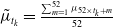 $\tilde{\mu}_{t_k} =\frac{\sum_{m=1}^{52}\mu_{52\times t_k +m}}{52}$
. The
 $98.94$
th percentile of all values
 $\{\tilde{\mu}_{t_k}\;:\; k=1,\ldots,5\}$
will be the estimated value of the attachment point
 $\hat a$
.
Given the expected loss data information, we can set up the equation
 $\mathbb{E}\left[\mathrm{PRF} (\tilde{\mu})\Big|\mathrm{PRF}(\tilde{\mu}) \gt 0 \right] \times \Pr\left(\mathrm{PRF}(\tilde{\mu}) \gt 0\right) = 0.75\%.$
The detachment point b can be estimated by solving the above equation via minimizing the function
 \begin{align*}f(b) = \left|\frac{1}{N}\sum_{i=1}^N \min\left(1, \sum_{t_k= 1}^T \frac{(\tilde{\mu}_{i, t_k} - a)_+ - (\tilde{\mu}_{i, t_k} - b)_+}{b - a} \right) - \frac{0.75\%}{1.06\%}\right|, \end{align*}
where
 $\tilde{\mu}_{i, t_k}$
is the ith simulated value of
 $\tilde{\mu}_{t_k}$
that satisfies
 $\tilde{\mu}_{i, t_k} \gt a$
, and N is the number of simulated trajectories such that the attachment point is triggered.
Our last step is to find the value of the risk premium
 $\gamma_2$
such that the coupon rate 3% satisfies the pricing Equation (24). To achieve this purpose, we implement the grid search method for the target value
 $\gamma_2$
in the interval [0, 2] with step size
 $0.001$
, such that
 \begin{align*}3\% = \frac{1 - P(0, T) + \frac{1}{N} \sum_{i=1}^N \min\left(1, \sum_{t_k= 1}^T \frac{(\tilde{\mu}_{i, t_k} - a)_+ - (\tilde{\mu}_{i, t_k} - b)_+}{b - a} \right) \times e^{- \sum_{t_k=1}^5 \sum_{m=1}^{52} r_{i, 52t_k + m}}}{\frac{1}{m}\sum_{0 \lt t_k \leq T}P(0, t_k)} \end{align*}
holds numerically, where
 $r_{i, 52t_k + m}$
are the simulated short rates under pricing measure
 $\mathbb{Q}$
. The optimal value for the risk premium
 $\gamma_2$
is finally found to be
 $\hat\gamma_2 = 1.0620$
.
6.3. Baseline analysis
After calibrating the model and pricing parameters to real mortality data and market information, we now analyze a 5-year catastrophe mortality bond structured similarly to the Vita VI bond. We set the face value to
 $F = 100$
and assume that the bond makes annual payments according to the formula (16). The mortality index that determines the bond’s principal reduction factor is defined as the yearly average mortality rate over the 5-year term. We use simulated paths of mortality and interest rates under measure
 $\mathbb{Q}$
to determine the coupon rate, and under measure
 $\mathbb{P}$
to compute the present value of the bond’s payouts at issuance (i.e., time 0).
Simulated paths of weekly mortality rates (left) and interest rates (right) with 95% confidence intervals under
 $\mathbb{Q}$
-measure.

6.3.1. Simulation of mortality and interest rates
We begin by presenting the forecast results generated by our calibrated model under the risk-neutral measure
 $\mathbb{Q}$
. These simulated paths are used to calculate the fair coupon rate c based on Equation (24). The simulated mortality rates are computed as the sum of the excess mortality rates generated by our model and the expected death rate
 $\mathbb{E}[D_t/E_t]$
. Recall from Section 6.1 that
 $\mathbb{E}[D_t/E_t]$
is estimated as the average of the weekly mortality rates observed during the years 2015–2019 (i.e., the pre-COVID years of our dataset).
Figure 3 shows the simulated weekly paths of mortality and interest rates over a 250-week period. Each plot includes three representative simulation paths, along with the estimated mean and 95% confidence intervals. The simulations are generated using our calibrated model under the pricing measure
 $\mathbb{Q}$
. The left panel shows the mortality rates fluctuating around the seasonal means with occasional upward spikes, while the right panel shows simulated interest rates that exhibit strong mean-reverting behavior within a plausible range around 3% to 9%, consistent with historical interest rate behavior. The gradual widening of the confidence intervals in both panels highlights the persistence and increasing uncertainty over time, a feature well captured by our mfBm model structure.
6.3.2. Principal repayment
We now investigate the payments of the catastrophe mortality bond using our calibrated model under the physical measure
 $\mathbb{P}$
. Specifically, we analyze the distribution of principal repayment and total payouts based on simulated mortality and interest rates. Figure 4(a) presents the distribution of simulated principal repayment values at time 0, computed under the physical measure
 $\mathbb{P}$
. Each value represents the time-0 present value of the principal repayment paid at maturity, discounted using the corresponding simulated interest rate paths. The repayment amount is determined by the principal reduction factor, which is calculated using the simulated mortality rate paths over the bond’s 5-year term.
Risk measures for the present value (PV) of principal repayment and the present value of total bond payouts under the physical measure
 $\mathbb{P}$
.

Table 3. Long description
A table comparing risk measures for the present value of principal repayment and total bond payouts under the physical measure. The table has two rows and seven columns. The columns are labeled Mean, Std, VaR 5 percent, CTE 5 percent, VaR 1 percent, and CTE 1 percent. The first row represents the present value of principal repayment with values: Mean 80.34, Std 7.91, VaR 5 percent 73.43, CTE 5 percent 61.48, VaR 1 percent 67.52, and CTE 1 percent 19.93. The second row represents the present value of total bond payouts with values: Mean 105.37, Std 8.30, VaR 5 percent 97.36, CTE 5 percent 85.40, VaR 1 percent 90.74, and CTE 1 percent 44.76.
Histogram of simulated present values of principal repayment (left) and total payouts (right) at time 0, computed under the physical measure
 $\mathbb{P}$
using simulated mortality and interest rate paths.

The main histogram of Figure 4(a) shows the distribution of discounted principal repayments across all simulated mortality and interest rate scenarios. A large proportion of the mass is concentrated near full repayment, reflecting typical cases where the mortality index remains below the attachment point and investors recover the entire principal. To better examine tail risks, the figure includes a zoom-in on the lower repayment region, specifically values between 10 and 60. This region corresponds to extreme mortality scenarios, where high mortality rates trigger significant reductions in principal repayment. Lastly, a small but noticeable proportion of the mass is concentrated at zero repayment, indicating the likelihood of the most severe cases.
Table 3 summarizes key numerical risk measures of the simulated principal repayment values at time 0. Specifically, we report the mean, standard deviation (Std), Value-at-Risk at the 5% level (VaR
 $_{5\%}$
) and 1% level (VaR
 $_{1\%}$
), and Conditional Tail Expectation at the 5% level (CTE
 $_{5\%}$
) and 1% level (CTE
 $_{1\%}$
). The mean repayment amount is approximately
 $80.34$
, indicating that investors typically recover a substantial portion of the principal under common mortality scenarios. The tail risk measures offer a deeper insight into extreme scenarios. The VaR
 $_{5\%}$
value of
 $73.43$
indicates that there is a 5% probability that principal repayment will fall below this threshold, while the CTE measures emphasize the severity of these tail scenarios. The CTE
 $_{5\%}$
at
 $61.48$
and the substantially lower CTE
 $_{1\%}$
at
 $19.93$
clearly show that extreme mortality events can lead to substantial losses.
6.3.3. Total payouts
Next, we analyze the bond’s total payouts, including both coupon payments and principal repayments. All payouts are discounted to the present values at time 0 using the corresponding simulated interest rate paths. Principal repayments are adjusted according to the simulated mortality paths. Examining this result provides a comprehensive view into the overall financial performance of the bond under simulated scenarios.
Figure 4(b) displays the distribution of simulated bond payouts, reflecting both coupon payments and principal repayments discounted to time 0. The main histogram shows that most simulated scenarios result in total payouts above the face value (
 $F=100$
), driven by the relatively high coupon rate. The zoom-in region highlights rare but severe outcomes, corresponding to significant principal reductions triggered by extreme mortality scenarios. Lastly, a small number of simulated scenarios correspond to complete principal loss, resulting in total payouts of only about 20–30 from coupon payments alone.
Table 3 provides numerical risk measures summarizing the distribution of the bond’s total payouts at time 0. The mean payout is approximately 105.37, indicating an expected outcome slightly above par value due to the high coupon accruals. The standard deviation of 8.30 reflects noticeable variability arising from mortality and interest rate uncertainties. The VaR
 $_{5\%}$
of 97.36 and VaR
 $_{1\%}$
of 90.74 highlight potential losses in adverse mortality scenarios, while the corresponding CTE values underscore the severity of these tail events, with CTE
 $_{5\%}$
at 85.40 and CTE
 $_{1\%}$
dropping to only 44.76.
6.4. Sensitivity analysis
In this subsection, we conduct a series of sensitivity analyses to better understand how the bond’s outcomes respond to changes in input assumptions. We examine key quantities, including loss metrics, payout measures, and the fair coupon rate. Three categories of parameters are considered: (i) bond design features, such as attachment and detachment points; (ii) model parameters estimated under the physical measure; and (iii) pricing parameters calibrated under the risk-neutral pricing measure. Each scenario builds on the baseline results presented earlier. Unless otherwise specified, all other inputs and bond settings remain fixed at their baseline values.
6.4.1. Sensitivity to bond parameters
We first analyze how bond structural parameters, namely, the attachment point, detachment point, and bond duration, influence the fair coupon rate of a catastrophe mortality bond.
Figure 5 presents a heatmap of the fair coupon rate as a function of the attachment and detachment points, expressed as multiples of the mortality experience in the bond issue year 2024. As expected, the coupon rate decreases monotonically as either the attachment point or the detachment point increases. A higher attachment point reduces the likelihood of triggering principal reduction, while a higher detachment point limits the severity of potential principal losses.
More interestingly, the sensitivity shown in Figure 5 is not uniform across the parameter space. We observe that changes in the detachment point have a more pronounced effect when the attachment point is low. As the attachment point increases, the fair coupon rate becomes less sensitive to further increases in the detachment point. This pattern reflects a diminishing marginal effect of expanding the reduction coverage once the probability of triggering any principal reduction becomes sufficiently small.
Table 4 reports pricing metrics for catastrophe mortality bonds with maturity terms from 1 to 5 years, including the principal repayment’s PFL, conditional expected loss (CEL), expected loss (EL), and the fair coupon rate. All values are based on 10,000 simulations under the calibrated risk-neutral measure
 $\mathbb{Q}$
. As the bond term shortens, both the probability and severity of losses decline, reflecting reduced exposure to extreme mortality events. This further leads to lower risk premiums, as reflected in steadily decreasing coupon rates.
Loss metrics of the principal repayment and fair coupon rates for catastrophe mortality bonds with varying maturity terms, calculated under the risk-neutral measure
 $\mathbb{Q}$
.

Table 4. Long description
The table presents pricing metrics for catastrophe mortality bonds with maturity terms ranging from 1 to 5 years. It includes columns for principal repayments PFL, conditional expected loss (CEL), expected loss (EL), and the fair coupon rate. The table has five rows, each corresponding to a different maturity term: 5 years (baseline), 4 years, 3 years, 2 years, and 1 year. Row 1: 5 years (baseline), PFL 1.06 percent, CEL 70.75 percent, EL 0.75 percent, Coupon rate 5.68 percent. Row 2: 4 years, PFL 0.79 percent, CEL 70.74 percent, EL 0.56 percent, Coupon rate 5.55 percent. Row 3: 3 years, PFL 0.36 percent, CEL 68.56 percent, EL 0.25 percent, Coupon rate 5.36 percent. Row 4: 2 years, PFL 0.15 percent, CEL 58.20 percent, EL 0.08 percent, Coupon rate 5.13 percent. Row 5: 1 year, PFL 0.00 percent, CEL N/A, EL N/A, Coupon rate 4.83 percent.
Heatmap showing the fair coupon rate as a function of the attachment point and detachment point, calculated under the risk-neutral pricing measure
 $\mathbb{Q}$
.

The fair coupon drops from 5.68% for a 5-year bond to 4.83% for a 1-year bond. For the 1-year bond, no loss events were observed, so CEL and EL are not reported. The corresponding coupon rate thus reflects only interest rate risk. Although the CEL remains nearly unchanged between the 4-year and 5-year bonds, the expected loss decreases slightly, consistent with the reduction in PFL from 1.06% to 0.79%. These results showcase how bond duration affects loss likelihood, severity and coupon rate of catastrophe mortality bonds.
6.4.2. Sensitivity to model parameters
We now investigate the sensitivity of bond outcomes to various model parameters. In particular, we consider the following scenarios:
-
• Scenario 1: The instantaneous correlation parameter is set to zero.
-
• Scenario 2: The Hurst parameters for both
$r_t$
and
$\mu_t$
are set to 0.5. -
• Scenario 3: The variance parameter of the interest rate process is doubled.
-
• Scenario 4: The variance parameter of the excess mortality rate process is doubled.
-
• Scenario 5: The pricing parameter associated with
$r_t$
is increased by 50%. -
• Scenario 6: The pricing parameter associated with
$\mu_t$
is increased by 50%.


Table 5 reports the fair coupon rate of the bond under each scenario, along with summary statistics and loss metrics for the present value of total bond payouts. For reference, the corresponding quantities under the baseline scenario are also included. As in the baseline case, the fair coupon rates are determined using simulations under the risk-neutral measure
 $\mathbb{Q}$
, while the payout risk measures are computed under the physical measure
 $\mathbb{P}$
.
Sensitivity analysis results for the scenarios under consideration. Each row reports summary statistics of the present value of total bond payouts (mean, standard deviation, VaR, CTE), loss metrics of the principal repayment (PFL, CEL, EL), and the fair coupon rate.

Table 5. Long description
The table presents sensitivity analysis results for various scenarios, focusing on the present value of total bond payouts and associated metrics. It includes seven rows and nine columns. The columns are labeled as Scenario, Mean, Std, VaR, CTE, PFL (%), CEL (%), EL (%), and Coupon rate (%). The row labels include Baseline, Scenario 1, Scenario 2, Scenario 3, Scenario 4, Scenario 5, and Scenario 6. Each row provides values for the mean, standard deviation, VaR, CTE, PFL, CEL, EL, and coupon rate for each scenario. Notable trends include variations in the mean, standard deviation, and coupon rates across different scenarios, with Scenario 4 showing the highest standard deviation and Scenario 5 the highest mean. The table provides a detailed comparison of how different scenarios affect the bond payouts and associated metrics.
Scenarios 1 and 2 examine the effects of removing key dependence structures between mortality and interest rates. When correlation is removed in Scenario 1, the coupon rate increases noticeably and payout risk measures shift relative to the baseline, indicating that short-term co-movement between the two processes materially influences pricing. In contrast, removing LRD in Scenario 2 results in a small reduction in the coupon rate and noticeably lower tail risk, suggesting that long-memory effects remain important for characterizing extreme outcomes. These findings confirm the need of incorporating both correlation and long-memory features into the joint modeling framework, as each plays a distinct role in shaping risk and return in catastrophe mortality bonds.
Scenarios 3 and 4 examine the effects of higher volatility in the interest rate process and the excess mortality rate process, respectively. Doubling the variance of interest rate in Scenario 3 leads to a noticeable increase in the coupon rate and greater variability in the bond payouts, indicating that interest rate volatility has a meaningful influence on bond pricing and return uncertainty. In contrast, doubling the variance of mortality rate in Scenario 4 results in a dramatic increase in tail risk, accompanied by a significantly higher coupon rate. This result suggests that mortality volatility is a comparatively stronger driver of both pricing and risk in catastrophe mortality bonds.
Scenarios 5 and 6 assess the impact of higher risk premiums for interest rate risk and mortality risk, respectively. In Scenario 5, increasing the interest rate risk premium leads to a noticeable increase in the coupon rate, reflecting the higher compensation required by investors for bearing additional interest rate risk. In Scenario 6, increasing the mortality risk premium by the same proportion produces a more moderate increase in the coupon rate. Overall, interest rate risk premiums have a stronger influence on investor compensation than mortality risk premiums. Lastly, the loss metrics under both scenarios remain unchanged relative to the baseline because these metrics are irrelevant to how risks are compensated under the risk-neutral measure
 $\mathbb{Q}$
.
7. Conclusion
In conclusion, this paper presents a novel bivariate framework grounded in a mixed fractional Brownian motion to jointly capture the LRD and instantaneous correlation between interest rate and excess mortality rate. By deriving the closed-form pricing formula for the zero-coupon bond and the pricing method for the mortality catastrophic bond under risk-neutral measure, we provide a tractable approach for valuing MLS in the environment characterized by persistent and correlated risks.
The proposed sequential calibration method facilitates the practical estimation of the model parameters from real-world data. Our numerical experiments reveal that both interest rate and mortality risks are significant risk drivers for catastrophe mortality bonds. We demonstrate that the incorporation of long-term memory and cross-risk dependence should be considered for the design of MLS. These findings offer valuable insights for actuaries and risk managers who seek innovative ways to better design and price mortality-linked instruments and the related risk management strategies.
To facilitate practical adoption of the proposed framework, we briefly summarize the implementation workflow for practitioners. The data requirements are weekly all-cause mortality data and short-term interest rate data, as described in Section 6.1. Model calibration follows the sequential procedure described in Section 5, specifically Steps 1–6 in Section 5.2 for the model parameters and Steps 1–3 in Section 5.3 for the pricing parameters. Once calibrated, the model can be used to price mortality-linked securities, such as catastrophe mortality bonds using the analytical formulas derived in Section 4, including Theorem 4.2 and Equation (17). Sensitivity analysis can then be performed by varying key parameters as illustrated in Section 6.4.
We acknowledge that there are limitations in our current work, and there remain research problems that are worth more in-depth explorations in the near future. First, excess mortality depends on the choice of baseline mortality. The risk associated with baseline mortality has not been explicitly considered in the design of MLS. It will be interesting to evaluate the impact of the choice of baseline mortality rates on the MLS design. Alternatively, we can refine our stochastic differential equations to model the mortality rate directly by adding features such as seasonality.
Second, our work can be extended to study the mortality index and explore the design of other MLS based on mortality indexes. Lastly, while the current framework assumes a constant instantaneous correlation between mortality and interest rates, it would be valuable to explore more flexible correlation structures and develop corresponding calibration techniques, particularly in light of the empirical challenge posed by having only a single observed trajectory for each process.
Third, while the mfBm framework captures the blend of transitory and persistent effects in a parsimonious and continuous manner, it is not designed to accommodate permanent structural shifts in mortality or interest rate dynamics. Certain events, such as medical technology breakthroughs, may have permanent or quasi-permanent effects on mortality dynamics, making regime-switching models a natural alternative specification (Gao et al., Reference Gao, Mamon, Liu and Tenyakov2015). Integrating such regime-switching specifications with the mfBm framework is a promising direction for future research.
Fourth, our numerical illustration lags the two data series by three weeks to reflect the response time of monetary policy changes, but does not address this lagging relationship within the model structure itself. A more principled treatment would incorporate the lag directly into the bivariate SDE system, for example, through a system of delayed stochastic differential equations in which
 $r_t$
is driven by
 $\mu_{t-\ell}$
for some lag parameter
 $\ell$
. Such a framework would yield model-consistent results, remove the need for ad hoc data alignment, and constitutes a promising direction for future research.
Lastly, exploratory calibration of the model to only the pre-pandemic data (2015–2019) suggests that the Hurst parameters are broadly stable across sample periods, indicating that LRD is a persistent feature of both series. The excess mortality process exhibits a long-term mean close to zero, and the estimated correlation shifts from strongly negative to mildly positive once the pandemic period is excluded. A more systematic comparison across pre-pandemic, in-pandemic, and post-pandemic sample periods would further inform the calibration and pricing of mortality-linked securities.
Supplementary material
The supplementary material for this article can be found at https://doi.org/10.1017/asb.2026.10111
Funding statement
Kenneth Q. Zhou acknowledges the support of the Natural Sciences and Engineering Research Council of Canada (RGPIN-2025-04157 and DGECR-2025-00488).
Competing interests
The authors declare none.


 σ
 α=0
 m=10
 θ=1

 μ~=max0≤t≤Tμt
 H2
 105
 μt
 α=0
 σ=0.116724
 m=0.008818679
 θ=1.029601
 μ0=−0.085646188



 Q

 P
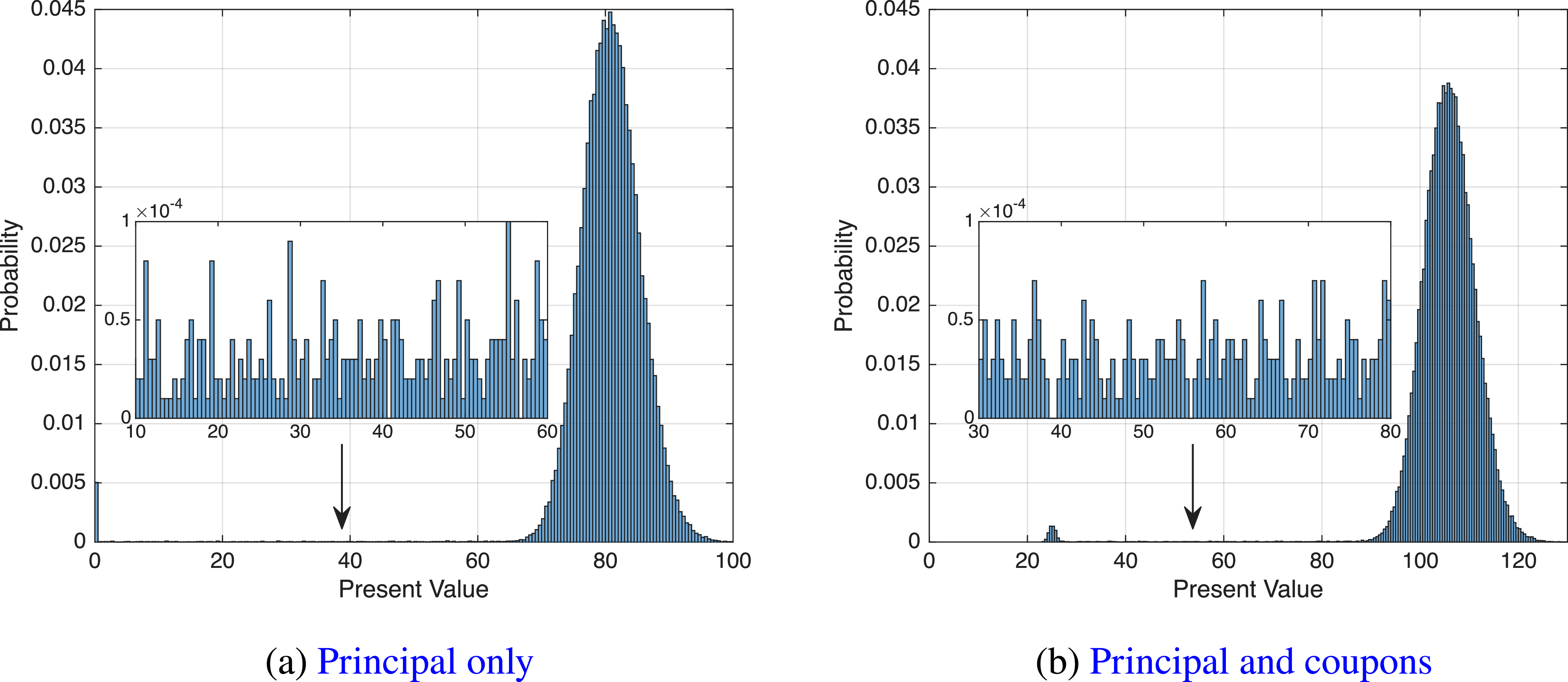
 P
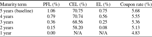
 Q
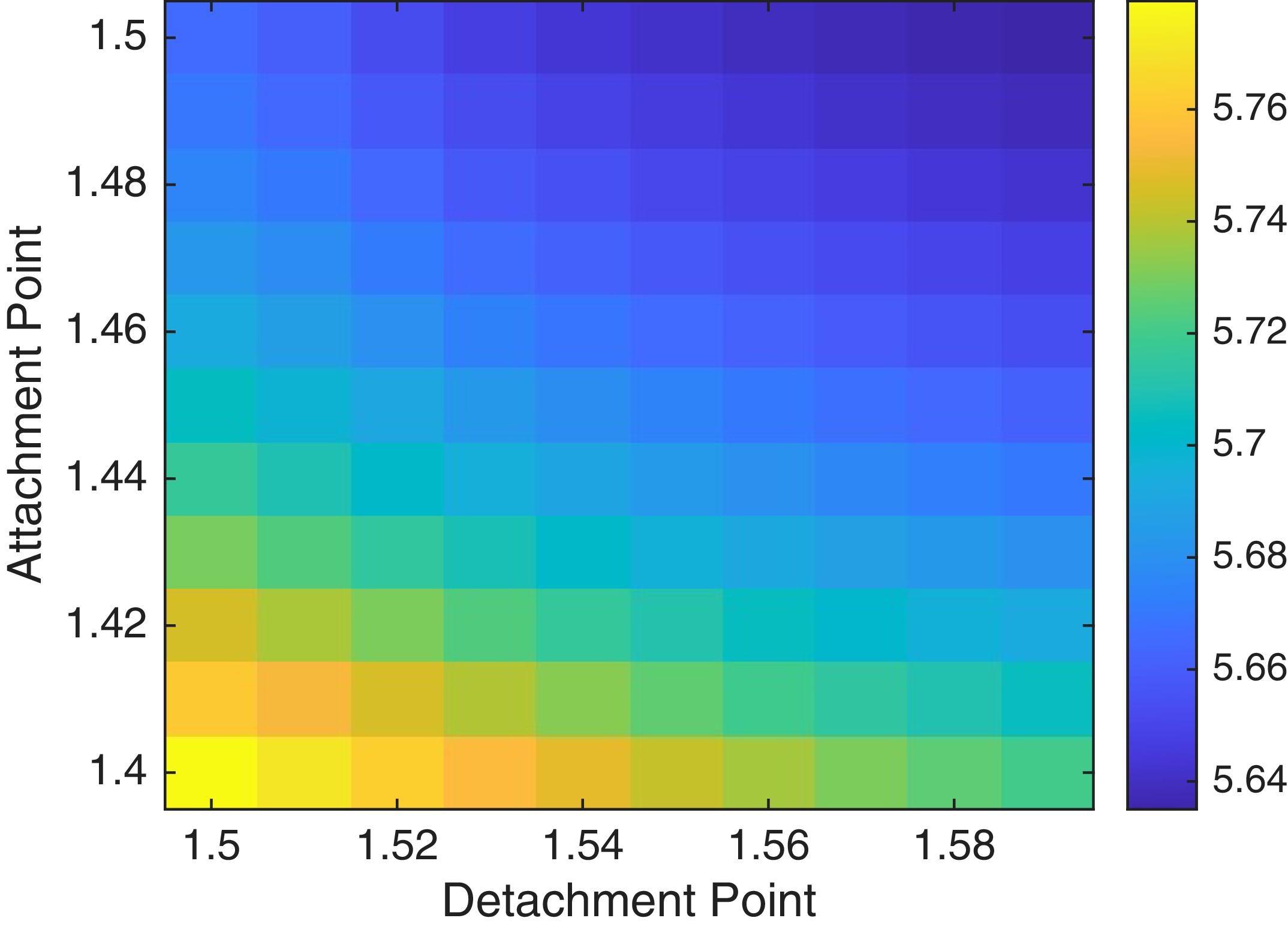
 Q
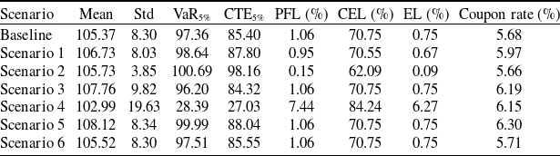


 Open access

