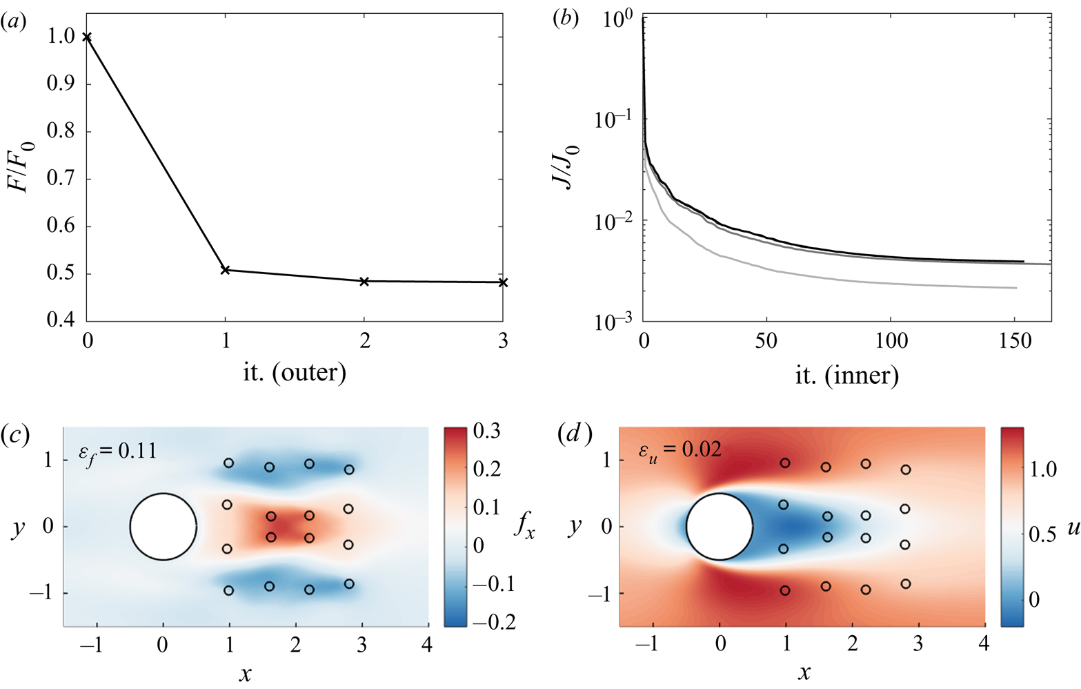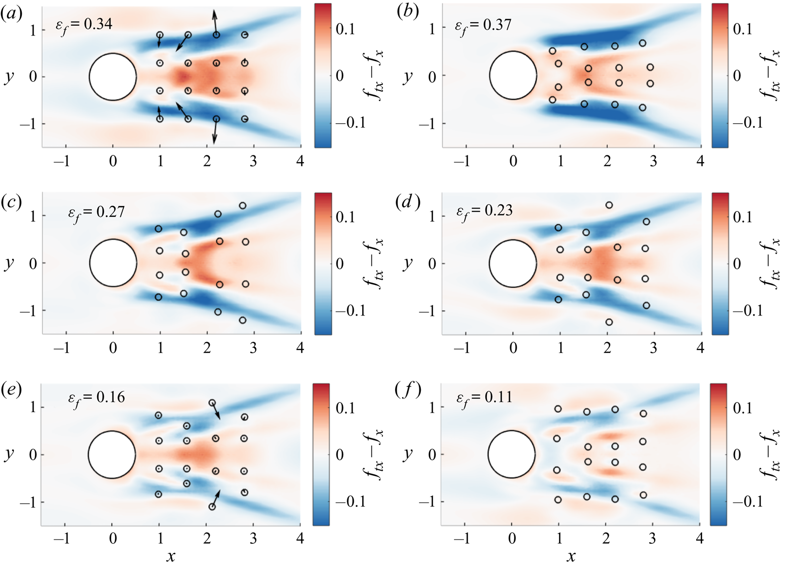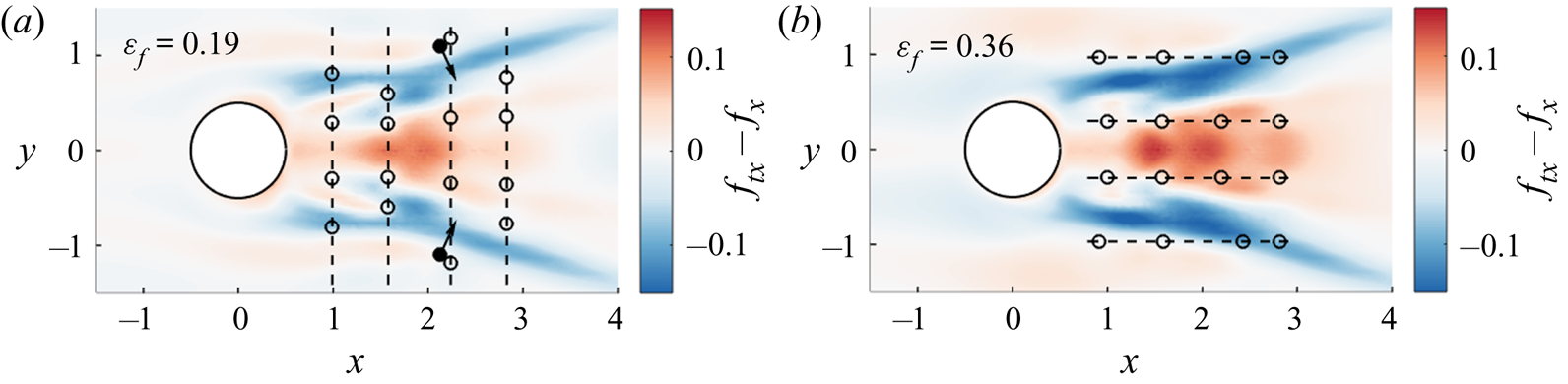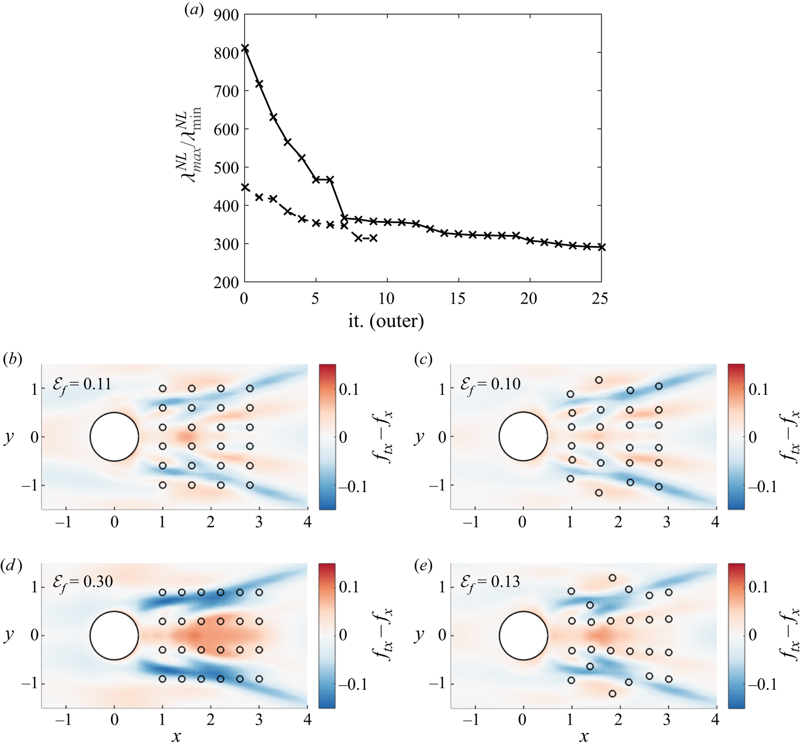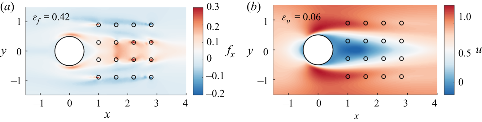


1. Introduction
Reynolds-averaged Navier–Stokes (RANS)-based simulations remain essential for the prediction of complex turbulent flows, despite their well-known limitations which originate from the need to model all turbulent scales in this framework. In parallel with the continuation of more classical approaches to address the closure problem in the RANS equations (Durbin Reference Durbin2018), the latter problem is currently revisited through the consideration of alternative strategies which may be interlinked, as will be detailed in the following: uncertainty quantification (Xiao & Cinnella Reference Xiao and Cinnella2019), data assimilation (Lewis, Lakshmivarahan & Dhall Reference Lewis, Lakshmivarahan and Dhall2006) and data-driven modelling (Duraisamy, Iaccarino & Xiao Reference Duraisamy, Iaccarino and Xiao2019). In particular, data assimilation aims to merge experimental and numerical approaches in order to overcome their inherent limitations, namely the difficulty in accessing the whole state of the flow in experiments (Heitz, Mémin & Schnörr Reference Heitz, Mémin and Schnörr2010; Suzuki Reference Suzuki2012; Gillissen, Bouffanais & Yue Reference Gillissen, Bouffanais and Yue2019) and the lack of knowledge of the inputs and models in numerical simulations (Hayase Reference Hayase2015; Meldi & Poux Reference Meldi and Poux2017; Chandramouli, Mémin & Heitz Reference Chandramouli, Mémin and Heitz2020; Da Silva & Colonius Reference Da Silva and Colonius2020; Li et al. Reference Li, Zhang, Dong and Abdullah2020).
Such a data assimilation approach was proposed by Foures et al. (Reference Foures, Dovetta, Sipp and Schmid2014) in the context of RANS, where the term that corresponds to the divergence of the Reynolds stress tensor in the momentum equations for the mean flow is considered as an adjustable forcing. The latter is optimized in order to match mean-flow measurements relying on a variational, i.e. adjoint-based, data assimilation technique (Le Dimet & Talagrand Reference Le Dimet and Talagrand1986). This methodology was notably used in conjunction with particle image velocimetry (PIV) data (Symon et al. Reference Symon, Dovetta, McKeon, Sipp and Schmid2017), and extended based on resolvent analysis for unsteady flow reconstruction (Beneddine et al. Reference Beneddine, Yegavian, Sipp and Leclaire2017; He et al. Reference He, Liu, Gan and Lesshafft2019; Symon, Sipp & McKeon Reference Symon, Sipp and McKeon2019). In parallel, the so-called field inversion approach was introduced by Singh & Duraisamy (Reference Singh and Duraisamy2016). The latter still relies on variational data assimilation, but the variables with respect to which optimization is performed, which may be referred to as the control vector, correspond to a multiplicative correction to the production term in the governing equation for the turbulent viscosity in the framework of the Boussinesq approximation. In this study, an application of data assimilation to uncertainty quantification was also illustrated, as data assimilation may provide statistics of quantities of interest in the RANS predictions that are conditioned by the available data (Wikle & Berliner Reference Wikle and Berliner2007; Xiao & Cinnella Reference Xiao and Cinnella2019). Going one step further, Parish & Duraisamy (Reference Parish and Duraisamy2016), Holland, Baeder & Duraisamy (Reference Holland, Baeder and Duraisamy2019) proposed generalizing the model corrections obtained through data assimilation with machine learning techniques, thereby resulting in data-driven predictive RANS models. It may be worth noting that non-intrusive methodologies based on ensemble Kalman filtering were also applied to the identification of turbulence model corrections (Kato et al. Reference Kato, Yoshizawa, Ueno and Obayashi2015; Xiao et al. Reference Xiao, Wu, Wang, Sun and Roy2016). However, adjoint-based techniques will still be employed in the present study due to their efficiency in evaluating both first- and second-order sensitivities, as discussed in the following. Data assimilation therefore appears as a prominent tool in all above mentioned data-driven approaches in the context of RANS modelling. The question of the appropriate choice of the model correction which forms the control vector in the data assimilation procedure remains open, and is discussed in Xiao & Cinnella (Reference Xiao and Cinnella2019), Franceschini, Sipp & Marquet (Reference Franceschini, Sipp and Marquet2020).
Whether data assimilation is employed to identify model corrections or especially to extrapolate experimental measurements, it may rely on incomplete data, i.e. the data do not correspond to the full mean flow. Instead, we consider in the present study the case where mean velocity data are only available at a few locations in the flow, which could have been obtained, for example, through laser-Doppler or hot-wire anemometry in an experimental setting. In such a situation, one may wonder how to determine appropriate measurement locations in order to enhance the fidelity of the reconstructed flow with respect to the true one. While this so-called sensor placement problem may be addressed in the context of other flow reconstruction techniques that are based, for example, on the proper orthogonal decomposition (Mokhasi & Rempfer Reference Mokhasi and Rempfer2004; Cohen, Siegel & McLaughlin Reference Cohen, Siegel and McLaughlin2006; Willcox Reference Willcox2006; Yildirim, Chryssostomidis & Karniadakis Reference Yildirim, Chryssostomidis and Karniadakis2009) or sparsity promoting techniques (Manohar et al. Reference Manohar, Brunton, Kutz and Brunton2018), or in connection with flow control (Chen & Rowley Reference Chen and Rowley2011; Belson et al. Reference Belson, Semeraro, Rowley and Henningson2013; Juillet, Schmid & Huerre Reference Juillet, Schmid and Huerre2013; Akhtar et al. Reference Akhtar, Borggaard, Burns, Imtiaz and Zietsman2015; Oehler & Illingworth Reference Oehler and Illingworth2018), it will be here investigated in the framework of variational data assimilation for RANS.
More specifically, the present study is based on the above mentioned approach of Foures et al. (Reference Foures, Dovetta, Sipp and Schmid2014) where a forcing term in the momentum equations is adjusted through data assimilation. The aim of the proposed sensor placement strategies will therefore be to improve the performance of this flow reconstruction procedure. In the following, the distinction between two objectives for sensor placement will be emphasized. On the one hand, we will aim to improve the extrapolation capacities of data assimilation, i.e. the reconstruction of the full mean velocity field from a few punctual measurements. On the other hand, the enhancement of the inversion abilities of data assimilation will be targeted, i.e. the correct identification of the forcing term from the measurements. These two objectives are clearly related, as achieving an asymptotic low error on the forcing should also lead to an improvement in the estimation of the mean velocity field. Nevertheless, they may still be treated separately in order to take into account their respective requirements, in particular in terms of number of sensors, as will be illustrated in the following.
The elaboration of methodologies to directly enhance the reconstruction of the mean velocity field will be first investigated. In the context of unsteady flows past a rotationally oscillating cylinder, Mons, Chassaing & Sagaut (Reference Mons, Chassaing and Sagaut2017) proposed a first-order adjoint-based procedure to maximize the sensitivity of the observations with respect to changes in initial and boundary conditions. In the present study, we rely on a possibly more comprehensive framework, namely the analysis of the singular vectors of the linearized model equations (Palmer et al. Reference Palmer, Gelaro, Barkmeijer and Buizza1998; Buizza & Montani Reference Buizza and Montani1999). The approach in Mons et al. (Reference Mons, Chassaing and Sagaut2017) may thus be reinterpreted as looking for capturing such dominant singular vectors, but without distinguishing between them (Rabier et al. Reference Rabier, Klinker, Courtier and Hollingsworth1996). Appropriate sensor locations for mean velocity field reconstruction will be here identified as follows. After evaluating the singular vectors of the linearized RANS equations around a given mean flow, the sensor placement will be optimized in order to enable the reconstruction of the dominant modes, as the latter may be interpreted as the most efficient in adjusting the whole mean velocity field. This approach may be considered as based on a steady resolvent analysis, as well established for the characterization of turbulent flows (Beneddine et al. Reference Beneddine, Sipp, Arnault, Dandois and Lesshafft2016; McKeon Reference McKeon2017). In addition to providing optimized sensor locations for mean velocity field reconstruction, the developed methodology may also provide an estimation of the required number of sensors to achieve a given degree of reconstruction accuracy through the analysis of a resolvent gain.
In order to improve the well posedness of the data assimilation problem and the identification of the forcing, we will build on adjoint-based sensor placement methodologies as proposed in the atmospheric sciences community, mainly in the context of unsteady problems. A large proportion of these approaches rely on the prescription of a verification cost function that measures the discrepancies in some features between the reconstructed state and a so-called verification state, which should ideally be as close as possible to the true one. Sensors may then be placed through the minimization of this verification cost function, or by directly considering its gradient. This gradient may be evaluated through a usual first-order adjoint approach (Baker & Daley Reference Baker and Daley2000; Daescu & Navon Reference Daescu and Navon2004; Langland & Baker Reference Langland and Baker2004), or by also relying on a second-order adjoint model (Daescu Reference Daescu2008; Godinez & Daescu Reference Godinez and Daescu2011; Hossen, Navon & Daescu Reference Hossen, Navon and Daescu2012; Cioaca & Sandu Reference Cioaca and Sandu2014). The second-order adjoint technique (Wang et al. Reference Wang, Navon, Le Dimet and Zou1992; Le Dimet, Navon & Daescu Reference Le Dimet, Navon and Daescu2002) allows us to rigorously take into account all nonlinearities in the data assimilation procedure and to solve meta-optimization problems that are constrained by the latter. This relatively unique ability of the variational formalism of data assimilation has favoured the consideration of the latter over stochastic and ensemble-based data assimilation techniques in the present study. While the computational developments and costs that are associated with the application of the second-order adjoint approach may appear prohibitive for unsteady systems, it should still be affordable for steady problems (Peter & Dwight Reference Peter and Dwight2010), as will be confirmed in the following. Despite their effectiveness, the above mentioned approaches for sensor placement may be limited by the need of the prescription of the verification state, which is supposed to be unknown in a pragmatic setting. Such an approach will still be considered in the present study to assess the performances of other sensor placement criteria.
Another type of technique for sensor placement is based on the spectrum of the Hessian operator, or of an approximation, that is associated with the cost function in the data assimilation problem which measures the discrepancies between the available measurements and the estimation of the flow. Sensor placement may then be formulated as the maximization of the smallest eigenvalue of this Hessian operator, or as the minimization of its condition number, in order to make all possible variations in the control vector of the data assimilation problem (here, a forcing in the momentum equations) identifiable from the measurements (Gejadze & Shutyaev Reference Gejadze and Shutyaev2012; Kang & Xu Reference Kang and Xu2012; Mons, Wang & Zaki Reference Mons, Wang and Zaki2019; Yoshimura et al. Reference Yoshimura, Yakeno, Misaka and Obayashi2020). Such approaches, which do not require knowledge about the true state beyond the available measurements, therefore enhance the well posedness of data assimilation as an inverse problem (Alekseev & Navon Reference Alekseev and Navon2001), as is well established for linear problems (Ranieri, Chebira & Vetterli Reference Ranieri, Chebira and Vetterli2014). These methodologies may also be derived in the stochastic formulation of data assimilation. The above mentioned Hessian may indeed be related to the covariance matrix that is associated with the control vector in the data assimilation problem (Le Dimet et al. Reference Le Dimet, Navon and Daescu2002; Gejadze, Shutyaev & Le Dimet Reference Gejadze, Shutyaev and Le Dimet2018). Minimizing the condition number of the Hessian may thus amount to minimizing the uncertainties in the optimal control vector. It may be emphasized that, when addressing the sensor placement problem, the above studies generally considered a linear, or linearized, inverse problem (Kang & Xu Reference Kang and Xu2012; Mons et al. Reference Mons, Wang and Zaki2019; Yoshimura et al. Reference Yoshimura, Yakeno, Misaka and Obayashi2020). In the present study, we aim to derive such a sensor placement methodology based on Hessian analysis that takes into account all nonlinearities in the data assimilation procedure in the context of RANS. We here propose to apply second-order adjoint techniques both to evaluate the Hessian operator and to evaluate the sensitivity of its spectrum with respect to sensor locations in order to optimize the latter. Through comparisons with fully linear approaches, it will be illustrated in the following that taking into account the dependency of the Hessian spectrum with respect to modifications in the reconstructed mean flow that are induced by alterations in the sensor network appears indeed necessary to actually improve the performance of data assimilation in the present case.
The paper is organized as follows. After recalling the RANS equations and specifying the considered measurements, fully linear sensor placement approaches are discussed in § 2. These methodologies focus either on the reconstruction of the mean velocity field or on the identification of a forcing in the RANS equations. The data assimilation procedure developed by Foures et al. (Reference Foures, Dovetta, Sipp and Schmid2014) to infer the full mean flow from the measurements is also recalled in this section. These techniques are applied in § 3 to the reconstruction of the mean flow around a cylinder at  $Re=150$. Motivated by the limitations of some of the present linear sensor placement approaches, second-order adjoint-based methodologies are proposed in § 4 to take into account all nonlinearities in the present inverse problem. They are then assessed in § 5. Finally, concluding remarks are made in § 6.
2. Linear sensor placement approaches for mean-flow reconstruction
In this section, the mean-flow equations for incompressible flows are first recalled in § 2.1. Following Foures et al. (Reference Foures, Dovetta, Sipp and Schmid2014), the divergence of the Reynolds stress tensor is here considered as an unknown forcing term in the momentum equations which has to be determined through data. Punctual mean velocity measurements are considered to infer this forcing. Based on a linear framework that is detailed in § 2.2, two sensor placement approaches to adjust the locations of the velocity measurements are then discussed in §§ 2.3 and 2.4. These methodologies focus respectively on enhancing the reconstruction of the full mean velocity field or that of the forcing. The reconstruction of the mean flow from the measurements is performed through the data assimilation procedure proposed by Foures et al. (Reference Foures, Dovetta, Sipp and Schmid2014), which is recalled in § 2.5.
2.1. Mean-flow equations and measurements
We consider unsteady incompressible Newtonian flows. The total non-dimensional velocity and pressure fields  $(\boldsymbol {U}(\boldsymbol {x},t)^{\top },P(\boldsymbol {x},t))^{\top }$ can be decomposed as the sum of a time-averaged mean flow
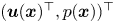 $(\boldsymbol {u}(\boldsymbol {x})^{\top },p(\boldsymbol {x}))^{\top }$ and fluctuations
 $(\boldsymbol {u}'(\boldsymbol {x},t)^{\top },p'(\boldsymbol {x},t))^{\top }$. The mean flow is thus solution of the steady RANS equations, which may be written in a compact form as
 \begin{equation} \boldsymbol{\mathcal{N}}(\boldsymbol{q})=\boldsymbol{{P}}\boldsymbol{f}, \end{equation}
where
 \begin{equation} \boldsymbol{q}=\begin{pmatrix} \boldsymbol{u} \\ p \end{pmatrix} ,\quad \boldsymbol{\mathcal{N}}(\boldsymbol{q})=\begin{pmatrix} (\boldsymbol{u}\boldsymbol{\cdot} \boldsymbol{\nabla} )\boldsymbol{u}+\boldsymbol{\nabla} p - Re^{{-}1} \varDelta \boldsymbol{u} \\ \boldsymbol{\nabla} \boldsymbol{\cdot} \boldsymbol{u} \end{pmatrix} , \quad \boldsymbol{{P}}=\begin{pmatrix} \mathbb{I} \\ 0 \end{pmatrix}. \end{equation}
The operator  $\boldsymbol {{P}}$ in (2.1) and (2.2a–c) makes the forcing term
 $\boldsymbol {f}$ act on the momentum conservation equations only. In the RANS equations, this forcing is related to the divergence of the Reynolds stress tensor according to
 \begin{equation} \boldsymbol{f}={-}\boldsymbol{\nabla} \boldsymbol{\cdot} \overline{\boldsymbol{u}'\otimes \boldsymbol{u}'}, \end{equation}
where  $\overline {\circ }$ denotes time average. While in usual RANS simulations (2.1) are closed and solved by modelling
 $\boldsymbol {f}$, e.g. by invoking the turbulent-viscosity hypothesis, we here rely on punctual mean velocity measurements and the data assimilation procedure in § 2.5 to determine
 $\boldsymbol {f}$. It should be emphasized that this forcing is here directly targeted following Foures et al. (Reference Foures, Dovetta, Sipp and Schmid2014), Symon et al. (Reference Symon, Dovetta, McKeon, Sipp and Schmid2017) and Franceschini et al. (Reference Franceschini, Sipp and Marquet2020), instead of the individual components of the Reynolds stress tensor. This may make the data assimilation problem better posed and exempt, among others, from the consideration of realizability conditions as investigated in Xiao et al. (Reference Xiao, Wu, Wang, Sun and Roy2016). It may be noticed that, if one is specifically interested in recovering the Reynolds stress tensor, the latter may still be extracted from
 $\boldsymbol {f}$ (Foures et al. Reference Foures, Dovetta, Sipp and Schmid2014).
The considered punctual measurements are performed at  $N_{{s}}$ locations and are gathered in the vector
 $\boldsymbol {y}=(\boldsymbol {y}^{(1)\top },\boldsymbol {y}^{(2)\top }, \ldots ,\boldsymbol {y}^{(N_{{s}})\top })^{\top }$ which is related to the mean flow
 $\boldsymbol {q}$ according to the compact relation
 \begin{equation} \boldsymbol{y}=\boldsymbol{h}(\boldsymbol{q}), \end{equation}
where  $\boldsymbol {h}$ is referred to as the observation operator in the following and whose application can be detailed as follows
 \begin{equation} \boldsymbol{y}^{(i)}=\int_{\varOmega}\delta(\boldsymbol{x}- \boldsymbol{x}_{{s}}^{(i)})\boldsymbol{R}\boldsymbol{q}(\boldsymbol{x})\,\textrm{d} \varOmega \quad i \in \{ 1,2,\ldots,N_{{s}}\},\quad \boldsymbol{R}=(\mathbb{I}\ 0), \end{equation}
where  $\boldsymbol {x}_{{s}}^{(i)}$ refers to the location of the
 $i$th sensor,
 $\varOmega$ is the flow domain and the restriction operator
 $\boldsymbol {R}$ extracts the velocity components from the full mean flow
 $\boldsymbol {q}$, i.e.
 $\boldsymbol {R}\boldsymbol {q}=\boldsymbol {u}$. In the next sections, we will discuss sensor placement strategies to determine appropriate sensor locations
 $(\boldsymbol {x}_{{s}}^{(i)})_{i \in \{ 1,2,\ldots ,N_{{s}}\}}$ to infer the forcing and the corresponding full mean flow from these measurements.
2.2. Linearized mean-flow equations and gain in observation space
Despite the nonlinearity of the RANS equations (2.1), we investigate in this section the possibility of deriving sensor placement criteria in a simplified, linear framework. To that end, we first consider perturbations  $\tilde {\boldsymbol {f}}$ around a reference forcing
 $\boldsymbol {f}$ which induce variations
 $\tilde {\boldsymbol {q}}$ in the corresponding mean flow
 $\boldsymbol {q}$. The question of the choice of the reference flow, which will appear to be determinant for some of the following methodologies, will be investigated in § 3.3. At first order, the perturbations
 $\tilde {\boldsymbol {f}}$ and
 $\tilde {\boldsymbol {q}}$ can be related through the resolvent operator
 $\boldsymbol {\mathcal {R}}|_{\boldsymbol {q}}$ according to
 \begin{equation} \tilde{\boldsymbol{q}}=\begin{pmatrix} \tilde{\boldsymbol{u}} \\ \tilde{p} \end{pmatrix}=\boldsymbol{\mathcal{R}}|_{\boldsymbol{q}}(\tilde{\boldsymbol{f}}), \quad \boldsymbol{\mathcal{R}}|_{\boldsymbol{q}}=\left(\left.\frac{\partial \boldsymbol{\mathcal{N}}}{\partial \boldsymbol{q}}\right|_{\boldsymbol{q}}\right)^{{-}1}\boldsymbol{{P}}, \end{equation}
which involves the tangent linear operator that is associated with the RANS equations (2.1) and is defined as
 \begin{equation} \left.\frac{\partial \boldsymbol{\mathcal{N}}}{\partial \boldsymbol{q}}\right|_{\boldsymbol{q}}(\widetilde{ \boldsymbol{q}})=\begin{pmatrix} ({\circ} \boldsymbol{\cdot} \boldsymbol{\nabla} )\boldsymbol{u}+(\boldsymbol{u}\boldsymbol{\cdot} \boldsymbol{\nabla} )\circ{-}Re^{{-}1}\varDelta \circ & \boldsymbol{\nabla} \circ \\ \boldsymbol{\nabla} \boldsymbol{\cdot} \circ & 0 \end{pmatrix} \tilde{\boldsymbol{q}}. \end{equation}
The notation  $\circ |_{\boldsymbol {q}}$ emphasizes the dependency of this operator with respect to the reference mean flow
 $\boldsymbol {q}$ around which linearization is performed. In the context of mean-flow stability analysis (Beneddine et al. Reference Beneddine, Sipp, Arnault, Dandois and Lesshafft2016; McKeon Reference McKeon2017),
 $\boldsymbol {\mathcal {R}}|_{\boldsymbol {q}}$ may be considered as the resolvent operator for zero-frequency fluctuations. The resolvent operator for fluctuations with angular frequency
 $\omega$ is indeed defined as
 $\boldsymbol {\mathcal {R}}(\omega )|_{\boldsymbol {q}}=(\mathrm {i}\omega \boldsymbol {B}+(\partial \boldsymbol {\mathcal {N}}/\partial \boldsymbol {q})|_{\boldsymbol {q}})^{-1}\boldsymbol {{P}}$, where the matrix
 $\boldsymbol {B}$ allows us to add the contribution
 $\mathrm {i}\omega$ to the first row and first column component of
 $(\partial \boldsymbol {\mathcal {N}}/\partial \boldsymbol {q})|_{\boldsymbol {q}}$ only.
As a second building block for the following methodologies, the impact of variations  $\tilde {\boldsymbol {f}}$ on the values of the measurements is then quantified through the gain
 \begin{equation} G_{\mathcal{O}}=\frac{\| \boldsymbol{h}(\tilde{\boldsymbol{q}})\|_{\mathcal{O}}^{2}}{\| \tilde{\boldsymbol{f}}\|_{\mathcal{F}}^{2}}, \end{equation}
where  $\|\circ \|_{\mathcal {O}}$ and
 $\|\circ \|_{\mathcal {F}}$ refer to the norms that are associated with the observation and forcing spaces, respectively, with
 $\|\boldsymbol {y} \|^{2}_{\mathcal {O}}=\boldsymbol {y}^{\top }\boldsymbol {y}$ and
 $\| \boldsymbol {f}\|_{\mathcal {F}}^{2}=\int _{\varOmega } \boldsymbol {f}^{\top }\boldsymbol {f}\,\textrm {d} \varOmega$. Perturbations
 $\tilde {\boldsymbol {f}}$ that are associated with small values of the gain
 $G_{\mathcal {O}}$ are hardly distinguishable from the reference forcing around which linearization is performed, while forcing variations with high gain values should be easily identifiable from the measurements. We will denote by
 $\lambda _{{max}}^{{L}}$ and
 $\lambda _{{min}}^{{L}}$ the maximum and minimum values of the gain
 $G_{\mathcal {O}}$, respectively, which appear to correspond to the maximum and minimum eigenvalues of the operator
 \begin{equation} \boldsymbol{\boldsymbol{\mathcal {H}}}^{{L}}_{\mathcal{O}}|_{\boldsymbol{q}}= \boldsymbol{\mathcal{R}}|_{\boldsymbol{q}}^{{{\dagger}}} \boldsymbol{h}^{{{\dagger}}}\boldsymbol{h}\boldsymbol{\mathcal{R}}|_{\boldsymbol{q}}. \end{equation}
The operator  $\boldsymbol{\mathcal {H}}^{{L}}_{\mathcal {O}}|_{\boldsymbol {q}}$ is self-adjoint. It involves the adjoint of the observation operator
 $\boldsymbol {h}$ in (2.4), that is defined by
 \begin{equation} \boldsymbol{h}^{{{\dagger}}}(\boldsymbol{y})= \boldsymbol{{P}} \left( \sum_{i=1}^{N_{{s}}} \boldsymbol{y}^{(i)}\delta (\boldsymbol{x}-\boldsymbol{x}^{(i)}_{{s}})\right), \end{equation}
as well as the adjoint  $\boldsymbol {\mathcal {R}}|_{\boldsymbol {q}}^{{\dagger} }$ of the resolvent operator. It is expressed as
 \begin{equation} \boldsymbol{\mathcal{R}}|_{\boldsymbol{q}}^{{{\dagger}}}=\boldsymbol{R} \left(\left(\left.\frac{\partial \boldsymbol{\mathcal{N}}}{\partial \boldsymbol{q}}\right|_{\boldsymbol{q}}\right)^{{{\dagger}}}\right)^{{-}1}. \end{equation}
This operator involves the adjoint of the tangent linear model for the RANS equations, which is defined according to
 \begin{equation} \left(\left.\frac{\partial \boldsymbol{\mathcal{N}}}{\partial \boldsymbol{q}}\right|_{\boldsymbol{q}}\right)^{{{\dagger}}}(\boldsymbol{q}^{{{\dagger}}})=\begin{pmatrix} \circ \boldsymbol{\cdot} (\boldsymbol{\nabla} \boldsymbol{u})^{\top}-(\boldsymbol{u}\boldsymbol{\cdot} \boldsymbol{\nabla} )\circ{-} Re^{{-}1} \varDelta \circ & -\boldsymbol{\nabla} \circ \\ -\boldsymbol{\nabla} \boldsymbol{\cdot} \circ & 0 \end{pmatrix} \boldsymbol{q}^{{{\dagger}}}. \end{equation}
The application of the adjoint observation operator  $\boldsymbol {h}^{{\dagger} }$ according to (2.9) thus generates a forcing to the adjoint RANS equations (2.12) that acts at the sensor locations only. The superscript
 ${L}$ in the above expressions, as in the following ones, is used to emphasize the fact that the operator
 $\boldsymbol{\mathcal {H}}^{{L}}_{\mathcal {O}}|_{\boldsymbol {q}}$ and associated eigenvalues are derived from a linear analysis, in contrast to the methodologies which will be presented in § 4.
The extremum values  $\lambda _{{max}}^{{L}}$ and
 $\lambda _{{min}}^{{L}}$ of the gain
 $G_{\mathcal {O}}$, as any eigenvalue
 $\lambda ^{{L}}_{i}$ of
 $\boldsymbol{\mathcal {H}}^{{L}}_{\mathcal {O}}|_{\boldsymbol {q}}$, verify
 \begin{equation} \boldsymbol{\mathcal {H}}^{{L}}_{\mathcal{O}}|_{\boldsymbol{q}}(\tilde{\boldsymbol{f}}_{\mathcal{O}}^{(i)})=\lambda^{{L}}_{i} \tilde{\boldsymbol{f}}_{\mathcal{O}}^{(i)},\quad \tilde{\boldsymbol{q}}_{\mathcal{O}}^{(i)}= \boldsymbol{\mathcal{R}}|_{\boldsymbol{q}}(\tilde{\boldsymbol{f}}_{\mathcal{O}}^{(i)}),\quad \tilde{\boldsymbol{u}}_{\mathcal{O}}^{(i)}= \boldsymbol{R}\tilde{\boldsymbol{q}}_{\mathcal{O}}^{(i)}, \end{equation}
where  $\tilde {\boldsymbol {f}}_{\mathcal {O}}^{(i)}$ is the eigenforcing that is associated with the eigenvalue
 $\lambda ^{{L}}_{i}$, where
 $\tilde {\boldsymbol {q}}_{\mathcal {O}}^{(i)}$ refers to the corresponding mean-flow perturbation whose velocity components are denoted by
 $\tilde {\boldsymbol {u}}_{\mathcal {O}}^{(i)}$. Eigenmodes are implicitly ordered by decreasing value of
 $\lambda ^{{L}}_{i}$.
In this linear framework, the reconstructed forcing lies in the subspace that is spanned by the  $N_{\mathcal {O}}$ eigenvectors
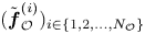 $(\tilde {\boldsymbol {f}}_{\mathcal {O}}^{(i)})_{i \in \{ 1,2,\ldots ,N_{\mathcal {O}}\}}$, where
 $N_{\mathcal {O}}$ refers to the rank of
 $\boldsymbol{\mathcal {H}}^{{L}}_{\mathcal {O}}|_{\boldsymbol {q}}$. The latter is
 $N_{\mathcal {O}}=2N_{{s}}$, i.e. twice the number of sensors, as the two velocity components of the considered two-dimensional mean flow will be measured at each sensor location.
2.3. Linear sensor placement for mean velocity field reconstruction
While the forcing  $\boldsymbol {f}$ in (2.3) forms the unknown which has to be determined through data assimilation, one could only be interested in the correct estimation of the full mean velocity field from the few punctual measurements. Directly expressing the sensor placement problem in terms of mean velocity reconstruction may be justified by the fact that improving the identification of the forcing does not necessarily imply enhancing the estimation of the full mean velocity field. This should, however, be asymptotically always true with increasing number of sensors. A second motivation, which will be illustrated in § 3.2, is that it may be easier to extrapolate the mean velocity field than correctly inferring the forcing, in the sense that less information, i.e. less sensors, is needed in the former case than in the latter one.
Relying on the linear approximation and resolvent operator  $\boldsymbol {\mathcal {R}}|_{\boldsymbol {q}}$ in (2.6a,b), we start the derivation of a sensor placement criterion for enhancing the reconstruction of the mean velocity field by quantifying global variations in the latter through the following new gain
 \begin{equation} G_{\mathcal{U}}=\frac{\| \tilde{\boldsymbol{u}}\|_{\mathcal{U}}^{2}}{\| \tilde{\boldsymbol{f}}\|_{\mathcal{F}}^{2}}, \quad \|\tilde{\boldsymbol{u}}\|_{\mathcal{U}}^{2}= \int_{\varOmega_{\mathcal{U}}}\tilde{\boldsymbol{u}}^{{T}} \tilde{\boldsymbol{u}}\,\textrm{d} \varOmega_{\mathcal{U}}, \end{equation}
where the variations in the mean velocity  $\tilde {\boldsymbol {u}}$ are evaluated in a subdomain of interest
 $\varOmega _{\mathcal {U}} \subset \varOmega$, which will be specified in the following. Similarly as in § 2.2, the gain
 $G_{\mathcal {U}}$ may be associated with the following operator
 $\boldsymbol{\mathcal {H}}^{{L}}_{\mathcal {U}}|_{\boldsymbol {q}}$ and its eigenmodes
 \begin{equation} \boldsymbol{\mathcal {H}}^{{L}}_{\mathcal{U}}|_{\boldsymbol{q}}(\tilde{\boldsymbol{f}}_{\mathcal{U}}^{(i)})=\gamma^{{L}}_{i} \tilde{\boldsymbol{f}}_{\mathcal{U}}^{(i)}\quad i \in \{ 1,2,\ldots,N_{\mathcal{U}}\},\quad \boldsymbol{\mathcal {H}}^{{L}}_{\mathcal{U}}|_{\boldsymbol{q}}= \boldsymbol{\mathcal{R}}|_{\boldsymbol{q}}^{{{\dagger}}}\boldsymbol{R}^{{{\dagger}}} \boldsymbol{R}\boldsymbol{\mathcal{R}}|_{\boldsymbol{q}}, \end{equation}
where  $N_{\mathcal {U}}$ is the number of considered eigenforcings
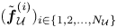 $(\tilde {\boldsymbol {f}}_{\mathcal {U}}^{(i)})_{i \in \{ 1,2,\ldots ,N_{\mathcal {U}}\}}$ with corresponding eigenvalues
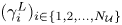 $(\gamma ^{{L}}_{i})_{i \in \{ 1,2,\ldots ,N_{\mathcal {U}}\}}$, and the adjoint
 $\boldsymbol {R}^{{\dagger} }$ of the restriction operator in (2.5) is defined with respect to the scalar product used for the mean velocity space
 $\mathcal {U}$ in (2.14). As the operator
 $\boldsymbol{\mathcal {H}}^{{L}}_{\mathcal {U}}|_{\boldsymbol {q}}$ may be of full rank, the
 $N_{\mathcal {U}}$ eigenforcings here refer only to a subset of all modes of
 $\boldsymbol{\mathcal {H}}^{{L}}_{\mathcal {U}}|_{\boldsymbol {q}}$. Furthermore, only the leading eigenmodes are relevant in the following analysis.
The most dominant eigenforcings  $(\tilde {\boldsymbol {f}}_{\mathcal {U}}^{(i)})_{i \in \{ 1,2,\ldots ,N_{\mathcal {U}}\}}$, which are associated with the largest values of the gain
 $G_{\mathcal {U}}$, may be interpreted as the most effective forcing variations in adjusting the whole mean velocity field in the domain of interest
 $\varOmega _{\mathcal {U}}$. Accordingly, it may be desirable that the forcing which is inferred from the measurements has a significant projection onto these eigenmodes, making it able to globally correct the estimation of the mean velocity field. In the present linear framework, as mentioned in § 2.2, the reconstructed forcing lies in the subspace spanned by the eigenforcings
 $(\tilde {\boldsymbol {f}}_{\mathcal {O}}^{(i)})_{i \in \{ 1,2,\ldots ,N_{\mathcal {O}}\}}$ in (2.13a–c). A sensor placement strategy may therefore consist in adjusting the sensor locations, and so the modes
 $(\tilde {\boldsymbol {f}}_{\mathcal {O}}^{(i)})_{i \in \{ 1,2,\ldots ,N_{\mathcal {O}}\}}$, so that the latter allow the best representation of the considered leading eigenforcings
 $(\tilde {\boldsymbol {f}}_{\mathcal {U}}^{(i)})_{i \in \{ 1,2,\ldots ,N_{\mathcal {U}}\}}$. This may be formulated as the minimization of the following total residual
 \begin{align} min_{(\boldsymbol{x}_{{s}}^{(k)})_{k \in \{ 1,2,\ldots,N_{{s}}\}}} \left\{ E_{\mathcal{U}}=\frac{1}{C}\sum^{N_{\mathcal{U}}}_{i=1}\gamma^{{L}}_{i} E_i\right\}, \quad E_i= \left\| \tilde{\boldsymbol{f}}_{\mathcal{U}}^{(i)} - \sum_{j=1}^{N_{\mathcal{O}}}\left\langle \tilde{\boldsymbol{f}}_{\mathcal{U}}^{(i)},\tilde{\boldsymbol{f}}_{\mathcal{O}}^{(j)} \right\rangle_{\mathcal{F}}\tilde{\boldsymbol{f}}_{\mathcal{O}}^{(j)} \right\|_{\mathcal{F}}^{2}, \end{align}
where  $E_i$ is the residual for the
 $i$th mode
 $\tilde {\boldsymbol {f}}_{\mathcal {U}}^{(i)}$ in the basis formed by
 $(\tilde {\boldsymbol {f}}_{\mathcal {O}}^{(j)})_{j \in \{ 1,2,\ldots ,N_{\mathcal {O}}\}}$ and is weighted by the corresponding eigenvalue
 $\gamma ^{{L}}_{i}$ in order to promote the most dominant modes, with
 $C=\sum ^{N_{\mathcal {U}}}_{i=1}\gamma ^{{L}}_{i}$.
The minimization in (2.16a,b) is performed with an iterative gradient-based descent method, more specifically the Polak–Ribière variant of the nonlinear conjugate gradient method. It is supplemented by the backtracking-Armijo line search algorithm (Armijo Reference Armijo1966) to identify the step size that weights the descent direction. Such an optimization technique thus requires the gradient of the total residual  $E_{\mathcal {U}}$ with respect to the sensor locations. The latter is obtained from the linear combination of the gradients for each residual
 $E_i$ according to (2.16a,b). The gradient of the residual
 $E_i$ with respect to the
 $k$th sensor location is given by
 \begin{equation} \frac{\partial E_i}{\partial \boldsymbol{x}_{{s}}^{(k)}}=2 \sum_{j=1}^{N_{\mathcal{O}}} \boldsymbol{\nabla} ( \tilde{\boldsymbol{u}}^{(j)\top}_{\mathcal{O}} \tilde{\boldsymbol{v}}^{(ij)} )(\boldsymbol{x}_{{s}}^{(k)}). \end{equation}
The above sensitivity thus corresponds to the spatial gradient, which is evaluated at the sensor locations, of the scalar product between the velocity field  $\tilde {\boldsymbol {u}}^{(j)}_{\mathcal {O}}$ in (2.13a–c) and
 $\tilde {\boldsymbol {v}}^{(ij)}=\boldsymbol {R}\tilde {\boldsymbol {s}}^{(ij)}$. This pseudo-velocity field is computed from
 $\tilde {\boldsymbol {s}}^{(ij)}=\boldsymbol {\mathcal {R}}|_{\boldsymbol {q}}(\tilde {\boldsymbol {g}}^{(ij)})$, where the pseudo-forcing
 $\tilde {\boldsymbol {g}}^{(ij)}$ is obtained from the inversion of
 \begin{equation} (\boldsymbol{\mathcal {H}}^{{L}}_{\mathcal{O}}|_{\boldsymbol{q}}- \lambda_{j}^{{L}}\mathbb{I})(\tilde{\boldsymbol{g}}^{(ij)})=\langle \tilde{\boldsymbol{f}}_{\mathcal{U}}^{(i)},\tilde{\boldsymbol{f}}^{(j)}_{\mathcal{O}} \rangle_{\mathcal{F}}\delta \tilde{\boldsymbol{f}}_{\mathcal{U}}^{(i)}, \quad \langle \tilde{\boldsymbol{g}}^{(ij)},\tilde{\boldsymbol{f}}^{(j)}_{\mathcal{O}} \rangle_{\mathcal{F}}=0, \end{equation}
where  $\delta \tilde {\boldsymbol {f}}_{\mathcal {U}}^{(i)}= \tilde {\boldsymbol {f}}_{\mathcal {U}}^{(i)} - \sum _{j=1}^{N_{\mathcal {O}}}\langle \tilde {\boldsymbol {f}}_{\mathcal {U}}^{(i)},\tilde {\boldsymbol {f}}_{\mathcal {O}}^{(j)} \rangle _{\mathcal {F}}\tilde {\boldsymbol {f}}_{\mathcal {O}}^{(j)}$.
Once a reference forcing and associated mean flow are chosen, starting from an initial sensor arrangement, the minimization problem (2.16a,b) mainly requires the computation of the eigendecomposition of the operator  $\boldsymbol{\mathcal {H}}^{{L}}_{\mathcal {O}}|_{\boldsymbol {q}}$ for the current sensor network, which is used both to evaluate the total residual
 $E_{\mathcal {U}}$ and to efficiently solve (2.18a,b). Once the gradients (2.17) are assembled, the latter allow us to update the sensor locations, this procedure being repeated until convergence.
2.4. Linear sensor placement for forcing identification
In order to ensure the well posedness of the present data assimilation problem, namely the correct identification of the forcing  $\boldsymbol {f}$ in (2.3) from the measurements, the sensor placement problem may rather be formulated as seeking sensor locations that allow us to differentiate between all possible forcings. In the present linear framework, this amounts to identifying sensor placements that make all forcing perturbations inducing non-negligible and similar energy perturbations in observation space as quantified through the gain
 $G_{\mathcal {O}}$ in (2.8). More specifically, optimal sensor placement may here be expressed as the minimization of the ratio between the maximum and minimum values of the gain
 $G_{\mathcal {O}}$, i.e.
 \begin{equation} min_{(\boldsymbol{x}_{{s}}^{(k)})_{k \in \{ 1,2,\ldots,N_{{s}}\}}} \frac{\lambda^{{L}}_{{max}}}{\lambda^{{L}}_{{min}}}. \end{equation}
This criterion may also be interpreted as the minimization of the condition number of the operator  $\boldsymbol{\mathcal {H}}^{{L}}_{\mathcal {O}}|_{\boldsymbol {q}}$ in (2.9). Similarly to § 2.3, the minimization in (2.19) is performed through the nonlinear conjugate gradient method, which requires the ability to evaluate the sensitivity of eigenvalues of
 $\boldsymbol{\mathcal {H}}^{{L}}_{\mathcal {O}}|_{\boldsymbol {q}}$ with respect to the sensor locations. The gradient of the eigenvalue
 $\lambda ^{{L}}_{i}$ with respect to the
 $k$th sensor location is given by
 \begin{equation} \frac{\partial \lambda^{{L}}_{i}}{\partial \boldsymbol{x}_{{s}}^{(k)}}= \boldsymbol{\nabla} (\tilde{\boldsymbol{u}}_{\mathcal{O}}^{(i)\top} \tilde{\boldsymbol{u}}_{\mathcal{O}}^{(i)})(\boldsymbol{x}_{{s}}^{(k)})= 2 ( \boldsymbol{\nabla} \tilde{\boldsymbol{u}}_{\mathcal{O}}^{(i)}(\boldsymbol{x}_{{s}}^{(k)}) )^{\top} \tilde{\boldsymbol{u}}_{\mathcal{O}}^{(i)}(\boldsymbol{x}_{{s}}^{(k)}), \end{equation}
which again involves the velocity field  $\tilde {\boldsymbol {u}}_{\mathcal {O}}^{(i)}$ that is associated with
 $\lambda ^{{L}}_{i}$ according to (2.13a–c). After (2.20) is applied to the maximum and minimum eigenvalues of
 $\boldsymbol{\mathcal {H}}^{{L}}_{\mathcal {O}}|_{\boldsymbol {q}}$, the gradient of their ratio in (2.19) with respect to the sensor locations is straightforwardly obtained.
As in § 2.3, the evaluation of the eigendecomposition of  $\boldsymbol{\mathcal {H}}^{{L}}_{\mathcal {O}}|_{\boldsymbol {q}}$ accounts for most of the computational cost that is required to solve (2.19). It may be noticed that this sensor placement criterion explicitly requires the smallest eigenvalue of
 $\boldsymbol{\mathcal {H}}^{{L}}_{\mathcal {O}}|_{\boldsymbol {q}}$. As networks that are formed by at most a few tens of sensors are considered in the following, as further discussed in § 3.2, the computation of
 $\lambda ^{{L}}_{{min}}$ remains feasible (see § 2.2). In the case of significantly larger sensor networks, one could consider replacing
 $\lambda _{{min}}^{{L}}$ in the criterion (2.19) with an approximation in a subset of eigenvalues of
 $\boldsymbol{\mathcal {H}}^{{L}}_{\mathcal {O}}|_{\boldsymbol {q}}$, which should still be representative of the modes with lower gain values.
2.5. Variational data assimilation for mean-flow reconstruction
Once the sensor network is selected, the variational data assimilation procedure proposed by Foures et al. (Reference Foures, Dovetta, Sipp and Schmid2014) is employed to actually infer the unknown true forcing  $\boldsymbol {f}_{{t}}$ from punctual mean velocity measurements of the true mean flow
 $\boldsymbol {q}_{{t}}$ under consideration. As we here consider sparse data, in addition to the minimization of the misfit between the measurements
 $\boldsymbol {y}$ and the mean-flow prediction, we also consider the penalization of the
 $H^{1}$ norm of the forcing. Accordingly, the data assimilation problem is here formulated as the following optimization problem
 \begin{equation} min_{\boldsymbol{f}}\left\{J=\frac{1}{2}\| \boldsymbol{y}-\boldsymbol{h}(\boldsymbol{q})\|_{\mathcal{O}}^{2}+\frac{\alpha}{2}(\|\,\boldsymbol{f} \|^{2}_{\mathcal{F}}+ \|\boldsymbol{\nabla} \boldsymbol{f} \|^{2}_{\mathcal{G}} )\right\},\quad \boldsymbol{\mathcal{N}}(\boldsymbol{q})=\boldsymbol{{P}}\boldsymbol{f}, \end{equation}
where the mean flow  $\boldsymbol {q}$ satisfies the RANS equations (second equality), and the positive real parameter
 $\alpha$ allows us to adjust the penalization of the
 $H^{1}$ norm of the forcing. The considered penalization term appears essential to prevent non-physical, very localized forcings due to the use of sparse measurements. On the other hand, the reconstructed mean velocity field remains here adequately smooth even without any regularization, which might be ascribed to the relatively low Reynolds number of the flow configuration which is considered in the following and described in § 3.1. The choice of an appropriate value for
 $\alpha$ along with the precise impact of regularization on the reconstructed flow are further discussed in § 3.1 and in Appendix B where comparisons between the use or not of penalization are provided.
The scalar product for the space  $\mathcal {G}$ in (2.21a,b) is defined in a very similar way as for
 $\mathcal {F}$ in (2.8), and differ from the latter only by taking into account the different number of components in
 $\boldsymbol {\nabla } \boldsymbol {f}$ compared with
 $\boldsymbol {f}$. As for the sensor placement problems in this section, the cost function
 $J$ in (2.21a,b) is minimized by relying on a gradient-based descent method, and we here prefer to employ the low-memory Broyden–Fletcher–Goldfarb–Shanno method (Nocedal Reference Nocedal1980). The step size for the descent direction is still determined through the backtracking-Armijo line search algorithm. The gradient of
 $J$ with respect to the forcing is given by
 \begin{equation} \left.\frac{\partial J}{\partial \boldsymbol{f}}\right|_{\boldsymbol{f}}=\boldsymbol{u}^{{{\dagger}}} +\alpha(\,\boldsymbol{f}-\varDelta \boldsymbol{f}), \end{equation}
where the velocity field components  $\boldsymbol {u}^{{\dagger} }=\boldsymbol {R}\boldsymbol {q}^{{\dagger} }$ of the adjoint variable
 $\boldsymbol {q}^{{\dagger} }$, which is introduced to take into account the constraint
 $\boldsymbol {\mathcal {N}}(\boldsymbol {q})=\boldsymbol {{P}}\boldsymbol {f}$, are obtained from
 \begin{equation} \boldsymbol{u}^{{{\dagger}}}=\boldsymbol{\mathcal{R}}|_{\boldsymbol{q}}^{{{\dagger}}} (\boldsymbol{h}^{{{\dagger}}}(\boldsymbol{h}(\boldsymbol{q})-\boldsymbol{y})), \end{equation}
where the various adjoint models are defined in (2.10)–(2.12). Further details about the derivation of the gradient (2.22) are provided in Appendix A. Starting from the first guess  $\boldsymbol {f}=\boldsymbol {f}_{{b}}=\boldsymbol {0}$, whose corresponding mean flow
 $\boldsymbol {q}_{{b}}$ will be referred to as the base flow, (2.1) and (2.23) are successively inverted in order to evaluate the gradient (2.22), which is used to update the estimation of the forcing term, this procedure being repeated until convergence. The outcome of this procedure will be referred to as the reconstructed, or assimilated flow, in the following, whose corresponding forcing and mean flow will be denoted as
 $\boldsymbol {f}_{{a}}$ and
 $\boldsymbol {q}_{{a}}$, respectively.
As detailed in Foures et al. (Reference Foures, Dovetta, Sipp and Schmid2014), observations of the mean velocity field alone allow us to reconstruct the solenoidal part of the true forcing  $\boldsymbol {f}_{{t}}$ only, as
 $\boldsymbol {f}_{{a}}$ can only be divergence free. Accordingly, in the following,
 $\boldsymbol {f}_{{t}}$ is implicitly replaced with its solenoidal contribution
 $\boldsymbol {f}^{{s}}_{{t}}$ according to the Helmholtz decomposition
 $\boldsymbol {f}_{{t}}=\boldsymbol {f}^{{s}}_{{t}}+\boldsymbol {\nabla } \phi$, with
 $\boldsymbol {\nabla } \boldsymbol {\cdot } \boldsymbol {f}^{{s}}_{{t}}=0$.
It might be worth noting that data assimilation is here considered from a deterministic point of view. The extension of the present methodologies to a stochastic formulation in order to take into account, among others, measurement noise may simply consist in modifying the definition of the above scalar products to include the covariance matrices that are associated with uncertainties in the measurements and to a prior estimation of the forcing (Lewis et al. Reference Lewis, Lakshmivarahan and Dhall2006; Wikle & Berliner Reference Wikle and Berliner2007).
3. Application of linear sensor placement
In this section, the data assimilation and linear sensor placement procedures of § 2 are applied to the reconstruction of the two-dimensional mean flow around an infinite circular cylinder from a limited number of punctual velocity measurements. Details about the flow configuration and numerical methods are provided in § 3.1, while applications of the sensor placement procedures to specifically enhance the reconstruction of the mean velocity field or that of the forcing are performed in §§ 3.2 and 3.3, respectively.
3.1. Flow configuration and numerical set-up
Similarly to Foures et al. (Reference Foures, Dovetta, Sipp and Schmid2014), we consider the two-dimensional mean flow around an infinite circular cylinder. The Reynolds number  $Re$ based on the diameter
 $D$ of the cylinder and the inlet velocity
 $U_{\infty }$ is chosen as
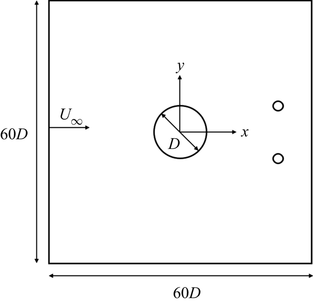
 $150$. All computations rely on the software FreeFEM++ (Hecht Reference Hecht2012) which is based on the finite element method. Taylor–Hood elements that are respectively quadratic and linear for velocity and pressure are employed. The two-dimensional computational domain is a square of side
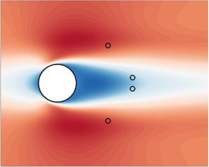
 $60D$ with the circular cylinder at its centre, as illustrated in figure 1. The considered mesh corresponds to approximately
 $7.4 \cdot 10^4$ degrees of freedom. In the above derivations, as in the following, all quantities are non-dimensionalized using
 $U_{\infty }$ and
 $D$. For the RANS model (2.1), which is solved using the Newton method,
 $\boldsymbol {u}=u\boldsymbol {e}_x+v \boldsymbol {e}_y=\boldsymbol {e}_x$ is imposed at the inlet, symmetry boundary conditions
 $({\partial u}/{\partial y},v)=(0,0)$ are used for the top and bottom boundaries, the no-slip condition
 $u=v=0$ is imposed at the cylinder, while the outflow condition
 $(Re^{-1}({\partial u}/{\partial x})-p,{\partial v}/{\partial x})=(0,0)$ is enforced at the outlet. The adjoint model in (2.12) is implemented following the discrete adjoint approach (Peter & Dwight Reference Peter and Dwight2010). The optimization procedures to solve the sensor placement and data assimilation problems (2.16a,b), (2.19) and (2.21a,b) rely on the same stopping criterion, which corresponds to a relative variation in the corresponding objective function inferior to
 $10^{-3}$ between two successive iterations.
Schematic of the flow configuration with the computational domain. The small open circles symbolize the adjustable locations of velocity sensors which will be used for mean-flow reconstruction.

Concerning specifically the data assimilation procedure, an adjustable aspect is the regularization parameter  $\alpha$ in the cost function
 $J$ in (2.21a,b) that allows us to penalize the
 $H^1$ norm of the forcing
 $\boldsymbol {f}$. Assuming that
 $U_{\infty }$ and
 $D$ are appropriate scalings for the divergence of the Reynolds stress tensor for the present flow configuration, i.e. the velocity and forcing fields are assumed to have similar magnitudes and spatial variations after non-dimensionalization, we choose the value
 $\alpha =10^{-2}$ in order to keep the observation contribution largely dominant in the cost function
 $J$ while still regularizing the data assimilation problem. It was checked that relatively large variations around the considered value (increasing or decreasing it by one order of magnitude) do not entail significant modifications in the reconstruction results. The case
 $\alpha =0$ (no regularization) is discussed in Appendix B.
In order to assess the performances of the sensor placement and data assimilation procedures, the following relative errors between the assimilated and true flows will be considered
 \begin{equation} \varepsilon_{f}=\frac{\displaystyle \int_{\varOmega_{\mathcal{U}}} \delta \boldsymbol{f}_{{a}}^{\top}\delta \boldsymbol{f}_{{a}}\,\textrm{d} \varOmega_{\mathcal{U}}}{\displaystyle \int_{\varOmega_{\mathcal{U}}} \delta \boldsymbol{f}_{{b}}^{\top}\delta \boldsymbol{f}_{{b}}\,\textrm{d} \varOmega_{\mathcal{U}}}, \quad \varepsilon_{u}=\frac{\displaystyle \int_{\varOmega_{\mathcal{U}}} \delta \boldsymbol{u}_{{a}}^{\top}\delta \boldsymbol{u}_{{a}}\,\textrm{d} \varOmega_{\mathcal{U}}}{\displaystyle \int_{\varOmega_{\mathcal{U}}} \delta \boldsymbol{u}_{{b}}^{\top}\delta \boldsymbol{u}_{{b}}\,\textrm{d} \varOmega_{\mathcal{U}}}, \end{equation}
where  $\delta \boldsymbol {f}=\boldsymbol {f}_{{t}}-\boldsymbol {f}$ is the discrepancy field between a forcing
 $\boldsymbol {f}$ and the true forcing
 $\boldsymbol {f}_{{t}}$, while
 $\delta \boldsymbol {u}=\boldsymbol {u}_{{t}}-\boldsymbol {u}$ is its counterpart for the velocity field. The control volume
 $\varOmega _{\mathcal {U}}$ in (3.1a,b) refers to the flow domain that is included in the domain
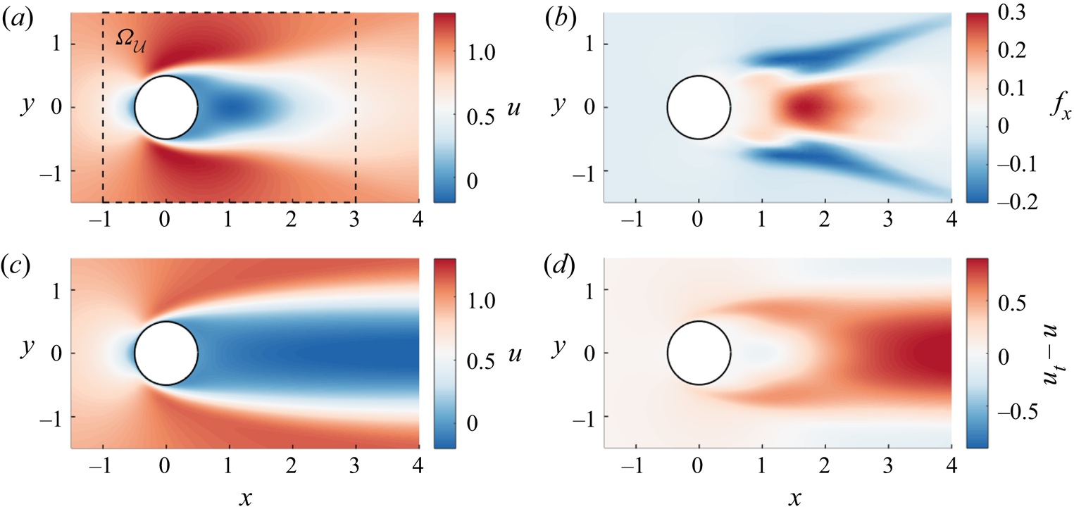
 $[-1,3 ] \times [-1.5,1.5]$ (see figure 2a), whose extent is chosen to include the whole recirculation bubble and slightly beyond in all directions, in particular upstream of the cylinder. This subdomain is the same as the one that will be chosen for the sensor placement criterion (2.16a,b). It can be noticed that, in (3.1a,b), the discrepancies between the true and assimilated flows are normalized by those between the true flow and the base flow, i.e. the first guess of the data assimilation procedure, in order to directly provide the improvement in the estimation of the mean flow through data assimilation compared with the latter.
True streamwise components of (a) the mean flow around a cylinder at  $Re=150$ and (b) corresponding forcing. (c) Streamwise velocity for the base flow and (d) associated discrepancy field. The domain of interest
 $\varOmega _{\mathcal {U}}$, which is used in both the reconstruction errors (3.1a,b) and the sensor placement criterion (2.16a,b), is reported in (a).

The considered mean-flow measurements  $\boldsymbol {y}$ for the cylinder flow at
 $Re=150$ are generated by solving the unsteady Navier–Stokes equations relying on similar numerical methods as described above. The true mean flow and associated forcing are illustrated in figure 2, along with the base flow. For the sake of compactness, in this figure as in the following ones, only the streamwise component of these fields is reported. In the following, conclusions drawn from the analysis of the streamwise component will be also valid for the cross-flow one, while it might be worth emphasizing that both components are taken into account in the quantitative error assessment (3.1a,b).
3.2. Enhancing the reconstruction of the mean velocity field
We here apply the sensor placement methodology of § 2.3 to specifically enhance the reconstruction of the mean velocity field from the few punctual measurements. The goal of the sensor placement procedure will thus be to determine sensor locations so that the inferred forcing is the most effective in correcting the estimation of the mean velocity field in the domain of interest  $\varOmega _{\mathcal {U}}$ (see figure 2a). As discussed in § 2.3, this may amount to identifying sensor locations which allow the best representation of the forcings that induce the largest perturbations in the mean velocity field according to the gain
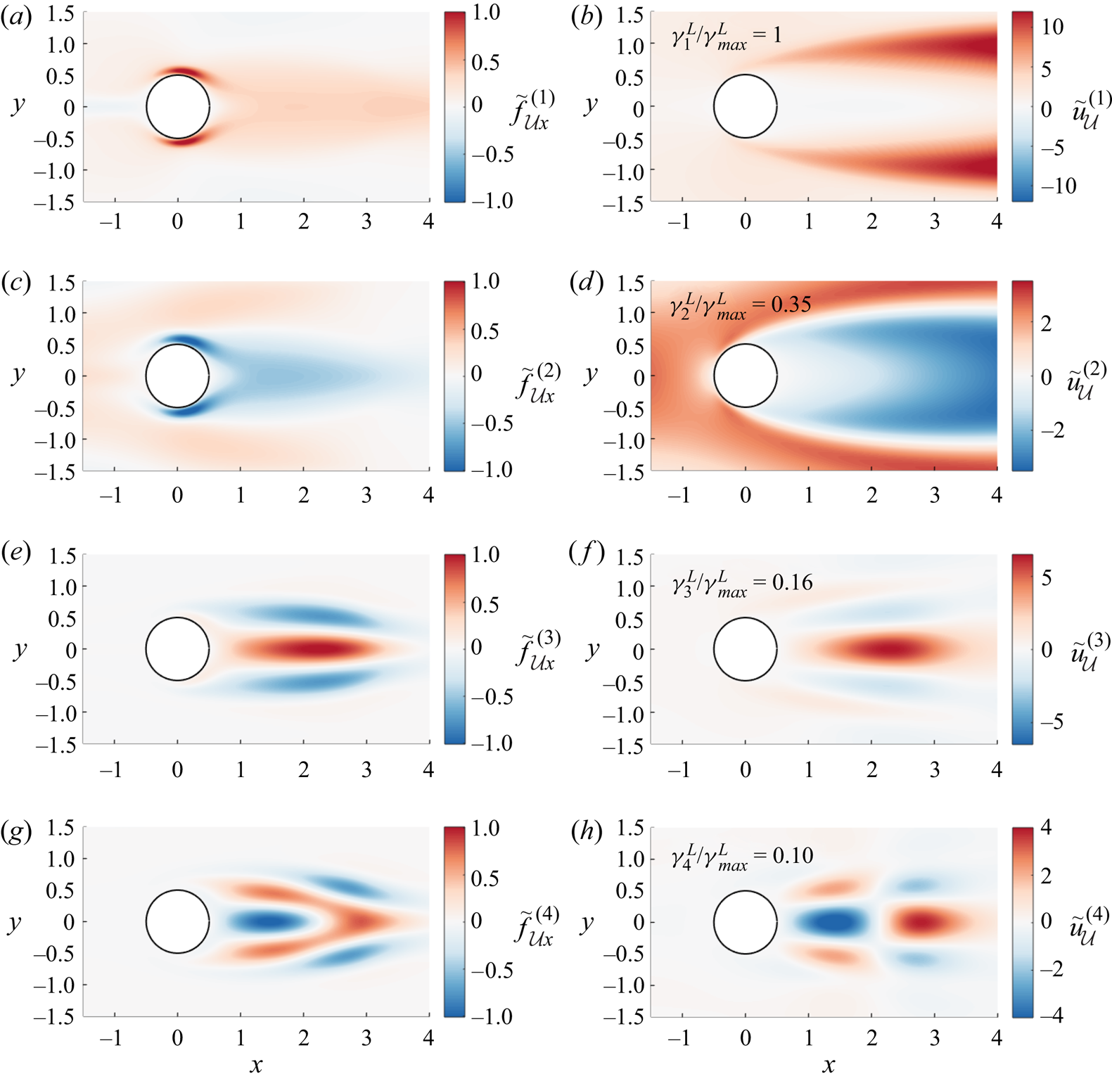
 $G_{\mathcal {U}}$ in (2.14). We chose to perform the analysis around the base flow, i.e. all linearizations in §§ 2.2 and 2.3 are made around the latter, which seems a natural choice as the base flow forms the first guess for the data assimilation procedure. Figure 3 reports the first four eigenforcings
 $\tilde {\boldsymbol {f}}_{\mathcal {U}}^{(i)}$ with the largest values of the gain
 $G_{\mathcal {U}}$. Through the minimization of the residual
 $E_{\mathcal {U}}$ in (2.16a,b), we thus aim for the best representation of these eigenforcings in the basis formed by the modes
 $(\tilde {\boldsymbol {f}}_{\mathcal {O}}^{(j)})_{j \in \{ 1,2,\ldots ,N_{\mathcal {O}}\}}$ which are associated with the gain
 $G_{\mathcal {O}}$ in observation space (2.8). From figure 3, a distinction may be made between the first two forcings
 $\tilde {\boldsymbol {f}}_{\mathcal {U}}^{(i)}$, which appear most efficient in adjusting the mean velocity outside of the wake, and the third and fourth modes, which have a strong impact on the recirculation region. The rationale behind the consideration of only these four modes is discussed below.
The first four dominant eigenmodes (from most to least dominant going from top to bottom row) which are associated with the gain  $G_{\mathcal {U}}$ in (2.14) evaluated around the base flow: streamwise component of the eigenforcing
 $\tilde {\boldsymbol {f}}_{\mathcal {U}}^{(i)}$ (left column) and associated velocity perturbation
 $\tilde {\boldsymbol {u}}_{\mathcal {U}}^{(i)}=\boldsymbol {R} \boldsymbol {\mathcal {R}}|_{\boldsymbol {q}_{{b}}}(\tilde {\boldsymbol {f}}_{\mathcal {U}}^{(i)})$ (right column). The corresponding value of the gain
 $\gamma ^{{L}}_{i}=G_{\mathcal {U}}(\tilde {\boldsymbol {f}}_{\mathcal {U}}^{(i)})$ is also reported in the figures.

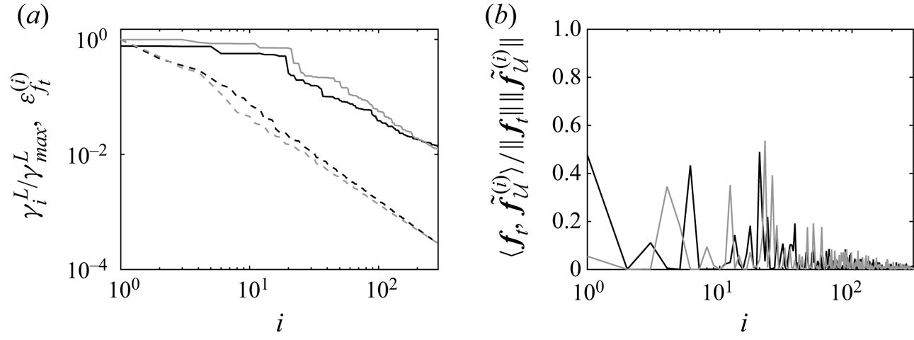
Before proceeding further, it may be instructive to further analyse the gain  $G_{\mathcal {U}}$ and relative eigenforcings in order to get insights in the respective difficulties that lie in the extrapolation problem, i.e. the possibility of getting the full mean velocity field from the measurements, which is of interest in the present section, and the inverse problem, namely the reconstruction of the forcing. Figure 4(a) reports the value of
 $G_{\mathcal {U}}$ for the modes
 $\tilde {\boldsymbol {f}}_{\mathcal {U}}^{(i)}$, along with the error that is committed on the representation of the true forcing
 $\boldsymbol {f}_{{t}}$ in the basis formed by an increasing number of these same modes. This error when relying on
 $i$ modes is defined as
 \begin{equation} \varepsilon_{f_{{t}}}^{(i)}=\frac{\int_{\varOmega_{\mathcal{U}}}\delta \boldsymbol{f}_{{t}}^{(i)\top}\delta\boldsymbol{f}_{{t}}^{(i)}\,\textrm{d} \varOmega_{\mathcal{U}}}{\int_{\varOmega_{\mathcal{U}}} \boldsymbol{f}_{{t}}^{\top}\boldsymbol{f}_{{t}}\,\textrm{d} \varOmega_{\mathcal{U}}}, \quad \delta\boldsymbol{f}_{{t}}^{(i)}=\boldsymbol{f}_{{t}}-\sum_{j=1}^{i}\langle \boldsymbol{f}_{{t}},\tilde{\boldsymbol{f}}_{\mathcal{U}}^{(j)}\rangle_{\mathcal{F}}\tilde{\boldsymbol{f}}_{\mathcal{U}}^{(j)}. \end{equation}
It appears that the value of the gain  $G_{\mathcal {U}}$ decays at a relatively high rate and that only a few modes induce significant variations in the mean velocity field. This suggests that a small number of sensors is required to correctly reconstruct the full mean velocity field in the present case. In particular, it may be noticed that the value of
 $G_{\mathcal {U}}$ for the fourth dominant mode is already one order of magnitude smaller than the maximum value. Accordingly, based on the fact that the true forcing has a non-zero projection on the most dominant modes as illustrated in figure 4(b), and assuming that a number of
 $n$ sensors allow us to reconstruct
 $n$ modes, a network of four sensors seems sufficient to already provide a correct estimation of the true velocity field, as will be confirmed in this section. On the other hand, the error
 $\varepsilon _{f_{{t}}}^{(i)}$ decays at a much lower rate, which originates from the relatively low projection of the true forcing on the dominant modes, as reported in figure 4(b). Around
 $20$ modes, and thus possibly the same number of sensors, seem necessary to decrease this error to
 $0.1$. This was used to prescribe the maximum size of the considered sensor networks in this study, namely
 $N_{{s}}=24$, such configurations being investigated in § 5.5. This discussion thus suggests that the present extrapolation problem is easier to address compared with the inverse problem, which may further justify the distinction between the two sensor placement strategies in §§ 2.3 and 2.4. While the above discussion completely discards nonlinearity, it might still be supported by the fact that considering the base flow or the true one provides similar trends in figure 4.
(a) Gain  $\gamma ^{{L}}_{i}=G_{\mathcal {U}}(\tilde {\boldsymbol {f}}_{\mathcal {U}}^{(i)})$ in (2.14) (dashed lines) and error
 $\varepsilon _{f_{{t}}}^{(i)}$ in (3.2) against the number
 $i$ of modes
 $(\tilde {\boldsymbol {f}}_{\mathcal {U}}^{(j)})_{j \in \{ 1,2,\ldots ,i\}}$ (full lines). (b) Projection of the true forcing onto the modes
 $\tilde {\boldsymbol {f}}_{\mathcal {U}}^{(i)}$. The analysis is performed either around the base flow (black lines) or the true one (grey lines).

The sensor placement criterion (2.16a,b) is now applied to the optimization of two sensors, as illustrated in figures 5 and 6. The initial sensors are chosen to lie in the cylinder wake and are placed relatively close to the  $y$-axis. At first sight, this choice might seem appropriate as the discrepancies between the base and true flow are large at such locations due to the significant overestimation of the extent of the recirculation bubble in the base flow (see figure 2d). In the present case, as in the following numerical experiments, the sensor network is chosen to be symmetric with respect to the
 $y$-axis. As the true mean flow itself is symmetric, one could actually rely on only half of the sensors (so here only one) placed on either side of the
 $y$-axis. However, in order to obtain a flow with the correct symmetries through the data assimilation procedure, it would still be necessary to duplicate and symmetrize the measurement values. Otherwise, the adjoint equations (2.23) could be forced in a asymmetric way, which would ultimately result in asymmetric assimilated forcing and mean flow.
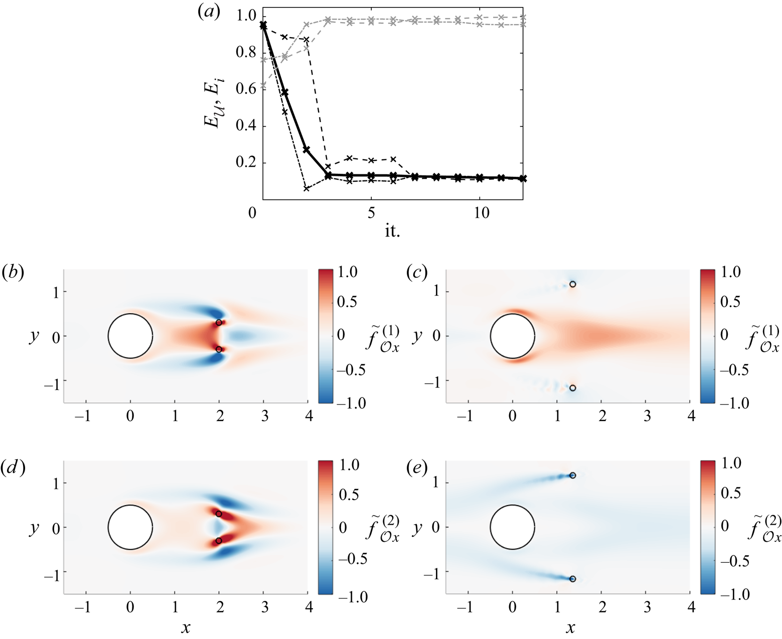
Optimization of the locations of two sensors (initial (b,d) and optimized (c,e) sensors are denoted with open circles) to enhance the reconstruction of the mean velocity field according to (2.16a,b): (a) total residual  $E_{\mathcal {U}}$ (——–) vs the iteration of the optimization procedure;
 $E_{\mathcal {U}}$ here includes the residuals
 $E_{1}$ (– - – -) and
 $E_{2}$ (– – – –) for the first two modes
 $\tilde {\boldsymbol {f}}_{\mathcal {U}}^{(i)}$ (
 $N_{\mathcal {U}}=2$). The residuals
 $E_{3}$ (– - – -, grey) and
 $E_{4}$ (– – – –, grey) for the third and fourth modes are also reported. The streamwise component of the first two dominant modes
 $\tilde {\boldsymbol {f}}_{\mathcal {O}}^{(i)}$ are reported in the second and third rows for the initial (b,d) and optimized (c,e) networks.

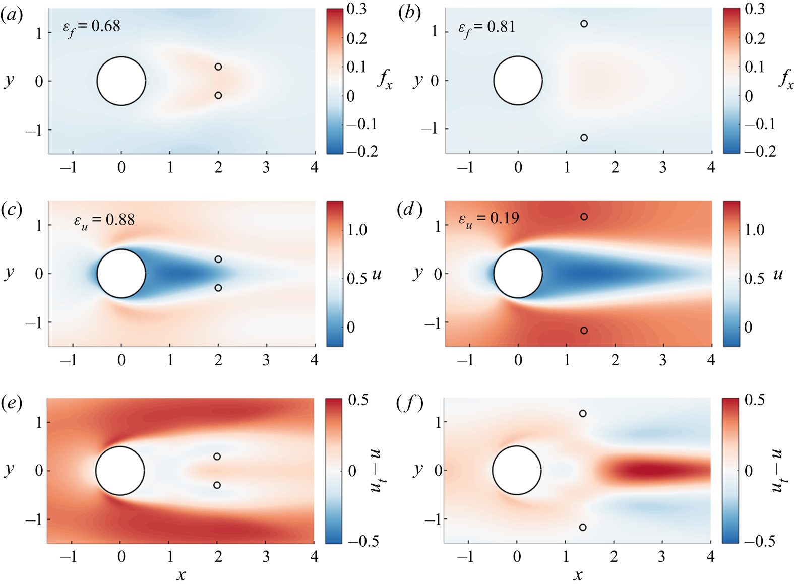
Optimization of the locations of two sensors to enhance the reconstruction of the mean velocity field according to (2.16a,b): results for the initial (left column) and optimized (right column) networks of figure 5. The streamwise component of the assimilated forcing and mean velocity field obtained with these sensor networks are reported in the first and second rows. The discrepancy fields between the assimilated and true velocity fields are also reported in the third row. The reconstruction errors  $\varepsilon _{f}$ and
 $\varepsilon _{u}$ in (3.1a,b) are indicated for the two networks.

As two sensors are used, we choose to evaluate the residual  $E_{\mathcal {U}}$ in (2.16a,b) with
 $N_{\mathcal {U}}$=2, i.e. we only aim to correctly represent the two most dominant modes
 $\tilde {\boldsymbol {f}}_{\mathcal {U}}^{(i)}$ of figures 3(a) and 3(c) in the basis
 $(\tilde {\boldsymbol {f}}_{\mathcal {O}}^{(i)})_{i \in \{ 1,2,\ldots ,N_{\mathcal {O}}\}}$. As may be inferred from figure 5(a), the value of
 $E_{\mathcal {U}}$ is close to the maximum possible value
 $1$ (
 $0.96$) for the first-guess sensors. This indicates that the corresponding eigenforcings
 $\tilde {\boldsymbol {f}}_{\mathcal {O}}^{(i)}$, which are illustrated in figures 5(b) and 5(d), do not form an appropriate basis for the first two modes
 $\tilde {\boldsymbol {f}}_{\mathcal {U}}^{(i)}$. Rather, they seem more adequate for representing the third and fourth modes
 $\tilde {\boldsymbol {f}}_{\mathcal {U}}^{(i)}$ that specifically enable an adjustment of the recirculation region. The minimization of the total residual
 $E_{\mathcal {U}}$ is performed in
 $12$ iterations, each of them requiring the eigendecomposition of the operator
 $\boldsymbol{\mathcal {H}}^{{L}}_{\mathcal {O}}|_{\boldsymbol {q}_{{b}}}$ in (2.9) evaluated at the base flow, reaching the value
 $E_{\mathcal {U}}=0.11$. The sensors of the thus obtained optimized network have been moved away from the
 $y$-axis, enabling a much better representation of the first two modes
 $\tilde {\boldsymbol {f}}_{\mathcal {U}}^{(i)}$, as illustrated by the similarities between figures 3(a) and 3(c), on the one hand, and 5(c) and 5(e), on the other hand. However, this was achieved at the expense of the representation of the third and fourth modes
 $\tilde {\boldsymbol {f}}_{\mathcal {U}}^{(i)}$, as confirmed by the overall increase in the associated residuals
 $E_3$ and
 $E_4$ in figure 5(a). The sensor placement procedure has thus traded the ability to adjust the recirculation bubble for a better identification of more energetic variations in the mean velocity field outside of the wake, as confirmed below.
The assimilated flows obtained with the initial and optimized sensor networks through the data assimilation procedure of § 2.5 are illustrated in figure 6. In both cases, the reconstructed forcing appears far from the true one in figure 2(b), with associated error  $\varepsilon _{f}=0.68$ and
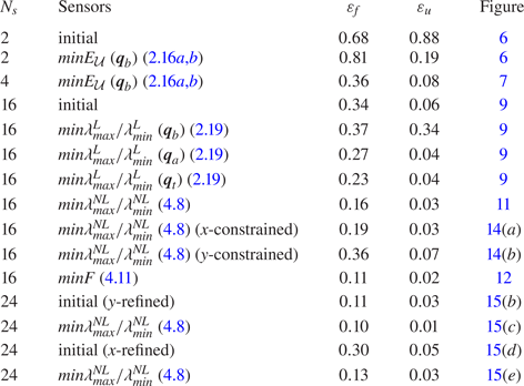
 $\varepsilon _{f}=0.81$ in (3.1a,b) for the initial and optimized networks, respectively. These errors are also reported in table 1 for all cases in this study. The improvement with respect to the first-guess forcing
 $\boldsymbol {f}_{{b}}=\boldsymbol {0}$ thus remains limited. This is in line with the above discussion on figure 4 and the required number of sensors to satisfactorily solve the inverse problem. Concerning the reconstruction of the mean velocity field, the performances of the initial sensors are also poor, as the discrepancies between the assimilated and true fields are quantified as
 $\varepsilon _{u}=0.88$. While the prediction of the extent of the recirculation region has been much improved compared with the base flow, as might have been anticipated, the assimilated flow significantly underestimates the intensity of the mean velocity in the rest of the domain. Interestingly, as may be inferred from the comparison between figures 3(b), 3(d) and 6(e), the discrepancies between this assimilated flow and the true one bear strong similarities with the mean velocity perturbations that are induced by the two dominant modes
 $\tilde {\boldsymbol {f}}_{\mathcal {U}}^{(i)}$, which are not well captured by this sensor network. The optimized sensors achieve much better performances in terms of mean velocity reconstruction, with
 $\varepsilon _{u}=0.19$. It may be worth emphasizing that this drastic improvement was obtained despite a deterioration in the forcing estimation compared with the use of the initial sensors. Similarly, while it was noticed above that the third and fourth modes
 $\tilde {\boldsymbol {f}}_{\mathcal {U}}^{(i)}$ were less satisfactorily represented with the optimized sensors than with the initial ones, the remaining discrepancies between the assimilated and true mean velocity fields in figure 6(f) seem very similar in shape to the velocity variations induced by the third mode in figure 3(f). The errors are indeed mainly concentrated in the cylinder wake due to the still overestimated recirculation length with the optimized sensors. All these findings seem to support the relevance and efficiency of the present sensor placement procedure to enhance the reconstruction of the mean velocity field.
Reconstruction results for the different sensor networks in this study;  $N_{{s}}$ refers to the number of sensors, the sensor networks correspond either to initial arrangements or have been optimized through one of the sensor placement criteria. The errors
 $\varepsilon _f$ and
 $\varepsilon _u$ in (3.1a,b) for the assimilated flows obtained with the different networks are provided, along with the figure numbers for the corresponding fields. For the linear sensor placement criteria (2.16a,b) and (2.19), the reference flow around which linearizations are performed is also specified among the base flow (
 $\boldsymbol {q}_{{b}}$), the assimilated flow obtained with the initial
 $16$ sensors (
 $\boldsymbol {q}_{{a}}$) or the true flow (
 $\boldsymbol {q}_{{t}}$).

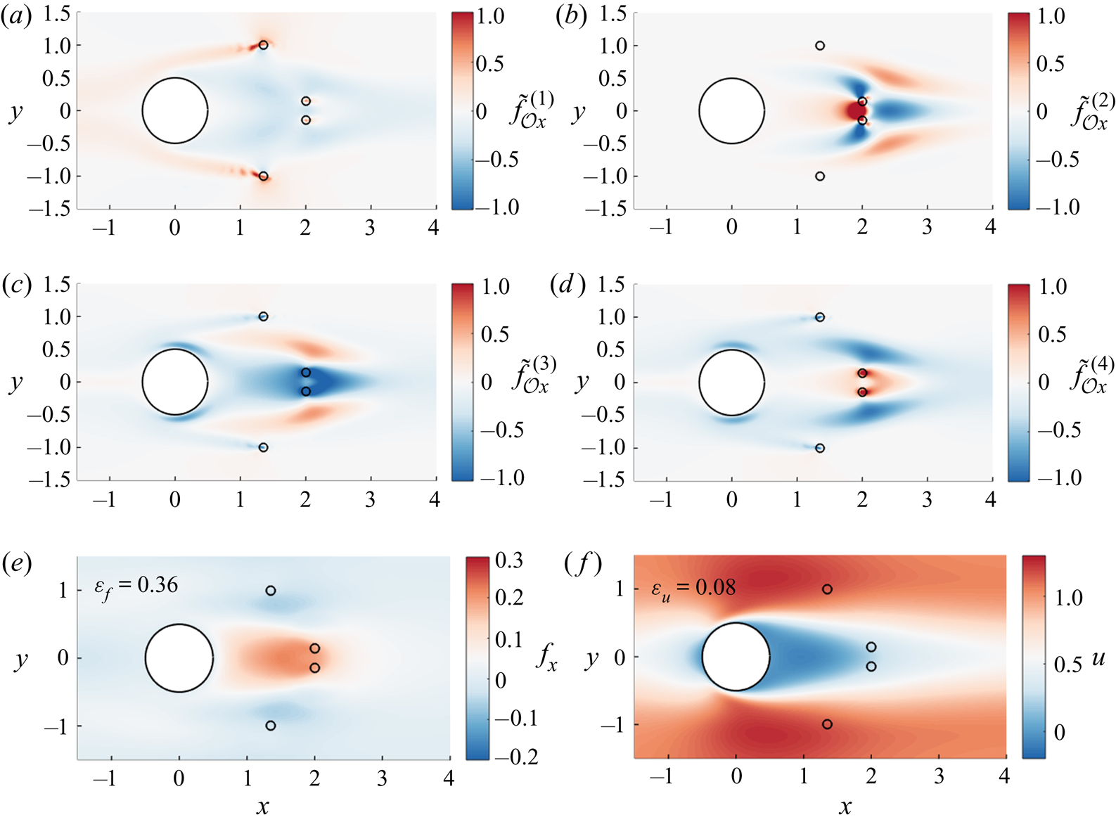
The criterion (2.16a,b) is finally applied to the determination of appropriate locations for four sensors. Figure 7 directly reports results obtained with the optimized configuration, the first-guess network having been formed by the combination of the initial and optimized arrangements of the previous two-sensor case, aiming to correctly reconstruct both the recirculation bubble and outside of the wake region. The present optimized four-sensor network was optimized to correctly infer the  $N_{\mathcal {U}}=4$ modes
 $\tilde {\boldsymbol {f}}_{\mathcal {U}}^{(i)}$ in figure 3, reaching the value
 $0.17$ for the total residual
 $E_{\mathcal {U}}$. The shape of these eigenforcings may indeed be visually identified in the modes
 $\tilde {\boldsymbol {f}}_{\mathcal {O}}^{(i)}$ which are reported in figures 7(a)–7(d). While the assimilated forcing obtained with this network is still relatively far from the true one, with
 $\varepsilon _{f}=0.36$, the discrepancies between the assimilated and true mean velocity fields are decreased to
 $\varepsilon _{u}=0.08$, with a correct prediction of the flow both in the recirculation region and away from the wake as intended. As evoked in the discussion on figure 4, four sensors appear indeed enough to already have a good agreement with the true mean velocity field. This further confirms the validity of the present linear sensor placement procedure, while it may be worth emphasizing the fact that the latter did not require any information about the true flow, as it was performed considering the base flow only.
Optimized network of four sensors to enhance the reconstruction of the mean velocity field according to (2.16a,b). The corresponding streamwise component of the first four eigenmodes  $\tilde {\boldsymbol {f}}_{\mathcal {O}}^{(i)}$ are reported in (a)–(d), along with the streamwise component of the assimilated forcing (e) and mean velocity field (f) obtained with this network.

3.3. Enhancing the reconstruction of the forcing
From now on, we will focus on the determination of sensor arrangements to enhance the more challenging reconstruction of the forcing, and here apply the sensor placement procedure described in § 2.4, which aims to make all variations in the forcing observable and inducing non-negligible changes in the measurement values. The objective of the sensor placement thus consists in minimizing the ratio  $\lambda ^{{L}}_{{max}}/\lambda ^{{L}}_{{min}}$ in (2.19) which corresponds to the ratio between the maximum and minimum values of the gain
 $G_{\mathcal {O}}$ in observation space (2.8), or equivalently the condition number of the operator
 $\boldsymbol{\mathcal {H}}^{{L}}_{\mathcal {O}}|_{\boldsymbol {q}}$ in (2.9). Based on the results of § 3.2, it is chosen to directly rely on networks with more sensors than in previous numerical experiments in order to obtain relatively correct estimations of the true forcing. In the following, as an initial sensor arrangement, we consider the network formed by
 $16$ equally spaced sensors in the domain
 $[1,3 ] \times [-1,1]$ that is illustrated in figures 9(a) and 9(b). Similarly to § 3.2, the base flow is first chosen as the flow around which linearizations in § 2.2 are performed and the ratio
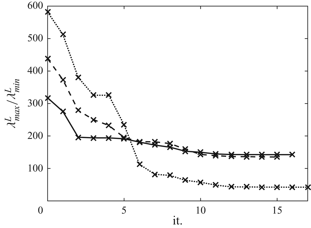
 $\lambda ^{{L}}_{{max}}/\lambda ^{{L}}_{{min}}$ is evaluated. The corresponding optimization procedure is illustrated in figures 8, 9(c) and 9(d). As reported in figure 8 with the dotted line, the ratio
 $\lambda ^{{L}}_{{max}}/\lambda ^{{L}}_{{min}}$ has been decreased by more than one order of magnitude in
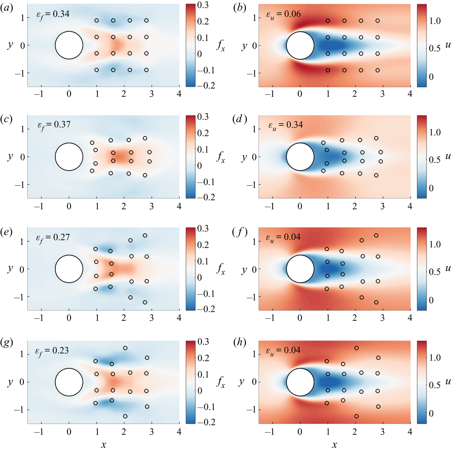
 $17$ iterations. Despite this encouraging result, it appears that the assimilated flow obtained with the thus optimized sensors in figures 9(c) and 9(d) exhibits larger discrepancies with respect to the true flow compared with the use of the initial equally spaced sensors. In particular, the intensity of both the forcing and the mean velocity field is further underestimated with these optimized sensors outside of the wake region. The errors in (3.1a,b) are
 $\varepsilon _{f}=0.34$ and
 $\varepsilon _{u}=0.06$ for the initial sensors, which corresponds to only a small improvement compared with the four-sensor case in § 3.2, while
 $\varepsilon _{f}=0.37$ and
 $\varepsilon _{u}=0.34$ with the optimized sensors. It might be interesting to note that this large alteration in the estimation of the mean velocity field was induced by a comparatively small increase in the error on the forcing. These poorer reconstruction performances point out the limitations of the analysis of § 2.4, and the base flow appears too far from the true one to make the ratio
 $\lambda ^{{L}}_{{max}}/\lambda ^{{L}}_{{min}}$ a relevant indicator for sensor placement. In other words, enhancing the detection of small perturbations induced by variations in the forcing through the linear analysis of § 2.4 is not necessarily appropriate if linearizations are performed around a reference flow that is a too crude estimation of the true one.
Optimization of the locations of  $16$ sensors to enhance the reconstruction of the forcing according to (2.19): ratio
 $\lambda ^{{L}}_{{max}}/\lambda ^{{L}}_{{min}}$ vs the iteration of the optimization procedure when the latter is evaluated at the base flow (dotted line), at the assimilated flow obtained with the initial
 $16$ equally spaced sensors (dashed line) or at the true flow (full line). Assimilated flows obtained with the thus optimized sensors are illustrated in figure 9.

Optimization of the locations of  $16$ sensors to enhance the reconstruction of the forcing according to (2.19): streamwise component of the assimilated forcing (left column) and mean velocity field (right column) obtained with the initial sensor network (first row) and with the optimized sensors when the ratio
 $\lambda ^{{L}}_{{max}}/\lambda ^{{L}}_{{min}}$ is evaluated at the base flow (second row), at the assimilated flow obtained with the initial sensors (third row) or at the true flow (fourth row).

The above results thus motivate the consideration of reference flows that are closer to the true one for the sensor placement criterion (2.19). Starting from the same initial equally spaced network, we now rely on the assimilated flow which was obtained with these sensors in figures 9(a) and 9(b) to evaluate the ratio  $\lambda ^{{L}}_{{max}}/\lambda ^{{L}}_{{min}}$ and perform its minimization, as illustrated in figures 9(e) and 9(f) and figure 8 with the dashed line. Comparisons between these figures and figures 9(c) and 9(d) confirm the impact of nonlinearity in the present inverse problem. Firstly, while the same initial sensor network is employed in both cases, it appears from figure 8 that the value of the ratio
 $\lambda ^{{L}}_{{max}}/\lambda ^{{L}}_{{min}}$ at the beginning of the minimization procedure is significantly affected by the choice of the reference flow around which it is evaluated. In addition, the optimized sensor network that is retrieved in the present case in figures 9(e) and 9(f) differs significantly from the previous one in figures 9(c) and 9(d). Contrary to this previous case, the assimilated flow obtained with the optimized sensors is here closer to the true flow compared with the use of the initial equally spaced network, with
 $\varepsilon _{f}=0.27$ and
 $\varepsilon _{u}=0.04$ (vs
 $\varepsilon _{f}=0.34$ and
 $\varepsilon _{u}=0.06$ for the initial sensors). The remaining discrepancies between assimilated and true flows may be better visualized in figure 13 which will be discussed in § 5.3. It is still possible from figures 9(e) and 9(f) to identify improvements in the assimilated flow compared with the use of the initial sensors, in particular in the subdomain
 $x \in [1,1.5]$, where the forcing exhibits larger positive and negative values which induce an improvement in the mean velocity in the same region with a better estimation of the recirculation length. These encouraging performances could suggest the design of an iterative procedure, where the assimilated flow obtained with the sensor network designed at previous iteration is used to perform the linearizations in § 2.2 and the minimization of the ratio
 $\lambda ^{{L}}_{{max}}/\lambda ^{{L}}_{{min}}$ to get a new sensor arrangement, and then a new assimilated flow for a next iteration. We thus attempted to consider the assimilated flow in figures 9(e) and 9(f) and the corresponding sensors to determine a new optimal arrangement according to (2.19) (results not shown here for the sake of brevity), but the sensor locations were hardly changed during the process, compromising the point of the above mentioned iterative procedure.
The true flow itself is finally considered to perform the minimization of the ratio  $\lambda ^{{L}}_{{max}}/\lambda ^{{L}}_{{min}}$, as reported in figures 9(g) and 9(h) and figure 8 with the full line, still starting from the equally spaced network. The thus obtained optimized sensors are different from those in the two previous cases, further illustrating the impact of nonlinearity. As might have been expected, the assimilated flow obtained with these sensors appears further improved compared with the use of the previously retrieved optimized arrangements, in particular in terms of forcing identification, with
 $\varepsilon _{f}=0.23$ (and
 $\varepsilon _{u}=0.04$). While these results confirm that the minimization of the ratio
 $\lambda ^{{L}}_{{max}}/\lambda ^{{L}}_{{min}}$ is more and more relevant for sensor placement as it is performed around a closer approximation of the true flow, this also further points out the limitations of this approach, as we had to consider the true flow itself to get a significant improvement in the quality of the assimilated flow compared with the use of the initial equally spaced network. These relatively poor performances may be attributed to the fact that all nonlinearities were neglected in the derivations of the criterion (2.19). Accordingly, in order to further improve the estimation of the true flow through optimal sensor placement without having to rely on extra information about the latter besides the available measurements, one may now want to take into account the dependency of the ratio
 $\lambda ^{{L}}_{{max}}/\lambda ^{{L}}_{{min}}$ with respect to the mean flow during its minimization, which is the subject of the following sections.
4. Nonlinear sensor placement strategies
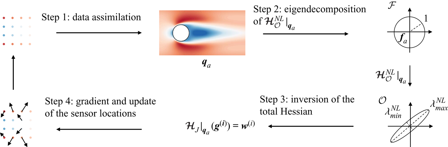
As discussed in § 3, while the linear sensor placement procedure of § 2.3 to specifically enhance the reconstruction of the mean velocity field appeared effective, the methodology of § 2.4 to improve the estimation of the forcing showed some limitations, as it requires a good approximation of the true mean flow of interest to actually provide a better forcing estimate. In §§ 4.1 and 4.2, an extension of this methodology is made, which consists in always evaluating an equivalent of the ratio  $\lambda ^{{L}}_{{max}}/\lambda ^{{L}}_{{min}}$ in (2.19) at the assimilated flow obtained with the current network design during the sensor placement procedure. The sensor locations are adjusted while taking into account all nonlinearities in the data assimilation problem, including the dependency of the ratio
 $\lambda ^{{L}}_{{max}}/\lambda ^{{L}}_{{min}}$ with respect to the current assimilated flow. This is achieved through the development of a second-order adjoint-based procedure, which is also used to design a second nonlinear sensor placement criterion for validation purposes in § 4.3.
4.1. Nonlinear sensor placement for forcing identification
The linear sensor placement procedure of § 2.4 to enhance the estimation of the forcing is here extended to take into account all nonlinearities in the present inverse problem. This is first performed by considering variations  $\delta J$ in the value of the cost function for the data assimilation problem
 $J=\frac {1}{2}\| \boldsymbol {y}-\boldsymbol {h}(\boldsymbol {q})\|_{\mathcal {O}}^{2}+({\alpha }/{2})(\| \boldsymbol {f} \|^{2}_{\mathcal {F}}+ \|\boldsymbol {\nabla } \boldsymbol {f} \|^{2}_{\mathcal {G}} )$ which are induced by perturbations
 $\delta \boldsymbol {f}$ in the forcing
 $\boldsymbol {f}$. The perturbation
 $\delta J$ can be expressed up to second order as
 \begin{equation} \delta J = J(\,\boldsymbol{f}+\delta\boldsymbol{f})-J(\,\boldsymbol{f})\simeq \left\langle \left.\frac{\partial J}{\partial \boldsymbol{f}}\right|_{\boldsymbol{f}},\delta\boldsymbol{f} \right\rangle_{\mathcal{F}}+\frac{1}{2}\langle \boldsymbol{\mathcal {H}}_{J}|_{\boldsymbol{q}}(\delta\boldsymbol{f}), \delta\boldsymbol{f}\rangle_{\mathcal{F}}, \end{equation}
where the first-order term in the right-hand side of (4.1) involves the gradient of  $J$ with respect to the forcing in (2.22), while the second-order contribution involves the Hessian operator
 $\boldsymbol{\mathcal {H}}_{J}|_{\boldsymbol {q}}$. The application of this operator to a forcing vector can be decomposed according to
 \begin{equation} \boldsymbol{\mathcal {H}}_{J}|_{\boldsymbol{q}}(\delta\boldsymbol{f})= \boldsymbol{\mathcal {H}}^{{NL}}_{\mathcal{O}}|_{\boldsymbol{q}}(\delta\boldsymbol{f})+ \alpha(\delta\boldsymbol{f}-\varDelta \delta\boldsymbol{f} ), \end{equation}
where  $\boldsymbol{\mathcal {H}}^{{NL}}_{\mathcal {O}}|_{\boldsymbol {q}}$ refers to the Hessian associated with the observation part of the cost function
 $J$, i.e.
 $\frac {1}{2}\| \boldsymbol {y}-\boldsymbol {h}(\boldsymbol {q})\|_{\mathcal {O}}^{2}$, while the remaining term in (4.2) originates from the penalization contribution. The application of
 $\boldsymbol{\mathcal {H}}^{{NL}}_{\mathcal {O}}|_{\boldsymbol {q}}$ to
 $\delta \boldsymbol {f}$ is performed according to
 \begin{equation} \boldsymbol{\mathcal {H}}^{{NL}}_{\mathcal{O}}|_{\boldsymbol{q}}(\delta\boldsymbol{f}) =\delta \boldsymbol{u}^{{{\dagger}}}=\boldsymbol{\mathcal{R}}|_{\boldsymbol{q}}^{{{\dagger}}} ( \boldsymbol{h}^{{{\dagger}}}(\boldsymbol{h}(\delta \boldsymbol{q})) - \boldsymbol{{P}}\tilde{\boldsymbol{b}}(\boldsymbol{u}^{{{\dagger}}}, \delta \boldsymbol{u}) ), \quad \delta\boldsymbol{q}=\begin{pmatrix} \delta\boldsymbol{u} \\ \delta p \end{pmatrix}=\boldsymbol{\mathcal{R}}|_{\boldsymbol{q}}(\delta \boldsymbol{f}). \end{equation}
Equation (4.3) thus amounts to evaluating the variation  $\delta \boldsymbol {u}^{{\dagger} }$ in the adjoint velocity field
 $\boldsymbol {u}^{{\dagger} }=\boldsymbol {\mathcal {R}}|_{\boldsymbol {q}}^{{\dagger} } (\boldsymbol {h}^{{\dagger} }(\boldsymbol {h}(\boldsymbol {q})-\boldsymbol {y}))$ which was introduced for the data assimilation problem (see § 2.5). The computation of
 $\delta \boldsymbol {u}^{{\dagger} }$ first requires the application of the resolvent operator
 $\boldsymbol {\mathcal {R}}|_{\boldsymbol {q}}$ to
 $\delta \boldsymbol {f}$, and then that of its adjoint forced by the combination of the observation term
 $\boldsymbol {h}^{{\dagger} }(\boldsymbol {h}(\delta \boldsymbol {q}))$ and the quadratic contribution
 $\tilde {\boldsymbol {b}}(\boldsymbol {u}^{{\dagger} }, \delta \boldsymbol {u})$. The latter arises from the convection term in the RANS equations (2.1) and is defined as
 \begin{equation} \tilde{\boldsymbol{b}}(\boldsymbol{u}^{{{\dagger}}}, \delta \boldsymbol{u}) =\boldsymbol{u}^{{{\dagger}}}\boldsymbol{\cdot} (\boldsymbol{\nabla} \delta\boldsymbol{u})^{\top}-(\delta\boldsymbol{u}\boldsymbol{\cdot} \boldsymbol{\nabla} )\boldsymbol{u}^{{{\dagger}}}. \end{equation}
It is worth noting that, by removing this contribution from (4.3), one recovers the definition of the operator  $\boldsymbol{\mathcal {H}}^{{L}}_{\mathcal {O}}|_{\boldsymbol {q}}$ in (2.9) that was associated with the gain in observation space in § 2.2. The superscript
 ${NL}$ is thus employed to emphasize the presence of this supplementary term in
 $\boldsymbol{\mathcal {H}}^{{NL}}_{\mathcal {O}}|_{\boldsymbol {q}}$. Equation (4.3) forms the second-order adjoint model that is associated with the RANS equations (2.1) (Wang et al. Reference Wang, Navon, Le Dimet and Zou1992; Le Dimet et al. Reference Le Dimet, Ngodock, Luong and Verron1997, Reference Le Dimet, Navon and Daescu2002). As the second-order contribution (4.4) is similar to terms that are already present in the first-order adjoint model (2.12), its implementation is straightforward in the present case.
Of particular interest to quantify the uncertainties in the assimilated flow is to express the variation  $\delta J$ for the latter. In this case, the first-order contribution vanishes, and (4.1) for perturbations
 $\delta \boldsymbol {f}$ around the assimilated forcing
 $\boldsymbol {f}_{{a}}$ and mean flow
 $\boldsymbol {q}_{{a}}$ becomes
 \begin{equation} \delta J \simeq \tfrac{1}{2}\langle \boldsymbol{\mathcal {H}}_{J}|_{\boldsymbol{q}_{{a}}}(\delta\boldsymbol{f}), \delta\boldsymbol{f}\rangle_{\mathcal{F}}. \end{equation}
In the following, similarly to § 2.4, we aim to design sensor networks that are able to distinguish between all possible variations around the assimilated forcing  $\boldsymbol {f}_{{a}}$. To this end, we first consider as forcing perturbations the eigenmodes
 $\boldsymbol {f}^{(i)}_{\mathcal {O}}$ of
 $\boldsymbol{\mathcal {H}}^{{NL}}_{\mathcal {O}}|_{\boldsymbol {q}_{a}}$. The latter therefore verify
 \begin{equation} \boldsymbol{\mathcal {H}}^{{NL}}_{\mathcal{O}}|_{\boldsymbol{q}_{{a}}} (\,\boldsymbol{f}^{(i)}_{\mathcal{O}})=\boldsymbol{u}_{\mathcal{O}}^{{{\dagger}}\,(i)} =\lambda^{{NL}}_{i} \boldsymbol{f}^{(i)}_{\mathcal{O}}, \quad \|\,\boldsymbol{f}^{(i)}_{\mathcal{O}} \|^{2}_{\mathcal{F}}=1, \quad \boldsymbol{u}_{\mathcal{O}}^{(i)}=\boldsymbol{R} \boldsymbol{\mathcal{R}}|_{\boldsymbol{q}_{{a}}} (\,\boldsymbol{f}_{\mathcal{O}}^{(i)}), \end{equation}
where  $\lambda ^{{NL}}_{i}$ is the eigenvalue of
 $\boldsymbol{\mathcal {H}}^{{NL}}_{\mathcal {O}}|_{\boldsymbol {q}_{{a}}}$ that is associated with
 $\boldsymbol {f}^{(i)}_{\mathcal {O}}$, which is normalized to
 $1$, with relative mean velocity perturbation
 $\boldsymbol {u}_{\mathcal {O}}^{(i)}$. For such eigenmodes, (4.5) becomes
 \begin{equation} \delta J \simeq \frac{1}{2}\lambda_{i}^{{NL}} +\frac{\alpha}{2}(1+ \|\boldsymbol{\nabla} \boldsymbol{f}^{(i)}_{\mathcal{O}} \|^{2}_{\mathcal{G}}). \end{equation}
Putting aside the contribution in (4.7) that is weighted by  $\alpha$ and comes from the regularization part in
 $J$, the interpretation of the eigenforcings
 $\boldsymbol {f}^{(i)}_{\mathcal {O}}$ may be as follows. Eigenforcings with small eigenvalues do not entail significant perturbations in the observation part of the cost function according to
 $\delta J \simeq \frac {1}{2}\lambda _{i}^{{NL}}$ and are thus hardly differentiable from the assimilated forcing
 $\boldsymbol {f}_{{a}}$. In other words, the assimilated forcing is highly uncertain in the space spanned by such eigenmodes. On the contrary, eigenforcings that are associated with large eigenvalues correspond to states which have been accurately captured from the observations. The mapping from the forcing space to the observation one through
 $\boldsymbol{\mathcal {H}}^{{NL}}_{\mathcal {O}}|_{\boldsymbol {q}_{{a}}}$ is illustrated in the right part of figure 10, assuming a two-dimensional forcing space for the sake of illustration. Similarly to § 2.4, in order to design sensor networks that are able to differentiate between all possible variations in the assimilated forcing, the sensor placement problem is here formulated as
 \begin{equation} min_{(\boldsymbol{x}_{{s}}^{(k)})_{k \in \{ 1,2,\ldots,N_{{s}}\}}} \frac{\lambda^{{NL}}_{{max}}}{\lambda^{{NL}}_{{min}}}, \end{equation}
where  $\lambda ^{{NL}}_{{max}}$ and
 $\lambda ^{{NL}}_{{min}}$ correspond to the largest and smallest eigenvalues of
 $\boldsymbol{\mathcal {H}}^{{NL}}_{\mathcal {O}}|_{\boldsymbol {q}_{{a}}}$. It may be worth emphasizing that (4.8) forms a meta-optimization problem, as the ratio
 $\lambda ^{{NL}}_{{max}}/\lambda ^{{NL}}_{{min}}$ has always to be evaluated at the assimilated flow for the current sensor network in order to remain consistent with the above analysis. In other words, each time the sensor locations are updated during the minimization of
 $\lambda ^{{NL}}_{{max}}/\lambda ^{{NL}}_{{min}}$, it is first required to solve the data assimilation problem (2.21a,b) with the measurements at the new sensor locations. When evaluating sensitivities, this has to be taken into account through the consideration as an equality constraint of the first-order optimality condition
 $\partial J/\partial \boldsymbol {f}|_{\boldsymbol {f}_{{a}}}=\boldsymbol {0}$ using (2.22). The full Lagrangian that may be introduced to solve (4.8) is given in (C1). The gradient of an eigenvalue
 $\lambda ^{{NL}}_{i}$ as involved in (4.6a–c) and (4.8) with respect to the location of the
 $k$th sensor can be obtained through
 \begin{equation} \frac{\partial \lambda^{{NL}}_{i}}{\partial \boldsymbol{x}_{{s}}^{(k)}}= 2 ( \boldsymbol{\nabla} \boldsymbol{u}_{\mathcal{O}}^{(i)}(\boldsymbol{x}_{{s}}^{(k)}) )^{\top} \boldsymbol{u}_{\mathcal{O}}^{(i)}(\boldsymbol{x}_{{s}}^{(k)})+ \boldsymbol{\nabla} ( ( \boldsymbol{u}_{{a}}-\boldsymbol{y}^{(k)} )^{\top} \boldsymbol{v}^{(i)} )(\boldsymbol{x}_{{s}}^{(k)}). \end{equation}
Similarly to § 2.4, once (4.9) is applied to  $\lambda ^{{NL}}_{{max}}$ and
 $\lambda ^{{NL}}_{{min}}$, one can get the gradient of their ratio. The first contribution in the sensitivity (4.9), which involves the mean velocity
 $\boldsymbol {u}_{\mathcal {O}}^{(i)}$ in (4.6a–c), is similar to the gradient
 $\partial \lambda ^{{L}}_{i}/\partial \boldsymbol {x}_{{s}}^{(k)}$ in (2.20). It reflects the direct dependency of
 $\boldsymbol{\mathcal {H}}^{{NL}}_{\mathcal {O}}|_{\boldsymbol {q}_{{a}}}$ with respect to the observation locations. On the other hand, the second term in (4.9) takes into account the dependency of
 $\boldsymbol{\mathcal {H}}^{{NL}}_{\mathcal {O}}|_{\boldsymbol {q}_{{a}}}$ with respect to the assimilated flow, which varies as the sensors are moved. It may be noticed that this contribution involves the gradient of the assimilated mean velocity field
 $\boldsymbol {u}_{{a}}$, but also that of the measurements
 $\boldsymbol {y}$ at the sensor locations. The present sensor placement procedure thus requires the possibility of performing mean velocity gradient measurements. However, it is believed that this does not necessarily prevent the application of this methodology to practical settings, as well-known experimental techniques such as the hot-wire method or laser Doppler anemometry can give access to velocity gradients.
Summary of the iterative procedure to minimize the ratio  $\lambda ^{{NL}}_{{max}}/\lambda ^{{NL}}_{{min}}$ in (4.8). For the sake of illustration only, the mapping from the forcing space to the observation one through the operator
 $\boldsymbol{\mathcal {H}}^{{NL}}_{\mathcal {O}}|_{\boldsymbol {q}_{{a}}}$ in (4.3) is depicted assuming a two-dimensional forcing space.

The most computationally demanding step in the evaluation of the gradient (4.9) is to obtain the mean velocity field  $\boldsymbol {v}^{(i)}$. While proper definitions and derivations are provided in Appendix C, the evaluation of
 $\boldsymbol {v}^{(i)}$ mainly involves the inversion of a system of the form
 \begin{equation} \boldsymbol{\mathcal {H}}_{J}|_{\boldsymbol{q}_{{a}}}(\boldsymbol{g}^{(i)})=\boldsymbol{w}^{(i)}, \end{equation}
where the unknown pseudo-forcing  $\boldsymbol {g}^{(i)}$ allows us to determine
 $\boldsymbol {v}^{(i)}$ according to (C2), and the right-hand side
 $\boldsymbol {w}^{(i)}$ is defined in (C3)–(C5). The whole procedure to minimize the ratio
 $\lambda ^{{NL}}_{{max}}/\lambda ^{{NL}}_{{min}}$ is summarized in § 4.2.
4.2. Resolution method
The meta-optimization problem (4.8) is solved with the nonlinear conjugate gradient method, as in the previous sensor placement procedures. This section summarizes the four successive steps, sketched in figure 10, that allow us to compute the gradient of the ratio  $\lambda ^{{NL}}_{{max}} /\lambda ^{{NL}}_{{min}}$ with respect to the sensor locations. Details about numerical implementation are also provided in the following.
The first step is to solve the data assimilation problem (2.21a,b) based on the measurements of the true flow at the current sensor locations. This iterative method, detailed in § 2.5, requires multiple applications of the resolvent  $\boldsymbol {\mathcal {R}}|_{\boldsymbol {q}}$ and adjoint
 $\boldsymbol {\mathcal {R}}|_{\boldsymbol {q}}^{{\dagger} }$ operators, defined in (2.6a,b) and (2.11). They require us to solve linear problems involving the linearized RANS operator
 $(\partial \boldsymbol {\mathcal {N}}/\partial \boldsymbol {q})|_{\boldsymbol {q}}$ and its adjoint
 $((\partial \boldsymbol {\mathcal {N}}/\partial \boldsymbol {q})|_{\boldsymbol {q}})^{{\dagger} }$. With that aim, the mean flow
 $\boldsymbol {q}$ at a given iteration of the data assimilation procedure is first used to assemble these discrete operators and their inversion is then performed with a sparse direct solver. The output of data assimilation is an assimilated forcing
 $\boldsymbol {f}_{{a}}$, the corresponding mean flow
 $\boldsymbol {q}_{{a}}$ and the adjoint velocity field
 $\boldsymbol {u}^{{\dagger} }_{{a}}$, solution to the adjoint problem (2.23) at the end of the data assimilation procedure.
The second step is the eigenvalue decomposition of the observation Hessian  $\boldsymbol{\mathcal {H}}^{{NL}}_{\mathcal {O}}|_{\boldsymbol {q}_{{a}}}$ defined in (4.3) for the assimilated mean flow
 $\boldsymbol {q}_{{a}}$ obtained from step 1. It is here performed with an Arnoldi method (Saad Reference Saad2011) that only requires the application of the observation Hessian operator at each iteration of the algorithm. According to (4.3), this application consists in successively applying the resolvent operator
 $\boldsymbol {\mathcal {R}}|_{\boldsymbol {q}_{{a}}}$ and its adjoint
 $\boldsymbol {\mathcal {R}}|_{\boldsymbol {q}_{{a}}}^{{\dagger} }$ (which are thus always evaluated around the assimilated flow
 $\boldsymbol {q}_{{a}}$) to various vectors. In particular, the adjoint velocity
 $\boldsymbol {u}^{{\dagger} }_{{a}}$ obtained in step 1 is involved in the definition of the vector to which the adjoint resolvent applies. The outputs of the eigendecomposition are the maximal
 $\lambda ^{{NL}}_{{max}}$ and minimal
 $\lambda ^{{NL}}_{{min}}$ eigenvalues and the associated eigenforcings
 $\boldsymbol {f}_{\mathcal {O}}^{{max}}$ and
 $\boldsymbol {f}_{\mathcal {O}}^{{min}}$. In addition, the mean velocity variations
 $\boldsymbol {u}_{\mathcal {O}}^{{max}}$ and
 $\boldsymbol {u}_{\mathcal {O}}^{{min}}$ are obtained by applying the resolvent operator to the corresponding eigenforcings according to (4.6a–c).
The third step consists in solving the linear problem (4.10) twice (for both maximum and minimum eigenmodes), where the right-hand side  $\boldsymbol {w}^{(i)}$ is built based on the eigenvalues and eigenmodes from previous step, as detailed in Appendix C and (C3)–(C5). This requires the inversion of the total Hessian
 $\boldsymbol{\mathcal {H}}_{J}|_{\boldsymbol {q}_{{a}}}$, defined in (4.2) and (4.3), that is here performed with the generalized minimal residual method (GMRES) (Cioaca, Sandu & de Sturler Reference Cioaca, Sandu and de Sturler2013). Each iteration of the GMRES algorithm requires the inversions of the tangent linear RANS equations and of their adjoint, similarly to the eigendecomposition in step 2, as well as the application of the Laplacian operator (regularization term in (4.2)).
The fourth (and last) step is the determination of the gradient of the ratio  $\lambda ^{{NL}}_{{max}}/\lambda ^{{NL}}_{{min}}$ with respect to the sensor locations, based on the solutions from previous step (pseudo-forcing
 $\boldsymbol {g}^{(i)}$ in (4.10)) and (C2) and (4.9). It then allows us to update the sensor locations according to the nonlinear conjugate gradient method.
4.3. Optimal forcing reconstruction
In the present case, the most ideal and straightforward criterion for optimal sensor placement could be formulated as identifying sensor locations in order to minimize the discrepancies between the assimilated forcing  $\boldsymbol {f}_{{a}}$ and the true one
 $\boldsymbol {f}_{{t}}$, namely
 \begin{equation} min_{(\boldsymbol{x}_{{s}}^{(k)})_{k \in \{ 1,2,\ldots,N_{{s}}\}}} \{ F=\tfrac{1}{2}\|\,\boldsymbol{f}_{{a}} - \boldsymbol{f}_{{t}}\|^{2}_{\mathcal{F}} \}. \end{equation}
An obvious flaw of the criterion (4.11) is that the latter requires the unknown of the present data assimilation problem itself  $\boldsymbol {f}_{{t}}$, which prevents its use in practical applications. However, (4.11) will be here employed to identify the best achievable forcing reconstruction for a given number of sensors, which will then be compared to the performances of the previously introduced sensor placement procedures. Similarly as in § 4.1, as the criterion (4.11) involves the assimilated forcing
 $\boldsymbol {f}_{{a}}$, it forms a meta-optimization problem whose resolution first requires solving of the data assimilation problem (2.21a,b) (step 1 in § 4.2). The gradient of the cost function
 $F$ in (4.11) with respect to the
 $k$th sensor location is given by
 \begin{equation} \frac{\partial F}{\partial \boldsymbol{x}_{{s}}^{(k)}}= \boldsymbol{\nabla} ( ( \boldsymbol{u}_{{a}}-\boldsymbol{y}^{(k)} )^{\top} \boldsymbol{v} )(\boldsymbol{x}_{{s}}^{(k)}), \end{equation}
where the mean velocity  $\boldsymbol {v}$ is obtained from
 $\boldsymbol {v}=\boldsymbol {R}\boldsymbol {\mathcal {R}}|_{\boldsymbol {q}_{{a}}}(\boldsymbol {g})$, where the forcing
 $\boldsymbol {g}$ is computed through the inversion of
 \begin{equation} \boldsymbol{\mathcal {H}}_{J}|_{\boldsymbol{q}_{a}}(\boldsymbol{g})= \boldsymbol{f}_{{t}}-\boldsymbol{f}_{{a}}. \end{equation}
The evaluation of the gradient (4.12) is thus performed in a similar way to step 3 in § 4.2, although with a different right-hand side for the inversion of the total Hessian  $\boldsymbol{\mathcal {H}}_{J}|_{\boldsymbol {q}_{a}}$.
5. Application of nonlinear sensor placement
5.1. Minimization of the ratio  $\lambda ^{{NL}}_{{max}}/\lambda ^{{NL}}_{{min}}$ (4.8)

The nonlinear sensor placement strategies of § 4 are now applied to the optimization of the locations of  $16$ sensors, as already considered in § 3.3. Starting from the same initial equally spaced network as in figures 9(a) and 9(b), the criterion (4.8) is first employed here, which is illustrated in figure 11. This sensor placement procedure consists in minimizing the ratio
 $\lambda ^{{NL}}_{{max}}/\lambda ^{{NL}}_{{min}}$ in order to make all variations around the assimilated forcing perceptible in the observation term of the cost function
 $J$ for the data assimilation problem (2.21a,b). As reported in figure 11(a), this meta-optimization problem is here solved in
 $6$ main iterations, each of these iterations first requiring minimizing
 $J$ with the measurements that are provided at the current sensor locations (see figure 11b) to obtain the corresponding assimilated flow (step 1 in § 4.2). Comparisons between the assimilated flow obtained with the present optimized sensors and those in § 3.3, which were retrieved through the linear criterion (2.19) and the minimization of the ratio
 $\lambda ^{{L}}_{{max}}/\lambda ^{{L}}_{{min}}$ when evaluated around various reference flows, will be facilitated through figure 13 (see also table 1). However, it may be already inferred from the comparison between figures 11(c) and 11(d) and figure 9 that the present optimized sensors enable a significantly better estimation of the forcing compared with all previously considered networks, in particular around
 $y=\pm 1$. The corresponding errors in (3.1a,b) are
 $\varepsilon _f=0.16$ and
 $\varepsilon _u=0.03$, confirming the improved performances compared with previous cases, both in terms of forcing and mean velocity field reconstruction.
Optimization of the locations of  $16$ sensors to enhance the reconstruction of the forcing according to (4.8). (a) Ratio
 $\lambda ^{{NL}}_{{max}}/\lambda ^{{NL}}_{{min}}$ vs the iteration of the main optimization procedure, the minimization of the cost function
 $J$ in (2.21a,b) is reported in (b) with increasing grey scale for the outer iterations. The streamwise component of the assimilated (c) forcing and (d) mean velocity field retrieved with the thus obtained optimized sensors are also reported.

5.2. Best achievable forcing reconstruction
In order to get the best achievable estimation of the forcing with  $16$ sensors, the criterion (4.11) which is based on the minimization of the discrepancies between the assimilated and true forcings is now considered, as illustrated in figure 12. The associated meta-optimization problem is here solved in only
 $3$ main iterations, and the thus obtained optimized sensors allow us, based on the knowledge of the true forcing itself, to outperform all previous sensor networks, with
 $\varepsilon _f=0.11$ and
 $\varepsilon _u=0.02$ for the corresponding assimilated flow. Compared with the previous case in figure 11, the sensor placement procedure seems to have further improved the flow estimation around the
 $y$-axis.
Optimization of the locations of  $16$ sensors to enhance the reconstruction of the forcing according to (4.11). (a) Discrepancies between the assimilated and true forcings
 $F$ vs the iteration of the main optimization procedure, the minimization of the cost function
 $J$ in (2.21a,b) is reported in (b) with increasing grey scale for the outer iterations. The streamwise component of the assimilated (c) forcing and (d) mean velocity field retrieved with the thus obtained optimized sensors are also reported.

5.3. Comparisons with linear approaches
Figure 13 reports the errors between the true and assimilated forcings that are obtained with all previously discussed 16-sensor networks. It might be worth recalling that all optimized sensor networks in figures 13(b)–13(f) were obtained starting from the equally spaced network of figure 13(a). Figure 13 clearly illustrates the superiority of the nonlinear sensor placement procedures (figures 13e and 13f) over the linear sensor placement (2.19) for forcing identification (figures 13b–13d). Interestingly, the optimized sensor network obtained through the nonlinear criterion (4.8) based on the minimization of  $\lambda ^{{NL}}_{{max}}/\lambda ^{{NL}}_{{min}}$ in figure 13(e) is similar to that in figure 13(d) which was retrieved from the linear criterion (2.19) when
 $\lambda ^{{L}}_{{max}}/\lambda ^{{L}}_{{min}}$ is evaluated at the true flow. It may be worth emphasizing that the nonlinear criterion (4.8) only required measurements of the true mean velocity and of its gradient at the sensor locations and still outperformed the linear criterion (2.19) in this most favourable case for the latter. In addition, the assimilated flow obtained through the application of (4.8) appears relatively close to the best achievable reconstruction in figure 13(f) which was identified through (4.11).
Discrepancy fields between the true forcing and assimilated forcings obtained with previously designed 16-sensor networks. (a) Initial network, (b)–(d) optimized networks obtained through the minimization of the ratio  $\lambda ^{{L}}_{{max}}/\lambda ^{{L}}_{{min}}$ in (2.19) evaluated at (b) the base flow, (c) the assimilated flow obtained with the initial sensors or (d) the true flow. (e) Optimized network obtained through the minimization of the ratio
 $\lambda ^{{NL}}_{{max}}/\lambda ^{{NL}}_{{min}}$ in (4.8), (f) optimized network obtained through the minimization of
 $F$ in (4.11). The gradient
 $\partial (\lambda ^{{NL}}_{{max}}/\lambda ^{{NL}}_{{min}})/\partial \boldsymbol {x}_{{s}}$ at the beginning and the end of the corresponding sensor placement procedure is reported in (a) and (e) respectively (black arrows).

However, these better reconstruction results obtained through the nonlinear criterion (4.8) should be contrasted with the significant increase in computational cost compared with its linear counterpart (2.19). The CPU times to perform one iteration of the various procedures that have been applied to the above-discussed 16-sensor case are reported in table 2. The linear criterion (2.19), as with all the linear approaches in § 2, only relies on the eigendecomposition of the operator  $\boldsymbol{\mathcal {H}}^{{L}}_{\mathcal {O}}|_{\boldsymbol {q}}$ in (2.9) to evaluate the ratio
 $\lambda ^{{L}}_{{max}}/\lambda ^{{L}}_{{min}}$ and its gradient with respect to the sensor locations, which here corresponds to a computational cost that is equivalent to ten times the integration of the RANS equations (2.1). On the other hand, its nonlinear counterpart (4.8) requires, in addition, solution of the data assimilation problem (2.21a,b) to get the ratio
 $\lambda ^{{NL}}_{{max}}/\lambda ^{{NL}}_{{min}}$ (step 1) and inversion of the total Hessian
 $\boldsymbol{\mathcal {H}}_{J}|_{\boldsymbol {q}_{a}}$ according to (4.10) to compute its gradient with respect to the sensor locations (step 3). While this last step has similar requirements in terms of computational cost as the eigendecomposition of
 $\boldsymbol{\mathcal {H}}^{{NL}}_{\mathcal {O}}|_{\boldsymbol {q}_{{a}}}$ in (4.3) (step 2), the data assimilation step is roughly ten times more demanding, and dominates the computational effort for this sensor placement procedure. The same applies to the best forcing identification through the minimization of
 $F$ in (4.11). Overall, the present nonlinear sensor placement procedures may thus be ten times more expensive than linear approaches in the present case. However, in the case where this supplementary computational cost is affordable, the benefits and better performances of nonlinear sensor placement may appear sufficiently substantial to support their use.
Normalized CPU time  $T_{{CPU}}/T_{{t}}$, where
 $T_{{t}}$ refers to the CPU time to compute the true flow through the RANS equations, for the different steps to perform in one iteration of the sensor placement procedures that are applied in figure 13. These steps correspond to solving the data assimilation problem (2.21a,b) (step 1), computing the eigendecomposition of
 $\boldsymbol{\mathcal {H}}^{{L}}_{\mathcal {O}}|_{\boldsymbol {q}}$ in (2.9) or
 $\boldsymbol{\mathcal {H}}^{{NL}}_{\mathcal {O}}|_{\boldsymbol {q}_{{a}}}$ in (4.3) (step 2) or inverting the total Hessian
 $\boldsymbol{\mathcal {H}}_{J}|_{\boldsymbol {q}_{a}}$ according to (4.10) or (4.13) (step 3).

As the CPU times in table 2 are reported for a 16-sensor network only, one may wonder if these values would vary with respect to the number of sensors. Due to the use of adjoint-based techniques, steps 1 and 3 in table 2 are not significantly affected by the number of sensors  $N_{{s}}$. However, the computational cost for the eigendecomposition that is performed in step 2 is directly determined by the size of the sensor network, and varies linearly with
 $2N_{{s}}$, i.e. the number of non-zero eigenvalues. For networks with more than
 $100$ sensors, the computational cost for this eigendecomposition could thus become similar to that for the data assimilation step. This could be circumvented by considering alternative sensor placement formulations, as discussed in § 2.4.
5.4. Constraining the sensor placement
Aside from numerical considerations, the potentialities of sensor placement would be ultimately determined by the degree of freedom that is offered by the experimental setting. Firstly, specifically concerning the present nonlinear approaches, they would require the possibility of generating new measurements as the sensor locations are adjusted. Secondly, it is unlikely that the sensor placement would be fully free in a realistic setting. For instance, as an attempt to take into account physical limitations in experimental measurement set-ups, we here consider the use of combs that are made of probes measuring the velocity. The distance between combs may be varied, and it is also assumed that the distance between individual probes inside a comb may be freely adjusted. In the first considered case (figure 14a), the combs are placed vertically, so that the adjustment of the sensor locations for a given comb is constrained to be uniform in the horizontal (streamwise) direction. In the second case (figure 14b), the combs are now placed horizontally and the sensor placement location is uniform in the vertical direction. As may be simply deduced from a Lagrangian formalism, these constraints have been taken into account during the optimization of the sensor locations by averaging individual gradients in the constrained directions.
Discrepancy fields between the true forcing and assimilated forcings obtained with optimized networks obtained through the minimization of the ratio  $\lambda ^{{NL}}_{{max}}/\lambda ^{{NL}}_{{min}}$ in (4.8) when the sensor placement is constrained in the (a) streamwise or (b) cross-flow direction. The location of the most sensitive sensors of figure 13(e), which illustrates the unconstrained case, is reported in figure (a) (filled black circles) along with the associated gradient
 $\partial (\lambda ^{{NL}}_{{max}}/\lambda ^{{NL}}_{{min}})/\partial \boldsymbol {x}^{(k)}_{{s}}$ (black arrows). Dashed lines symbolize the virtual combs (see text).

It appears from figure 14(a) that constraining the displacements of the sensors in the streamwise direction has a limited impact on the optimized network. The latter seems actually very close to the one in the unconstrained case (figure 13e), and one may wonder which differences between the two networks are responsible for the slight deterioration in the reconstruction results ( $\varepsilon _f=0.16$ in the unconstrained case while
 $\varepsilon _f=0.19$ with the present sensors). From the inspection of the gradient
 $\partial (\lambda ^{{NL}}_{{max}}/\lambda ^{{NL}}_{{min}})/\partial \boldsymbol {x}_{{s}}$ for the unconstrained optimized configuration in figure 13(e), it appears that this sensitivity is roughly one order of magnitude higher for the sensors at
 $x_s \simeq 2$ and
 $y_s \simeq \pm 1$ than for the rest of the network. If these sensors, which are also reported with filled symbols in figure 14(a), are used in place of the two closest sensors in the constrained network, we recover the value
 $\varepsilon _f=0.17$, which becomes very close to the unconstrained case (
 $\varepsilon _f=0.16$). On the other hand, as illustrated in figure 14(b), it appears detrimental to constrain the sensor placement in the cross-flow direction. The minimization of the ratio
 $\lambda ^{{NL}}_{{max}}/\lambda ^{{NL}}_{{min}}$ gets quickly stuck and the initial network is not significantly altered. In addition, the quality of the assimilated flow obtained with the thus optimized network is even slightly degraded compared with the use of the initial sensors (
 $\varepsilon _f=0.36$ vs
 $\varepsilon _f=0.34$). All these results are consistent with the gradient
 $\partial (\lambda ^{{NL}}_{{max}}/\lambda ^{{NL}}_{{min}})/\partial \boldsymbol {x}_{{s}}$ when evaluated for the initial network in figure 13(a), which overall suggests a non-uniform adjustment of the sensor locations in the cross-flow direction. In the present case, a minimum margin of freedom in the cross-flow locations of the sensors thus seems required to benefit from optimal sensor placement.
5.5. Robustness with respect to the choice of the initial sensor network
The criterion (4.8) is finally applied to the optimization of the locations of  $24$ sensors starting from two different initial arrangements, as illustrated in figure 15. Both initial arrangements were built from the equally spaced
 $16$-sensor network of figure 13(a), and adding sensors either in the cross-flow direction (figure 15b) or in the streamwise direction (figure 15d). As illustrated in figure 15(a), the initial value of the ratio
 $\lambda ^{{NL}}_{{max}}/\lambda ^{{NL}}_{{min}}$ is significantly different between these two cases, the value for the streamwise-refined initial arrangement being almost twice that for the cross-flow-refined one. This suggests that the latter network forms a better first guess for the criterion (4.8), and that the corresponding assimilated flow is closer to the true one compared with the use of the streamwise-refined initial arrangement. This is confirmed by the comparison between figures 15(b) and 15(d). The cross-flow-refined initial network indeed provides the best estimation of the forcing, with
 $\varepsilon _f=0.11$, while the streamwise-refined one barely enables improvements compared with the use of the equally spaced
 $16$-sensor network, with
 $\varepsilon _f=0.30$. Similarly, to what is reported in table 1, the cross-flow-refined initial network also outperforms the second one in terms of mean velocity field reconstruction. These results further confirm the relevance of the ratio
 $\lambda ^{{NL}}_{{max}}/\lambda ^{{NL}}_{{min}}$ to assess the performances of the sensor network and the quality of the corresponding assimilated flow. The fact that detailed information in the cross-flow direction is more useful to distinguish between different flow solutions seems to be in accordance with the findings of § 5.4.
Optimization of the locations of  $24$ sensors to enhance the reconstruction of the forcing according to (4.8). (a) Ratio
 $\lambda ^{{NL}}_{{max}}/\lambda ^{{NL}}_{{min}}$ vs the iteration of the main optimization procedure when starting from the cross-flow-refined network of figure (b) (dashed line) or from the streamwise-refined network of figure (d) (full line). (b)–(e) Discrepancy fields between the true forcing and assimilated forcings obtained with the first-guess networks (b,d) or the corresponding optimized sensors (c,e).

Starting from these two different initial arrangements, it appears from figure 15(a) that the meta-optimization procedure to minimize the ratio  $\lambda ^{{NL}}_{{max}}/\lambda ^{{NL}}_{{min}}$ reaches a similar final value in both cases, although more main iterations were necessary when employing the streamwise-refined initial network. It appears that, in both cases, the sensor placement procedure enables a better estimation of the true flow. Even when starting from the already efficient cross-flow-refined initial network, as illustrated through figures 15(b) and 15(c), the slight adjustment of the sensor locations allows us to further decrease the discrepancies with respect to the true forcing, in particular upstream of the cylinder, which also translates into an improvement in the mean velocity field (see table 1). The benefits of the sensor placement procedure are more apparent when considering the streamwise-refined initial network, as confirmed by figures 15(d) and 15(e). In this case, the initial network has been much further altered, and the final optimized sensors allow a significant decrease in the discrepancies with respect to the true flow, both in terms of forcing and mean velocity field, with
 $\varepsilon _f=0.13$ and
 $\varepsilon _u=0.03$, starting from
 $\varepsilon _f=0.30$ and
 $\varepsilon _u=0.05$.
While these results further demonstrate the efficiency of the sensor placement criterion (4.8) in improving the estimation of the true flow, it also appears from figures 15(c) and 15(e) that, when starting from two different initial arrangements, the sensor placement procedure has provided two different optimal networks. This indicates the existence of multiple local minima for the criterion (4.8), which might have been expected given all nonlinearities in this meta-optimization problem. Accordingly, the initial sensor network should be designed with care, possibly guided by practical constraints. However, it may be reassuring to note that, in the present case, while the two optimized sensor networks differ, the discrepancy fields in figures 15(c) and 15(e) exhibit similar shapes and intensity levels. In other words, even if these two optimized networks are not identical, they enable a similar degree of accuracy in the estimation of the true flow. Furthermore, it was checked that they significantly outperform optimized sensor networks obtained with the linear criterion (2.19) (results not shown here for the sake of brevity), similarly as for the previous  $16$-sensor case.
6. Conclusion
Mean-flow reconstruction based on punctual velocity measurements and variational data assimilation has been investigated. More specifically, sensor placement strategies have been elaborated in order to ensure the quality of the assimilated flow, and have been assessed on the flow past a cylinder at  $Re=150$. The sensor placement problem has been examined from two perspectives. On the one hand, it aimed to enhance the inversion capabilities of data assimilation, namely here the correct identification of a forcing term in the momentum equations which accounts for the divergence of the Reynolds stress tensor. On the other hand, sensor placement directly targeted improvements in the extrapolation of the full mean velocity field from the few available punctual measurements.
As suggested by a steady resolvent analysis and confirmed by numerical experiments, achieving a similar degree of accuracy in the reconstructed forcing and mean velocity field may require different numbers of sensors. In the present case, significantly fewer sensors are needed to ensure a good estimation of the full mean velocity field than for the forcing. Accordingly, depending on the number of available measurements, but also on the application of interest, e.g. whether data assimilation is employed to complete experimental data or to infer a model correction, focusing more on the enhancement of the reconstruction of either of these two quantities may appear appropriate.
Concerning the reconstruction of the full mean velocity field, a linear sensor placement procedure has been proposed which first consists in identifying the forcings that induce the most important variations in the latter. Sensors are then placed so that these dominant forcings can be accurately reconstructed from the measurements. Numerical experiments confirmed the relevance of this approach, which succeeded in identifying optimal arrangements for networks that are formed by a very limited number of sensors without the need of any knowledge or measurement data about the true mean flow. With an optimized configuration of four sensors, the errors with respect to the true mean velocity field were decreased by more than one order of magnitude with data assimilation compared with the base flow which forms the initial estimate.
The improvement of the inversion capabilities of data assimilation has been formulated in a general way as making all forcing variations having a non-negligible impact on the measurement values. It has been first investigated in a purely linear framework, which showed some limitations as this analysis had to be performed around a close estimation of the true flow to be relevant. An extension of this criterion has therefore been developed, which is based on the Hessian operator that is associated with the cost function for the data assimilation problem. Due to the nonlinearity of the RANS equations, this Hessian depends on the considered mean flow. In this framework, sensor placement has been formulated as the minimization of the condition number of this Hessian evaluated at the assimilated flow, which may amount to minimizing the uncertainties in the outcome of data assimilation. The resolution of this meta-optimization problem was achieved through the second-order adjoint model that is associated with the RANS equations, allowing us to evaluate the sensitivity of the Hessian's spectrum with respect to the sensor locations while taking into account the dependency of the Hessian with respect to the assimilated flow. This methodology proved to significantly outperform its linear counterpart, and provided reconstruction results that were comparable to the best achievable forcing identification for a given number of sensors, which was also obtained through a second-order adjoint-based approach. More generally, the proposed framework could help improve the well posedness of nonlinear inverse problems as often encountered in fluid mechanics.
The potentialities in the application of the present sensor placement methodologies should ultimately be determined by the constraints in experimental settings. Such constraints could be straightforwardly integrated during the optimization of the sensor locations, as suggested by the present results. These constraints could also guide the choice of the sensor placement methodology. If an experimental setting may be adjusted in an interactive way, this could support the deployment of the present nonlinear approaches. On the other hand, if the position of a measuring apparatus is fixed once and for all prior to an experimental campaign, the linear procedure to directly enhance the reconstruction of the full mean velocity field could be more appropriate.
While the present methodologies were developed having in mind experimental techniques that provide localized measurements such as laser Doppler or hot-wire anemometry, it is believed that they might still be of some use for other approaches such as PIV. Specifically, some of the sensor placement procedures could be adapted to guide the determination of the extent and the location of the PIV field of view, which are two major points of concern in the design phase of such experiments, as they have a direct impact on the flow scales that can be resolved. Such developments should also take into account the spatial resolution of PIV measurements, which are known to correspond to a filtering of the actual flow.
Instead of relying on the laminar RANS equations, future work could include the consideration of an actual turbulence model in order to tackle higher  $Re$ flows, as performed by Franceschini et al. (Reference Franceschini, Sipp and Marquet2020). Incidentally, this study suggested that punctual measurements could still be relevant for the reconstruction of turbulent mean flows. The consideration of non-intrusive ensemble-based techniques as complete or partial substitutes to the present adjoint-based data assimilation and sensor placement procedures could significantly foster their application in conjunction with more elaborate turbulence models and numerical techniques.
Acknowledgements
The authors are grateful to Dr B. Leclaire for valuable discussions about this study.
Declaration of interests
The authors report no conflict of interests.
Appendix A. Gradient for the data assimilation problem
As detailed in Foures et al. (Reference Foures, Dovetta, Sipp and Schmid2014), one may consider the following Lagrangian function to obtain the gradient of the cost function  $J$ in (2.21a,b) with respect to the forcing
 $\boldsymbol {f}$
 \begin{equation} \mathcal{L}=\frac{1}{2}\| \boldsymbol{y}-\boldsymbol{h}(\boldsymbol{q})\|_{\mathcal{O}}^{2}+\frac{\alpha}{2}(\|\,\boldsymbol{f} \|^{2}_{\mathcal{F}}+ \|\boldsymbol{\nabla} \boldsymbol{f} \|^{2}_{\mathcal{G}} )-\langle \boldsymbol{q}^{{{\dagger}}}, \boldsymbol{\mathcal{N}}(\boldsymbol{q})-\boldsymbol{{P}}\boldsymbol{f} \rangle_{\mathcal{M}}, \end{equation}
where the adjoint variable  $\boldsymbol {q}^{{\dagger} }$ allows us to take into account the equality constraint that is formed by the RANS equations (2.1). First-order variations in the Lagrangian
 $\mathcal {L}$ that are induced by changes
 $\delta \boldsymbol {q}$ in the mean flow are given by
 \begin{align} \left\langle \frac{\partial \mathcal{L}}{\partial \boldsymbol{q}},\delta \boldsymbol{q} \right\rangle_{\mathcal{M}}&=\langle \boldsymbol{h}(\delta \boldsymbol{q}),\boldsymbol{h}(\boldsymbol{q}) - \boldsymbol{y}\rangle_{\mathcal{O}}-\left\langle \boldsymbol{q}^{{{\dagger}}}, \left.\frac{\partial \boldsymbol{\mathcal{N}}}{\partial \boldsymbol{q}}\right|_{\boldsymbol{q}}( \delta\boldsymbol{q}) \right\rangle_{\mathcal{M}}\nonumber\\ &=\left\langle \boldsymbol{h}^{{{\dagger}}}(\boldsymbol{h}(\boldsymbol{q}) - \boldsymbol{y}) -\left(\left.\frac{\partial \boldsymbol{\mathcal{N}}}{\partial \boldsymbol{q}}\right|_{\boldsymbol{q}}\right)^{{{\dagger}}}(\boldsymbol{q}^{{{\dagger}}}),\delta \boldsymbol{q} \right\rangle_{\mathcal{M}}. \end{align}
The various linearized and adjoint operators in (A2) are defined in § 2.2. Cancelling (A2) for all perturbation  $\delta \boldsymbol {q}$ leads to the adjoint problem (2.23). It should be noted that the integrations by parts that are performed to obtain the final expression of these variations also generate integrals over the boundary of the flow domain
 $\varOmega$ which are here omitted for the sake of simplicity. These contributions still provide boundary conditions for the adjoint variable
 $\boldsymbol {q}^{{\dagger} }$. Similarly, relying on integration by parts, first-order variations in
 $\mathcal {L}$ due to perturbations
 $\delta \boldsymbol {f}$ in the forcing may be written as
 \begin{align} \left\langle \frac{\partial \mathcal{L}}{\partial \boldsymbol{f}},\delta \boldsymbol{f} \right\rangle_{\mathcal{F}}=\alpha ( \langle \boldsymbol{f},\delta \boldsymbol{f} \rangle_{\mathcal{F}}+\langle \boldsymbol{\nabla} \boldsymbol{f},\boldsymbol{\nabla} \delta \boldsymbol{f} \rangle_{\mathcal{G}} )+\langle \boldsymbol{q}^{{{\dagger}}},\boldsymbol{{P}}\delta \boldsymbol{f}\rangle_{\mathcal{M}} =\langle \alpha (\,\boldsymbol{f}-\varDelta\boldsymbol{f} )+\boldsymbol{u}^{{{\dagger}}},\delta \boldsymbol{f}\rangle_{\mathcal{F}}, \end{align}
with  $\boldsymbol {u}^{{\dagger} }=\boldsymbol {R}\boldsymbol {q}^{{\dagger} }$. Using the fact that the partial derivative of
 $\mathcal {L}$ with respect to the forcing identifies with the (total) gradient of the cost function
 $J$ still with respect to
 $\boldsymbol {f}$, (A3) directly provides the required sensitivity in (2.22).
Appendix B. Impact of regularization
The impact of the penalization of the  $H^{1}$ norm of the forcing in the data assimilation problem (2.21a,b) is here investigated. While in all previous results penalization was considered with
 $\alpha =10^{-2}$ in (2.21a,b), figure 16 reports assimilated fields that have been obtained with the same equally spaced 16-sensor network as in figures 9(a) and 9(b) but without penalization (
 $\alpha =0$). The corresponding reconstruction errors on the forcing and on the mean velocity field, along with those on their gradients, are reported in table 3 and compared with the use of penalization. It appears that the quality of the assimilated mean velocity field and even of its gradient is relatively unaffected by the use of localized measurements and by the consideration or not of regularization. On the other hand, without regularization, the assimilated forcing in figure 16(a) exhibits strongly positive or negative values at the sensor locations. This is particularly visible for the sensors closer to the centreline and for
 $x>2$. As reported in table 3, such non-physical and localized adjustments of the forcing lead to large errors in the estimation of its gradient. The absence of regularization also results in spurious values at the top and bottom of the cylinder which are absent in the true forcing (figure 2b) or in the one that is reconstructed with penalization (figure 9a). Incidentally, these shapes may also be identified in the modes in figures 3(a) and 3(c) which are the most efficient in adjusting the whole mean velocity field.

Errors  $\varepsilon _f$ on
 $\varepsilon _u$ in (3.1a,b) and similarly defined errors
 $\varepsilon _{\boldsymbol {\nabla } f}$ and
 $\varepsilon _{\boldsymbol {\nabla } u}$ on the gradients of the reconstructed forcing and mean velocity field that are obtained with the equally spaced 16-sensor network when penalization is considered (figures 9a and 9b) or not (figure 16).

Appendix C. Derivations for nonlinear sensor placement sensitivity
The Lagrangian  $\mathcal {L}$ that may be introduced to evaluate the gradient of an eigenvalue
 $\lambda _{i}^{{NL}}$ as involved in (4.6a–c) and (4.8) is given by
 \begin{align} \mathcal{L}&=\lambda_{i}^{{NL}} + \langle \boldsymbol{g}^{(i)}, \boldsymbol{u}_{{a}}^{{{\dagger}}}+\alpha(\,\boldsymbol{f}_{{a}}-\varDelta \boldsymbol{f}_{{a}} ) \rangle_{\mathcal{F}}\nonumber\\ & \quad -\langle \boldsymbol{r}^{(i)},\boldsymbol{\mathcal{N}}(\boldsymbol{q}_{{a}})- \boldsymbol{{P}}\boldsymbol{f}_{{a}}\rangle_{\mathcal{M}} - \left\langle \boldsymbol{s}^{(i)}, \left(\left.\frac{\partial \boldsymbol{\mathcal{N}}}{\partial \boldsymbol{q}}\right|_{\boldsymbol{q}_{{a}}} \right)^{{{\dagger}}}(\boldsymbol{q}^{{{\dagger}}}_{{a}})- \boldsymbol{h}^{{{\dagger}}}(\boldsymbol{h}(\boldsymbol{q}_{{a}})-\boldsymbol{y}) \right\rangle_{\mathcal{M}} \nonumber\\ &\quad +\langle \tilde{\boldsymbol{g}}^{(i)}, \boldsymbol{u}^{{{\dagger}}\,(i)}_{\mathcal{O}}-\lambda_{i}^{{NL}} \boldsymbol{f}_{\mathcal{O}}^{(i)} \rangle_{\mathcal{F}}- \left\langle \tilde{\boldsymbol{r}}^{(i)}, \left.\frac{\partial \boldsymbol{\mathcal{N}}}{\partial \boldsymbol{q}}\right|_{\boldsymbol{q}_{{a}}}( \boldsymbol{q}_{\mathcal{O}}^{(i)})-\boldsymbol{{P}}\boldsymbol{f}_{\mathcal{O}}^{(i)} \right\rangle_{\mathcal{M}}\nonumber\\ &\quad -\left\langle \tilde{\boldsymbol{s}}^{(i)},\left(\left.\frac{\partial \boldsymbol{\mathcal{N}}}{\partial \boldsymbol{q}}\right|_{\boldsymbol{q}_{{a}}}\right)^{{{\dagger}}} (\boldsymbol{q}_{\mathcal{O}}^{{{\dagger}}\,(i)})+\boldsymbol{{P}} \tilde{\boldsymbol{b}}(\boldsymbol{u}^{{{\dagger}}}_{{a}}, \boldsymbol{u}_{\mathcal{O}}^{(i)})-\boldsymbol{h}^{{{\dagger}}} (\boldsymbol{h}(\boldsymbol{q}_{\mathcal{O}}^{(i)})) \right\rangle_{\mathcal{M}}, \end{align}
based on (2.1), (2.22), (2.23), (4.3) and (4.6a–c). From the first-order optimality conditions in terms of variations in  $\lambda _{i}^{{NL}}$,
 $\boldsymbol {q}_{{a}}$,
 $\boldsymbol {q}_{{a}}^{{\dagger} }$,
 $\boldsymbol {f}_{\mathcal {O}}^{(i)}$,
 $\boldsymbol {q}_{\mathcal {O}}^{(i)}$ and
 $\boldsymbol {f}_{\mathcal {O}}^{{\dagger} \,(i)}$, one can get the total derivative of
 $\lambda _{i}^{{NL}}$ with respect to the sensor locations in (4.9). The latter expression involves the mean velocity field
 $\boldsymbol {v}^{(i)}$, which is obtained according to
 \begin{equation} \boldsymbol{s}^{(i)}= \boldsymbol{\mathcal{R}}|_{\boldsymbol{q}_{{a}}}( \boldsymbol{g}^{(i)} - 2 (\boldsymbol{u}^{(i)}_{\mathcal{O}}\boldsymbol{\cdot} \boldsymbol{\nabla} )\boldsymbol{u}^{(i)}_{\mathcal{O}} ), \quad \boldsymbol{v}^{(i)}=\boldsymbol{R}\boldsymbol{s}^{(i)}, \end{equation}
where the adjoint forcing  $\boldsymbol {g}^{(i)}$ has to be determined trough the inversion of the total Hessian
 $\boldsymbol{\mathcal {H}}_{J}|_{\boldsymbol {q}_{{a}}}$ in (4.2) according to
 \begin{equation} \boldsymbol{\mathcal {H}}_{J}|_{\boldsymbol{q}_{{a}}}(\boldsymbol{g}^{(i)})= \boldsymbol{w}^{(i)}=\boldsymbol{d}^{(i)}+\boldsymbol{e}^{(i)}. \end{equation}
The right-hand side of (C3) is given by
 \begin{equation} \boldsymbol{d}^{(i)}=\boldsymbol{\mathcal {H}}^{{NL}}_{\mathcal{O}}|_{\boldsymbol{q}_{{a}}} ( 2 (\boldsymbol{u}^{(i)}_{\mathcal{O}}\boldsymbol{\cdot} \boldsymbol{\nabla} )\boldsymbol{u}^{(i)}_{\mathcal{O}} ), \end{equation}
and
 \begin{equation} \boldsymbol{e}^{(i)} = \boldsymbol{\mathcal{R}}^{{{\dagger}}}|_{\boldsymbol{q}_{{a}}}( \boldsymbol{{P}}( \boldsymbol{u}_{\mathcal{O}}^{{{\dagger}}\,(i)} \boldsymbol{\cdot} (\boldsymbol{\nabla} \boldsymbol{u}_{\mathcal{O}}^{(i)})^{\top} -2(\boldsymbol{u}_{\mathcal{O}}^{(i)} \boldsymbol{\cdot} \boldsymbol{\nabla} )\boldsymbol{u}_{\mathcal{O}}^{{{\dagger}}\,(i)} -\boldsymbol{u}_{\mathcal{O}}^{(i)}\boldsymbol{\cdot} (\boldsymbol{\nabla} \boldsymbol{u}_{\mathcal{O}}^{{{\dagger}}\,(i)})^{\top} )). \end{equation}
It may be noticed that all above expressions originate from the convection term in the RANS equations (2.1).