2.1 Viscous fluid flow

The conservation of fluid mass, momentum and energy in a time-dependent control volume $V$ within the fluid domain $\unicode[STIX]{x1D6F6}_{f}$ is governed by

with the density $\unicode[STIX]{x1D70C}$ , the velocity vector $\boldsymbol{u}$ , the velocity of the control volume surface $\boldsymbol{u}_{\unicode[STIX]{x2202}V}$ , the outward-facing surface normal $\boldsymbol{n}$ , the pressure $p$ , the unit tensor $\unicode[STIX]{x1D644}$ and the total energy  $E$ . Assuming a Newtonian fluid at zero bulk viscosity, the stress tensor is expressed as

with the rate-of-strain tensor $\unicode[STIX]{x1D64E}=[\unicode[STIX]{x1D735}\boldsymbol{u}+(\unicode[STIX]{x1D735}\boldsymbol{u})^{\text{T}}]/2$ . Fourier’s law yields the vector of heat conduction $\boldsymbol{q}=-k\unicode[STIX]{x1D735}T$ . The dynamic viscosity $\unicode[STIX]{x1D707}$ and the thermal conductivity $k$ are computed as a function of the temperature $T$ by Sutherland’s law (White Reference White1991). The equations are closed by the ideal gas relation.

2.2 Rigid particle dynamics

The linear acceleration of a solid particle in an inertial frame of reference is

where $m$ is the particle mass, $\boldsymbol{v}=\text{d}\boldsymbol{r}/\text{d}t$ denotes the particle velocity, $\boldsymbol{r}$ the centre of mass, and $\boldsymbol{F}$ is the net hydrodynamic force exerted on the particle. The rotational motion is considered in a rotating reference frame aligned with the particle’s principal axes of inertia ( $\hat{x},{\hat{y}},\hat{z}$ ). The torque $\boldsymbol{{\mathcal{T}}}$ imparted by the fluid on a rigid particle of arbitrary shape causes a rotation about its principal axes with the angular velocity $\widetilde{\unicode[STIX]{x1D74E}}$ (Siewert et al. Reference Siewert, Kunnen, Meinke and Schröder2014a ), i.e.

All quantities in (2.4) denoted by $\widetilde{~}$ are defined with respect to the particle-fixed frame, where $\widetilde{\boldsymbol{{\mathcal{I}}}}$ is the diagonal tensor containing the principal moments of inertia. The orientation of the particle frame is described using quaternions (Siewert, Kunnen & Schröder Reference Siewert, Kunnen and Schröder2014b ).

2.3 Momentum and energy transfer at the material interfaces

The coupling of the carrier phase and the dispersed particles is governed by the balances of mass, momentum and energy at the material interfaces. Let the fluid domain $\unicode[STIX]{x1D6F6}_{f}$ and the volumes of $N_{p}$ particles be separated by the particle surfaces $\unicode[STIX]{x1D6E4}_{p}$ . The fluid velocity along the surface of the particles is

such that the mass flux across $\unicode[STIX]{x1D6E4}_{p}$ vanishes. The momentum balance at the material interface is obtained by equating the fluid shear and normal forces following from (2.1b ) with the force exerted on the particle. The hydrodynamic force and torque exerted on particle $p$ are thus given by the surface integrals

Using (2.5)–(2.7) and the identity $(\boldsymbol{a}\times \boldsymbol{b})\boldsymbol{\cdot }\boldsymbol{c}=(\boldsymbol{b}\times \boldsymbol{c})\boldsymbol{\cdot }\boldsymbol{a}$ , the rate of kinetic energy transferred from particle $p$ to the fluid at time $t$ is obtained as

Equation (2.8) describes the direct transfer of kinetic energy via the flux of linear and angular momentum between the fluid and the particle. As will be discussed in § 3, the presence of the particles additionally modifies the fluid kinetic energy through viscous dissipation generated by the velocity disturbances near the particle surfaces.

The conservation of total energy additionally requires the balance of heat flux at the particle surface. Since the temperature fluctuations in this study are small, we consider the particle surface adiabatic, i.e.  $\boldsymbol{q}|_{\unicode[STIX]{x1D6E4}}=\mathbf{0}$ . However, the solver can readily account for the conjugate heat transfer between the fluid and the particles in the case of significant temperature variations (Brito Gadeschi et al. Reference Brito Gadeschi, Schneiders, Meinke and Schröder2015). Finally, a loss of kinetic energy due to particle collisions is not considered, i.e. collisions are considered elastic, as described in the following section.

2.4 Numerical method

Equation (2.1a ) is discretized by a finite-volume solver on hierarchical Cartesian meshes, which has been described and validated in a series of papers (Hartmann, Meinke & Schröder Reference Hartmann, Meinke and Schröder2008, Reference Hartmann, Meinke and Schröder2011; Schneiders et al. Reference Schneiders, Hartmann, Meinke and Schröder2013, Reference Schneiders, Günther, Meinke and Schröder2016a ). The inviscid fluxes are computed by an upwind-biased scheme and a central scheme is used for the viscous fluxes. The overall method is second-order-accurate and the level of numerical dissipation is kept to a minimum using the reconstruction method proposed by Thornber et al. (Reference Thornber, Mosedale, Drikakis, Youngs and Williams2008). Temporal integration is conducted by a novel predictor–corrector Runge–Kutta scheme (Schneiders et al. Reference Schneiders, Günther, Meinke and Schröder2016a ), which is efficient in fluid–structure interaction problems. The particle surfaces are tracked using a level-set approach, which sharply resolves the surfaces and particle collisions (Günther, Meinke & Schröder Reference Günther, Meinke and Schröder2014; Schneiders et al. Reference Schneiders, Günther, Grimmen, Meinke and Schröder2015b ). The simulations are performed on locally refined Cartesian meshes, which are dynamically adapted to fully resolve the boundary layers and wakes of the moving particles using the scheme described in Hartmann et al. (Reference Hartmann, Meinke and Schröder2008) and Schneiders et al. (Reference Schneiders, Hartmann, Meinke and Schröder2013). An accurate discretization of the particle surfaces is realized using the multi cut-cell scheme for complex moving geometries (Schneiders et al. Reference Schneiders, Günther, Grimmen, Meinke and Schröder2015b ), in which Cartesian cells intersected by a solid boundary are reshaped to locally match the particle surface. This approach ensures strictly conservative and robust mass, momentum and energy balances between the two phases. The hydrodynamic forces and torques, (2.6) and (2.7), are obtained by summation over the discrete segments of each particle surface $\unicode[STIX]{x1D6E4}$ (see figure 1) and are used to solve (2.3) and (2.4). In turn, they contribute to the momentum and energy balance of the fluid phase in the action-equals-reaction sense.

Figure 1.

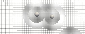
Segment of the computational mesh illustrating the local mesh refinement and the discretization of the particle surfaces. Note that the right particle appears smaller due to its slightly larger distance to the intersecting plane.

The efficient application of the overall method on high-performance computers is enabled by a dynamic load-balancing strategy (Schneiders et al. Reference Schneiders, Grimmen, Meinke and Schröder2015a ). An iterative strong-coupling scheme is used to fully converge the momentum and energy transfer across the fluid–particle interfaces (Schneiders et al. Reference Schneiders, Günther, Meinke and Schröder2016a ). To prevent the particles from interpenetrating, the collision model by Glowinski et al. (Reference Glowinski, Pan, Hesla, Joseph and Périaux2001) is applied. Although more precise collision models have been considered in the literature (Kempe & Fröhlich Reference Kempe and Fröhlich2012), in the present study only dilute flows are considered and collisions are statistically insignificant.

2.5 Flow configuration

A decaying homogeneous isotropic turbulence field is considered. The initial velocity field is isothermal, divergence-free and satisfies the model spectrum $E(\unicode[STIX]{x1D705})=(3u_{0}^{2}/2)(\unicode[STIX]{x1D705}/\unicode[STIX]{x1D705}_{p}^{2})\exp (-\unicode[STIX]{x1D705}/\unicode[STIX]{x1D705}_{p})$ with the root-mean-square (r.m.s.) velocity $u_{0}$ , the peak wavenumber $\unicode[STIX]{x1D705}_{p}=4\unicode[STIX]{x1D705}_{0}$ and the base wavenumber $\unicode[STIX]{x1D705}_{0}=2\unicode[STIX]{x03C0}/L$ . The random velocity fluctuations are computed on a uniform background mesh with $256^{3}$ cells in a cubic domain of edge length $L$ using the technique proposed by Orszag (Reference Orszag1969). The above model spectrum was proposed by Schumann & Patterson (Reference Schumann and Patterson1978) and is appropriate to describe the initial period of decay of grid-generated isotropic turbulence (Nomura & Post Reference Nomura and Post1998). By applying this spectrum, Elghobashi & Truesdell (Reference Elghobashi and Truesdell1992) obtained an energy decay rate similar to the conditions observed in the wind-tunnel measurements by Snyder & Lumley (Reference Snyder and Lumley1971). Several studies of particle-laden decaying turbulence have since been based on this particular model spectrum (Elghobashi & Truesdell Reference Elghobashi and Truesdell1992, Reference Elghobashi and Truesdell1993; Druzhinin Reference Druzhinin2001; Ferrante & Elghobashi Reference Ferrante and Elghobashi2003; Lucci et al. Reference Lucci, Ferrante and Elghobashi2010, Reference Lucci, Ferrante and Elghobashi2011; Strutt, Tullis & Lightstone Reference Strutt, Tullis and Lightstone2011; Gao, Li & Wang Reference Gao, Li and Wang2013; Schneiders, Meinke & Schröder Reference Schneiders, Meinke and Schröder2016b ). This configuration was also considered in Schneiders et al. (Reference Schneiders, Günther, Meinke and Schröder2016a ) to validate the numerical method outlined in § 2.4 for the motion of 6400 large ( $d_{p}>\unicode[STIX]{x1D702}$ ) spherical particles in decaying turbulence against the results of Lucci et al. (Reference Lucci, Ferrante and Elghobashi2010) and Gao et al. (Reference Gao, Li and Wang2013). A very good agreement with the references was observed and the efficiency of the numerical scheme was discussed in detail. The initial pressure field is obtained by solving the Poisson equation in wavenumber space and a subsequent inverse Fourier transform. The reference viscosity is determined to yield an initial Taylor-scale-based Reynolds number of $Re_{\unicode[STIX]{x1D706},0}=\unicode[STIX]{x1D70C}u_{0}\unicode[STIX]{x1D706}/\unicode[STIX]{x1D707}=79.1$ . The turbulent Mach number is set to $M_{t}=u_{0}/a_{\infty }=0.1$ to achieve a large computational time step without compressibility effects. The initial dissipation rate of $\unicode[STIX]{x1D716}_{0}/\unicode[STIX]{x1D716}_{ref}=5.23$ at $t=0$ , non-dimensionalized by $\unicode[STIX]{x1D716}_{ref}=\unicode[STIX]{x1D70C}u_{0}^{3}/L$ , is close to the theoretical value of 5.22 (Gao et al. Reference Gao, Li and Wang2013). Table 1 lists several non-dimensional quantities describing the initial single-phase flow field.

Table 1.

Initial properties of the generated single-phase turbulent flow field: Taylor-scale Reynolds number $Re_{\unicode[STIX]{x1D706}}$ , Prandtl number $Pr$ , turbulent Mach number $M_{t}$ , ratio of peak to base wavenumbers $\unicode[STIX]{x1D705}_{p}/\unicode[STIX]{x1D705}_{0}$ , ratio of initial dissipation rate $\unicode[STIX]{x1D716}_{0}$ to $\unicode[STIX]{x1D716}_{ref}=\unicode[STIX]{x1D70C}u_{0}^{3}/L$ , and ratios of Kolmogorov length $\unicode[STIX]{x1D702}$ and Taylor length $\unicode[STIX]{x1D706}$ to the domain width  $L$ .

Table 2.

Parameters of the five simulations at injection time $t_{i}^{\ast }=0.28$ : number of particles $N_{p}$ , particle-to-fluid density ratio $\unicode[STIX]{x1D70C}_{p}/\unicode[STIX]{x1D70C}$ , ratio of particle diameter $d_{p}$ to the Kolmogorov length scale $\unicode[STIX]{x1D702}$ and domain length  $L$ , and particle volume and mass fractions $\unicode[STIX]{x1D719}_{v}$ and  $\unicode[STIX]{x1D719}_{m}$ .

The particles are released at random positions after the turbulent flow field has sufficiently developed. This sufficiently developed turbulent state is determined by the convergence of the velocity-derivative skewness to approximately $S_{u}=0.44$ at time level $t_{i}$ . This procedure avoids a bias of the particle motion on the initially artificial turbulent field (see Elghobashi & Truesdell Reference Elghobashi and Truesdell1993; Ferrante & Elghobashi Reference Ferrante and Elghobashi2003; Lucci et al. Reference Lucci, Ferrante and Elghobashi2010; Strutt et al. Reference Strutt, Tullis and Lightstone2011). The particle release time is $t_{i}^{\ast }=0.28$ , where the non-dimensional time $t^{\ast }=t\unicode[STIX]{x1D716}_{0}/u_{0}^{2}$ is computed using the initial viscous dissipation rate $\unicode[STIX]{x1D716}_{0}$ obtained from the corresponding single-phase simulations (Gao et al. Reference Gao, Li and Wang2013). At release time, the Reynolds number is approximately $Re_{\unicode[STIX]{x1D706}}(t_{i})=52.9$ . 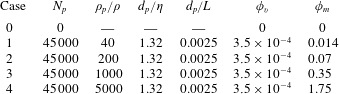The particle velocities are initialized with the local fluid velocity and zero angular velocity. The parameters of the four cases involving $N_{p}=45\,000$ particles are listed in table 2, where a constant particle diameter $d_{p}/L=0.0025$ and constant volume loading of $\unicode[STIX]{x1D719}_{v}=3.5\times 10^{-4}$ are set. 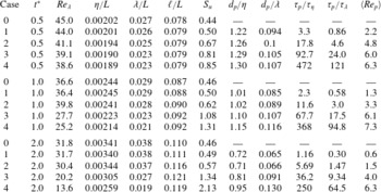By varying the density ratio $\unicode[STIX]{x1D70C}_{p}/\unicode[STIX]{x1D70C}$ , mass loadings from 0.014 to 1.75 and different ratios of particle inertia to fluid inertia are realized. Case 0 represents the particle-free flow field, which serves as a reference for comparison with the particle-laden cases. The temporal development of several non-dimensional numbers involving the characteristic lengths and times of the particle scale ( $d_{p}$ , $\unicode[STIX]{x1D70F}_{p}$ ), the Kolmogorov scale ( $\unicode[STIX]{x1D702}$ , $\unicode[STIX]{x1D70F}_{\unicode[STIX]{x1D702}}$ ), the Taylor scale ( $\unicode[STIX]{x1D706},\unicode[STIX]{x1D70F}_{\unicode[STIX]{x1D706}}$ ) and the integral scale ( $\ell$ , $\unicode[STIX]{x1D70F}_{\ell }$ ) are listed in table 3. It can be seen that $d_{p}\sim \unicode[STIX]{x1D702}$ throughout the simulations and the mean particle Reynolds number ranges from $\langle Re_{p}\rangle \sim 1$ in case 1 to $\langle Re_{p}\rangle \sim 6$ in case 4. The Stokes numbers based on the Kolmogorov and Taylor time scales range from $\unicode[STIX]{x1D70F}_{p}/\unicode[STIX]{x1D70F}_{\unicode[STIX]{x1D702}}\sim 2$ and $\unicode[STIX]{x1D70F}_{p}/\unicode[STIX]{x1D70F}_{\unicode[STIX]{x1D706}}\sim 0.5$ in case 1 to $\unicode[STIX]{x1D70F}_{p}/\unicode[STIX]{x1D70F}_{\unicode[STIX]{x1D702}}\sim 350$ and $\unicode[STIX]{x1D70F}_{p}/\unicode[STIX]{x1D70F}_{\unicode[STIX]{x1D706}}\sim 100$ in case 4. Note that the Kolmogorov length and time scales are computed by $\unicode[STIX]{x1D702}(t)=(\unicode[STIX]{x1D708}^{3}/\langle \unicode[STIX]{x1D716}(t)\rangle )^{1/4}$ and $\unicode[STIX]{x1D70F}_{\unicode[STIX]{x1D702}}(t)=(\unicode[STIX]{x1D708}/\langle \unicode[STIX]{x1D716}(t)\rangle )^{1/2}$ using the mean viscous dissipation rate $\langle \unicode[STIX]{x1D716}\rangle (t)$ at time  $t$ . As will be discussed in the following section, the particles strongly influence the dissipation rate close to their surfaces, such that $\unicode[STIX]{x1D702}$ and $\unicode[STIX]{x1D70F}_{\unicode[STIX]{x1D702}}$ are considered to define the mean viscous microscale of the two-phase system.

Table 3.

Non-dimensional groups of the five simulations and time levels $t^{\ast }=0.5$ , 1 and 2: Taylor-scale Reynolds number $Re_{\unicode[STIX]{x1D706}}$ , ratio of Kolmogorov length $\unicode[STIX]{x1D702}$ , Taylor length $\unicode[STIX]{x1D706}$ and integral length $\ell$ to the domain length $L$ , velocity-derivative skewness $S_{u}$ , ratio of particle diameter $d_{p}$ to $\unicode[STIX]{x1D702}$ and $\unicode[STIX]{x1D706}$ , ratio of particle response time $\unicode[STIX]{x1D70F}_{p}$ to Kolmogorov time scale $\unicode[STIX]{x1D70F}_{\unicode[STIX]{x1D702}}$ and Taylor time scale $\unicode[STIX]{x1D70F}_{\unicode[STIX]{x1D706}}$ , and mean particle Reynolds number $\langle Re_{p}\rangle$ .

Figure 2.

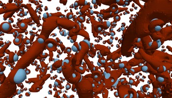
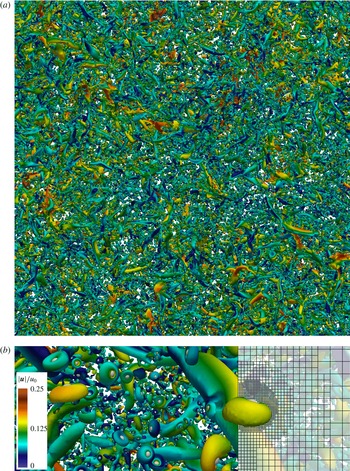
Illustration of the turbulent particle-laden flow field of case 3 at time $t^{\ast }=1$ by $\unicode[STIX]{x1D706}_{2}$ contours, coloured by velocity magnitude: parallel projection of the periodic flow field (a); close-up view revealing the local mesh refinement and vortical structures around individual particles (b).

At injection time $t_{i}^{\ast }$ , the $256^{3}$ mesh is adaptively refined to resolve the particle surfaces and the local flow gradients. The single-phase flow field, computed until time level $t_{i}^{\ast }$ on the background mesh, is prolongated onto the locally refined mesh. Since $\unicode[STIX]{x1D702}(t)\unicode[STIX]{x1D705}_{max}>1$ (Eswaran & Pope Reference Eswaran and Pope1988) holds for the single-phase flow, where $\unicode[STIX]{x1D705}_{max}$ is the maximum resolvable wavenumber on the background mesh, the basic grid resolution is sufficient to be considered a direct numerical simulation. Upon injection of the particles, the additional velocity gradients induced by the presence of the particles are captured by the locally refined mesh. Since all relevant scales are resolved in these computations, we denote them as direct particle–fluid simulations (DPFS). The locally refined mesh around each particle has a minimum spacing of $\unicode[STIX]{x0394}x\approx d_{p}/10$ (see figure 1). Using this mesh spacing, a sufficient resolution of the flow around each particle is obtained and a large number of particles can be simulated to achieve significant particle statistics and mass loadings with turbulence modulation effects. Note that the present cut-cell method provides a convincing accuracy even at relatively low mesh resolution due to the sharp resolution of the embedded boundaries, which is in contrast to classical immersed-boundary methods (Schneiders et al. Reference Schneiders, Günther, Meinke and Schröder2016a ). Since the particle diameter is considered constant and typical particle Reynolds numbers are $Re_{p}=O(5)$ (see table 3), i.e. the particle wakes are predominantly steady, the spatial resolution requirements are roughly constant at all times. That is, the computational mesh is adaptively refined to resolve the particle boundary layers in regular, spherical patterns (see figure 1). For the sake of computational efficiency, the vortical structures of the bulk flow are not further locally refined, although this is possible in principle. Each of the dynamic meshes in the particle-resolved simulations (cases 1–4) contains approximately $2\times 10^{9}$ cells on average, i.e. roughly 120 times more cells than for the direct numerical simulation of the corresponding single-phase flow. The simulations were performed on 48 000 compute cores. Figure 2 shows the instantaneous vortical structures for case 3 at time level $t^{\ast }=1$ determined by contours of the $\unicode[STIX]{x1D706}_{2}$ -criterion (Jeong & Hussain Reference Jeong and Hussain1995). The symmetrical vortical structures forming around the particles are evidenced by the close-up view in figure 2.

3.1 Turbulent kinetic energy budget

In particle-laden decaying isotropic turbulence, the temporal change of total fluid kinetic energy $E_{k}=\int _{\unicode[STIX]{x1D6F6}_{f}}e_{k}\,\text{d}V$ , where $e_{k}=\unicode[STIX]{x1D70C}\boldsymbol{u}^{2}/2$ , is determined by the balance of total interphase kinetic energy transfer $\unicode[STIX]{x1D6F9}$ and the integrated dissipation rate ${\mathcal{E}}$ in the fluid domain  $\unicode[STIX]{x1D6F6}_{f}$ , i.e.

The integral rate of dissipation equals

with the inner tensor product $\unicode[STIX]{x1D63C}\boldsymbol{ : }\unicode[STIX]{x1D63D}=\unicode[STIX]{x1D608}_{ij}\unicode[STIX]{x1D609}_{ji}$ and the pressure dilatation $(\unicode[STIX]{x1D735}\boldsymbol{\cdot }\boldsymbol{u})p$ (see appendix A). Since the flow field considered is nearly incompressible, the divergence $\unicode[STIX]{x1D735}\boldsymbol{\cdot }\boldsymbol{u}$ is small and the dissipation rate can be approximated by

which is a positive quantity and thus acts as a sink to the fluid kinetic energy balance. On the contrary, $\unicode[STIX]{x1D6F9}$ can act as source or sink (Ferrante & Elghobashi Reference Ferrante and Elghobashi2003) depending on the acceleration of the particles. The interphase exchange term is determined by the rate of kinetic energy given by (2.8), transferred from individual particles to the fluid, i.e.

The quantity $\unicode[STIX]{x1D6F9}$ represents the direct transfer of kinetic energy between the two phases via surface forces. In addition, the particles also indirectly influence the kinetic energy $E_{k}$ by manipulating the rate of dissipation  ${\mathcal{E}}$ , i.e. via volume forces given in (3.2). Accordingly, the kinetic energy of an individual particle, $k=(m\boldsymbol{v}^{2}+\widetilde{\unicode[STIX]{x1D74E}}\boldsymbol{\cdot }(\widetilde{\boldsymbol{{\mathcal{I}}}}\widetilde{\unicode[STIX]{x1D74E}}))/2$ , changes by $\text{d}k_{p}/\text{d}t=-\unicode[STIX]{x1D713}_{p}(t)$ , such that the global kinetic energy of the particles, $K=\sum _{p=1}^{N_{p}}k_{p}$ , evolves as

Figure 3.

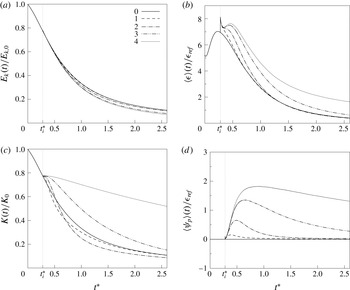
Temporal variation of the global kinetic energy budget: (a) total fluid kinetic energy $E_{k}$ normalized by its initial value; (b) mean viscous dissipation rate $\langle \unicode[STIX]{x1D716}\rangle$ normalized by $\unicode[STIX]{x1D716}_{ref}=\unicode[STIX]{x1D70C}u_{0}^{3}/L$ ; (c) total particle kinetic energy $K$ normalized by $K_{0}=\unicode[STIX]{x1D719}_{m}E_{0}$ (as a reference, $E$ of case 0 is also shown); and (d) mean interphase energy exchange $\langle \unicode[STIX]{x1D713}\rangle$ normalized by $\unicode[STIX]{x1D716}_{ref}$ .

In figure 3, the variations of the individual terms contributing to (3.1) and (3.5) are depicted as a function of time for cases 1–4 in comparison to the single-phase flow case 0. Figure 3(a) shows the temporal development of the fluid kinetic energy. Upon injection of the particles at time $t_{i}^{\ast }=0.28$ , the decay rate of kinetic energy is increased for the particle-laden cases. However, only a minor effect is observed for case 1 due to the small mass loading. At time level $t^{\ast }=1.5$ , the level of kinetic energy is reduced by 0.5 %, 6.5 %, 18 % and 22 % for cases 1–4 relative to case 0. Interestingly, the decay rates in the latter two cases are quite similar, despite the substantial difference in mass loading by a factor of 5. Moreover, the overall reduction appears small compared to previous results published for small particles (30 % reduction for $d_{p}/\unicode[STIX]{x1D702}\sim 0.3$ ) at a similar mass loading and flow configuration by Ferrante & Elghobashi (Reference Ferrante and Elghobashi2003). A first explanation is obtained from an analysis of the mean viscous dissipation rate $\langle \unicode[STIX]{x1D716}\rangle ={\mathcal{E}}/|\unicode[STIX]{x1D6F6}_{f}|$ (figure 3 b) and the mean rate of kinetic energy exchange $\langle \unicode[STIX]{x1D713}\rangle =\unicode[STIX]{x1D6F9}/|\unicode[STIX]{x1D6F6}_{f}|$ (figure 3 d). Both are normalized by the reference dissipation rate $\unicode[STIX]{x1D716}_{ref}=\unicode[STIX]{x1D70C}u_{0}^{3}/L$ . At injection time, a sharp peak of the dissipation rate is observed in the particle-laden cases, which is explained by the instantaneous build-up of the velocity gradients in the particle boundary layers in response to the no-slip condition. Owing to the sharp resolution of the particle surfaces by the present method, mass conservation is satisfied upon the first step after adding the particles. The initial peak is identical in the four particle-laden cases since the total particle surface areas and the initial particle velocities are equal, which leads to initially equal surface stresses. At approximately $t^{\ast }=0.3$ , inertia effects become dominant and the dissipation-rate curves begin to separate. Whereas the dissipation rate in cases 1 and 2, i.e. at relatively small mass loading, relaxes towards the single-phase flow solution rather quickly ( $t^{\ast }=0.7$ and $t^{\ast }=1.3$ ), a strong amplification of the dissipation rate is observed at increasing mass loading, i.e. especially for case 4. At time level $t^{\ast }=1$ , the increase in the dissipation rate over case 0 is 44 % and 70 % in cases 3 and 4. By time level $t^{\ast }=2$ , the dissipation rate in case 4 is still approximately three times higher than in the no-particle case despite a large portion of the initial fluid kinetic energy having been converted (figure 3 a). This strong increase of $\langle \unicode[STIX]{x1D716}\rangle$ is a consequence of the high particle inertia leading to strong velocity gradients in the particle boundary layers and thus a local increase of the dissipation rate.

In spite of the strong increase of the dissipation rate with increasing $\unicode[STIX]{x1D70C}_{p}/\unicode[STIX]{x1D70C}$ evidenced in figure 3(b), the decay rates of cases 3 and 4 (figure 3 a) show a comparable temporal development. This is explained by the additional direct transfer of kinetic energy between the phases via surface forces. The energy transfer rate towards the fluid, $\langle \unicode[STIX]{x1D713}\rangle$ , is positive for cases 1–4 at each time level, as shown in figure 3(d). Thus, the direct transfer of kinetic energy via surface forces acts as a source to the fluid kinetic energy balance in the present cases. Apparently, the indirect reduction of fluid kinetic energy by the additional viscous dissipation induced by the particles is partially compensated by $\langle \unicode[STIX]{x1D713}\rangle$ . The interaction between these two effects explains the moderate decrease of kinetic energy compared to the particle-free case (figure 3 a).

Since $\unicode[STIX]{x1D6F9}(t)>0$ , the total kinetic energy of the particles decreases with time (see figure 3 c). Owing to the small particle inertia in case 1, the particles quickly lose energy at a rate much higher than the fluid kinetic energy decay rate. As seen in figure 3(d), in this case the coupling rate beyond time level $t^{\ast }=0.5$ quickly approaches zero such that the decay rate of $K$ is damped. The fluid and particle phase kinetic energies eventually reach an equilibrium at $t^{\ast }=2$ . For case 2, the higher particle inertia leads to an extended transfer of kinetic energy to the fluid (figure 3 d) such that the relative particle kinetic energy decreases below that of case 1 and the fluid kinetic energy of case 0. Similarly as for case 1, the particle energy asymptotically approaches the fluid energy curve, but significantly slower. A similar trend is observed in cases 3 and 4, where the increasing particle inertia leads to a much slower decay of the relative particle energy, which does not fall below the fluid kinetic energy for the time span covered by the present simulations.

Figure 4.

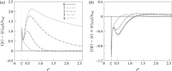
Effective decay rates due to the presence of the particles compared to case 0: (a) particle-induced dissipation rate $\langle \unicode[STIX]{x1D716}\rangle -\langle \unicode[STIX]{x1D716}\rangle _{C0}$ ; and (b) particle-induced decay rate $\langle \unicode[STIX]{x1D713}\rangle -\langle \unicode[STIX]{x1D716}\rangle +\langle \unicode[STIX]{x1D716}\rangle _{C0}$ .

The results for the mean dissipation and coupling rates are in qualitatively good agreement with the results for larger particles ( $d_{p}/\unicode[STIX]{x1D702}\sim 16$ ) by Lucci et al. (Reference Lucci, Ferrante and Elghobashi2010). At a similar range of particle Stokes numbers, they observed a significant increase of $\langle \unicode[STIX]{x1D716}\rangle$ and $\langle \unicode[STIX]{x1D713}\rangle$ for increasing $\unicode[STIX]{x1D70C}_{p}/\unicode[STIX]{x1D70C}$ , but at much smaller $\unicode[STIX]{x1D70C}_{p}/\unicode[STIX]{x1D70C}$ and larger $d_{p}$ . Moreover, the dissipation rate was shown to remain above the dissipation rate of the corresponding single-phase flow, which matches the variation of $\langle \unicode[STIX]{x1D716}\rangle$ in cases 3 and 4 shown in figure 4(b). To estimate the particle-induced portion of the global dissipation rate, figure 4(a) shows the difference between $\langle \unicode[STIX]{x1D716}\rangle$ in the four particle-laden cases and in case 0, i.e. $\langle \unicode[STIX]{x1D716}\rangle -\langle \unicode[STIX]{x1D716}\rangle _{C0}$ , as a function of time. As already observed in figure 4(b), the dissipation rate in case 1 quickly relaxes towards the particle-free solution. With increasing particle inertia, the particle-induced dissipation becomes significantly stronger and reaches its peak once the particles have fully adapted to the ambient fluid motion. Subsequently, the particle-induced dissipation rate decays regularly, corresponding to the decaying particle kinetic energy shown in figure 3(c). Likewise, the decay rate of $\langle \unicode[STIX]{x1D716}\rangle -\langle \unicode[STIX]{x1D716}\rangle _{C0}$ reduces with increasing particle mass. In the weak-inertia cases 1 and 2 the dissipation rate eventually falls below its single-phase counterpart, which is partially explained by the amplified decay of fluid kinetic energy at early time levels. The effective rate of change of $E_{k}$ due to the presence of the particles, approximated by $\langle \unicode[STIX]{x1D713}\rangle -\langle \unicode[STIX]{x1D716}\rangle +\langle \unicode[STIX]{x1D716}\rangle _{C0}$ , is shown in figure 4(b). In the initial phase after addition of the particles, the particle-induced dissipation dominates the release of momentum by the particles. The balance between $\langle \unicode[STIX]{x1D713}\rangle$ and $\langle \unicode[STIX]{x1D716}\rangle -\langle \unicode[STIX]{x1D716}\rangle _{C0}$ then gradually shifts towards positive values, i.e. an effective energy entry in the fluid phase. The time level at which the positive balance is attained increases from $t^{\ast }=0.62$ in case 1, to $t^{\ast }=0.91$ in case 2, and $t^{\ast }=1.19$ cases 3 and 4. At this time, the additional dissipation due to the particle motion is compensated by their release of kinetic energy via $\unicode[STIX]{x1D713}$ . Note that the effective decay rate in cases 3 and 4 behaves very similarly. This leads to the variation of $E_{k}$ observed in figure 3(a), despite the strong differences in $\langle \unicode[STIX]{x1D716}\rangle$ (figure 3 b) and $\langle \unicode[STIX]{x1D713}\rangle$ (figure 3 d) between the two cases.

Compared to studies previously published for smaller particles, fundamental differences are observed with respect to the decay rate of fluid kinetic energy. Numerical studies on small particles in turbulence are typically conducted using point-particle models, which do not resolve the velocity field disturbances in the vicinity of the particles. Ferrante & Elghobashi (Reference Ferrante and Elghobashi2003) investigate, among other cases, particles at $d_{p}/\unicode[STIX]{x1D702}\sim 0.3$ , where the density ratio $\unicode[STIX]{x1D70C}_{p}/\unicode[STIX]{x1D70C}=1000$ and the mass loading $\unicode[STIX]{x1D719}_{m}=1$ are similar to the present case 3. They report a negative coupling rate $\langle \unicode[STIX]{x1D713}\rangle$ , i.e. an energy transfer from the fluid to the particles and a dissipation rate lower than that of the particle-free case, both of which are in clear contrast to the present results. At this point it is not clear whether this is an effect of the different particle diameters and therefore different particle Stokes numbers or caused by the deficiencies of the point-particle approach, which is strictly only valid at $d_{p}\ll \unicode[STIX]{x1D702}$ . The results in Schneiders et al. (Reference Schneiders, Meinke and Schröder2016b ) for $d_{p}\sim \unicode[STIX]{x1D702}$ indicate that point-particle models vastly underestimate the viscous dissipation rate when $d_{p}\ll \unicode[STIX]{x1D702}$ is not fulfilled. Moreover, in point-particle models the coupling rate $\unicode[STIX]{x1D713}$ usually originates from point forces. Its formulation is therefore different compared to the present formulation (2.8), since in the present study the particle surfaces are explicitly resolved. These different formulations will be discussed in § 3.4.

3.2 Spectral distribution of energy

The above analysis of the kinetic energy decay rates illustrates the overall distribution and exchange of energy between the phases. However, the time and length scales associated with this interaction are not apparent. To gain a clearer explanation of the mechanisms behind the behaviour observed in figure 3, we analyse the spectral distribution of fluid kinetic energy as well as the spectral energy transfer and decay rates.

The wavenumber space equivalent of (3.1) is obtained by a Fourier transform of the momentum equation in (2.1b ), which leads to (Ferrante & Elghobashi Reference Ferrante and Elghobashi2003)

where $\widehat{E}(\unicode[STIX]{x1D73F})=\widehat{\boldsymbol{u}}(\unicode[STIX]{x1D73F})\boldsymbol{\cdot }\widehat{\boldsymbol{u}}(\unicode[STIX]{x1D73F})/2$ is the kinetic energy at wavenumber $\unicode[STIX]{x1D73F}$ determined by the Fourier-transformed velocity vector $\widehat{\boldsymbol{u}}(\unicode[STIX]{x1D73F})$ . The spectral interphase exchange term

where $\text{Re}\{\cdot \}$ denotes the real part, is computed using the local forces at segments of the particle surfaces $\unicode[STIX]{x1D6E4}$ , i.e. $\boldsymbol{f}=(p\boldsymbol{n}-\unicode[STIX]{x1D749}\boldsymbol{\cdot }\boldsymbol{n})A_{\unicode[STIX]{x1D6E4}}/V$ . The spectral dissipation rate is

The transfer rate $\widehat{T}(\unicode[STIX]{x1D705})$ stems from the transformed nonlinear convective terms in (2.1b ) and represents local and non-local interactions between all triads of wavelengths $\unicode[STIX]{x1D73F}$ , $\unicode[STIX]{x1D73F}^{\prime }$ and $\unicode[STIX]{x1D73F}^{\prime \prime }$ , i.e. forming a triangle ( $\unicode[STIX]{x1D73F}^{\prime \prime }=\unicode[STIX]{x1D73F}-\unicode[STIX]{x1D73F}^{\prime }$ ) in wavenumber space (Domaradzki & Rogallo Reference Domaradzki and Rogallo1990),

which is written using Einstein notation, $\text{Im}\{\cdot \}$ denotes the imaginary part and $\unicode[STIX]{x1D6FF}_{jk}$ the Kronecker delta. To compute the energy spectrum, the velocity field is reduced from the locally refined mesh to the uniform $256^{3}$ background mesh using a sharp spectral filter. The cut-off wavenumber is set to the maximum resolvable wavenumber of the background mesh, $\unicode[STIX]{x1D705}_{c}=\unicode[STIX]{x1D705}_{max}$ , such that the filtering process preserves the energy spectrum at wavenumbers below $\unicode[STIX]{x1D705}_{max}$ . Subsequently, the energy spectrum is computed via a fast Fourier transform of the filtered velocity field. Since the background mesh resolves scales approximately down to the Kolmogorov length scale, the overall level of kinetic energy is mostly preserved by this conversion while the computational effort is reduced considerably. The energy spectrum beyond $\unicode[STIX]{x1D705}_{max}$ , i.e. at the particle scale, is not recovered by this procedure although it is resolved by the numerical scheme. However, at this scale the flow field is mainly dominated by the locally laminar flow around the particles such that significant additional turbulent fluctuations in the bulk flow are not expected. The spectral transfer rate is computed directly from (3.9) in parallel on $O(10\,000)$ compute cores. Finally, the various three-dimensional spectral quantities are converted to one-dimensional spectra by averaging over spherical shells. The one-dimensional energy flux from wavenumber $\unicode[STIX]{x1D705}$ to all higher wavenumbers (Elghobashi & Truesdell Reference Elghobashi and Truesdell1993) follows as

Figure 5.

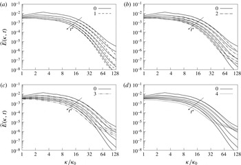
Evolution of the fluid kinetic energy spectra $\widehat{E}(\unicode[STIX]{x1D705},t)$ with time; comparison of the particle-laden results (cases 1–4 in (a–d) respectively) with the particle-free case 0 at five consecutive time levels between $t^{\ast }=0.5$ and $t^{\ast }=2.5$ for $\unicode[STIX]{x0394}t^{\ast }=0.5$ .

Figure 6.

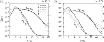
Direct comparison of the fluid kinetic energy spectra of the individual cases at time levels $t^{\ast }=1$  (a) and 2 (b) (shown as log–log and log–linear plots).

In figure 5 the spectra of fluid kinetic energy computed for the particle-laden cases are compared to the single-phase flow results at five consecutive time levels between $t^{\ast }=0.5$ and $t^{\ast }=2.5$ . It is seen that at early time levels the particles lead to an enhanced energy decay at higher wavenumbers. Fluid kinetic energy is absorbed from the intermediate wavenumber range and the dissipation at high wavenumbers is reduced. For case 1 involving weakly inertial particles, this behaviour is seen to persist up to the final time level. At increasing particle inertia, the initial trend is reverted at later times after the energy cascade has adapted to the disturbances invoked by the particles. It can be seen that in cases 3 and 4 the energy decay rate at low and intermediate wavenumbers and the level of dissipation at high wavenumbers are significantly increased. For case 4, almost a steady spectrum is observed in the high wavenumber range $\unicode[STIX]{x1D705}/\unicode[STIX]{x1D705}_{0}>80$ , which suggests that the energy content in this part of the spectrum is dominated by the inertial particle dynamics. Clearly, the manipulation of the fluid energy spectra covers a broader range of wavenumbers at increasing $\unicode[STIX]{x1D70C}_{p}/\unicode[STIX]{x1D70C}$ , where for case 4 the whole spectrum is biased at $t^{\ast }>1$ . It may be presumed that beyond the maximum shown wavenumber $\unicode[STIX]{x1D705}_{max}$ , i.e. at the particle scale, the energy spectrum of the weak-inertia case 1 approximately follows the single-phase spectrum. For cases 3 and 4, however, the additional kinetic energy induced by the particle acceleration leads to extended tails of the energy spectrum. The direct comparison of the different spectra at time levels $t^{\ast }=1$ and $t^{\ast }=2$ in figure 6 illustrates the effect of increasing particle inertia. The particles in case 2 receive energy from the wavenumber range $4<\unicode[STIX]{x1D705}/\unicode[STIX]{x1D705}_{0}$ while case 1 barely modulates the spectrum. For cases 3 and 4 a strong reduction of the energy content at the lowest wavenumbers is observed at $t^{\ast }=2$ in reaction to the momentum exchange between the phases and the strong increase of dissipation at large $\unicode[STIX]{x1D705}$ . The wavenumber at which the particle-free spectrum is crossed decreases at increasing $\unicode[STIX]{x1D70C}_{p}/\unicode[STIX]{x1D70C}$ . The results are in agreement with the experimental results on large ( $d_{p}/\unicode[STIX]{x1D702}\sim 5$ ) inertial particles in turbulence by Calabrese & Middleman (Reference Calabrese and Middleman1979). They state that energy is removed at low wavenumbers while the energy-containing range is extended towards larger wavenumbers.

Figure 7.

Comparison of the spectral kinetic energy budgets of cases 0–4 at time level $t^{\ast }=1$ : (a) decay rate $\unicode[STIX]{x2202}\widehat{E}(\unicode[STIX]{x1D705})/\unicode[STIX]{x2202}t$ ; (b) spectral transfer rate $\widehat{T}(\unicode[STIX]{x1D705})$ ; (c) viscous dissipation rate $\widehat{{\mathcal{E}}}(\unicode[STIX]{x1D705})$ ; and (d) interphase exchange rate $\widehat{\unicode[STIX]{x1D6F9}}(\unicode[STIX]{x1D705})$ .

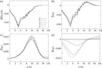
The evolution of the energy spectra is elucidated by a breakdown of (3.6) shown in figure 7 for time level $t^{\ast }=1$ . It is seen from the decay rate $-\unicode[STIX]{x2202}\widehat{E}(\unicode[STIX]{x1D705})/\unicode[STIX]{x2202}t$ that the particles consume fluid kinetic energy mainly from the range $\unicode[STIX]{x1D705}/\unicode[STIX]{x1D705}_{0}<16$ (figure 7 a). The decay rate is amplified at the lowest wavenumbers when $\unicode[STIX]{x1D70C}_{p}/\unicode[STIX]{x1D70C}$ is increased such that for cases 3 and 4 a significant contribution to the particle kinetic energy comes from the largest scales of the flow. The absolute value of the energy transfer function $T(\unicode[STIX]{x1D705})$ of the particle cases shown in figure 7(b) is smaller over the whole spectrum and the damping of the spectral transfer becomes stronger at increasing particle inertia. This behaviour was also observed for smaller particles ( $d_{p}/\unicode[STIX]{x1D702}\sim 0.3$ ) by Ferrante & Elghobashi (Reference Ferrante and Elghobashi2003). In contrast to their results, the wavenumber that separates the sending and receiving range of the spectrum ( $\unicode[STIX]{x1D705}/\unicode[STIX]{x1D705}_{0}=12$ ), i.e. at which $\widehat{T}(\unicode[STIX]{x1D705})=0$ , is hardly altered by the particles. The variation of $\widehat{T}(\unicode[STIX]{x1D705})$ proves the increased decay rates for the particulate cases to be primarily the result of dissipation and interphase energy exchange. The particles reduce the dissipation rate (figure 7 c) in the intermediate wavenumber range, which again is in agreement with Ferrante & Elghobashi (Reference Ferrante and Elghobashi2003). Therefore, the strong increase of the dissipation rate evidenced in figure 3(b) for cases 3 and 4 is the result of a strong increase of $\widehat{{\mathcal{E}}}(\unicode[STIX]{x1D705})$ at larger wavenumbers ( $\unicode[STIX]{x1D705}/\unicode[STIX]{x1D705}_{0}>80$ ), i.e. the particles reduce the dissipation rate of the background flow and locally induce a strong level of dissipation. The spectral interphase exchange (figure 7 d) underlines that the energy removal by the particles moves to lower $\unicode[STIX]{x1D705}$ and is amplified when particle inertia increases. At wavenumbers $\unicode[STIX]{x1D705}/\unicode[STIX]{x1D705}_{0}>30$ , the particles release kinetic energy to the fluid by accelerating the flow close to their surfaces. At the highest wavenumbers, the variation of $\widehat{{\mathcal{E}}}(\unicode[STIX]{x1D705})$ and $\widehat{\unicode[STIX]{x1D6F9}}(\unicode[STIX]{x1D705})$ is almost constant in case 2 and even slightly increasing for cases 3 and 4. This indicates that an additional contribution to the overall level of dissipation and the interphase exchange of energy comes from scales smaller than the particle diameter and thus smaller than the Kolmogorov scale.

Figure 8.

Comparison of the spectral kinetic energy budgets of cases 0–4 at time level $t^{\ast }=1$ : (a) effective decay rate $\widehat{\unicode[STIX]{x1D6F9}}(\unicode[STIX]{x1D705})-\widehat{{\mathcal{E}}}(\unicode[STIX]{x1D705})$ ; and (b) spectral flux $\widehat{F}(\unicode[STIX]{x1D705})$ .

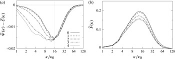
The qualitative behaviour of the spectra seen in figure 7 is very similar among the different particle-laden cases. Moreover, the crossover wavenumbers separating regions of energy gain or loss appear to be universal. We infer that the basic small-scale flow topology is similar in the studied cases and therefore mainly determined by the length-scale ratio $d_{p}/\unicode[STIX]{x1D702}$ , which is constant. On the other hand, the strength of the decay rates and the width of the wavenumber range involved in the energy conversion process are determined by the ratio of particle relaxation time $\unicode[STIX]{x1D70F}_{p}$ to the characteristic fluid time scales that describe the ratio of particle to fluid inertia. This leads to a clear distinction of two sectors, which are illustrated by the balance $\widehat{\unicode[STIX]{x1D6F9}}(\unicode[STIX]{x1D705})-\widehat{{\mathcal{E}}}(\unicode[STIX]{x1D705})$ shown in figure 8(a). The increased decay rates of fluid kinetic energy seen in figure 7(a) manifest at low wavenumbers ( $\unicode[STIX]{x1D705}/\unicode[STIX]{x1D705}_{0}<16$ ), where also the main differences in the spectral decay rates among the individual cases are observed. At higher wavenumbers ( $\unicode[STIX]{x1D705}/\unicode[STIX]{x1D705}_{0}>16$ ), the decay rates compared to the particle-free case are damped, which is the result of a reduction of $\widehat{{\mathcal{E}}}(\unicode[STIX]{x1D705})$ in the intermediate wavenumber region and a turn to positive $\widehat{\unicode[STIX]{x1D6F9}}(\unicode[STIX]{x1D705})$ in the high wavenumber range. Interestingly, figure 8(a) shows that the energy released to the fluid at $\unicode[STIX]{x1D705}/\unicode[STIX]{x1D705}_{0}>100$ is immediately dissipated, i.e. $\widehat{\unicode[STIX]{x1D6F9}}(\unicode[STIX]{x1D705})-\widehat{{\mathcal{E}}}(\unicode[STIX]{x1D705})\approx 0$ at $\unicode[STIX]{x1D705}/\unicode[STIX]{x1D705}_{0}>100$ . At the same time, the net flux of kinetic energy from each wavenumber $\unicode[STIX]{x1D705}$ to the higher wavenumbers (figure 8 b) is damped over the whole spectrum. Compared to the particle-free flow, the contribution of $\widehat{F}(\unicode[STIX]{x1D705})$ to the high wavenumber energy level is reduced. However, since the overall decay rate $\unicode[STIX]{x2202}\widehat{E}(\unicode[STIX]{x1D705})/\unicode[STIX]{x2202}t$ does not vary significantly at the highest wavenumbers among the different cases (figure 7 a), we assume that the release of energy via $\widehat{\unicode[STIX]{x1D6F9}}(\unicode[STIX]{x1D705})$ substitutes the retrieval of energy via $\widehat{T}(\unicode[STIX]{x1D705})$ in the spectral balance of kinetic energy. That is, the acceleration of the fluid elements surrounding the particles suppresses the spectral transfer of energy to the smallest scales.

3.3 Near-particle-surface flow pattern

The spectral analysis shows that the particles insert energy at intermediate to high wavenumbers via the forces acting at the particle surfaces. The energy entry is offset by the strong increase of viscous dissipation at the highest wavenumbers. We proceed to quantify the typical flow pattern around each particle to understand how the presence of the particles leads to augmentation of energy and local increase of the viscous dissipation rate at high wavenumbers.

Since the viscous dissipation rate (3.3) equals the squared Frobenius norm of the strain-rate tensor, it can be expressed via the eigenvalues of $\unicode[STIX]{x1D64E}$ , i.e.

Letting the eigenvalues be ordered as $\unicode[STIX]{x1D6FC}\geqslant \unicode[STIX]{x1D6FD}\geqslant \unicode[STIX]{x1D6FE}$ , the corresponding eigendirections represent the principal axes of strain, with $\boldsymbol{e}_{\unicode[STIX]{x1D6FC}}$ being the direction of maximum extension rate, $\boldsymbol{e}_{\unicode[STIX]{x1D6FE}}$ the direction of maximum compression rate and $\boldsymbol{e}_{\unicode[STIX]{x1D6FD}}$ an intermediate direction, typically with a bias towards extension.

Table 4.

Statistical quantities of the velocity gradients at time level $t^{\ast }=1$ : average and r.m.s. values of the strain-rate eigenvalues $\unicode[STIX]{x1D6FC}$ , $\unicode[STIX]{x1D6FD}$ and $\unicode[STIX]{x1D6FE}$ , enstrophy generation $\unicode[STIX]{x1D70E}=\unicode[STIX]{x1D74E}\boldsymbol{\cdot }\unicode[STIX]{x1D64E}\unicode[STIX]{x1D74E}$ , and vortex stretching rate $\unicode[STIX]{x1D70E}/\unicode[STIX]{x1D74E}^{2}$ , all of which have been non-dimensionalized by powers of $\langle \unicode[STIX]{x1D74E}^{2}\rangle _{C0}$ computed for case 0.

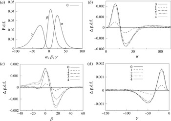
Table 4 shows that the average values $\langle \unicode[STIX]{x1D6FC}\rangle$ and $\langle \unicode[STIX]{x1D6FE}\rangle$ significantly increase with particle inertia, which is expected from the overall higher level of viscous dissipation observed in figure 3(b). The effect of the particles on the strain-rate distribution is demonstrated by the probability density functions (p.d.f.s) of $\unicode[STIX]{x1D6FC}$ , $\unicode[STIX]{x1D6FD}$ and $\unicode[STIX]{x1D6FE}$ given in figure 9. The single-phase solution (figure 9 a) shows the typical pattern observed in other turbulent flows (Diamessis & Nomura Reference Diamessis and Nomura2000), i.e. $\unicode[STIX]{x1D6FC}>0$ and $\unicode[STIX]{x1D6FE}<0$ , which is stipulated by incompressibility ( $\unicode[STIX]{x1D6FC}+\unicode[STIX]{x1D6FD}+\unicode[STIX]{x1D6FE}=0$ ) and $\unicode[STIX]{x1D6FD}$ being more probable at positive values. Figure 9(b–d) shows the difference of the p.d.f.s between the particle-laden cases and the single-phase flow, i.e. $\unicode[STIX]{x0394}\text{p.d.f.}=\text{p.d.f.}|_{i}-\text{p.d.f.}|_{0}$ , $i=1,\ldots ,4$ . It can be seen that with increasing particle inertia the peak of the p.d.f.s is slightly shifted towards zero for all three eigenvalues. However, at the tails of the p.d.f.s of $\unicode[STIX]{x1D6FC}$ and $\unicode[STIX]{x1D6FE}$ , a significant increase is observed. This suggests that the presence of the heavy particles induces local events of high strain rate, which are responsible for the overall higher level of dissipation. Note that the probability densities at higher values of the eigenvalues increasingly contribute to the mean value. This is corroborated by the strong increase of the r.m.s. values $\unicode[STIX]{x1D6FC}^{\prime }$ , $\unicode[STIX]{x1D6FD}^{\prime }$ and $\unicode[STIX]{x1D6FE}^{\prime }$ by roughly 30–40 % in table 4. On the other hand, the increased probability at lower absolute values of the eigenvalues indicates that the background strain rate is attenuated with increasing particle inertia. This behaviour matches the reduction of the spectral dissipation rate at intermediate wavenumbers and strong increase at high wavenumbers discussed above.

Figure 9.

Probability density functions of the strain-rate tensor eigenvalues $\unicode[STIX]{x1D6FC}$ , $\unicode[STIX]{x1D6FD}$ and $\unicode[STIX]{x1D6FE}$ , normalized by $u_{0}/L$ , at time level $t^{\ast }=1$ : (a) p.d.f.s of the particle-free case 0; (b–d) p.d.f. differences $\unicode[STIX]{x0394}\text{p.d.f.}=\text{p.d.f.}|_{i}-\text{p.d.f.}|_{0}$ of particle-laden case  $i$ to the single-phase case 0.

The increase at the tails of the strain-rate eigenvalue distribution was also observed for larger particles ( $d_{p}>\unicode[STIX]{x1D702}$ ) by Lucci et al. (Reference Lucci, Ferrante and Elghobashi2010). However, they reported a slightly increasing level of background dissipation due to the particles in their study. The shift of the p.d.f. peak towards zero was observed for smaller particles ( $d_{p}/\unicode[STIX]{x1D702}\sim 0.3$ ) by Ferrante & Elghobashi (Reference Ferrante and Elghobashi2003). Note that the strong increase of the dissipation rate by high-strain-rate events at the particle surfaces is not resolved by their point-particle model.

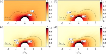
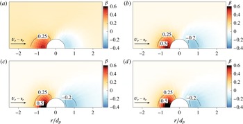
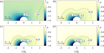
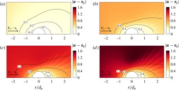
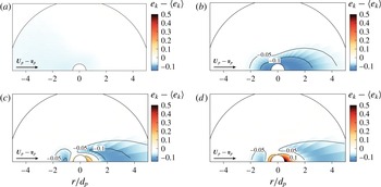
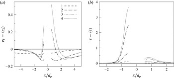
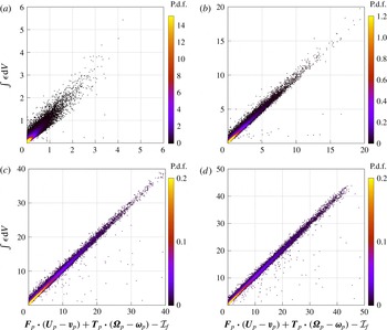
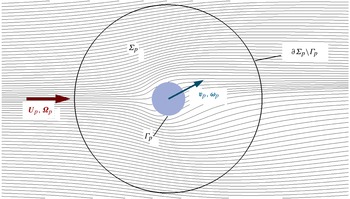
The origin of the high-strain-rate events induced by the particles is illustrated by the mean flow pattern about each particle. In figures 10–12 the average distributions of $\unicode[STIX]{x1D6FC}$ , $\unicode[STIX]{x1D6FD}$ and $\unicode[STIX]{x1D6FE}$ at time level $t^{\ast }=1$ are shown, where the eigenvalues have been normalized by $|\boldsymbol{v}_{p}|/d_{p}$ . For the range of particle Reynolds numbers observed in the present study, the flow field about the particles is axisymmetric. Therefore, the statistics have been determined in polar coordinates in terms of the angle to the relative velocity vector $\boldsymbol{U}_{p}-\boldsymbol{v}_{p}$ and the radial distance to the particle centroids, where $\boldsymbol{U}_{p}$ denotes the velocity of the undisturbed flow about the particle. Note that the quantity $\boldsymbol{U}_{p}$ is not directly accessible in particle-resolved simulations. For each particle we evaluate

where $\unicode[STIX]{x1D6FF}_{p}$ is the local distance to the particle surface $\unicode[STIX]{x1D6E4}_{p}$ and $\unicode[STIX]{x1D6F4}_{p}=\{\boldsymbol{x}\mid 0\leqslant \unicode[STIX]{x1D6FF}_{p}(\boldsymbol{x})/d_{p}\leqslant 6\}$ . In preceding simulations for the laminar flow about a single fixed sphere at the same mesh resolution, we have verified that this procedure recovers the undisturbed flow velocity within 8 % error.

Figure 10.

Mean strain-rate distribution around the particles in a frame aligned with $\boldsymbol{U}_{p}-\boldsymbol{v}_{p}$ for cases 1–4 (a–d, respectively) at time $t^{\ast }=1$ : contours of the largest strain-rate eigenvalue $\unicode[STIX]{x1D6FC}$ normalized by $|\boldsymbol{v}_{p}|/d_{p}$ .

Figure 11.

Mean strain-rate distribution around the particles in a frame aligned with $\boldsymbol{U}_{p}-\boldsymbol{v}_{p}$ for cases 1–4 (a–d, respectively) at time $t^{\ast }=1$ : contours of the intermediate strain-rate eigenvalue $\unicode[STIX]{x1D6FD}$ normalized by $|\boldsymbol{v}_{p}|/d_{p}$ .

Figure 12.

Mean strain-rate distribution around the particles in a frame aligned with $\boldsymbol{U}_{p}-\boldsymbol{v}_{p}$ for cases 1–4 (a–d, respectively) at time $t^{\ast }=1$ : contours of the smallest strain-rate eigenvalue $\unicode[STIX]{x1D6FE}$ normalized by $|\boldsymbol{v}_{p}|/d_{p}$ .

The plots confirm the strong local increase of the strain-rate components towards the particle surfaces in comparison to the background flow field. As expected, the most extensional eigenvalue $\unicode[STIX]{x1D6FC}$ is largest in the lateral region of the spheres where the flow attached to the particle surface accelerates, whereas it decelerates towards the rear stagnation point of the particle (figure 10). The intermediate eigenvalue $\unicode[STIX]{x1D6FD}$ shows a significant increase at the front region of the particles and decreases at its rear compared to the background flow (figure 11). The highest absolute values of the compressive eigenvalue $\unicode[STIX]{x1D6FE}$ are observed near the front stagnation point of the particles and they extend towards the lateral sides (figure 12). Clearly, the main contribution to the overall viscous dissipation rate (3.11) comes from $\unicode[STIX]{x1D6FC}^{2}$ and $\unicode[STIX]{x1D6FE}^{2}$ since $\unicode[STIX]{x1D6FD}^{2}$ is approximately an order of magnitude smaller. It is evident that the distribution of the eigenvalues, with the chosen normalization by $|\boldsymbol{v}_{p}|/d_{p}$ , is almost universal across the four particle-laden cases 1–4 despite the strong differences observed in the absolute values of dissipation (see figure 3 b). This is the consequence of the comparable range of particle Reynolds numbers ( $1<\langle Re_{p}\rangle <10$ ) (see table 3). This also explains the qualitatively similar behaviour of the spectral energy distribution at high wavenumbers seen in figure 7. This flow pattern is also illustrated by the symmetric vortical structures about the particles in figure 2. However, a strong difference is observed in the ratios of local to background strain rate in the different cases, which is a direct consequence of the ratio of particle to fluid inertia. At moderate particle inertia (case 1), the strain-rate eigenvalues close to the particles are approximately an order of magnitude higher than in the background flow. With increasing particle-to-fluid density ratio, the near-particle strain rate increasingly exceeds the background dissipation.

The analysis of the near-particle strain-rate field corroborates that the locally high-strain events observed in the p.d.f.s (figure 9) are imposed by the strong velocity gradients in the particle boundary layers. The universal distribution of the eigenvalues between cases 1–4 is reflected by the qualitatively similar p.d.f.s where an increase of particle inertia predominantly leads to an amplification of the overall level of strain and dissipation. This is caused by the delayed response of the particle motion to local changes in the flow field, leading to an increase of the relative velocities $\boldsymbol{U}_{p}-\boldsymbol{v}_{p}$ . This is illustrated by the p.d.f.s of the directional cosines between the vectors $\boldsymbol{U}_{p}$ and $\boldsymbol{v}_{p}$ shown in figure 13(a), which quantify the alignment of the particle trajectory with the local fluid motion. The weakly inertial particles in case 1 show a strong tendency to follow the local fluid velocity. At increasing inertia, the particles lose the ability to follow the local fluid motion, which leads to a more uniform distribution of the p.d.f. This decorrelation of fluid and particle trajectories is also known as the crossing-trajectory effect (Csanady Reference Csanady1963). Almost no difference is observed between the two high-inertia cases 3 and 4 and the particle dynamics can be considered ballistic. Analogously, the angular particle velocity $\unicode[STIX]{x1D74E}_{p}$ interacts with the local undisturbed fluid vorticity $\unicode[STIX]{x1D734}_{p}$ such that the alignment p.d.f.s (figure 13 b) show a quantitatively very similar distribution to that of the alignment of linear motion. The rotational motion also correlates to the local strain-rate field (see figure 14). At lower inertia, the particle angular velocity tends to be parallel to $\boldsymbol{e}_{\unicode[STIX]{x1D6FD}}$ and orthogonal to $\boldsymbol{e}_{\unicode[STIX]{x1D6FE}}$ while no alignment with the most-extensional direction of the strain rate is observed. The alignment of the weakly inertial particles is comparable to the alignment of vorticity and strain rate observed in experimental (Kholmyansky, Tsinober & Yorish Reference Kholmyansky, Tsinober and Yorish2001) and numerical (Hamlington, Schumacher & Dahm Reference Hamlington, Schumacher and Dahm2008; Elsinga & Marusic Reference Elsinga and Marusic2010) studies of turbulent flows. The low-inertia particles thus resemble the alignment of fluid vorticity with the strain-rate eigendirections.

Figure 13.

P.d.f. of the alignment between particle and fluid motion: (a) cosine between velocity vectors $\boldsymbol{U}_{p}$ and $\boldsymbol{v}_{p}$ ; and (b) cosine between rotation-rate vectors $\unicode[STIX]{x1D734}_{p}$ and $\unicode[STIX]{x1D74E}_{p}$ .

Figure 14.

Alignment of the particle rotation vector $\unicode[STIX]{x1D74E}_{p}$ with the principal axes of strain $\boldsymbol{e}_{\unicode[STIX]{x1D6FC}}$ , $\boldsymbol{e}_{\unicode[STIX]{x1D6FD}}$ and $\boldsymbol{e}_{\unicode[STIX]{x1D6FE}}$ (a–c, respectively).

Figure 15.

Mean relative velocity distribution around the particles in a frame aligned with $\boldsymbol{U}_{p}-\boldsymbol{v}_{p}$ for cases 1–4 (a–d, respectively) at time $t^{\ast }=1$ : contours of the mean relative velocity $|\boldsymbol{u}-\boldsymbol{v}_{p}|$ between the local fluid and the particles, normalized by $u_{0}$ .

The alignment behaviour illustrates how the heavier particles at increasing Stokes numbers experience higher relative velocities and rotation rates. The distribution of the mean relative velocities $|\boldsymbol{u}-\boldsymbol{v}_{p}|/u_{0}$ in the vicinity of the particles is shown in figure 15 for time level $t^{\ast }=1$ . It can be seen that the particles disturb the surrounding flow field primarily within a distance of approximately one particle diameter to the particle surface. In the particle wake the disturbances expand further downstream. The magnitude of the mean relative velocity in the ambient fluid increases by a factor of approximately 5 from case 1 to case 4. In accordance with figures 13 and 14, only relatively small differences are observed between cases 3 and 4. The velocity distribution conforms with the moderate increase of the mean particle Reynolds number with particle inertia listed in table 3. The increasing relative velocities ultimately lead to higher shear rates in the particle boundary layers, i.e. to a local increase of both viscous dissipation and the kinetic energy exchange, which is in agreement with the p.d.f.s of the strain-rate eigenvalues and the spectral decay rates shown before. This is confirmed by the mean pattern of fluid kinetic energy about the particles shown in figure 16 subtracted by the global mean kinetic energy level $\langle e_{k}\rangle$ . The weakly inertial particles in case 1 barely affect the kinetic energy of the surrounding fluid due to their low relative velocities. For case 2, the particles decelerate the local fluid, thus damping the kinetic energy in a region extending a few diameters downstream of the particles. If the particle inertia is increased further, this effect is mostly reversed by a strong acceleration of the fluid close to the particle surfaces due to their ballistic behaviour. This finally illustrates the simultaneously occurring effects of the increased viscous dissipation $\unicode[STIX]{x1D716}$ and the release of kinetic energy to the fluid via the interphase exchange term  $\unicode[STIX]{x1D713}$ . At increasing particle inertia, the additional viscous dissipation close to the particles is increasingly compensated by the transfer of momentum via surface forces, which was also observed in figure 4(b).

Figure 16.

Mean kinetic energy distribution around the particles in a frame aligned with $\boldsymbol{U}_{p}-\boldsymbol{v}_{p}$ for cases 1–4 (a–d, respectively) at time $t^{\ast }=1$ : contours of the difference $e_{k}-\langle e_{k}\rangle$ of the local fluid kinetic energy from its global mean value, normalized by $\unicode[STIX]{x1D70C}u_{0}^{2}$ .

Figure 17.

Mean near-particle flow field along the line parallel to $\boldsymbol{U}_{p}-\boldsymbol{v}_{p}$ and passing through the particle centroid at time $t^{\ast }=1$ : (a) difference between fluid kinetic energy and its global mean value $e_{k}-\langle e_{k}\rangle$ , normalized by $\unicode[STIX]{x1D70C}u_{0}^{2}$ ; and (b) difference between viscous dissipation rate and its global mean value $\unicode[STIX]{x1D716}-\langle \unicode[STIX]{x1D716}\rangle$ , normalized by $\unicode[STIX]{x1D70C}u_{0}^{3}/d_{p}$ .

The different distributions of $e_{k}$ shown in figure 16 are directly compared in figure 17(a) along the centreline aligned with $\boldsymbol{U}_{p}-\boldsymbol{v}_{p}$ passing through the particle centroid. It can be seen that the strongest reduction of $e_{k}$ occurs for case 1 close to the front and rear stagnation points of the particle. Whereas in cases 1 and 2 the average balance of $e_{k}-\langle e_{k}\rangle$ remains negative, the kinetic energy is substantially increased close to the particles at increasing particle mass due to the pronounced release of momentum. The line distribution of the dissipation-rate balance $\unicode[STIX]{x1D716}-\langle \unicode[STIX]{x1D716}\rangle$ shown in figure 17(b) demonstrates that the highest values of $\unicode[STIX]{x1D716}$ occur close to the front stagnation point of the particles, which is in accordance with the strain-rate distributions in figures 10–12. These intense dissipation rates are the direct consequence of the momentum release via the particle surfaces, thereby accelerating the fluid elements close to the particles.

From the above results it becomes apparent that an accurate model for the particle-induced dissipation rate is necessary to predict the momentum and kinetic energy balance of the carrier fluid at high particle mass loadings. Such a model is derived in the following section.

3.4 Viscous dissipation induced by particle acceleration

The energy balance of the fluid phase, compared to the particle-free turbulent flow field, is substantially driven by local events of high strain induced by the particles, as shown above. The distribution of the strain-rate eigenvalues around individual particles, which is qualitatively almost identical for the investigated cases (figures 10–12), suggests that the additional dissipation can be quantitatively evaluated. In the following, we propose a measure for the instantaneous dissipation rate contributed by each particle.

Consider a certain region of fluid $\unicode[STIX]{x1D6F4}_{p}$ around a single particle  $p$ . Following the derivation in appendix A, the instantaneous dissipation rate $\unicode[STIX]{x1D716}$ in $\unicode[STIX]{x1D6F4}_{p}$ can be evaluated by

where $\boldsymbol{U}_{p}$ and $\unicode[STIX]{x1D734}_{p}$ are the velocity and vorticity vectors of the undisturbed flow about particle  $p$ . The quantities $e_{k}^{\prime }=\unicode[STIX]{x1D70C}{\boldsymbol{u}^{\prime }}^{2}/2$ and $\boldsymbol{u}^{\prime }$ describe the kinetic energy and fluid velocity in a non-inertial frame of reference moving with the undisturbed fluid, i.e. $\boldsymbol{u}^{\prime }(\boldsymbol{x})=\boldsymbol{u}(\boldsymbol{x})-\boldsymbol{U}_{p}-\boldsymbol{r}^{\prime }\times \unicode[STIX]{x1D734}_{p}$ , where $\boldsymbol{r}^{\prime }=\boldsymbol{x}-\boldsymbol{r}_{p}$ denotes the relative distance to the particle centroid. The term $\boldsymbol{f}_{v}$ defined in appendix A is a virtual body force accounting for the acceleration of the non-inertial frame including Coriolis and centrifugal forces. Note that the only assumption leading to the above expression is that $\unicode[STIX]{x1D6F4}_{p}$ be large enough compared to the particle size and the local flow field be smooth enough such that $\boldsymbol{u}^{\prime }\approx 0$ along the outer surface $\unicode[STIX]{x2202}\unicode[STIX]{x1D6F4}_{p}\backslash \unicode[STIX]{x1D6E4}_{p}$ . Note that (3.13) holds for any particle shape as well as linear and angular particle accelerations and under external forces such as gravity.

Figure 18.

Scatter plot coloured by the joint p.d.f. of the integrated dissipation rate $\int \unicode[STIX]{x1D716}\,\text{d}V$ versus the right-hand side of (3.13), both normalized by $\unicode[STIX]{x1D70C}u_{0}^{3}d_{p}^{2}$ , for cases 1–4 (a–d, respectively) at time level $t^{\ast }=1$ . The quantity ${\mathcal{I}}_{f}$ denotes the volume integrals on the right-hand side of (3.13).

In figure 18 we give numerical evidence for (3.13). The plots show the instantaneous state of each particle in terms of the left- and right-hand sides of (3.13), evaluated at time $t^{\ast }=1$ for cases 1–4. The scatter plot is additionally coloured by the joint p.d.f. for each point. It is clearly seen that the points are concentrated around the diagonal line defined by (3.13) and the highest probability is observed in a thin band around this line. Some scattering of the data points is observed, which, however, can be considered statistically less significant due to the low probability of these points. This scattering is caused by uncertainties in the evaluation of $\boldsymbol{U}_{p}$ and $\unicode[STIX]{x1D734}_{p}$ by (3.12) and from the numerical evaluation of the volume integrals in (3.13). For instance, nearby particles with overlapping control volumes $\unicode[STIX]{x1D6F4}$ lead to a mutual increase of the integrated dissipation rate and fluid kinetic energy. Furthermore, the assumption of undisturbed flow is no longer exact and, for increasing particle Reynolds numbers, the decreased flux of kinetic energy due to wake forming downstream of a particle has to be taken into account. Moreover, as was shown in figures 10–12, the background dissipation becomes significant for smaller particle inertia. This suggests that with decreasing $\unicode[STIX]{x1D70C}_{p}/\unicode[STIX]{x1D70C}$ the volume integrals are picking up background dissipation, which leads to uncertainties in evaluating (3.13) and explains the increased scattering for case 1. When the fluid region $\unicode[STIX]{x1D6F4}$ is chosen to be smaller, this noise vanishes and all points converge towards a single line (not shown); however, the integrated dissipation is gradually underestimated in this case. This result supports the validity of the relationship given by (3.13).

The first two terms on the right-hand side of (3.13) represent the instantaneous power required to overcome the hydrodynamic drag and torque against the stresses of the surrounding fluid. For problems in which particle inertia dominate fluid inertia, the term ${\mathcal{I}}_{f}=(\text{d}/\text{d}t)\int e_{k}^{\prime }\,\text{d}V+\int \unicode[STIX]{x1D70C}\boldsymbol{u}^{\prime }\boldsymbol{\cdot }\boldsymbol{f}_{v}\,\text{d}V$ can be neglected, i.e.

The evaluation of the simplified expression (3.14) is shown in figure 19. It is seen that the noise observed in figure 18 is reduced since the volume integrals on the right-hand side of (3.13) are omitted. Clearly, (3.14) is very accurate for the majority of the points shown. For larger values of the instantaneous power, corresponding to larger particle Reynolds numbers, the dissipation rate is overestimated by a few per cent compared to (3.13). The above results are representative for all time levels of the simulation, in which qualitatively very similar patterns are observed and only the overall level of the dissipation rate varies.

Figure 19.

Scatter plot coloured by the joint p.d.f. of the integrated dissipation rate $\int \unicode[STIX]{x1D716}\,\text{d}V$ versus the right-hand side of the simplified expression (3.14), both normalized by $\unicode[STIX]{x1D70C}u_{0}^{3}d_{p}^{2}$ , for cases 1–4 (a–d, respectively) at time level $t^{\ast }=1$ .

From the above observations, we infer that the decay rate of fluid kinetic energy with suspended heavy particles can be modelled by

(cf. (3.1)) where $\overline{{\mathcal{E}}}(t)$ denotes the dissipation rate of the background flow field and

is the local dissipation inserted by the particles according to (3.14). At this point, a fundamental difference between the present particle-resolving simulations and Lagrangian point-particle models becomes evident. In the latter, the effect of the particles is typically modelled by subtracting the point force $\boldsymbol{F}_{p}$ acting on each particle from the momentum equation of the fluid flow equations (Ferrante & Elghobashi Reference Ferrante and Elghobashi2003), i.e. the particle acceleration acts as local source or sink of momentum. Consistently, the contribution to the kinetic energy balance of the fluid is obtained by multiplication with the local fluid velocity $\boldsymbol{U}_{p}$ such that the point-particle rate of kinetic energy exchange becomes

In the present simulations

such that the effective influence of the particles on the fluid kinetic energy balance according to (3.15) is

which essentially equals $\unicode[STIX]{x1D6F9}^{pp}$ if particle rotation is neglected. Thus, $\unicode[STIX]{x1D6F9}^{pp}\approx \unicode[STIX]{x1D6F9}-{\mathcal{E}}^{\prime }$ combines the contributions from the additional viscous dissipation and the surface forces. For instance, no flux of kinetic energy over the particle surface occurs while it is at rest ( $\boldsymbol{v}_{p}=\mathbf{0}$ , $\unicode[STIX]{x1D74E}_{p}=\mathbf{0}$ ) and in this case $\unicode[STIX]{x1D6F9}^{pp}$ solely reflects the particle-induced dissipation effects. As pointed out by Xu & Subramaniam (Reference Xu and Subramaniam2007), the interphase exchange in point-particle schemes is not conservative and thus it is not meaningful to directly compare $\unicode[STIX]{x1D6F9}^{pp}$ and  $\unicode[STIX]{x1D6F9}$ .

The above relationship explains why two-way coupled point-particle schemes resemble to good accuracy the fluid kinetic energy balance even for particles at $d_{p}\sim \unicode[STIX]{x1D702}$ (see Schneiders et al. Reference Schneiders, Meinke and Schröder2016b ), although the viscous stresses of the fluid do not explicitly include the particle-induced dissipative contributions. On the contrary, the forcing of the fluid according to $\unicode[STIX]{x1D6F9}^{pp}$ induces ad hoc disturbances to the local velocity field, which additionally contribute to the overall level of viscous dissipation. The structure of the velocity fluctuations introduced in such a manner is spurious and depends on the particular implementation. Additionally, two-way coupling schemes underlie certain numerical constraints (Sundaram & Collins Reference Sundaram and Collins1996), which may prevent correct modelling of the spatial range of the interaction. In particular, figures 10–12, 16 and 17 evidence that the viscous dissipation due to volume forces and the local acceleration or deceleration of fluid elements through the momentum flux occur in different regions and, strictly speaking, at different length scales. As a consequence, the length scale of the interaction for finite-size particles is not captured adequately by Lagrangian schemes. This can lead to an unphysical spectral distribution of fluid kinetic energy at the particle scale (see Schneiders et al. Reference Schneiders, Meinke and Schröder2016b ), depending on the two-way coupling scheme.

The above formulae may thus serve as a basis for improved finite-size Lagrangian models in which the momentum fluxes and the particle-induced dissipation could be modelled separately. That is, $\unicode[STIX]{x1D6F9}^{pp}$ may be formally substituted by $\unicode[STIX]{x1D6F9}$ and the unresolved particle-induced dissipation ${\mathcal{E}}^{\prime }$ is accounted for by, for example, an additional subgrid-scale viscosity in the momentum balance of the fluid phase. The range of the flow field modulation around the particles for both effects can be based on data from particle-resolved simulations, such as the patterns given in figures 10–12 and 16. The derivation of such a model, however, is beyond the scope of this paper.

Clearly, the error associated with the point-particle approach is only significant when the condition $d_{p}\ll \unicode[STIX]{x1D702}$ is not met and particle inertia is large enough such that the velocity gradients in the particle boundary layers and wakes contribute to the overall level of dissipation. For small particle inertia the relative velocity $\boldsymbol{U}_{p}-\boldsymbol{v}_{p}$ and relative rotation rate $\unicode[STIX]{x1D734}_{p}-\unicode[STIX]{x1D74E}_{p}$ remain small (cf. figure 13) and the additional dissipation may be neglected, as evidenced by (3.13).

3.5 Topology of small-scale turbulent motion

The above results emphasize the significance of the near-particle strain-rate field, which is induced by the velocity disturbances close to the particles. In the following, we examine how the locally high velocity gradients affect the overall turbulent flow structure. The topology of the small-scale turbulent motion can be classified via the invariants of the velocity gradient tensor $\unicode[STIX]{x1D63C}=\unicode[STIX]{x1D735}\boldsymbol{u}$ (see Chong, Perry & Cantwell Reference Chong, Perry and Cantwell1990). The three invariants can be written (Nomura & Post Reference Nomura and Post1998)

where $\unicode[STIX]{x1D714}_{\unicode[STIX]{x1D6FC}}$ , $\unicode[STIX]{x1D714}_{\unicode[STIX]{x1D6FD}}$ and $\unicode[STIX]{x1D714}_{\unicode[STIX]{x1D6FE}}$ are the vorticity components expressed in the eigenframe of the strain-rate tensor and thus quantify the alignment of vorticity with the principal directions of strain. The first invariant, $P$ , equals the negative velocity divergence in the frame spanned by the strain eigendirections and is zero in incompressible flow. In regions where the local strength of dissipation, i.e. the strain rate, dominates over enstrophy, the second invariant, $Q$ , is negative and vice versa. Similarly, $R$ indicates the local excess of enstrophy production over the production of strain rate (Buxton, Laizet & Ganapathisubramani Reference Buxton, Laizet and Ganapathisubramani2011). The $Q$ – $R$ space is further categorized by the discriminant $D=27R^{2}+(4P^{3}-18PQ)R+(4Q^{3}-P^{2}Q^{2})=0$ , which separates focal swirling regions at $D>0$ and non-focal straining regions at $D<0$ (Vaghefi & Madnia Reference Vaghefi and Madnia2015). For incompressible flow, four sectors can be identified depending on the signs of $Q$ and $D$ (Chong et al. Reference Chong, Soria, Perry, Chacin, Cantwell and Na1998). The joint p.d.f. in the $Q$ – $R$ space was found to attain a characteristic teardrop-like shape, which is observed in various isotropic and anisotropic turbulent flows. Therefore, it is considered a universal property of turbulence (Elsinga & Marusic Reference Elsinga and Marusic2010). It results from a general bias towards the $Q>0$ , $R<0$ sector, which is associated with local swirling and strong enstrophy production through vortex stretching (Buxton & Ganapathisubramani Reference Buxton and Ganapathisubramani2010), and the strain-dominated sector $Q<0$ , $R>0$ , in which sheetlike structures are formed (da Silva & Pereira Reference da Silva and Pereira2008). Furthermore, points in the $Q$ – $R$ map are distributed around the origin, since the mean values of $Q$ and $R$ are zero in homogeneous flow (Nomura & Post Reference Nomura and Post1998).

Figure 20.

Joint p.d.f. of the second velocity gradient invariant $Q$ versus the third invariant $R$ , normalized by $\langle \unicode[STIX]{x1D714}^{2}\rangle _{C0}$ and $\langle \unicode[STIX]{x1D714}^{2}\rangle _{C0}^{3/2}$ , for cases 0 and 2–4 at time level $t^{\ast }=1$ .

Figure 20 shows contours of the joint p.d.f.s of $Q$ and $R$ for cases 2–4 against case 0 at time level $t^{\ast }=1$ normalized by $\langle \unicode[STIX]{x1D74E}^{2}\rangle _{C0}$ and $\langle \unicode[STIX]{x1D74E}^{2}\rangle _{C0}^{3/2}$ , i.e. the enstrophy computed for case 0. The contours show the typical teardrop shape. For the particle-laden cases, the distribution of $Q$ indicates less intense straining and swirling motion compared to the particle-free case, which is the result of the amplified decay of energy due to the particles. The high-inertia particles (cases 3 and 4) promote the production of enstrophy at moderate  $Q$ . However, in highly rotation-dominated regions a reduction of enstrophy production is observed. On the contrary, an increased generation of strain is observed for  $Q<0$ .

Note that the section of the $Q$ – $R$ map shown in figure 20 is associated with the bulk fluid motion, i.e. with regions at $|Q|<\langle \unicode[STIX]{x1D74E}^{2}\rangle _{C0}$ , which are moderately strain- or rotation-dominated. Close to the particles, more intense values of $Q$ occur. This is illustrated by figure 21, where intensely rotation-dominated regions ( $\langle \unicode[STIX]{x1D74E}^{2}\rangle _{C0}<Q<\infty$ ) are shown in red and intensely strain-dominated regions ( $-\infty <Q<-2\langle \unicode[STIX]{x1D74E}^{2}\rangle _{C0}$ ) are shown in blue. Clearly, the former are associated with some intense vortical structures of the basic turbulent flow and with the symmetric vortices around the particles, while the most intense strain rate is observed near the front and rear stagnation points at the particles, as already observed in figures 10–12. Hence, the increased average rate of enstrophy production, $\unicode[STIX]{x1D70E}=\unicode[STIX]{x1D74E}\boldsymbol{\cdot }\unicode[STIX]{x1D64E}\unicode[STIX]{x1D74E}$ , evidenced in table 4 at increasing particle inertia, which is expected from the high level of total dissipation and thus enstrophy, is rather associated with the local flow about the particles. This is supported by the drastic increase of the r.m.s. value of enstrophy production $\unicode[STIX]{x1D70E}^{\prime }$ (table 4). It demonstrates that the probability distribution of enstrophy production yields extended tails similar to the strain-eigenvalue distribution shown in figure 9. Thus, the particles promote the generation and destruction of enstrophy through the intense vortical and straining fluid motion near the inertial particles due to the crossing-trajectory effect. This also explains the strong increase of the velocity-derivative skewness $S_{u}$ (table 4), which is a measure for enstrophy generation. Intense negative enstrophy production, which is associated with large values of the compressive eigenvalue $\unicode[STIX]{x1D6FE}$ and therefore with large strain (Tsinober Reference Tsinober, Hunt and Vassilicos2000), is likewise induced close to the particles.

Figure 21.

Visualization of the highly strain-dominated regions $(-\infty \leqslant Q/\langle \unicode[STIX]{x1D714}^{2}\rangle _{C0}\leqslant -0.1)$ in blue colour and highly rotation-dominated regions $(0.2\leqslant Q/\langle \unicode[STIX]{x1D714}^{2}\rangle _{C0}\leqslant \infty )$ in red colour.

The reduction of enstrophy generation for the bulk flow seen in figure 20 indicates a reduction of vortex stretching in these regions. This is confirmed by the joint p.d.f. of the vortex stretching/compression rate $\unicode[STIX]{x1D70E}/\unicode[STIX]{x1D74E}^{2}$ and the strain-rate magnitude shown in figure 22 for cases 0 and 4. The distribution, which is in good agreement with the results by Jiménez et al. (Reference Jiménez, Wray, Saffman and Rogallo1993), shows that the highest rates of stretching and compression occur at high strain rate, although these quantities are only weakly correlated (Jiménez et al. Reference Jiménez, Wray, Saffman and Rogallo1993). The observed predominance of vortex stretching over vortex compression (see also table 4) was evidenced by Taylor (Reference Taylor1938). In regions of moderate to large strain rate, a reduced predominance of vortex stretching over vortex compression is observed for the bulk flow in case 4. However, vortex stretching and compression increase in regions of intense strain rate generated close to the particles, although significantly less frequently due to the relatively small particle volume fraction. Table 4 confirms that the average and the r.m.s. stretching rate are significantly reduced with increasing particle inertia. Since the highest enstrophy production $\unicode[STIX]{x1D70E}$ occurs in rotation-dominated regions, the growth of the stretching rate $\unicode[STIX]{x1D70E}/\unicode[STIX]{x1D74E}^{2}$ at extreme rotation is suppressed. This leads to the opposite trends of vortex stretching and enstrophy generation at increasing particle inertia seen in table 4, despite their strong connection.

Figure 22.

Joint p.d.f. of strain rate $\Vert \unicode[STIX]{x1D64E}\Vert _{F}$ versus vortex stretching rate $\unicode[STIX]{x1D70E}/\unicode[STIX]{x1D74E}^{2}$ normalized by $\langle \unicode[STIX]{x1D714}^{2}\rangle _{C0}^{1/2}$ for cases 0 and 4 at time level $t^{\ast }=1$ .

The lower vortex stretching is connected to the energy removal at small wavenumbers (figure 5), i.e. the faster decay of energy contained in the large flow structures. Since intense vortex stretching more probably occurs at high strain and vortex stretching supports the production of strain (Tsinober Reference Tsinober, Hunt and Vassilicos2000), the reduction of the stretching rate is also connected to the lower dissipation rate at intermediate wavenumbers observed in figure 7. Likewise, the reduction of stretching is also associated with the reduced energy flux to higher wavenumbers (figure 8 b). We state that the damped spectral transfer is due to energy conversion at low wavenumbers and the damping of vortex stretching by the particles.