





1. Introduction
Interest in flapping foil studies has been increasing for more than two decades in the fields of optimal propulsion for aerial and underwater robots, swimming/flying gaits, and recently for drag/noise reduction and flow control. To apply this research at an industrial scale will require a massive increase in the size of the foil and the Reynolds number of the flow. However, propulsive flapping foil flow of combined pitch–heave motions at
 $ \textit{Re}\gtrsim 5 \times 10^5$
has not been extensively studied, either numerically or experimentally, motivating an in-depth investigation.
Flapping foils are reported to be optimally propulsive in the range
 $0.2\lt St\lt 0.4$
(Triantafyllou et al. Reference Triantafyllou, Triantafyllou and Grosenbaugh1993; Eloy Reference Eloy2012) for swimming animals with oscillating lift-based propulsion. These
 $ \textit{St}$
ranges generate the highest efficiency and exhibit two-dimensional (2-D) flow with relatively small leading-edge vortices (LEVs) for pitching–heaving kinematics (Zurman-Nasution et al. Reference Zurman-Nasution, Ganapathisubramani and Weymouth2020). The flow surrounding a flapping foil is affected by its motion, and studying its effect on the boundary-layer region is expected to reveal the details comprehensively.
Many studies have been published for the characteristics of the boundary-layer flow that we can relate to flapping foil flow, such as the flow over a flat plate and channel flow (Clauser Reference Clauser1954), curved flow and stationary foils (Coles Reference Coles1956; Mukund et al. Reference Mukund, Viswanath, Narasimha, Prabhu and Crouch2006; Devenport & Lowe Reference Devenport and Lowe2022), unsteady flow and boundary-layer separation (Na & Moin Reference Na and Moin1998; Ambrogi et al. Reference Ambrogi, Piomelli and Rival2022). These studies describe the changes in the flow due to pressure gradients, mostly at the constant zero, adverse and favourable pressure gradients, abbreviated as ZPG, APG and FPG respectively. As the name suggests, the ZPG indicates no pressure change, or
 ${\textrm {d}}{Cp}/{\rm d}{x}=0$
, where
 $Cp$
is the pressure coefficient. Meanwhile, the APG indicates the increase of pressure nominal to the flow direction (
 ${\textrm {d}}{Cp}/{\rm d}{x}\gt 0$
), and the opposite for FPG (
 ${\textrm {d}}{Cp}/{\rm d}{x}\lt 0$
). The APG also indicates the local flow deceleration, while FPG is related to the acceleration.
As the flow over a foil surface is curved, we are interested in several studies about turbulent flow under the strong influence of pressure gradients. Several studies by Patel & Head (Reference Patel and Head1968), Warnack & Fernholz (Reference Warnack and Fernholz1998) and Mukund et al. (Reference Mukund, Viswanath, Narasimha, Prabhu and Crouch2006) emphasised the phenomenon of relaminarisation under the influence of a strong FPG. The phenomenon is seen as a transitional condition, with the suppression of near-wall turbulence and the emergence of laminar-like velocity profiles. Narasimha & Sreenivasan (Reference Narasimha and Sreenivasan1979) called it the reversion, as the result of pressure force domination over slowly responding Reynolds stresses in the outer region, accompanied by laminar generation inside the boundary layer, and stabilised by the flow acceleration. The characteristics of flow undergoing FPG are thus related to the stabilisation through acceleration inside the boundary layer, or vice versa, APG is related to destabilised flow. The variable to indicate this relaminarisation phenomenon is
 $\varDelta _P = -{\textrm {d}}{p}/{\rm d}{x}^+ = -({\nu }/{\rho u_{\tau }^3})( {{\rm d}p}/{{\rm d}x})$
, which has characteristics of inner layer
 $u_\tau$
values at
 $\varDelta _P\gt 0.018$
(Patel & Head Reference Patel and Head1968; Uzun & Malik Reference Uzun and Malik2021). Mukund et al. (Reference Mukund, Viswanath, Narasimha, Prabhu and Crouch2006) use an acceleration parameter
 $K=({\nu }/{\rho u_e^2})( {u_e}/{{\rm d}x})$
that is not universal, as it involves the parameter of boundary-layer edge velocity
 $u_e$
affected by the freestream.
An essential feature of flapping foil flow is the generation of LEVs that resemble the separation bubbles. Several experimental studies of turbulent separation bubbles provide insight into how the changes in pressure gradient affect the turbulent flow, such as the blow-and-suction experiments in channel flow (Na & Moin Reference Na and Moin1998). Recently, Ambrogi et al. (Reference Ambrogi, Piomelli and Rival2022) concluded that the flow reversal leads to a hysteresis effect at a certain reduced frequency. There is also a review study reported on multiple blow-and-suction experiments by Fukagata et al. (Reference Fukagata, Iwamoto and Hasegawa2023) for drag reduction. At a generally low Reynolds number flow, the LEV generated by a propulsive flapping foil is similar to a laminar separation bubble or a 2-D LEV, exhibiting a smooth structure across the span. However, at a higher Reynolds number case or for large-scale flapping foil, the LEV is expected to develop into a turbulent separation bubble with three-dimensional (3-D) flow characteristics, such as irregular spanwise structures, or ultimately, chaotic and unstable vortex structures. Whether 2-D or 3-D LEVs on the foil are driven by the flapping kinematics, and also presumably by the Reynolds numbers, their influences on the boundary layer remain poorly understood.
Only a limited number of experimental and numerical studies have focused on the boundary layer of a flapping foil or a swimming animal, mostly because of the set-up cost and extensive requirements to zoom in on the region near the wall boundary. The higher the Reynolds number, the more challenging and complex this study can become. Large mammals, such as dolphins and whales, swim at a range of body length
 $ \textit{Re} \approx 10^6$
and beyond, indicating that turbulent flow most probably occurs on their flapping flukes. Research on smaller Reynolds number ranges has been conducted through experiments such as the fish-robot experiment by Triantafyllou et al. (Reference Triantafyllou, Techet, Zhu, Beal, Hover and Yue2002), and even using live fishes (Taneda & Tomonari Reference Taneda and Tomonari1974; Anderson et al. Reference Anderson, McGillis and Grosenbaugh2001; Yanase & Saarenrinne Reference Yanase and Saarenrinne2015). Studies of foils with imposed kinematics at
 $ \textit{Re}\gtrsim 5 \times 10^5$
are available (Münch et al. Reference Münch, Ausoni, Braun, Farhat and Avellan2010; Benton & Visbal Reference Benton and Visbal2018), but they do not focus on propulsive flapping or on boundary-layer dynamics. We address this gap by extensively studying the boundary layer of a propulsive flapping foil, focusing on the changes in inner boundary-layer parameters affected by the outer-layer forcing or the freestream, and how they correlate with increasing
 $ \textit{Re}$
.
The remainder of the paper is organised as follows. We give the methodology in § 2, describing the numerical methods, resolution, validation procedures and definitions. Section 3 presents experimental comparisons, and examines LEV coherence, boundary-layer velocity profiles, relaminarisation behaviour and applicable diagnostic criteria. Section 4 concludes with the main findings and their implications.
2. Methodology
2.1. Simulation arrangement for flapping foils
An NACA0016 with chord length
 $C$
and foil thickness
 $0.16C$
oscillates sinusoidally with combined pitch and heave motions. The pitch pivot point is at
 $0.25C$
from the foil leading edge. The foil is placed in a uniform flow with inflow speed
 $U_{\infty }$
and fluid density
 $\rho$
. The chord-length-based Reynolds number (
 $ \textit{Re} =U_{\infty }C/\nu$
) is progressively increased from
 $10^4$
to
 $10^5$
to
 $10^6$
, with
 $\nu$
as kinematic viscosity. Other references besides the chord length will be indicated by a subscript on
 $ \textit{Re}$
. We study the optimal propulsive Strouhal number
 $ \textit{St}=2Af/U_{\infty }=0.3$
, where
 $2A$
is the peak-to-peak amplitude at the trailing edge, and
 $f$
is the flapping frequency. This
 $ \textit{St}$
lies within the range of minimal spanwise perturbations that lead to predominantly 2-D flow at low
 $ \textit{Re}$
(Zurman-Nasution et al. Reference Zurman-Nasution, Ganapathisubramani and Weymouth2020).
The foil oscillates with sinusoidal kinematics constructed from heaving
 $H(t)$
and pitching
 $\theta (t)$
motions as
 \begin{align} H(t) &= A \sin (2 \pi f t), \\[-10pt] \nonumber \end{align}
 \begin{align} \theta (t) &= \theta _{0} \sin (2 \pi f t + \pi /2), \\[-10pt] \nonumber \end{align}
 \begin{align} \theta _{0} &= \sin ^{-1}\big (A/(0.75C)\big ), \\[10pt] \nonumber \end{align}
where
 $A=0.25C$
. We fixed the flapping reduced frequency as
 $k=fC/U_{\infty }=0.6$
. This relatively high reduced frequency allowed us to minimise the peak-to-peak amplitude for the trade-off of our computing capability at
 $ \textit{Re}=10^6$
while keeping maximum efficiency
 $\eta$
and thrust coefficient
 $C_T$
at the chosen
 $ \textit{St}$
. The hydrodynamics performances are tabulated in table 1. The effective angle of attack
 $\alpha (t)=-(\tan ^{-1}(\textrm {d}{H(t)}/{\rm d}{t})-\theta (t))$
defines the evolution of the foil’s angle of attack along the cycle (Hover et al. Reference Hover, Haugsdal and Triantafyllou2004), where
 $\alpha _{\textit{eff}}=\max (|\alpha (t)|)=23.83^{\circ }$
.
Hydrodynamic performance statistics at
 $ \textit{St}=0.3$
. Here,
 $C_T=- {F_X}/({0.5 \rho S_p U_{\infty }^2})$
,
 $C_{Pow}= {P}/({0.5 \rho S_p U_{\infty }^3})$
and
 $\eta = {\overline {C_T}}/{\overline {C_{Pow}}}$
, where
 $F_X$
is the integrated streamwise force,
 $S_p$
is the foil’s planform area,
 $P$
is integrated power and
 $\rho$
is density. The overline indicates the total cycle average, and
 $C_T$
includes both pressure and viscous forces.

Table 1. Long description
A table comparing hydrodynamic performance statistics at different Reynolds numbers. The table has four rows and three columns. The columns are labeled as follows: Re, Mean thrust coefficients (C T with overline), Mean power coefficients (C Pow with overline), and Efficiency η. The rows are labeled with Reynolds numbers: 10^6, 10^5, and 10^4. The values in the table are as follows: Row 1: Re 10^6, Mean thrust coefficients 0.61, Mean power coefficients 1.52, Efficiency 0.40. Row 2: Re 10^5, Mean thrust coefficients 0.65, Mean power coefficients 1.66, Efficiency 0.39. Row 3: Re 10^4, Mean thrust coefficients 0.60, Mean power coefficients 1.60, Efficiency 0.38.
2.2. Solver and simulation convergence
This study uses the boundary data immersion method (BDIM) solver package (Maertens & Weymouth Reference Maertens and Weymouth2015) with second-order accuracy in space near the solid–fluid boundary, an improvement of Weymouth & Yue (Reference Weymouth and Yue2011). The BDIM uses implicit large-eddy simulations, Cartesian grids, finite volume, and the Quick scheme that has been proven to accurately predict the integrated forces on moving bodies in Maertens & Weymouth (Reference Maertens and Weymouth2015) up to
 $ \textit{Re}=10^5$
. The immersed boundary thickness area in BDIM is
 $\epsilon /\Delta Y=2$
, where
 $\Delta Y$
is the smallest cell unit, and
 $\epsilon$
is the BDIM kernel radius. Here,
 $\epsilon$
is a transition region between the solid and fluid, where the velocity field is smoothly blended with the prescribed kinematics while the Navier–Stokes equations are solved in a regularised form. Readers are referred to Maertens & Weymouth (Reference Maertens and Weymouth2015) for further details of BDIM formulation.
The foil is placed within a uniform Cartesian grid region with
 $\Delta X/\Delta Y=\Delta Z/\Delta Y=2$
, where
 $X,Y,Z$
are the global coordinates in the streamwise, lateral and spanwise domains of the inflow. Outside the uniform-grid domain, the grids stretch with maximum ratio 8 % in
 $-3C \leqslant X \leqslant 11C$
and
 $-3C \leqslant Y \leqslant 3C$
. We make sure that the uniform-grid domain in
 $Y$
encloses the foil at the maximum trailing-edge amplitude, the boundary-layer zone and the near wakes. The
 $X$
uniform-grid domain covers at least one von Kármán vortex pair, but five pairs in the whole domain. The size of the uniform grids is set such that the first grid points outside the foil are always inside the linear boundary-layer region, with
 $y^+ \leqslant 7.1$
for the worst case at
 $ \textit{Re}=10^6$
, where
 $y^+=y u_{\tau }/\nu$
is the viscous distance, and
 $u_\tau$
is the friction velocity. The first grid points reach the resolutions defined in more detail in table 2 after flapping cycles where the simulations converge. A grid convergence study is further discussed in Appendix B.
The
 $x,y,z$
coordinates are local tangential, normal and spanwise distances, respectively, to the solid boundary, as depicted in figure 1(a). The spanwise grid domain is uniform with periodic boundary conditions, and the domain span or span length
 $S$
is set to be minimal for computing cost, but the resolution is kept such that
 $S \geqslant 100 \nu /u_{\tau }$
to sufficiently capture the smallest structure in the spanwise direction based on Jiménez & Moin (Reference Jiménez and Moin2006). This specifically constrains the span length at the highest
 $ \textit{Re}$
, while other
 $ \textit{Re}$
cases have sufficiently larger spans with resolution
 $S/\Delta Z$
. Although the minimal spanwise extent relative to outer-layer scales at
 $ \textit{Re}=10^6$
may restrict the development of larger 3-D structures and secondary instabilities, the near-wall dynamics remains resolved, including LEV formation and breakdown to capture the vortex–boundary-layer interaction. The consistent hydrodynamic performance across Reynolds numbers (table 1) and preserved flapping-frequency response (see Appendix C) indicate that the primary propulsive mechanisms are unaffected. Each 3-D simulation, continued and expanded from a 15-cycle 2-D simulation, converges in approximately 6–10 cycles. A spanwise perturbation with magnitude
 $0.02U_{\infty }$
, composed of zero-mean random fluctuations, is added at the start of the 3-D simulations to trigger secondary instabilities.
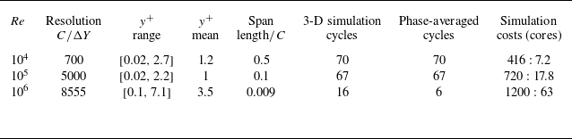
Resolution for three
 $ \textit{Re}$
values. The
 $y^+$
values are the first grid inside BDIM
 $\epsilon$
. The total cycles of 3-D simulations exclude the preceding 2-D simulations. The phase-averaging for
 $ \textit{Re}=10^6$
is conducted at the last 6 cycles to exclude the transient phases. The last column contains information of CPU-core usage and simulation length in hours per cycle.

Table 2. Long description
A table comparing simulation parameters for different Reynolds numbers. The table has six rows and eight columns. The columns are labeled Re, Resolution C/ΔY, y+ range, y+ mean, Span length/C, 3-D simulation cycles, Phase-averaged cycles, and Simulation costs (cores). The rows present data for three different Reynolds numbers: 10^4, 10^5, and 10^6. Row 1: Re 10^4, Resolution 700, y+ range [0.02, 2.7], y+ mean 1.2, Span length/C 0.5, 3-D simulation cycles 70, Phase-averaged cycles 70, Simulation costs (cores) 416 : 7.2. Row 2: Re 10^5, Resolution 5000, y+ range [0.02, 2.2], y+ mean 1, Span length/C 0.1, 3-D simulation cycles 67, Phase-averaged cycles 67, Simulation costs (cores) 720 : 17.8. Row 3: Re 10^6, Resolution 8555, y+ range [0.1, 7.1], y+ mean 3.5, Span length/C 0.009, 3-D simulation cycles 16, Phase-averaged cycles 6, Simulation costs (cores) 1200 : 63.
(a) Diagram of the foil and the streamwise velocity
 $U$
with its normal (
 $y$
) and tangential (
 $x$
) axes. (b) Flapping foil phases in time
 $t$
over a cycle period
 $T$
. For discussion, phases
 $t$
correspond to the upper side of the foil, while the lower part experiences
 $t \pm 0.5T$
.

Figure 1. Long description
A diagram of a foil and its flapping phases over a cycle period. Panel A: Diagram of the foil and the streamwise velocity with its normal and tangential axes. The foil is shown in a three-dimensional space with axes labeled X, Y, and Z. The streamwise velocity is indicated with a vector labeled u. The foil has a chord length labeled C, and a pitch pivot point at 0.25C. The span of the foil is also labeled. The normal and tangential axes are labeled y and x, respectively. Panel B: Flapping foil phases in time over a cycle period T. The phases are shown as a series of images of the foil at different positions along a timeline. The timeline is labeled with time fractions t/T, ranging from 1.0 to 0.125. The foil is shown in different positions corresponding to these time fractions, indicating the flapping motion over one cycle period.
We discuss the comparison for
 $ \textit{Re}=10^4$
,
 $10^5$
and
 $10^6$
for this study in § 3. We limit
 $ \textit{Re}$
to one million due to the high computational cost of wall-resolved large-eddy simulations, and table 2 shows that our near-wall resolutions and number of cycles had to be reduced for that case compared to the lower
 $ \textit{Re}$
. Later in § 3, we notice that the phase averaging at
 $ \textit{Re}=10^6$
for six cycles was insufficient to completely smooth out the fluctuations, and might need more resolution near the trailing-edge region. However, this limitation does not change the conclusion of the study, especially the trends with increasing
 $ \textit{Re}$
. Similarly, the lack of resolution affects only the flow downstream near the outlet boundary.
2.3. Cycle phases
In the results discussion, we will present data for 32 phases per cycle as per figure 1(b). The results will only represent the upper side of the foil experiencing phases per cycle
 $t/T$
. Later, we show the span and phase averaging results as presented in table 2 for phase-averaged cycles. Since the foil is symmetrical, the lower side experiences the same states as the upper side after a half-cycle or
 $t/T+0.5$
. In the results, the first phase starts when the foil moves upwards,
 $t/T=0.03125$
, and ends at phase
 $t/T=1$
when the foil’s pivot is at location
 $Y=0$
. The cycle restarts after
 $t/T=1$
or is equivalent to
 $t/T=0$
. The projected positions are presented in 100
 $x/C$
equispaced locations on the foil as depicted in figure 1(a).
Later in the results section, we present parameters needed to compute the boundary-layer edge velocity
 $u_e$
. We use the method of velocity reconstruction from pressure data based on Bernoulli’s equation by Griffin et al. (Reference Griffin, Fu and Moin2021) to locate the boundary-layer edges (
 $\delta _e$
), while the velocity field is not modified. It has been compared with other methods, such as by Uzun & Malik (Reference Uzun and Malik2021). This method is suitable because the velocity profiles expand and retract dynamically along the phases and locations, as explained in Zurman-Nasution et al. (Reference Zurman-Nasution, Weymouth and Ganapathisubramani2024).
3. Results
3.1. Comparison with experiments
Despite the scarcity, we found comparison studies for our flapping foil studies at
 $ \textit{Re} \geqslant 10^5$
, such as the experiment of swimming rainbow trout by Yanase & Saarenrinne (Reference Yanase and Saarenrinne2015) at body length
 $ \textit{Re}_{\textit{BL}} \approx 10^5$
, and the study of FPG effects on axisymmetric turbulent boundary layers by Warnack & Fernholz (Reference Warnack and Fernholz1998). The rainbow trout experiments recorded unsteady velocity profiles, while the FPG is a quasi-steady experiment. Despite the steadily imposed pressure gradient, the FPG experiment provides a gradual boundary-layer transition towards relaminarisation, comparable to the unsteady cases of a flapping foil and a swimming fish. By matching the boundary-layer characteristics, such as the shape factors
 $H=\delta ^*/\theta$
(ratio of displacement
 $\delta ^*=\int ^{\delta _e} ( 1 - ({u}/{u_e}) )\, {\rm d}y$
to momentum thicknesses
 $\theta =\int ^{\delta _e} ( {u}/{u_e}) ( 1 - ( {u}/{u_e}) )\, {\rm d}y$
), we recover similar velocity profiles as shown in figure 2. One sample in the current study is relatively close to the momentum thickness Reynolds numbers
 $ \textit{Re}_{\theta }$
(Warnack & Fernholz Reference Warnack and Fernholz1998), but the friction velocities
 $u_{\tau }$
are completely different. There is no information on
 $ \textit{Re}_{\theta }$
and
 $u_{\tau }$
from the experiments of swimming rainbow trout for comparison.
Velocity profile comparison of the current study (blue lines) with experiments. The current study is at
 $ \textit{Re}=10^5$
at several
 $t/T$
phases and
 $x/C$
locations. Presented experiments are from the rainbow trout experiment by Yanase & Saarenrinne (Reference Yanase and Saarenrinne2015) on convex motion (unknown
 $u_{\tau }$
and
 $ \textit{Re}_{\theta }$
), and the turbulent boundary layer at FPG by Warnack & Fernholz (Reference Warnack and Fernholz1998). Despite having different
 $u_{\tau }$
, the profiles show similar extended laminar regions.

We found that the velocity profiles in our flapping foil study exhibit similarities to the rainbow trout experiment, including a distinct extended laminar region beyond
 $y^+=11$
. Most velocity profiles in the present study show extended laminar regions. While deviations from ZPG log law are expected in non-equilibrium boundary layers, the present study examines systematically the characterisation of laminar-like velocity profiles across a wide range of Reynolds numbers. Figure 2 shows the shape factor
 $H\approx 1.7$
, considered far lower than the classical laminar profile (
 $H \geqslant 2.6$
). In fact, this phenomenon is considered in a transitional state between turbulent and laminar under the influence of accelerating flow mentioned by Schlichting & Kestin (Reference Schlichting and Kestin1979). It explains why the flapping foil’s velocity profiles are similar to Warnack & Fernholz (Reference Warnack and Fernholz1998) and Balin & Jansen (Reference Balin and Jansen2021) in their quasi-steady experiment for examining the relaminarisation cases, showing laminar-like profiles. In the case of a stationary foil at
 $ \textit{Re}=10^5$
and angle of attack lower than
 $\alpha _{\textit{eff}}=23.8^{\circ }$
, the flow would have experienced strong separation or stall-triggered turbulent flow as seen in the study of Vinuesa et al. (Reference Vinuesa, Negi, Atzori, Hanifi, Henningson and Schlatter2018). Flapping foils are known to experience dynamic stall, which delays the separation.
Patel & Head (Reference Patel and Head1968) referred to the relaminarisation phenomenon as a reverse transition, and suggested that its onset happens in the boundary layer mostly under a strong FPG, and is independent of the boundary-layer characteristics such as
 $H$
or
 $ \textit{Re}_{\theta }$
. Apart from similar
 $H$
, both
 $u_\tau$
and
 $ \textit{Re}_{\theta }$
in this study can be different, as shown in figure 2. However, the values of non-dimensionalised pressure gradient
 $\varDelta _P$
are below the threshold −0.018, indicating the influence of APG. Patel & Head (Reference Patel and Head1968) (on p. 376) show a similar example where strong pressure gradients cause a major departure from the semi-logarithmic law, not only for APGs but also for FPGs.
These comparisons provide a validation of a similar phenomenon seen in flapping foil profiles with the unsteady and quasi-steady experiments, i.e. the strong influence of pressure gradients, and the appearance of an extended laminar region. In § 3.4, we will examine the effects of pressure gradient on flapping foils, and discuss the mechanism that explains the extension of the viscous region beyond
 $y^+=11$
, as well as its relationship to relaminarisation. The next subsection discusses the effect of the pressure gradient originating from the outer part of the boundary layer.
3.2. Freestream region influence
Figure 3 shows the pressure and velocity variation at height
 $y=0.1C$
above the foil, or the freestream region, as a function of length along the foil, and phase in the motion cycle across the three Reynolds numbers.
The heat maps of (a) pressure coefficients
 $Cp$
, (b) streamwise local velocities
 $u/U_{\infty }$
, and (c) pressure gradient
 ${\textrm {d}}{p}/{\rm d}{(x/C)}$
at height
 $0.1C$
from the upper side wall of the foil at
 $ \textit{Re}=10^5$
. The horizontal axis is the projected position on the upper foil
 $x/C$
representing space, and phase
 $t/T$
on the vertical axis represents the time evolution of the flow. All are span- and phase-averaged data, with selected contour lines to compare different
 $ \textit{Re}$
. At height
 $0.1C$
, the heat map represents the freestream region. Double-headed arrows (cyan) show the deviated contour at
 $ \textit{Re}=10^4$
due to an LEV. Green arrows with numbers are given for later discussion in figure 5.

Figure 3. Long description
Three heat maps illustrate different flow characteristics at a specific height from the upper side wall of a foil. Panel A: The heat map shows pressure coefficients with the horizontal axis representing the projected position on the upper foil and the vertical axis representing phase. The color scale ranges from -3 to 3, with contour lines indicating different Reynolds numbers (Re = 10^4, 10^5, 10^6). Panel B: The heat map displays streamwise local velocities normalized by freestream velocity. The horizontal axis is the projected position on the upper foil, and the vertical axis is phase. The color scale ranges from -1.0 to 2.5, with contour lines for different Reynolds numbers. Panel C: The heat map represents the pressure gradient. The horizontal axis is the projected position on the upper foil, and the vertical axis is phase. The color scale ranges from -10 to 10, with contour lines for different Reynolds numbers. Cyan double-headed arrows indicate deviated contours due to a leading-edge vortex (LEV), and green arrows with numbers are marked for later discussion.
The pressure coefficient heat map in figure 3(a) shows that the suction region (negative
 $Cp$
values) occurs in phases
 $ 0.3 \leqslant t/T \leqslant 0.7$
and is fairly uniform from the leading to the trailing edges. Each side of the foil experiences alternately the pressure side or the suction side once each per cycle.
In figure 3(b), the local velocities
 $u/U_{\infty }$
at height
 $0.1C$
show that each foil side experiences alternating high (a peak) or low (a valley), but they are not uniform along the chord length. Each foil side can experience different velocities in one phase. For example, at phase
 $t/T\approx 0.5$
, the leading edge experiences a much higher velocity than the inflow with
 $u \gt 1.75U_{\infty }$
, while the trailing edge experiences
 $u \lt 0.5U_{\infty }$
. The velocity contours show an inclination of approximately a half-cycle (
 $0.5T$
) from the leading edge at
 $t/T \approx 0.5$
to the trailing edge
 $t/T \approx 1$
. This half-cycle inclination is due to the sinusoidal flow advection from the prescribed flapping kinematics.
We also present the pressure gradient evolution
 ${\textrm {d}}{p}/{\rm d}{(x/C)}$
in figure 3(c) at height
 $0.1C$
. Each position of
 $x/C$
alternates twice per cycle between APGs in red and FPGs in blue, with two distinct APG regions. Strong but narrow APG and FPG regions happen near the leading edge, while the trailing edge is clipped by the wake. The trend of APG and FPG is inclined similarly to the velocity, following the flow advection trend.
At height
 $0.1C$
, increasing Reynolds numbers do not show a significant difference, as shown by the majority of the contour lines of different
 $ \textit{Re}$
. There is data noise for
 $ \textit{Re}=10^6$
, especially near the trailing edge, due to the limited number of cycles for phase averaging. We can see that the variation is minimal for all
 $ \textit{Re}$
, with an exceptional deviation caused by a single LEV affecting the
 $y=0.1C$
region for
 $ \textit{Re}=10^4$
. The arrow marked ‘Pinch’ in figures 3(b) and 3(c) at
 $t/T=0.75$
and
 $x/C=0.34$
shows the contour deviation of
 $ \textit{Re}=10^4$
from other
 $ \textit{Re}$
cases, causing a ’pinched’ contour of
 $u/U_{\infty }=1.5$
. At the subsequent phase and at
 $x/C=0.45$
, the APG region for
 $ \textit{Re}=10^4$
starts ’branching’ (see figure 3
c). The upper branch with
 ${\textrm {d}}{p}/{\rm d}{(x/C)} \gt 0$
follows advection similar to that of the other higher-
 $ \textit{Re}$
cases, while the lower branch shows an elongated APG region extending downwards. This branch undergoes a shorter distance
 $\Delta x/C$
over the same interval
 $\Delta t/T$
as the upper branch, indicating a slower advection caused by an LEV. A large LEV is advected more slowly than the half-cycle advection due to its size. We discuss further in the next subsection how larger vortices tend to be advected more slowly than smaller ones.
3.3. Vortex structures
Increasing Reynolds numbers produce very distinct vortex structures generated by flapping foils, especially the LEVs. Figure 4 presents the instantaneous vortex structures at
 $t=T$
. The vorticity at
 $ \textit{Re}=10^4$
is essentially 2-D (see figure 4
a), matching the results from previous low-
 $ \textit{Re}$
studies in the optimal
 $0.15 \leqslant St \leqslant 0.45$
range (Zurman-Nasution et al. Reference Zurman-Nasution, Ganapathisubramani and Weymouth2020). A single large LEV affects the flow even at height
 $0.1C$
, as previously pointed out by double-headed cyan arrows in figures 3(b) and 3(c).
Instantaneous vortex structures are represented by (a) volume render of spanwise vorticity of
 $ \textit{Re}=10^4$
, (b) contour of 0.1 % maximum
 $\lambda _2$
of
 $ \textit{Re}=10^5$
, and (c)
 $ \textit{Re}=10^6$
. The upper foil experiences phase
 $t/T=1$
or the last cycle, while the lower foil experiences
 $t/T=0.5$
. Colours represent spanwise vorticity normalised by the chord and the freestream velocity. The LEV advection is quantified by (d) the
 $\omega _z$
-weighted streamwise velocity
 $u^*_{\textit{LEV}} = ({\int (u_x/U_{\infty })\, |\omega _z| \, {\rm d}V_{\textit{LEV}}})/({\int |\omega _z| \, {\rm d}V_{\textit{LEV}}})$
, and (e) the normalised LEV volume
 $V^*_{\textit{LEV}} = ( {1}/{C^3})\int {\rm d}V_{\textit{LEV}}$
, where
 $u_x$
is the local streamwise velocity parallel to
 $C$
. The integration domain of
 $V_{\textit{LEV}}$
is restricted to the upper side of the foil,
 $0\lt x/C\lt 1$
,
 $y\lt 0.1C$
, and
 $\lambda _2\lt 0$
for LEV centroid locations.

This 2-D flow cannot be maintained at higher
 $ \textit{Re}$
, as seen in figures 4(b,c). The flapping foil generates LEVs near the leading edge during the suction phase of each cycle, alternately on the upper or lower side. There is a single LEV at
 $ \textit{Re}=10^4$
, but the flow produces smaller, more compact vortices and in much greater quantities as
 $ \textit{Re}$
increases. These vortices are advected downstream and become unstable as the boundary layer grows, evolving into fully 3-D vortex structures from approximately
 $0.4C$
to the last half of the chord length. As expected, the flow at
 $ \textit{Re}=10^6$
is noisier and more chaotic than at lower
 $ \textit{Re}$
, especially near the trailing edge.
The normalised LEV volume or
 $V^*_{\textit{LEV}}$
in figure 4(e) represents the reduction of the LEV centroid region (
 $\lambda _2\lt 0$
) with increasing
 $ \textit{Re}$
, which is further referred to as LEV size reduction. The LEV size increases slightly during its appearance in the second half of the cycle (
 $ 0.5 \leqslant t/T \leqslant 1$
), but the ordering with respect to
 $ \textit{Re}$
remains unchanged. Each LEV circulation increases with
 $ \textit{Re}$
(data not presented for conciseness), but the normalised volume decreases substantially, indicating increased LEV compactness with an increased quantity of smaller LEVs. The LEV vorticity-weighted streamwise velocity
 $u^*_{\textit{LEV}}$
in figure 4(d) is seen to increase during the last half of the cycle following the increase in
 $ \textit{Re}$
, indicating an increase in advection speed.
3.4. The phase evolution of velocity profiles and near-wall pressure gradients
We found that the extended laminar profile at each location on the foil or the relaminarisation described in § 3.1 is promoted by the FPG, whereas APG reverses it. The green arrows on the freestream pressure gradient in figure 3(c) can be compared to the pressure gradient near the wall in figure 5(b). The freestream region outside the boundary layer acts as forcing, accelerating the flow inside the boundary layer, as shown in figure 5(a) (circled 2). This FPG acceleration causes the velocity profile to rapidly inflate the laminar-like region of the boundary layer. The whole boundary layer might not inflate, as the FPG tends to reduce the boundary-layer momentum or displacement thicknesses. This expanding laminar part of the boundary layer is also more prominent with the increase of
 $ \textit{Re}$
, with the
 $ \textit{Re}=10^6$
boundary layer tripling in size for
 $t/T=0.43{-}0.53$
. Hence the relaminarisation is stronger at higher
 $ \textit{Re}$
.
(a) Evolution of velocity profiles when exiting APG (circled 1), exiting FPG (circled 2), and inside vortex breakdown region (circled 3) at
 $x/C=0.45$
. (b) Heat maps of the near-wall pressure gradient for increasing
 $ \textit{Re}$
. Green arrows follow the direction of increasing phase
 $t/T$
, and the magenta arrow shows the trend of increasing
 $ \textit{Re}$
. Velocity profiles and wall pressure gradients
 ${\textrm {d}}{p}/{\rm d}{(x/C)}_{wall}$
are span- and phase-averaged.

Figure 5. Long description
The image contains two sets of graphs. The first set (a) consists of three line graphs showing the evolution of velocity profiles at different phases. Each graph has a horizontal axis labeled y+ (yuτ/ν) and a vertical axis labeled u+ (u/ut). The graphs are labeled 1, 2, and 3, corresponding to different regions: exiting adverse pressure gradient (APG), exiting favorable pressure gradient (FPG), and inside vortex breakdown region, respectively. The graphs include multiple lines representing different time fractions (t/T) and Reynolds numbers (Re). The second set (b) consists of three heat maps showing the near-wall pressure gradient for increasing Reynolds numbers (Re = 10^4, 10^5, 10^6). Each heat map has a horizontal axis labeled x/C and a vertical axis labeled Phase t/T. The heat maps use a color scale to represent the pressure gradient (dp/d(x/C)wall), with red indicating positive values and blue indicating negative values. Green arrows indicate the direction of increasing phase, and a magenta arrow shows the trend of increasing Reynolds number.
On the contrary, the APG reverses the expansion of the laminar region. When the flow is at the APG, the relaminarisation process is reversed as in figure 5 marked by circled 1 and also circled 3. The extended laminar regions shrink during this phase as they move away from the linear curve
 $u^+=y^+$
and closer to the log profile. However, the shrinkage order based on increasing
 $ \textit{Re}$
at circled 3 no longer follows the same trend as in circled 1. This is because the advection at circled 3 of vortex breakdown now influences the flow in addition to the APG condition.
Heat maps in figure 5(b) show that pressure gradients at the wall differ for each
 $ \textit{Re}$
. The breakdown of vortices is related to the pressure gradient distribution, as indicated by the flickering blue–red areas just after phase
 $t/T=0.5$
. The LEVs at higher
 $ \textit{Re}$
are smaller but more compact, experiencing faster advection, and thus have a shorter spatial footprint and reduced interaction with the wall. We see the same ‘branching’ APG for
 $ \textit{Re}=10^4$
as explained in § 3.2 at figure 3(c) for pressure gradient. One ends before
 $t/T=1$
, while the other transports an LEV to the next cycle. The phase interval
 $\Delta t/T$
spent by smaller vortices for higher
 $ \textit{Re}$
advected downstream is a half-cycle or less, while an LEV at
 $ \textit{Re}=10^4$
needs a
 $1.5$
times longer interval. The arrow marked by circled 3 is at the onset of LEV advection for
 $ \textit{Re}=10^4$
, while it is inside the advection region of LEV breakdown for
 $ \textit{Re}=10^5$
, and has just passed through at
 $ \textit{Re}=10^6$
. The reverse effect of relaminarisation ends faster at higher
 $ \textit{Re}$
due to faster advection.
3.5. Indication of relaminarisation and cyclic behaviour
Figure 6(a) illustrates the cyclic evolution of the normalised boundary layer edge velocity
 $u_e/U_{\infty }$
, the zero-mean fluctuation of wall-friction coefficient
 $c_{\kern-1pt f}^{\prime}$
, friction velocity
 $u_{\tau }$
, displacement thickness
 $\delta ^*$
, and shape factor
 $H$
at approximately mid position,
 $x=0.45C$
. Here,
 $c_{\kern-1pt f}^{\prime}$
is the zero-mean fluctuation of
 $c_{\kern-1pt f}=2(u_{\tau }/u_e)^2$
, where the average across phase
 $t/T$
is removed at each position
 $x/C$
. During the expansion of the laminar-like region marked by circled 2 (the same as in figures 3(b) and 5), the freestream velocity is positive and the flow is accelerating or at FPG state. Region circled 2 begins with the peak of
 $c_{\kern-1pt f}^{\prime}$
, followed by a rapid decrease by 31 % for an eighth of a cycle. Mukund et al. (Reference Mukund, Viswanath, Narasimha, Prabhu and Crouch2006) and Uzun & Malik (Reference Uzun and Malik2021) found a similar trend of decrease. This condition is accompanied by an 8.5 % increase in
 $H$
. On the contrary, the APG areas of circled 1 and circled 3 indicate an increase of
 $c_{\kern-1pt f}^{\prime}$
by double and 62 %, along with the decrease of
 $H$
by 15 % and 2 %. Friction velocity
 $u_{\tau }$
follows the same trend as
 $c_{\kern-1pt f}^{\prime}$
, with a slight delay. Displacement
 $\delta ^*$
is at its lowest value during FPG, with a sudden increase by 35 % occurring at circled 3 mostly due to the APG region and downstream vortices. However, no clear trend can be inferred during the APG at circled 1 and the FPG at circled 2 due to subtle variations. Both boundary-layer displacement
 $\delta ^*$
and momentum thickness
 $\theta$
(not shown) show a similar trend.
(a) Evolution of variables per cycle at
 $ \textit{Re}=10^5$
and position
 $x/C=0.45$
. Values are span- and phase-averaged. Green-shaded areas correspond to green arrows in figure 5. The correlation of
 $c_{\kern-1pt f}^{\prime}$
with (b)
 $H$
and (c)
 $\delta ^*$
is quantified using Pearson’s correlation coefficient
 $r$
. The moderate-to-high positive or negative correlations are defined by
 $|r| \geqslant 0.45$
, whereas the grey-shaded region denotes weak correlation.

The consistent trend of
 $H$
following the inverse variation of
 $c_{\kern-1pt f}^{\prime}$
throughout the flapping cycle indicates that both quantities respond to the same near-wall momentum redistribution. The cyclic evolutions of
 $H$
are closely related to
 $c_{\kern-1pt f}^{\prime}$
, as shown in figure 6(b) by moderate to strong inverse correlation on each position on the foil. At
 $ \textit{Re}=10^6$
and
 $x/C\gt 0.6$
, the correlation decreases due to the high signal-to-noise ratio in phase-averaging, but it does not diminish the overall trend. In contrast, the correlation between
 $c_{\kern-1pt f}^{\prime}$
and displacement thickness
 $\delta ^*$
(similarly for
 $\theta$
) in figure 6(c) is inconsistent and generally weaker at both the highest and the lowest
 $ \textit{Re}$
across nearly all positions on the foil. This difference suggests that
 $H$
is strongly associated with the inner-layer dynamics, or sensitive to profile reshaping, whereas thickness measures are more influenced by global boundary-layer growth. Even though classical equilibrium laminar–turbulent interpretations might not fully apply to flapping foil flow,
 $H$
remains a physically interpretable measure.
Cyclic behaviour of
 $c_{\kern-1pt f}^{\prime}$
at
 $x/C=0.2$
and
 $0.72$
for different
 $ \textit{Re}$
. Correlation lines are shown for Blasius (laminar) and Coles–Fernholz (turbulent). Arrows and colours (see legend) show forward in phase
 $t/T$
. Low-
 $ \textit{Re}$
cycles are closer to laminar, but the higher-
 $ \textit{Re}$
cycles intermittently switch between laminar and turbulent.

Figure 7. Long description
Two line graphs depict the cyclic behavior of skin friction coefficient at different chordwise positions. Panel A shows data for x over C equals 0.20, while Panel B shows data for x over C equals 0.72. Both graphs plot skin friction coefficient c subscript f prime on the vertical axis against Reynolds number Re subscript theta on the horizontal axis. The data points are color-coded to represent different phases within the cycle, with a color bar indicating the phase fraction t over T. The graphs include correlation lines for Blasius (laminar) and Coles-Fernholz (turbulent) models. Arrows indicate the forward progression in phase. Low Reynolds number cycles are closer to laminar behavior, while higher Reynolds number cycles intermittently switch between laminar and turbulent states.
Graphs in figure 7 demonstrate that each location
 $x/C$
exhibits a cyclic behaviour of the friction coefficient fluctuation
 $c_{\kern-1pt f}^{\prime}$
that intermittently approaches either laminar or turbulent limits. Here, the laminar correlation is presented by the Blasius line, where
 $c_{\kern-1pt f}=(0.664^2)/Re_{\theta }$
, and turbulent at ZPG by the Coles–Fernholz correlation, where
 $c_{\kern-1pt f}=2 ( ( {1}/{0.41}) \log (Re_{\theta })+4.127 ) ^{-2}$
. Increasing global
 $ \textit{Re}$
also increases
 $ \textit{Re}_{\theta }$
, shifting the cycles to the right-hand side of the graph. However, each chordwise location exhibits different cyclic behaviours. Near the upstream locations (
 $x/C=0.2$
), the
 $c_{\kern-1pt f}^{\prime}$
cycles are closely aligned with the Blasius or laminar correlation limit even for
 $ \textit{Re}=10^6$
. Moving closer to the trailing edge at
 $x/C=0.72$
, they begin to approach the turbulent correlation line, especially at higher
 $ \textit{Re}$
. Figure 7 indicates that most cycles at
 $ \textit{Re}=10^4$
stay laminar, while
 $c_{\kern-1pt f}^{\prime}$
at higher
 $ \textit{Re}$
indicates a cyclic behaviour between laminar and turbulent.
3.6. Failure of the standard relaminarisation criteria
Several criteria for relaminarisation or flow reversion are summarised by Narasimha & Sreenivasan (Reference Narasimha and Sreenivasan1979) from various studies based on the velocity profile deviations from the standard log law in steady or quasi-steady cases. These criteria are systematically proven to be inconsistent when applied as a diagnostic benchmark for flapping foil flows. Criteria for relaminarisation occur when
 $K=({\nu }/{\rho u_e^2})({{\rm d}u_e}/{{\rm d}x}) \gtrsim 3.5 \times 10^{-6}$
,
 $\varDelta _p =-( {\nu }/{\rho u_{\tau }^3}) \left .( {{\rm d}p}/{{\rm d}x})\right \vert _{wall} \gtrsim 0.025$
and
 $\varDelta _{\tau } =\left .( {\nu }/{u_{\tau }^3})( {{\rm d} \tau }/{{\rm d}y})\right \vert _{wall} \lesssim 0.009$
.
(a) Decelerating and (b) accelerating flow (relaminarisation) at phase
 $t/T=0.75$
at
 $ \textit{Re}=10^5$
are observed for the deviation from the standard log law. The variable nominals are indicated in the table.

Figure 8 illustrates the velocity profile evolution on sequential chordwise positions in one phase, and the alignment with the standard log law. Figure 8(a) shows a decelerating flow where we observe a deviation of velocity profiles from the log law at positions
 $0.17\leqslant x/C \leqslant 0.18$
, while
 $0.19\leqslant x/C \leqslant 0.21$
reverts to the log law. However,
 $K$
falls below its criterion starting at
 $x/C \geqslant 0.18$
, earlier than the change observed in velocity profiles. The
 $\varDelta _{\tau }$
values fall below zero, while
 $\varDelta _p$
increases, indicating APG, but neither aligns with the criteria. Figure 8(b) shows an accelerating flow, where relaminarisation and deviations from the log law are expected at
 $x/C \geqslant 0.42$
. Also,
 $K$
exceeds its criterion later at
 $x/C \geqslant 0.43$
,
 $\varDelta _p$
exceeds the criterion only within
 $0.44\leqslant x/C \leqslant 0.45$
, and
 $\varDelta _{\tau }$
remains below the criterion throughout.
The inconsistencies with flow-reversion limits mentioned in the literature might be attributed to the reliance on a constant pressure gradient and the absence of phase-history effects. While their applicability to strongly unsteady boundary layers in flapping foils is expected to be limited, their predictive capability is systematically assessed as a baseline for comparison. Subtracting the influence from upstream flow or previous phases requires a more controlled condition. Any apparent agreement with the log law should be interpreted as a transient behaviour rather than a sustained equilibrium state. The obvious indications of the log-law departure for the flapping foil observed in this study occur when the friction coefficient
 $c_{\kern-1pt f}^{\prime}$
decreases while the shape factor increases above the transitional turbulence
 $H \gtrsim 1.8$
. Determining precise limits remains a topic for future work.
3.7. Wall friction fluctuation and the Clauser parameter
The previous subsections provide a clear indication that both the shrinkage and contraction of the laminar-like regions are directly related to the wall friction coefficient fluctuation (
 $c_{\kern-1pt f}^{\prime}$
). Therefore, it is essential to examine how it behaves with increasing
 $ \textit{Re}$
.
Heat maps of (a) the wall friction coefficient
 $c_{\kern-1pt f}$
and (b) friction velocities
 $u_{\tau }$
of
 $ \textit{Re}=10^5$
along the streamwise location and phase. The zero-mean RMS (or standard deviation) of (c)
 $c_{\kern-1pt f}$
and (d)
 $u_{\tau }$
with increasing
 $ \textit{Re}$
represents the fluctuation along the phases. Here,
 $c_{\kern-1pt f}$
and
 $u_{\tau }$
are span- and phase-averaged.

Figure 9. Long description
The image contains four panels: two heat maps and two line graphs. Panel A shows a heat map of the wall friction coefficient along the streamwise location (x/C) and phase (t/T). The color scale on the right indicates the values of the wall friction coefficient, ranging from 0 to 0.02. Panel B displays a heat map of friction velocities along the same axes, with a color scale ranging from 0 to 0.12. Panel C presents a line graph of the zero-mean RMS (standard deviation) of the wall friction coefficient for different Reynolds numbers (Re = 10^4, Re = 10^5, Re = 10^6) along the streamwise location (x/C). The graph shows how the fluctuation along the phases varies with increasing Reynolds numbers. Panel D illustrates a line graph of the zero-mean RMS of friction velocities for the same Reynolds numbers along the streamwise location (x/C). The graphs indicate trends and patterns in the data, showing how the Reynolds number affects the fluctuations in the boundary layer.
Figures 9(a,b) are heat maps of the friction coefficient
 $c_{\kern-1pt f}$
and the friction velocity
 $u_{\tau }$
variables for
 $ \textit{Re}=10^5$
, where the trace of vortex breakdown is seen in the phase region
 $0.5 \lesssim t/T \lesssim 1$
. Similar patterns of vortex advection are observed at other Reynolds numbers (refer to Appendix A), although each
 $ \textit{Re}$
exhibits distinct fluctuation distributions. The lowest values, depicted in the lightest colour, are primarily observed in the region of LEV breakdown and its advection towards the trailing edge. Lower
 $c_{\kern-1pt f}$
values are associated with turbulence.
We obtain the cyclic fluctuation across a cycle
 $T$
for
 $c_{\kern-1pt f}$
and
 $u_{\tau }$
by zeroing the mean values at each
 $x/C$
from heat maps in figures 9(a,b). To compare fluctuations across different
 $ \textit{Re}$
, we compute the standard deviation of
 $c_{\kern-1pt f}$
and
 $u_{\tau }$
, or zero-mean root mean square (RMS) in figures 9(c,d). The
 $c_{\kern-1pt f}$
RMS decreases with the increase of
 $ \textit{Re}$
, likely due to the decrease of the
 $u_{\tau }$
RMS, even though the velocities at the freestream or boundary-layer edge are similar for all
 $ \textit{Re}$
. Increased
 $ \textit{Re}$
generates multiple, smaller, more compact vortices, causing early and rapid vortex breakdown. This reduces the coherence and phase-localised vortex–wall interaction, leading to a smaller peak-to-trough cyclic modulation of wall shear, i.e. lower
 $c_{\kern-1pt f}$
RMS and
 $u_{\tau }$
RMS. In Appendix A,
 $ \textit{Re}=10^4$
exhibits the highest contrast between the LEV area and its surroundings at the leading edge, explaining this high fluctuation across the cycle phase or higher RMS. The flow remains turbulent near the trailing edge at
 $ \textit{Re}=10^6$
, mainly because the fluctuation of
 $u_{\tau }$
increases, or the turbulence level is stronger. The moderation of
 $c_{\kern-1pt f}$
RMS towards the trailing edge, unlike
 $u_{\tau }$
, is caused by the increase of the denominator
 $u_e$
values and
 $u_e$
RMS.
Clauser’s pressure gradients parameter
 $\beta _{CL}$
normalised by displacement thickness
 $\delta ^*$
and wall shear stress
 $\tau _w$
(Clauser Reference Clauser1954). Greys have no data, and only the first front halves of the chord locations are provided for
 $ \textit{Re}=10^6$
due to a high signal-to-noise ratio.

Figure 10 illustrates the normalised pressure gradient parameter of Clauser (Reference Clauser1954) as
 $\beta _{RC}=({\delta ^*}/{\tau _w})( {{\rm d}p}/{{\rm d}x})$
. Identical values of
 $\beta _{RC}$
indicate the same ratio of pressure gradient over wall shear stress, and a similar shape factor under certain conditions. Positive values indicate APG, and negative values indicate FPG. The
 $\beta _{RC}$
are distributed similarly to the near-wall pressure gradient in figure 5(b), with two significant APG regions. However, we can more clearly observe the regions where LEVs are first generated (marked ‘LEV’), followed by their downstream advection traces in later phases. With increasing
 $ \textit{Re}$
, the LEV influence is pushed closer to the leading edge, a sign of early LEV generation. At
 $ \textit{Re}=10^6$
, the LEV region narrows significantly and is much closer to the foil’s leading edge at
 $t/T \approx 0.5$
. The LEV breakdown is also advected downstream, along with the second APG region in the opposite
 $\beta _{RC}$
sign, as if it were disconnected from the region where the LEV was initially generated. It might explain why regions of downstream advection at
 $ \textit{Re}=10^6$
are not affected by the large LEV region nor promoted into fully 3-D turbulence. It also explains why
 $c_{\kern-1pt f}$
and
 $u_{\tau }$
RMS in figure 9 are smaller with increasing
 $ \textit{Re}$
. The early and narrow LEV-generated region is somehow beneficial for stabilising the LEV breakdown at higher
 $ \textit{Re}$
.
In conclusion, the FPG that promotes the expansion of the laminar-like region is not affected by the flow fluctuations caused by the breakdown of LEVs. As a result, higher
 $ \textit{Re}$
may lead to more stable or undisturbed relaminarisation. It would be interesting to investigate in the future whether this phenomenon continues to occur at even higher
 $ \textit{Re}$
.
4. Conclusion
We study the flow across three increasing Reynolds numbers,
 $ \textit{Re}=10^4$
,
 $10^5$
and
 $10^6$
, at the optimum propulsive range of flapping foil
 $ \textit{St}=0.3$
. We show that despite the similarity of freestream being given as forcing variables, different Reynolds number cases show unique trends for the variables inside the boundary layer. The freestream pressure (
 $Cp$
) and velocity (
 $u_{10C}/U_{\infty }$
) variables show similarities to the prescribed kinematics that are dominant in the region far from the boundary layer. We notice that the
 $Cp$
trend is almost constant throughout the foil position
 $x/C$
, but changes with phases following the heave kinematics. Meanwhile,
 $u_{10C}/U_{\infty }$
resembles the trend of pitch kinematics where each
 $x/C$
varies in the vertical position
 $Y$
from the leading edge to the trailing edge per phase. Both velocity and pressure gradient at the freestream exhibit the half-cycle advection trend as the prescribed sinusoidal kinematics.
The near-wall dynamics is governed by the LEV formation and breakdown. During the first half-cycle, before vortex breakdown, the wall pressure gradient follows the freestream pressure gradient. It indicates the strong influence of flapping kinematics on the flow. Under strong FPGs, the flow exhibits relaminarisation with a growing laminar-like region, consistent with Warnack & Fernholz (Reference Warnack and Fernholz1998). The second half of the flapping foil cycle is strongly influenced by LEV breakdown, which modifies the downstream boundary-layer development in subsequent phases. As the Reynolds number increases, the flapping foil generates more LEVs of a much smaller size and greater compactness, with reduced normalised volume but increased strength. They advect more rapidly, as indicated by increasing vorticity-weighted streamwise velocity, resulting in shorter vortex–wall interaction times.
Although higher
 $ \textit{Re}$
generally promotes turbulence and separation, the phase-to-phase fluctuation of the friction coefficient (
 $c_{\kern-1pt f}$
RMS) decreases with increasing
 $ \textit{Re}$
. This reflects reduced cyclic wall-shear modulation. The trend is associated with the observed confinement of the LEV-generation region towards the leading edge, which extends the downstream breakdown region and promotes earlier vortex breakdown. The increase in LEV compactness, faster advection, the confinement of the formation region, and the reduced wall-shear cyclic fluctuations lead to more persistent laminar-like behaviour at
 $ \textit{Re}=10^6$
.
Classical relaminarisation indicators under FPG proposed by Narasimha & Sreenivasan (Reference Narasimha and Sreenivasan1979) do not consistently capture the present flapping foil flows. Instead, a decrease in the cyclic fluctuation of the friction coefficient
 $c_{\kern-1pt f}^{\prime}$
and an increase in the shape factor
 $H$
during the acceleration of outer flow (
 ${\rm d}u_e/{\rm d}(x/C)\gt 0$
) provide more consistent diagnostic trends. However, defining a single global scaling for relaminarisation across phases remains challenging due to upstream conditions, phase history and LEV breakdown. Similar scaling difficulties in non-equilibrium boundary layers have been discussed by Marusic et al. (Reference Marusic, McKeon, Monkewitz, Nagib, Smits and Sreenivasan2010), and are inherent to flapping foil flows.
The reduced phase-to-phase fluctuations of
 $c_{\kern-1pt f}$
at increasing
 $ \textit{Re}$
indicate a reduction of near-wall unsteadiness, as laminar-like behaviours persist. Resolving the flow at
 $ \textit{Re}\gt 10^6$
would require substantially higher computational resources to determine whether turbulence eventually dominates over kinematic forcing. Fukagata et al. (Reference Fukagata, Iwamoto and Hasegawa2023) show drag reduction of up to 40 % due to persistent streamwise relaminarisation even at
 $ \textit{Re}_{\tau }=10^5$
in the downstream travelling wave experiment. This implies that kinematics may remain dominant in propulsive flapping foil flows, even beyond
 $ \textit{Re}=10^6$
. Such behaviour may be of interest for drag and noise reduction studies. Moreover, the persistent laminar-like behaviours facilitate numerical simulations at high
 $ \textit{Re}$
, reducing near-wall resolutions compared to stationary foil simulations at stall. Extending the present analysis to non-propulsive flapping states (e.g.
 $ \textit{St}\gt 0.5$
), where stronger instabilities and more chaotic wakes are expected, remains an important direction for future work but lies beyond the scope of the present study.
Acknowledgements
The authors would like to thank the Defence Science and Technology Laboratory UK for the earlier funding, and the IRIDIS High-Performance Computing Facility with its associated support services at the University of Southampton. They would also like to thank Professor U. Piomelli and Dr T. Nishino for informal email discussions and valuable feedback.
Declaration of interests
The authors report no conflict of interest.
Data availability statement
Data published in this article are available from the University of Southampton repository at https://doi.org/10.5258/SOTON/D3974.
Appendix A
Nominal values of wall friction coefficient
 $c_{\kern-1pt f}$
and the friction velocity
 $u_{\tau }$
for different
 $ \textit{Re}$
are shown in figure 11.
Nominal values of friction coefficient
 $c_{\kern-1pt f}$
and friction velocities
 $u_{\tau }$
of increasing Reynolds number presented on heat maps along the phases
 $t/T$
and positions on foil
 $x/C$
. Grey cells show no values. The nominal values are decreasing with
 $ \textit{Re}$
, creating a more uniform map across the phase and location, thus decreasing the fluctuation generally.

Figure 11. Long description
The image contains six heat maps arranged in a 2x3 grid. Each heat map represents data for different Reynolds numbers (10^4, 10^5, and 10^6). The top row shows the friction coefficient (Cf) and the bottom row shows the friction velocities (u_t). The x-axis for all maps is labeled x/C, ranging from 0.1 to 0.9. The y-axis is labeled Phase t/T, ranging from 0.12 to 1.00. The color scale for the top row ranges from 0 to 0.020, and for the bottom row, it ranges from 0 to 0.12. Grey cells indicate no values. The nominal values decrease with increasing Reynolds number, creating a more uniform map across the phase and location, thus decreasing the fluctuation generally.
The grid convergence study at
 $ \textit{Re}=10^4$
is presented by: (a) the
 $L_2$
norm
 $\sqrt {( {1}/{N}) \sum \nolimits _{i=1}^{N} (\sigma ^{h_{\textit{finest}}}(i)-\sigma ^h(i))^2}$
, where
 $\sigma (i)$
represents the zero-mean RMS of
 $u_{\tau }$
at the
 $i=x/C$
location, for
 $N=100$
equispaced points along the chord
 $C$
, and resolution
 $h$
; (b) the mean thrust coefficient
 $C_T$
and relative errors
 $(C_T - C_{T_{\textit{finest}}})/ C_{T_{\textit{finest}}}$
. The
 $u_{\tau }$
RMS at
 $C/\Delta Y=700$
corresponds to the same values presented in figure 9(d). The table summarises the grid resolutions
 $C/\Delta Y$
with the mean and a range of
 $y^+$
values.

Appendix B
The results in figure 12(a) present a grid-convergence study of the zero-mean RMS of
 $u_{\tau }$
, a near-wall cyclic-fluctuating quantity, exhibiting a first-order trend and decreasing monotonically with the grid refinement. The same grid-scaling strategy approximately translates to higher Reynolds number cases, with increasing
 $y^+$
in proportion to
 $u_{\tau }$
. The mean and range of the near-wall resolution
 $y^+$
remain within
 $y^+ \leqslant 7$
, and the
 $C_T$
relative errors are within 18 % in figure 12(b) for the coarsest grid. Presenting relative errors is conservative due to the near-zero values of
 $C_T$
, even though the absolute differences are small. A full convergence study at higher Reynolds numbers is computationally prohibitive, yet the trend consistency supports the robustness of the numerical set-up.
Appendix C
Figure 13 shows that both 2-D and 3-D simulations exhibit a dominant peak and the second harmonic of flapping frequency, confirming that the primary flapping-driven unsteady mechanism is preserved in both cases. The 3-D simulation displays noticeably higher broadband energy across intermediate and high frequencies compared to the 2-D simulation. This indicates the presence of additional 3-D flow structures and spanwise instabilities that redistribute energy towards smaller scales. The same conclusion is valid for
 $ \textit{Re}=10^4$
and
 $ \textit{Re}=10^6$
.
The fast Fourier transform (FFT) spectra of (a) lift (
 $C_L$
) and (b) thrust (
 $C_T$
) coefficients from 2-D and 3-D simulations at
 $ \textit{Re}=10^5$
and
 $ \textit{St}=0.3$
, representing pressure and viscous forces.

Figure 13. Long description
Two line graphs compare the FFT spectra of lift and thrust coefficients from 2-D and 3-D simulations. Panel A: The line graph shows the FFT spectrum of the lift coefficient. The x-axis represents the frequency ratio (fC/U∞) ranging from 10^-1 to 10^4, and the y-axis represents the amplitude ranging from 10^-6 to 10^0. The graph includes two data series: one for 2-D simulations in blue and one for 3-D simulations in orange. The 3-D simulation data shows higher amplitude peaks compared to the 2-D simulation data, particularly around the frequency ratio of 10^0. Panel B: The line graph shows the FFT spectrum of the thrust coefficient. The x-axis represents the frequency ratio (fC/U∞) ranging from 10^-1 to 10^4, and the y-axis represents the amplitude ranging from 10^-7 to 10^-1. Similar to Panel A, the graph includes two data series: one for 2-D simulations in blue and one for 3-D simulations in orange. The 3-D simulation data again shows higher amplitude peaks compared to the 2-D simulation data, particularly around the frequency ratio of 10^0.
The fast Fourier transform shows that the fundamental harmonic is unchanged between the 2-D and 3-D cases, indicating that the global lift and thrust remain kinematically governed, while the enhanced broadband content in the 3-D case reflects additional vortex deformation and breakdown. Thus 3-D effects introduce small-scale unsteadiness without altering the primary flapping-frequency response, consistent with spanwise LEV instability at this Reynolds number.


 St=0.3
 CT=−FX/(0.5ρSpU∞2)
 CPow=P/(0.5ρSpU∞3)
 η=CT¯/CPow¯
 FX
 Sp
 P
 ρ
 CT
 Re
 y+
 ϵ
 Re=106

 U
 y
 x
 t
 T
 t
 t±0.5T

 Re=105
 t/T
 x/C
 uτ
 Reθ
 uτ

 Cp
 u/U∞
 dp/d(x/C)
 0.1C
 Re=105
 x/C
 t/T
 Re
 0.1C
 Re=104

 Re=104
 λ2
 Re=105
 Re=106
 t/T=1
 t/T=0.5
 ωz
 uLEV∗=(∫(ux/U∞)|ωz|dVLEV)/(∫|ωz|dVLEV)
 VLEV∗=(1/C3)∫dVLEV
 ux
 C
 VLEV
 0
 y<0.1C
 λ2<0

 x/C=0.45
 Re
 t/T
 Re
 dp/d(x/C)wall

 Re=105
 x/C=0.45
 cf′
 H
 δ∗
 r
 |r|⩾0.45

 cf′
 x/C=0.2
 0.72
 Re
 t/T
 Re
 Re

 t/T=0.75
 Re=105

 cf
 uτ
 Re=105
 cf
 uτ
 Re
 cf
 uτ

 βCL
 δ∗
 τw
 Re=106

 cf
 uτ
 t/T
 x/C
 Re

 Re=104
 L2
 (1/N)∑i=1N(σhfinest(i)−σh(i))2
 σ(i)
 uτ
 i=x/C
 N=100
 C
 h
 CT
 (CT−CTfinest)/CTfinest
 uτ
 C/ΔY=700
 C/ΔY
 y+

 CL
 CT
 Re=105
 St=0.3

 Open access

